Quantification of the influence of anthropogenic and natural factors on the record-high temperatures in 2023 and 2024

The unexpectedly high global mean surface temperature (GMST) anomalies in 2023 and 2024 greatly exceeded the temperatures observed in the years directly prior. In this paper, we use a multiple linear regression energy balance model to quantify the contributions of several natural and anthropogenic factors to the GMST, including the large reduction of sulfur emissions from the shipping sector since 2020. The model is trained on 170 years of historical climate data, and allows for the attribution of warming to various natural and anthropogenic factors. The influence of anthropogenic activity on the GMST is quantified using a 160,000 member ensemble that considers the uncertainty in the magnitude of aerosol radiative forcing and the strength of climate feedbacks. We find that in response to a rise in global radiative forcing of either 0.1 or 0.15 W m⁻² due to the reduction of sulfur emissions from international shipping, the associated rise in GMST by the end of 2024 is either 0.028 °C [0.025 to 0.031 °C, 5 %–95 % range] or 0.043 °C [0.038 to 0.046 °C], respectively. We also show that approximately 0.092 °C of the rise in annual mean GMST from 2022 to 2023 can be attributed to a shift from La Niña to El Niño conditions, which is approximately a third of the observed 0.3 °C rise in GMST between these two years. Additional increases in the annual mean GMST in 2023 and 2024 (both relative to 2022) of 0.075 °C [0.036 to 0.096 °C] and 0.053 °C [0.019 to 0.074 °C] are attributed, respectively, to a strong positive Indian Ocean Dipole (IOD) event that began in 2023. Our study is the first to suggest a significant contribution from the IOD to the anomalously high values of GMST observed in 2023 and 2024. Anomalously high Sea Surface Temperatures (SSTs) in the North Atlantic region led to a rise in GMST of 0.070 °C [0.054 to 0.094 °C] and 0.069 °C [0.055 to 0.091 °C] in 2023 and 2024 relative to 2022, respectively. This contribution is almost 90 % lower when the short-term variability component of North Atlantic SSTs is removed, resulting in lower estimates of the GMST anomaly in 2023 and 2024 than observed. These results suggest that short-term variability in the North Atlantic SSTs may have played a significant role in influencing the GMST anomalies in both 2023 and 2024; however, it is unclear whether this variability is internally or externally forced. Increased incoming solar radiation due to the 11-year solar cycle led to an additional rise in GMST of 0.025 °C [−0.009 to 0.051 °C] and 0.029 °C [−0.008 to 0.056 °C] in 2023 and 2024 relative to 2022, respectively. While the 2023 and 2024 GMST anomalies can be reconstructed fairly well from a combination of natural and anthropogenic factors, uncertainties remain in the reconstruction, driven primarily by the imprecise knowledge of the radiative forcing of aerosols, and the strength of climate feedbacks.

1 Introduction

The global mean surface temperature (GMST) anomaly measured in 2023 and 2024 greatly exceeded expectations (Schmidt, 2024; Tollefson, 2025) and raised questions about the underlying cause. Several natural and anthropogenic factors, such as the onset of El Niño after a rare triple-dip La Niña event (Raghuraman et al., 2024; Terhaar et al., 2025; Blanchard-Wrigglesworth et al., 2025), a record-low planetary albedo (Goessling et al., 2025; Tselioudis et al., 2025), the eruption of the Hunga volcano (Millán et al., 2022; Vömel et al., 2022; Zhang et al., 2022; Zhu et al., 2022; Asher et al., 2023; Evan et al., 2023; Jenkins et al., 2023; Schoeberl et al., 2023, 2024; Randel et al., 2024; Gupta et al., 2025; Stenchikov et al., 2025), or the reduction of sulfur emissions from international shipping (Gettelman et al., 2024; Jordan and Henry, 2024; Quaglia and Visioni, 2024; Watson-Parris et al., 2025; Yoshioka et al., 2024; Yuan et al., 2024) are among the proposed causes of the unusually high GMST observed in 2023 and 2024.

Tropospheric sulfate aerosols, which originate from anthropogenic emissions, exhibit a considerable cooling effect on GMST (Twomey, 1974; Albrecht, 1989; Bellouin et al., 2020; Forster et al., 2021) and offset a fraction of the Greenhouse Gas (GHG) induced global warming. Efforts to improve air quality have resulted in a gradual reduction of sulfur emissions since the 1980s (Smith and Bond, 2014; Quaas et al., 2022). A new effort to improve air quality is the regulation on the sulfur content of fossil fuel used in international shipping, which began in January 2020 under the auspices of the International Maritime Organization (IMO). The IMO regulation limits the allowed sulfur content of marine fuels to 0.5 % outside of Emission Control Areas, which is much lower than the previous value of 3.5 % (IMO, 2019). Here and throughout, we refer to this regulation as IMO2020. Sulfate aerosols are major contributors to the overall Effective Radiative Forcing (ERF) from tropospheric aerosols (ERF_AER), both through the aerosol direct (ERF_ARI) and indirect (ERF_ACI) effects (Albrecht, 1989; Twomey, 1974; Szopa et al., 2021; Forster et al., 2021). Several recent studies have quantified how IMO2020 affects ERF_AER and GMST, using various observational and modelling products (Diamond, 2023; Gettelman et al., 2024; Quaglia and Visioni, 2024; Jordan and Henry, 2024; Skeie et al., 2024; Watson-Parris et al., 2025; Yoshioka et al., 2024; Yuan et al., 2024; Hansen et al., 2025). Most of these recent studies estimated the increase in ERF_AER due to IMO2020 to be in the range of 0.06 to 0.2 W m⁻². Table A1 of Jordan and Henry (2024) provides an overview of recent estimates on the impact of the IMO2020 regulations on ERF_AER.

In this paper, we quantify the impact on GMST of several natural and anthropogenic factors, including the IMO2020 regulations, using a multiple linear regression (MLR) energy balance model (EBM), the Empirical Model of Global Climate, EM–GC (Canty et al., 2013; Mascioli et al., 2012; Hope et al., 2017; McBride et al., 2021; Farago et al., 2025b). The model is trained on 170 years of historical climate data from various measurements and provides an estimate of Effective Climate Sensitivity (EffCS) of 2.63 °C [1.77 to 3.55 °C, 5 %–95 % range], which is consistent with recent literature values of EffCS described in Farago et al. (2025b). A major advantage of EM–GC is the inclusion of internal variability in simulations, a feature not present in other EBM-based analyses of the impacts of IMO2020 on GMST (Watson-Parris et al., 2025). Consequently, EM–GC has the ability to quantify the impact of various natural (such as El Niño-Southern Oscillation) and anthropogenic factors (i.e., IMO2020) on the recent GMST anomaly in a computationally efficient manner. For this paper, EM–GC was modified to include an updated two-layer ocean module that follows similar core equations as the simplified climate model (SCM) emulators used by the authors of the Sixth Assessment Report of the Intergovernmental Panel on Climate Change (IPCC AR6, Sect. 7.SM.2 of Smith et al., 2021b). A unique feature of our analysis is the quantitative evaluation of the contribution of the Indian Ocean Dipole to the GMST, a natural factor that is absent in other analyses of the GMST anomaly in 2023 and 2024.

2 Data and Methods

2.1 Empirical Model of Global Climate

In this section, we provide a brief overview of the EM–GC model, and the datasets used in this study. A more detailed description of EM–GC can be found in Farago et al. (2025b) and McBride et al. (2021). For this paper, the energy balance component of the model was updated to the two-layer EBM formulation proposed by Held et al. (2010). We briefly summarize this update in Sect. 2.1.1, and provide a more detailed description, including the calibration of the energy balance component of the model in Appendix A.

EM–GC uses an MLR analysis of the historical climate record (Lean and Rind, 2008, 2009; Foster and Rahmstorf, 2011; Zhou and Tung, 2013; Canty et al., 2013; Chylek et al., 2014) between 1850 and 2019 to compute the C₀−C₆ regression coefficients in Eq. (1), in a manner that the cost function in Eq. (2) is minimized. We refer to this process as the training of the model. The model uses a monthly time grid, with i being the indicator of a given month.

$$\begin{array}{}\text{(1)}& {\displaystyle }\begin{array}{rl}\mathrm{\Delta }{T}_{\mathrm{MDL},i}& =\mathrm{\Delta }{T}_{\mathrm{ANTH},i}+C_{\mathrm{0}}+C_{\mathrm{1}}\times {\text{SAOD}}_{i-\mathrm{6}}\\ & +C_{\mathrm{2}}\times {\text{TSI}}_{i-\mathrm{1}}+C_{\mathrm{3}}\times {\text{ENSO}}_{i-\mathrm{2}}\\ & +C_{\mathrm{4}}\times {\text{AMV}}_i+C_{\mathrm{5}}\times {\text{PDO}}_i+C_{\mathrm{6}}\times {\text{IOD}}_i\end{array}\text{(2)}& {\displaystyle }\text{Cost function}=\sum _{i=\mathrm{1}}^{N_{\mathrm{MONTHS}}}{\displaystyle \frac{\mathrm{1}}{{\mathit{\sigma }}_{\mathrm{OBS},i}^{\mathrm{2}}}}(\mathrm{\Delta }{T}_{\mathrm{OBS},i}-\mathrm{\Delta }{T}_{\mathrm{MDL},i}{)}^{\mathrm{2}}\end{array}$$

In Eq. (1), ΔT_ANTH corresponds to the change in GMST due to anthropogenic activity. This value is computed by the EBM component of our model, as described in Sect. 2.1.1 and Appendix A, from the magnitude of time-invariant climate feedback, the ERF of the climate due to GHGs, tropospheric aerosols and land-use change, as well as the export of heat to oceans. The model first computes the time series of ΔT_ANTH, after which the C₀–C₆ coefficients are quantified. ΔT_MDL and ΔT_OBS in Eqs. (1) and (2) correspond to the modelled, and observed GMST anomaly, respectively. The impact on GMST of major volcanic eruptions and variations in the intensity of solar radiation due to the 11-year solar cycle are quantified using Stratospheric Aerosol Optical Depth (SAOD) and Total Solar Irradiance (TSI), respectively. Other natural factors included in Eq. (1) are the El Niño-Southern Oscillation (ENSO), Atlantic Multidecadal Variability (AMV), Pacific Decadal Oscillation (PDO) and Indian Ocean Dipole (IOD). The SAOD, TSI and ENSO indices are lagged by 6, 1 and 2 months, respectively, following the correlation analysis described by McBride et al. (2021). The IOD term is not lagged, since the GMST anomaly found from a regression that removes the contribution of all other natural and anthropogenic factors exhibits strongest correlation with the IOD index at zero lag time (Fig. S1 in the Supplement). While we refer to AMV being a natural factor, the AMV is believed to be the result of a combination of internally and externally forced processes (Ting et al., 2009; Zhang et al., 2019b; Deser and Phillips, 2021). This important detail is addressed further in Sect. 2.2.5. The term σ_OBS,i in Eq. (2) represents the uncertainty in the observations of GMST. The use of σ_OBS,i in Eq. (2) ensures that past temperature observations that correspond to higher observational uncertainty act as weaker constraints than more recent observations.

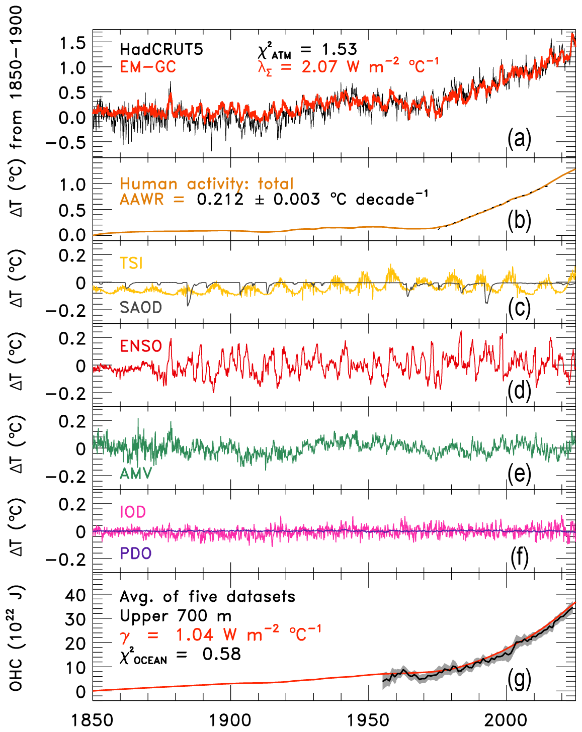
Figure 1 Single fit to the observed GMST and its decomposition to anthropogenic and natural contributions. (a) Observed (black) and modelled (red) GMST anomaly, relative to an 1850–1900 baseline. This panel also displays the values of λ_Σ and ${\mathit{\chi }}_{\mathrm{ATM}}^{\mathrm{2}}$ of this fit. (b) Contribution of anthropogenic activity (ΔT_ANTH, orange) to the modelled GMST. The value of AAWR and the corresponding 2σ uncertainty of the linear fit is also shown. This uncertainty only considers the goodness of fit between the linear fit and ΔT_ANTH, and does not account for the uncertainty in climate feedback or ERF_AER. The uncertainty in climate feedback or ERF_AER is accounted for using an ensemble method (Sect. 2.1.2). (c) Contribution of SAOD (gray) and TSI (gold) to ΔT_MDL. (d) Contribution of ENSO (red) to ΔT_MDL. (e) Contribution of AMV (green) to ΔT_MDL. (f) Contribution of IOD (pink) and PDO (purple) to ΔT_MDL. (g) Observed OHC in the upper 700 m of global oceans, based on an average of five OHC datasets (black), and modelled OHC (red). This panel also displays the values of γ and ${\mathit{\chi }}_{\mathrm{OCEAN}}^{\mathrm{2}}$. The single ensemble member shown in this figure is obtained from an EM–GC simulation trained between 1850 and 2019, for the IPCC AR6 best estimate trajectory of ERF_AER that exhibits a value of −1.1 W m⁻² in 2019, relative to 1750 (IPCC, 2021b; Smith et al., 2021a).

To illustrate the separation of ΔT_MDL to its anthropogenic and natural components that is described by Eq. (1), we show a single decomposition in Fig. 1. Panel a shows the modelled fit (ΔT_MDL, red line) to the observed GMST record obtained from version 5 of the Hadley Centre Climatic Research Unit (HadCRUT5; Morice et al., 2021, black), over 1850 to 2024. Panels (b)–(f) show the modelled contributions to the GMST from anthropogenic activity (ΔT_ANTH in Eq. (1), Fig. 1b) and natural variability (Fig. 1c–f) for this single fit. Following McBride et al. (2021), we use the slope of the linear fit to ΔT_ANTH (orange line in Fig. 1b) between 1975 and 2014 as the quantity describing the rate of rise in GMST due to anthropogenic activity, and term this metric Attributable Anthropogenic Warming Rate (AAWR). The value of AAWR for the single fit shown by Fig. 1 is given on Fig. 1b. Figure 1g shows the modelled Ocean Heat Content (OHC) in the upper 700 m of the global oceans (red), overlaid with the time series of observed OHC. The observed OHC record (black) and the corresponding uncertainty time series (grey shading in Fig. 1g) are a composite of five observational OHC datasets, described in Sect. 2.2.6. In Fig. 1g, we also display the value of the heat transfer parameter (γ, Geoffroy et al., 2013b) between the two layers of the EBM component of the model, which we describe in detail in Appendix A. The single fit shown in Fig. 1 corresponds to a given level of time-invariant climate feedback (λ_Σ, panel a) and a single time series of ERF_AER. The specific time series that is used as the input for the creation of Fig. 1 is the best estimate for the temporal evolution of ERF_AER provided by Annex III of the IPCC AR6 report (IPCC, 2021b; Smith et al., 2021a), also shown by the solid black line in Fig. S2 of Farago et al. (2025b). The parameter λ_Σ is the sum of all feedbacks (water vapor, lapse rate, clouds, etc.), except for the Planck-feedback (Farago et al., 2025b); we describe the mathematical relation of this quantity to the feedback parameter commonly used in two-layer EBMs in Appendix A.

To account for the uncertainty in the magnitude of climate feedbacks and aerosol cooling, the model performs the decomposition illustrated by Fig. 1 for a total of 160 000 ensemble members, as described in Sect. 2.1.2, where ensemble members differ in the strength of time-invariant climate feedback (λ_Σ) and the time series of ERF_AER. Each ensemble member is constrained by the model's ability to reproduce observed GMST and OHC using three reduced chi-square metrics as described in Sect. 2.1.2. The values of two of these reduced chi-square indicators (${\mathit{\chi }}_{\mathrm{ATM}}^{\mathrm{2}}$ and ${\mathit{\chi }}_{\mathrm{OCEAN}}^{\mathrm{2}}$) for the single ensemble member shown in Fig. 1 are given on panels (a) and (g).

2.1.1 Two-layer Energy Balance Model

In this section, we briefly summarize the updates to the energy balance component of the EM–GC model adapted for this paper, with additional details provided in Appendix A. One weakness of the representation of Ocean Heat Export (OHE) used in earlier versions of EM–GC (Canty et al., 2013; Hope et al., 2020; McBride et al., 2021; Farago et al., 2025b) is that the temperature response to a sudden increase of ERF by a constant magnitude (hereafter termed step forcing) leads to an immediate response of GMST, similar to the “deep-layer model” formulation described in Gregory et al. (2015). To better capture the short-term temperature response to a step forcing, such as that caused by the IMO2020 regulations, we employ the two-layer EBM formulation from Held et al. (2010) in this paper. The two-layer EBM is sufficiently simple for use in reduced complexity climate models, and provides a temperature response under step forcing scenarios that is consistent with the response of Earth System Models (ESMs) (Geoffroy et al., 2013a, b; Gregory et al., 2015; Tsutsui and Smith, 2025; Romero-Prieto et al., 2026). The updated ocean module presented in Appendix A provides a more realistic short-term temperature response to sudden changes in ERF, relative to previous versions of the EM–GC model, which were primarily used to quantify the long-term response of GMST to changes in ERF under various Representative Concentration Pathway (RCP) (Canty et al., 2013; Mascioli et al., 2012; Hope et al., 2020) and Shared Socioeconomic Pathway (SSP) scenarios (McBride et al., 2021; Farago et al., 2025b).

The two-layer EBM can be implemented via two slightly different mathematical formulations, termed EBM–1 and EBM−ε (Geoffroy et al., 2013a), which differ in the treatment of the efficacy of deep-ocean heat uptake (parameter ε), as described in Sect. A1 of Appendix A, and Sect. 2 of Geoffroy et al. (2013a). In this paper, we use the EBM–1 formulation described by Geoffroy et al. (2013b), because EBM–1 provides a highly similar temperature response to EBM−ε on the timescale of our simulations (Fig. 4 of Geoffroy et al., 2013a), but requires the calibration of one less parameter. The temperature of the upper layer of this EBM formulation is commonly considered to be equal to the global mean surface temperature (e.g. Cummins et al., 2020). Therefore, the temperature of the upper layer that is simulated by the EBM component of the model is used as ΔT_ANTH in Eq. (1).

The two-layer EBM approximation was also used extensively by the authors of the IPCC AR6 report (Sect. 7.SM.2 of Smith et al., 2021b) in emulators calibrated using the output of CMIP6 models. Importantly, while two-layer EBMs are usually calibrated using CMIP model output, we use the observed rise in GMST and OHC for calibration, as described in Sect. A2 of Appendix A. Appendix A also describes the technical implementation of EBM–1 (Held et al., 2010; Geoffroy et al., 2013b) into the EM–GC model and the results of the benchmark simulations performed using the updated EBM component of our model.

2.1.2 Ensemble Method and Probabilistic Forecasts

Here we describe the quantitative manner in which the impact of the uncertainties in the magnitude of climate feedback and ERF_AER are evaluated. An ensemble of 160 000 members, comprised of combinations of the time-invariant climate feedback parameter λ_Σ and time series of ERF due to anthropogenic activity, is generated and then used in the regression model (McBride et al., 2021; Farago et al., 2025b). The time series of the total ERF is the sum of ERF due to GHGs, the radiative forcing due to land-use change (LUC), and a best estimate time series of ERF_AER, scaled with a constant multiplicative factor (s), as shown in Eq. (3).

$$\begin{array}{}\text{(3)}& \text{ERF}\left(t\right)={\mathrm{ERF}}_{\mathrm{GHG}}\left(t\right)+s\times {\text{ERF}}_{\mathrm{AER}}\left(t\right)+{\mathrm{ERF}}_{\mathrm{LUC}}\left(t\right)\end{array}$$

We pair 400 different values of λ_Σ with 400 values of the scaling parameter s, thereby creating an ensemble of 160 000 members, which accounts for the uncertainties in both the magnitude of climate feedback, and the magnitude of the radiative forcing due to tropospheric aerosols. The time series of ERF(t) in Eq. (3) is used as the radiative forcing input to the two-layer EMB component of EM–GC (F in Eq. A1) for each ensemble member. The input time series of ERF_GHG, ERF_AER and ERF_LUC in Eq. (3) are based on the time series published in Annex III of the IPCC AR6 report (IPCC, 2021b; Smith et al., 2021a), as described in Sect. 2.2.2.

The EM–GC ensemble is constrained by observed GMST and OHC through the use of three reduced χ² indicators, as described in Sect. 2.1 of McBride et al. (2021) and Sect. 2.2.2 of Farago et al. (2025b). An ensemble member is accepted only if all three reduced χ² constraints, defined as the value of each χ² indicator being lower than 2, is met. Two of these indicators, ${\mathit{\chi }}_{\mathrm{ATM}}^{\mathrm{2}}$ and ${\mathit{\chi }}_{\mathrm{RECENT}}^{\mathrm{2}}$, represent how well the time series of modelled GMST aligns with observed GMST during the entire training period (1850 to 2019) and the recent few decades (1940 to 2019), respectively. The use of ${\mathit{\chi }}_{\mathrm{RECENT}}^{\mathrm{2}}$ as a constraint ensures that all accepted ensemble members succeed in capturing the observed rapid rise of GMST due to anthropogenic activity since the 1940s. The third indicator, termed ${\mathit{\chi }}_{\mathrm{OCEAN}}^{\mathrm{2}}$, quantifies how well the modelled OHC compares to the observed OHC anomalies. After the application of the observational constraints, the ensemble members are weighted by the magnitude of ERF_AER using an asymmetrical Gaussian function that is centered around the IPCC AR6 best estimate of −1.1 W m⁻² for the value of ERF_AER in 2019 relative to 1750 (Farago et al., 2025b). Our 1σ (−0.75 and −1.4 W m⁻²) and 2σ (−0.4 and −1.7 W m⁻²) bounds of this Gaussian function are based on the “very likely” range for ERF_AER (−0.4 to −1.7 W m⁻²) that is provided by Chap. 7 of AR6 (Forster et al., 2021). The weighted ensemble is then used to provide a probabilistic forecast of the GMST between 2020 and 2025, which we then compare to the observed GMST anomalies in Sect. 3.2 and 3.3.

2.2 Data and Model Input

2.2.1 Temperature Records

Throughout this paper, we use the HadCRUT5 GMST record (Morice et al., 2021) between 1850–2019 for the training of EM–GC, and for comparison with modelled GMST anomalies from 2020 to 2024. All values of the GMST anomaly, denoted ΔT, are with respect to a pre-industrial baseline (1850 to 1900).

2.2.2 Effective Radiative Forcing

We use ERF as defined in Chap. 7 of AR6 (Forster et al., 2021) to compute the influence of GHGs and tropospheric aerosols on ΔT. The ERF due to GHGs is the sum of ERF due to CO₂, CH₄, N₂O, halogenated compounds, tropospheric ozone (O₃) and stratospheric water vapor from the oxidation of methane, obtained from Annex III of AR6 and the corresponding data repository (IPCC, 2021b; Smith et al., 2021a). These time series, provided on an annual time grid, are interpolated to a monthly grid for use as inputs to the EM–GC.

Between 2020 and the end of 2024, we use the global concentrations of CO₂, CH₄ and N₂O inferred from the measurements obtained at a globally distributed network of air sampling sites and averaged by the NOAA Global Monitoring Laboratory (GML) (Lan et al., 2024a, b). Here and throughout, we refer to these time series as NOAA-GML global GHG concentrations. The NOAA-GML GHG concentrations are converted to ERF using the formulations and tropospheric adjustments described in the Supplement of Chap. 7 of AR6 (Smith et al., 2021b). For the ERF of halogenated compounds and tropospheric ozone, we use the SSP2–4.5 ERF trajectories from 2020 onwards from Annex III of AR6 (IPCC, 2021b; Smith et al., 2021a). The ERF due to stratospheric water vapor from the oxidation of methane is a linear function of ERF${}_{{\mathrm{CH}}_{\mathrm{4}}}$ (IPCC, 2021b), which we compute by scaling the NOAA-GML based ERF${}_{{\mathrm{CH}}_{\mathrm{4}}}$. The ERF due to stratospheric water vapor described in this section does not account for the abrupt injection of water vapor from volcanic eruptions, such as the eruption of Hunga in 2022. We address the inclusion of the eruption of Hunga in Sect. 2.2.4.

We compute the total ERF due to tropospheric aerosols (ERF_AER in Eq. 3) between 1850 and 2019 by summing the ERF time series of the direct (ERF_ari) and indirect effects (ERF_ACI) from Annex III of AR6 (IPCC, 2021b; Smith et al., 2021a). Between 2020 and the end of 2024, we use the sum of the direct and indirect effects under an SSP2–4.5 scenario (O'Neill et al., 2016) as the baseline trajectory for ERF_AER. This baseline trajectory is used as a reference scenario, where the IMO2020 regulations are assumed to have had no impact on ERF_AER. To simulate the effects of the IMO regulations on global ERF_AER, we create two alternative time series, where values of +0.1 and +0.15 W m⁻² are added to this baseline trajectory, as immediate step-forcing adjustments starting in January 2020. We refer to these three scenarios as Reference, IMO–0.1, and IMO–0.15 and the increase in global ERF due to IMO2020 as ΔERF_IMO. We use the SSP2–4.5 scenario as the baseline for ERF_AER, similar to Gettelman et al. (2024) and Jordan and Henry (2024), because this SSP scenario is the one that is most consistent with recent trends in anthropogenic emissions of GHGs and aerosols (Meinshausen et al., 2024). The values of +0.1 and +0.15 W m⁻² for ΔERF_IMO were chosen based on recently published estimates of the increase in global radiative forcing due to the introduction of the IMO2020 regulations (Table A1 in Jordan and Henry, 2024).

2.2.3 El-Niño Southern Oscillation, Indian Ocean Dipole and Pacific Decadal Oscillation

We use Version 2 of the Multivariate ENSO Index (MEI.v2) (Wolter and Timlin, 1993; Zhang et al., 2019a) to characterize the influence of ENSO on GMST. This index starts in 1979 and extends to the end of 2024. Between 1850 and 1978, a historical extension based on Wolter and Timlin (2011) and the HadSST3 dataset (Kennedy et al., 2011) is used, following Sect. 2.2.6 of McBride et al. (2021).

Following the definition of Saji et al. (1999), we compute the IOD index as the difference in Sea Surface Temperatures (SSTs) between the western equatorial Indian Ocean (50–70° E and 10° S–10° N) and southeastern equatorial Indian Ocean (90–110° E and 10° S–0° N), using the 1° × 1° SSTs from the Centennial in situ Observation-Based Estimate (COBE2) (Hirahara et al., 2014), available for the entire time period of our analysis (1850 to 2024). As described in Sect. 3.4, our findings regarding the contribution of the IOD to the anomalously high GMST in 2023 are insensitive to the use of the NOAA Dipole Mode Index (DMI) (Saji and Yamagata, 2003) for IOD, which is based on the HadISST1.1 SST dataset (Rayner et al., 2003).

The PDO input for EM–GC is based on a time series provided by NOAA at https://psl.noaa.gov/pdo/ (last access: 29 March 2025) (Mantua et al., 1997; Newman et al., 2016). NOAA provides multiple PDO indices, based on the HadISST1.1, COBE2, and ERSST V5 SST datasets, respectively, as well as an index constructed from the combination of these three SST datasets, which we will refer to as the NOAA Ensemble PDO Index. The individual PDO indices provided by NOAA differ in their first year of data availability. We use the NOAA Ensemble PDO index, which covers 1870 to December 2024, appended to the NOAA COBE2 PDO index for 1850 to 1870. We chose the COBE2-based index for this purpose, as this was the only PDO index from NOAA that provides data as early as 1850.

2.2.4 Total Solar Irradiance and Volcanic Activity

The 11-year solar cycle has a small, but noticeable influence on simulated GMST (McBride et al., 2021). In this paper, we use the NOAA Climate Data Record (CDR) composite observational TSI record (Coddington et al., 2024), which provides daily observed TSI data starting in late 1978. We use this time series between 1979 and the end of 2024 to create a time series of monthly average TSI, which we append to the 1850 to 1978 subset of the CMIP6 TSI input time series from Matthes et al. (2017). The resulting TSI time series, which covers the 1850 to 2024 period, is then converted to anomalies by subtracting the long-term average from the time series of absolute TSI (McBride et al., 2021).

Next, we describe the construction of our SAOD input that corresponds to volcanic eruptions, and the inclusion of the eruption of Hunga in our simulations. We use the time series of SAOD at 550 nm, obtained from the Global Space-based Stratospheric Aerosol Climatology (GloSSAC v2.0) (Thomason et al., 2018) between 1979 and the end of 2023, to compute a globally averaged time series of SAOD, using cosine-latitude weighting from 80° S to 80° N. The decay of SAOD between July 2022 and December 2023 is near-linear (Fig. S6); we extend this linear trend to compute values of SAOD for the year 2024, where GloSSAC observations are not yet available. To obtain a time series of SAOD between 1850 to 1978, we use the 550 nm extinction coefficients from 80° S to 80° N from the Volcanic Forcing Dataset (Arfeuille et al., 2014) provided for CMIP6 GCM runs. The 550 nm extinction coefficients are integrated from the tropopause to 39.5 km, then weighted by the cosine of latitude from 80° S to 80° N to obtain a time series of globally averaged SAOD from 1850 to 1978. This time series is then combined with the GloSSAC-based time series of SAOD, which covers the 1979 to 2024 period, to obtain the model input time series for SAOD between 1850 and 2024.

The eruption of Hunga in January 2022 injected a large amount of water vapor into the stratosphere (Millán et al., 2022; Vömel et al., 2022; Evan et al., 2023; Randel et al., 2024), raising questions about whether the warming effect due to the injection of stratospheric water vapor is greater than the cooling effect from SAOD. Studies differ in their conclusions as to whether the net effect of the Hunga eruption was a warming (Millán et al., 2022; Jenkins et al., 2023) or cooling (Schoeberl et al., 2023, 2024; Gupta et al., 2025; Stenchikov et al., 2025) of the surface. However, studies generally agree that the magnitude of the change in GMST due to the eruption of the Hunga volcano is on the scale of 10⁻² °C (Jenkins et al., 2023; Schoeberl et al., 2023; Stenchikov et al., 2025). EM–GC simulations do not explicitly account for the injection of water vapor to the stratosphere from volcanic eruptions. We chose to use SAOD as a proxy for the impact of the Hunga volcano on GMST, while neglecting the additional radiative forcing from the injection of stratospheric water vapor. This representation, while simplified, results in a cooling of −0.020 and −0.023 °C due to SAOD in the years of 2022 and 2023, respectively (see Sect. 3.2 for additional details). Consequently, our SAOD-based proxy for the eruption of Hunga produces a small net cooling effect, similar to the estimates presented in Schoeberl et al. (2023) and Stenchikov et al. (2025). Further, the recently published, comprehensive report entitled The Hunga Volcanic Eruption Atmospheric Impacts Report, hereafter Hunga-report (APARC, 2025), suggested a Hunga-induced cooling of about −0.05 °C during 2022–2023. Our simulations, which are based on a proxy that omits the temperature effects of stratospheric water vapor, estimate a weaker cooling effect than given by the Hunga-report. Consequently, the use of our proxy does not result in an overestimation of Hunga-induced cooling, and the small residual between the modelled and observed GMST shown in the Results section are unlikely to be related to the use of our proxy for the effects of Hunga. Finally, Sect. 7.3 and 7.4 of the Hunga-report suggested that the surface temperature response prior to 2024 was dominated by the effects of stratospheric aerosols over water vapor, reinforcing our assumption for the use of SAOD as a proxy for the Hunga eruption.

2.2.5 Atlantic Multidecadal Variability

The variations in SSTs in the North Atlantic due to the Atlantic Multidecadal Variability (AMV) have a well-documented influence on the GMST (e.g. Schlesinger and Ramankutty, 1994; Canty et al., 2013, and Sect. 4.6 of Zhang et al., 2019b). We use the term AMV, rather than Atlantic Multidecadal Oscillation (AMO), as the term AMV is believed to be more appropriate when describing the multidecadal fluctuations in the Atlantic (Sect. 1 of Zhang et al., 2019b). How internal processes and external radiative forcing affect AMV is a topic of extensive debate (Zhang et al., 2019b; Qin et al., 2020; Deser and Phillips, 2021). AMV is believed to be driven by a combination of internal processes, such as the Atlantic Meridional Overturning Circulation (AMOC) (Zhang et al., 2019b), and external forcings, such as from tropospheric aerosols (Booth et al., 2012).

AMV indices are traditionally obtained by the detrending and subsequent low-pass filtering of the spatially averaged North Atlantic SST anomalies. Several detrending methods have been proposed (Zhang et al., 2019b). Most commonly, the detrending is done using the time series of global-mean SSTs (Trenberth and Shea, 2006) or a linear function (Enfield et al., 2001), though both methods carry certain disadvantages (e.g. Sect. 3.2.3 of Canty et al., 2013). Therefore, following Canty et al. (2013), we detrend the area-weighted monthly mean North Atlantic SSTs between the equator and 60° N, which are based on the HadSST4 dataset (Kennedy et al., 2019), using the magnitude of global anthropogenic radiative forcing. We treat the resulting index as our AMV input and use this input for the simulations presented in Sect. 3.2. We also create an alternative AMV index, where the high-frequency component of our original AMV index is removed using a Fourier-filter, which restricts frequencies higher than $\mathrm{1}/\mathrm{9}$ yr⁻¹ (Canty et al., 2013). We will refer to this second AMV dataset as our Fourier-filtered AMV input, and present simulations that use this input dataset in Sect. 3.3.

2.2.6 Ocean Heat Content

EM–GC simulations quantitatively account for the export of heat to Earth's oceans, and the ability of ensemble members to reproduce the observed rise in OHC is one of the observational constraints within the model (Sect. 2.1.2). In this paper, we use a composite OHC time series, which covers the 1955 to 2024 period, created using an average of five different OHC anomaly records (Levitus et al., 2012; Balmaseda et al., 2013; Ishii et al., 2017; Carton et al., 2018; Cheng et al., 2024). The time series for the uncertainty in the observed OHC is based on the 1σ uncertainty computed from the five datasets. The individual OHC time series, the average of the five datasets, and the corresponding uncertainty time series are shown in Fig. S2. Additional details on the construction of the composite OHC dataset are provided in our Supplement.

3 Results

3.1 Long-term warming trends

The primary purpose of our paper is to analyze why the years 2023 and 2024 experienced much higher GMST anomalies relative to prior years, such as 2021 or 2022. However, the long-term warming impact of rising GHG emissions serves as an important backdrop. Therefore, we begin by analyzing the long-term warming of global temperatures due to anthropogenic activity. To quantify the rise in GMST due to anthropogenic activity in recent decades, we use the quantity AAWR, which is computed as the slope of a linear fit to the anthropogenic component of the modelled GMST (Sect. 2.1) between 1975 and 2014. Figure 2a shows the asymmetrical Gaussian function that is used to weight the ensemble (Sect. 2.1.2). Figure 2b–c show AAWR as the function of climate feedback (vertical axis) and the magnitude of ERF_AER (horizontal axis). Colors correspond to values of AAWR, as indicated by the color bars to the right, and are shown only for combinations of ERF_AER and λ_Σ for which the reconstructed GMST and OHC satisfy the three reduced χ² observational constraints over the training period (1850 to 2019). The simulation shown in Fig. 2b uses an input time series for AMV in which frequencies greater than $\mathrm{1}/\mathrm{9}$ yr⁻¹ were removed using a Fourier-filter, as described in Sect. 2.2.5. The center point, as well as the 1σ and 2σ boundaries of the Gaussian function shown in Fig. 2a, are based on the best estimate (−1.1 W m⁻²) and likely range (−0.4 to −1.7 W m⁻²) for ERF_AER in 2019 relative to 1750 provided by Chap. 7 of AR6 (Forster et al., 2021).

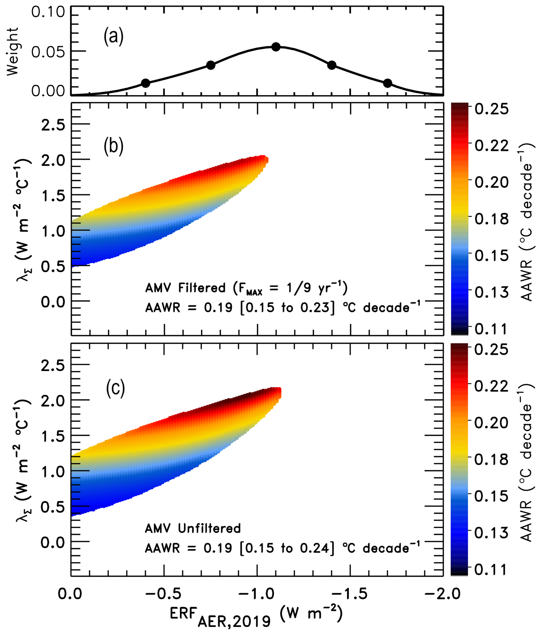
Figure 2 Aerosol weighting method, and computed values of AAWR for the EM–GC ensemble. (a) Asymmetrical Gaussian function used to weight the ensemble. The points marked on the Gaussian represent the center point, the 1σ and 2σ boundaries of the Gaussian (see Sect. 2.2.2 and Table S3 of Farago et al., 2025b). (b) Values of AAWR as the function of λ_Σ and ERF_AER,2019. Colors denote specific values of AAWR as indicated by the color bar on the right. AAWR is only shown for those combinations of λ_Σ and ERF_AER,2019, where all three χ² observational constraints are satisfied. The AMV input of the simulation used to produce this panel has been Fourier-filtered to remove frequencies greater than $\mathrm{1}/\mathrm{9}$ yr⁻¹ (see text). (c) As in (b), but without a Fourier-filter having been applied to the AMV input. The 50th percentile and the 5 %–95 % range of AAWR from the weighted ensemble are also given on panels (b) and (c).

The reconstruction of GMST and OHC over the training period is largely unaffected by the removal of the high-frequency component of the AMV input. As shown in Fig. 2b and c, the range of AAWR is similar between the two sets of simulations. The weighted central estimate and 5 %–95 % range for AAWR is 0.19 °C per decade [0.15 to 0.23 °C per decade], and 0.19 °C per decade [0.15 to 0.24 °C per decade] for the simulations where the AMV input was Fourier-filtered and unfiltered, respectively. Our estimates of AAWR, based on the 1975 to 2014 period, are generally consistent with Samset et al. (2023), who found the rate of warming to be 0.19 °C per decade between 1971 and 2020 using the HadCRUT5 dataset, with an acceleration in the rate of warming starting in 1990s. The values of AAWR shown here imply that a sizeable portion of the rise in GMST in the recent few years can be explained with the continued trend of anthropogenic GHG emissions. For example, the rate of 0.19 °C per decade corresponds to an increase in GMST of about 0.1 °C in 2024 relative to 2019. As a comparison, Gettelman et al. (2024) suggested that the IMO2020 regulations increase global temperatures by about 0.04 and 0.08 °C by 2023 and 2030, respectively, relative to 2020. Therefore, the change in GMST due to the IMO2020 regulations would correspond to only a few years of continued anthropogenic activity at the 1975 to 2014 rates. A similar comparison can be drawn with Jordan and Henry (2024), who found that IMO2020 increases global surface temperature by 0.046 °C in the 2020–2029 period, and concluded that temperature impact of IMO2020 corresponds to about 2–3 years' worth of continued global warming. Importantly however, such a rise in GMST due to IMO2020 corresponds to a significant acceleration of human-induced warming in the recent few years, which we address in Sect. 4.

3.2 Natural and anthropogenic contributions to recent temperature anomalies

Next, we quantify the contribution of various natural and anthropogenic factors to the GMST over the past half-decade. Figure 3 shows the modelled GMST for the Reference (left), IMO–0.1 (middle) and IMO–0.15 (right) simulations. The top panels of each column show the observed GMST anomaly from the HadCRUT5 dataset (black) and the EM–GC simulated range. Colors denote the EM–GC simulated cumulative probability of the GMST being greater or equal than a given value at a time, as indicated by the color bar to the right. The probabilities are obtained from weighting the EM–GC ensemble using an asymmetrical Gaussian function (Fig. 2a) as summarized in Sect. 2.1.2, and detailed in McBride et al. (2021) and Farago et al. (2025b). The shading represents the uncertainty range of simulated GMST, with the white line corresponding to the 50th percentile of simulated GMST, while the red and blue regions are associated with ensemble members of high and low climate sensitivities, respectively.

Panels (d)–(f) show the simulated rise in GMST due to IMO2020, based on global energy balance. Panels (g)–(r) show the simulated contributions of natural variability to the GMST, computed based on observed climate indices (Sect. 2.1 and 2.2). We will refer to these contributions shown in Fig. 3g–r as natural, with the understanding that some of these processes, and hence the corresponding climate indices, may have been influenced by external anthropogenic factors, including possibly even IMO2020.

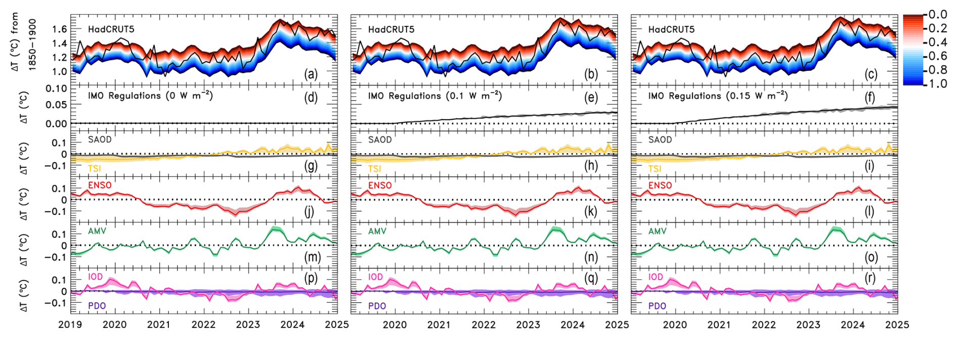
Figure 3 Probabilistic simulation of GMST and the contributions of various factors to GMST for the Reference (left), IMO–0.1 (middle) and IMO–0.15 (right) scenarios. Panels (a)–(c) show the EM–GC simulated GMST, with colors denoting the probability of the GMST being a given value, or greater, as indicated by the color bar on the right. The black line is the observed GMST from the HadCRUT5 dataset. All GMST anomalies are with respect to an 1850–1900 pre-industrial baseline. (d–f) Contribution of IMO2020 to the GMST anomaly based on global energy balance. (g–r) Contribution of natural factors (see text) to GMST. On panels (d)–(r), the solid line is the EM–GC median estimate (which we define as the 50 % probability), while the shading corresponds to the 5 %–95 % uncertainty range.

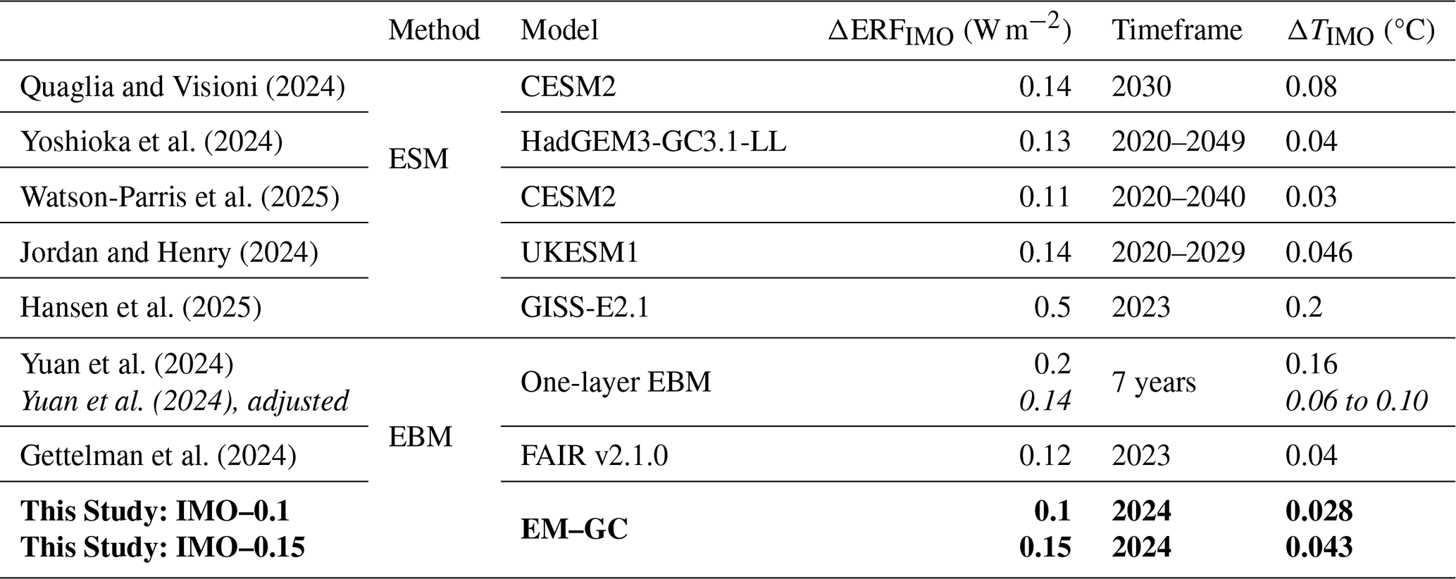
Table 1 summarizes our estimates of ΔT_IMO in response to changes in the global radiative forcing due to IMO2020 (ΔERF_IMO), as well as values from recently published studies. We find that the IMO2020 regulations increased GMST by 0.028 °C [0.025 to 0.031 °C, 5 %–95 % range] and 0.043 °C [0.038 to 0.046 °C] by the end of 2024 for the IMO–0.1 and IMO–0.15 scenarios, respectively. We refer to these quantities as ΔT_IMO, and we term this computed warming as being due to global energy balance, since these values have been quantified using the two-layer EBM component of our model. As noted above, additional localized effects from IMO2020 may be blended into the observed climate indices, upon which the contributions to changes in GMST shown in Fig. 3g–r are based. We briefly address this topic in Sect. 3.3.

Our estimates of ΔT_IMO under the IMO–0.1 and IMO–0.15 scenarios are consistent with values ΔT_IMO obtained both from EBMs (Gettelman et al., 2024) and ESMs (Jordan and Henry, 2024; Yoshioka et al., 2024; Watson-Parris et al., 2025) (Table 1). Studies provide estimates of ΔT_IMO over different time periods, as specified in Table 1. While the EBM-based estimates of Gettelman et al. (2024) were obtained using an EBM calibrated on CMIP6 model output, our results are based on an EBM trained on observational datasets. There are three studies that provide values of ΔT_IMO considerably larger than our estimates. Quaglia and Visioni (2024) estimate ΔT_IMO to be about 0.08 °C, a factor of 2 greater than our IMO–0.15 value of 0.043 °C [0.038 to 0.046 °C]. They also found significant warming in the North Atlantic, highlighting that localized effects of IMO2020 may be substantial. As noted above, a portion of the localized effects may be blended into the observational datasets that are used as our inputs. Consequently, the contributions of these localized effects to GMST, particularly for the North Atlantic, are not attributed to IMO2020 in the simulations presented in Fig. 3 and summarized in Table 1. Yuan et al. (2024) report a value of 0.16 °C for ΔT_IMO, a factor of two larger than the Quaglia and Visioni (2024) estimate. As highlighted by Watson-Parris et al. (2025), the estimate of ΔT_IMO provided in Yuan et al. (2024) is found using a global climate feedback parameter applied to an ERF perturbation over only the oceans. Consequently, Watson-Parris et al. (2025) suggest that the global value of ΔERF_IMO and ΔT_IMO should be lower than those presented in Yuan et al. (2024). Therefore, Table 1 includes the original values presented in Yuan et al. (2024) as well as the adjusted estimates provided by Watson-Parris et al. (2025). This adjusted value of 0.06 to 0.10 °C, in response to a ΔERF_IMO of 0.14 W m⁻², is among the higher estimates for ΔT_IMO. Finally, a recent study by Hansen et al. (2025) suggests a much higher value of ΔERF_IMO based on observations of absorbed solar radiation. Accordingly, their estimate of ΔT_IMO=0.2 °C is much higher than that reported in other studies, including ours, primarily due to their higher estimate of ΔERF_IMO. In our analysis, we focus on simulations with ΔERF_IMO being equal to 0.1 and 0.15 W m⁻², as the majority of the estimates for ΔERF_IMO currently available in literature are close to these values.

Table 1 Estimates of the change in global radiative forcing due to IMO2020 (ΔERF_IMO), and the corresponding change in global surface temperature (ΔT_IMO). For Yuan et al. (2024), we present the non-global values as published in their paper, as well as the globally scaled values (italic) suggested by Watson-Parris et al. (2025). Results from the EM-GC simulations presented in this paper are shown in bold.

Next, we quantify the contributions of various natural factors to GMST. We show the modelled contribution of ENSO to the GMST between 2019 and the end of 2024 in Fig. 3j–l. We find that the annual mean GMST in 2023 and 2024 increased by about 0.092 °C [0.049 to 0.120 °C, 5 %–95 % range] and 0.124 °C [0.079 to 0.150 °C] respectively, relative to 2022, as a consequence of a shift from La Niña to El Niño. The difference between the annual mean GMST anomaly in 2022 and 2023 is about 0.3 °C in the HadCRUT5 dataset. Therefore, about one third of the difference in GMST between 2022 and 2023 can be explained with the shift from La Niña to El Niño. Our results align well with the estimates of Goessling et al. (2025), who found that the onset of El Niño contributed about 0.07 °C to the temperature anomaly in 2023. Estimates for the contribution of ENSO to the 2023 and 2024 temperature anomalies were also provided by the State of the Global Climate 2024 report of the World Meteorological Organization (WMO) (WMO, 2025), hereafter WMO24. Using linear regression to the February/March Niño 3.4 index, WMO24 found that annual temperatures rose by about 0.08 °C in 2023 relative to 2022 due to ENSO (see their Datasets and methods section), which aligns quite well with our estimate of 0.092 °C for this period. However, WMO24 suggests that an additional increase of 0.12 °C in the annual global mean temperature between 2023 and 2024 can also be attributed to ENSO. We find the increase of GMST due to ENSO between 2023 and 2024 to be only 0.032 °C, which is much lower than the WMO24 estimate. Raghuraman et al. (2024) suggested that prolonged La Niña events may lead to sudden changes in the GMST of 0.25 °C or greater during the subsequent El Niño event, based on the analysis of several CMIP models. Conversely, our results do not indicate the occurrence of an ENSO-driven spike in GMST of the magnitude suggested in Raghuraman et al. (2024). Our conclusions regarding the influence of ENSO on the 2023 GMST anomalies align much better with those of Terhaar et al. (2025), who suggested that a strong El Niño event is a necessary, but not sufficient condition for the development of temperature spikes similar to that observed in 2023.

Starting in January 2023, a positive IOD event was also found to have influenced GMST (Fig. 3p–r). This IOD event contributed to a rise in GMST of 0.075 °C [0.036 to 0.096 °C, 5 %–95 % range] in 2023, relative to 2022. This positive IOD event persisted into early 2024, and gradually shifted to a negative phase by the end of 2024. In 2024, GMST was found to be 0.053 °C [0.019 to 0.074 °C] higher due to IOD, relative to 2022. Xie et al. (2025) suggested that while the co-occurrence Extreme Positive IOD (EXpIOD) events, such as the one observed in 2023, may be coincidental with the onset of El Niño, co-occurring El Niño and positive IOD events result in the amplification of the intensity of IOD. Our computation of the increase in GMST of 0.075 °C from 2022 to 2023 due to IOD is comparable in magnitude to ENSO's impact on the GMST between these two years (0.092 °C). Further discussion of the impact of IOD on GMST is given in Sect. 3.4.

Increased TSI due to the 11-year solar cycle also contributed to the observed rise in GMST in 2023 and 2024, relative to 2022 (Fig. 3g–i). In 2023 and 2024, the annual mean TSI was 0.35 and 0.40 W m⁻² higher than in 2022, respectively. This increase in TSI is found to have contributed to a rise in the annual mean GMST of 0.025 °C [−0.009 to 0.051 °C, 5 %–95 % range] and 0.029 °C [−0.008 to 0.056 °C] in 2023 and 2024, respectively, relative to 2022. Our central estimate of the contribution of TSI to GMST (0.025 °C) in 2023 aligns exceptionally well with the estimate of 0.027 °C found by Goessling et al. (2025), though we find a wider range of uncertainty at [−0.009 to 0.051 °C, 5 %–95 % range] in contrast to their range of [0.022 to 0.032 °C, 90 % confidence]. Our estimates for the impact of TSI on GMST are generally consistent with, albeit on the lower end of those of WMO24, who found the contribution of the changes in the solar cycle to GMST to be about 0.04 °C [0.015 to 0.065 °C, 95 % confidence] and 0.07 °C [0.045 to 0.095 °C] in 2023 and 2024, respectively. A similar analysis to that of WMO24 is given by Sect. S7 of Forster et al. (2025), hereafter F25, who suggested contributions from TSI to the GMST anomaly to be 0.03 °C [0.01 to 0.05 °C] and 0.04 °C [0.02 to 0.07 °C] in 2023 and 2024, respectively. Our estimates of the impact of TSI on GMST for these two years are in good agreement with the F25 values, both in terms of the central value and the range of uncertainty.

The contributions of SAOD and PDO to the GMST anomalies in 2023 and 2024 are found to be small relative to ENSO and IOD (Fig. 3g–i and p–r). The median estimates of the contribution of PDO to the modelled GMST are −0.008, −0.009 and −0.009 °C for the years 2022, 2023 and 2024, respectively. SAOD is found to be responsible for a slight cooling effect of −0.020, −0.023 and −0.015 °C in 2022, 2023 and 2024, respectively. As described in Sect. 2.2.4, for the simulations presented in this paper, we neglected the injection of water vapor into the stratosphere from the eruption of Hunga. Nevertheless, our SAOD-based proxy for volcanic activity leads to an estimated −0.023 °C cooling in 2023, in line with the values of −0.02 °C [−0.01 to −0.03 °C] presented in WMO24 and F25. Therefore, the neglect of the injection of water vapor from Hunga appears to have no major consequence on our results.

3.3 North Atlantic warming

We now discuss the contribution of AMV and North Atlantic SST anomalies to the GMST in 2023 and 2024 (Fig. 3m–o). Multiple recent studies have highlighted the unusually high SST anomalies in the North Atlantic (Kuhlbrodt et al., 2024; Carton et al., 2025; England et al., 2025; Guinaldo et al., 2025; Dong et al., 2025), alongside reduced low-cloud cover in the region during 2023 (Goessling et al., 2025; Tselioudis et al., 2025). Gettelman et al. (2024) suggested that the resulting increase in local temperatures due to IMO2020 may be much greater than implied by the EBM-based global values, particularly in the Northern Hemisphere mid-latitude oceans. Similarly, Quaglia and Visioni (2024) found a considerable rise in the surface air temperature in the North Atlantic due to IMO2020. While a global EBM, such as our EM–GC, cannot directly be used to study localized temperature anomalies, a few key conclusions can still be drawn, as described below.

The variability in North Atlantic SSTs is represented by our AMV index, which we obtained by detrending the time series of area weighted North Atlantic SSTs using the magnitude of global anthropogenic ERF (Sect. 2.2.5). The contribution of AMV to GMST has shown a generally steady increase since 2019, with a particularly large contribution in the second half of 2023 (Fig. 3m–o). AMV is found to have contributed 0.053 °C [0.044 to 0.068 °C, 5 %–95 % range] and 0.052 °C [0.045 to 0.065 °C] to the annual mean GMST in 2023 and 2024, respectively. The modelled contribution of AMV to the GMST anomaly in 2022 is slightly negative, at −0.017 °C [−0.010 to −0.026 °C]. Consequently, an increase in GMST of about 0.070 °C from 2022 to 2023 is attributed to AMV in our model framework, which is on the scale of the ENSO and IOD-related rise in GMST between the same two years. The impact of AMV on the GMST anomaly in 2024 relative to 2022 is about 0.069 °C.

The peak in our AMV index (and therefore, the contribution of this proxy to GMST in Fig. 3m–o) in mid-late 2023 is consistent with the record high observed North Atlantic SSTs in 2023 (Carton et al., 2025; Guinaldo et al., 2025). Samset et al. (2024) also found that conditions in the North Atlantic contribute strongly to the global temperatures in 2023, using a Green's function-based method. They estimated that SSTs in the subtropical and tropical North Atlantic contributed about 0.02 and 0.04 °C to the annual mean global surface temperature anomaly in 2023. These values are generally in line with our estimates derived from the AMV index noted in the prior paragraph.

Next, we analyze whether the substantial contributions from AMV in our simulations originate from long-term trends, or short-term variability. We perform the same analysis that was shown in Sect. 3.2 with a second set of simulations, where the high-frequency component of the AMV index, that is, frequencies greater than $\mathrm{1}/\mathrm{9}$ yr⁻¹, is removed using a Fourier filter (Sect. 2.2.5). The regression to the historical GMST and OHC during the model training period of 1850 to 2019 is largely unaffected by the choice of AMV input (Sect. 3.1). Figure 4 shows the EM–GC simulations that use a Fourier-filtered AMV input for the Reference, IMO–0.1 and IMO–0.15 scenarios in a manner similar to Fig. 3. The contributions of all factors to the GMST shown in Fig. 4g–r are highly similar to those in Fig. 3g–r, except for the contributions of AMV. The contribution of AMV to the annual mean GMST is found to be 0.008 °C higher in 2023 relative to 2022, due to a slow rising trend in the AMV index (Fig. 4m–o). This value, however, is nine times smaller than that quantified from simulations where the AMV input was not Fourier-filtered. Further, the simulated GMST shown in Fig. 4a–c is lower than the observations in mid-late 2023 and late 2024. For both of these time periods, there is a substantial AMV contribution to GMST when the AMV index has not been Fourier-filtered (Fig. 3m–o), which is absent in simulations that use Fourier-filtered AMV input (Fig. 4m–o). Consequently, our simulations imply that short-term variability in the North Atlantic SSTs was likely a strong contributor to the observed GMST anomalies in late 2023 and 2024.

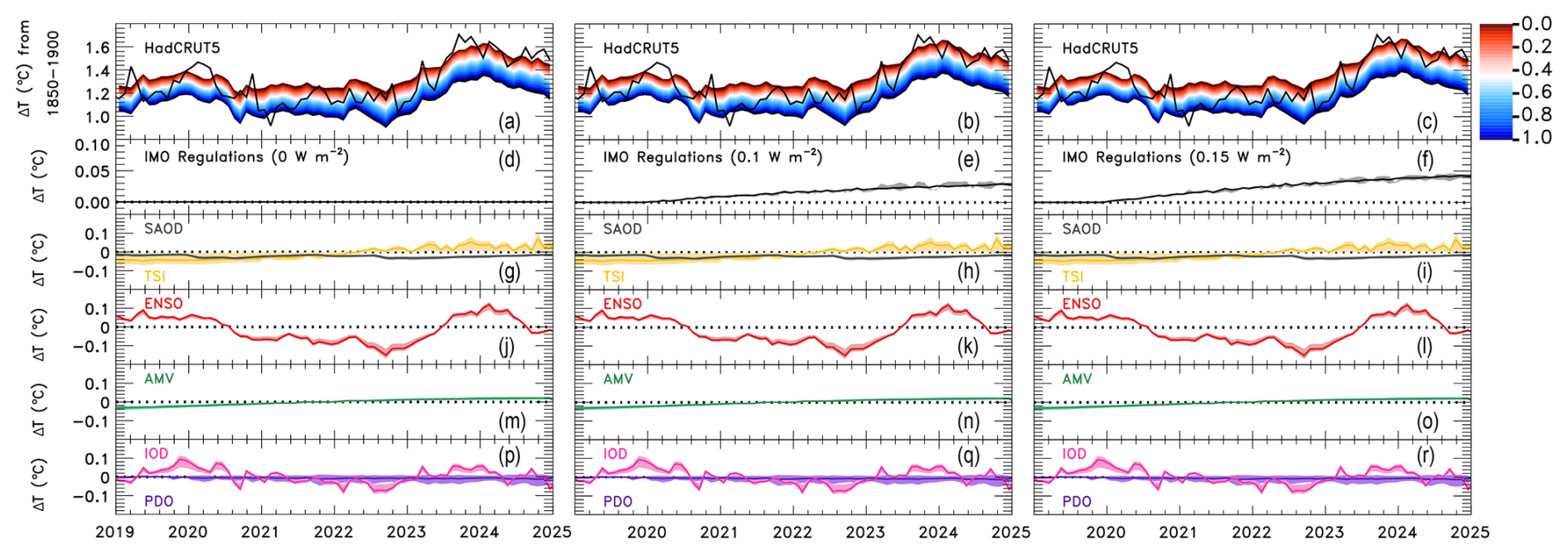
Figure 4 Probabilistic simulation of GMST and the contribution of various factors for the Reference (left), IMO–0.1 (middle) and IMO–0.15 (right) scenarios. As in Fig. 3, except that the input time series for AMV has been Fourier-filtered to remove frequencies greater than $\mathrm{1}/\mathrm{9}$ yr⁻¹ (see text).

Establishing a connection between the high North Atlantic SSTs and the IMO2020 regulations remains challenging. In our model framework, we detrended the AMV index using the time series of global anthropogenic radiative forcing, following Sect. 3.2.3 of Canty et al. (2013). Local anomalies in ERF that exceed the global values would result in parts of the AMV index carrying an additional, localized anthropogenic component. Consequently, localized effects of IMO2020 may be blended into the AMV index, which would correspond to the impact of IMO2020 on GMST to be greater than implied solely by the global energy balance approach. If we assume that the short-term variability in North Atlantic SSTs described above is driven primarily by IMO2020, than an additional 0.06 °C in the increase in GMST from 2022 to 2023 can be attributed to IMO2020, which result in estimates of ΔT_IMO that align quite well with those of Quaglia and Visioni (2024) (Table 1).

Watson-Parris et al. (2025) reported that IMO2020 produces a pattern of North Atlantic SSTs that is similar to those observed in 2023 in CESM2, but only after about 20 years, and no significant warming in this region is simulated between 2020 and 2025. This result contradicts Quaglia and Visioni (2024), who found notable warming in the North Atlantic over the 2021–2023 period with the CESM2 model. As highlighted in Watson-Parris et al. (2025), different experimental setups account for some of the differences between ESM-based results that investigate the effects of IMO regulations. Jordan and Henry (2024) report lower cloud albedo in the North Atlantic due to IMO2020, which aligns with the observed albedo described in Goessling et al. (2025). Consequently, Jordan and Henry (2024) suggest that the increase in ERF due to IMO2020 is about 2.5 times greater in the North Atlantic region than the value of the global mean. Meanwhile, Carton et al. (2025) attributed the record high SSTs to a combination of increased downwelling radiation, as well as reduced latent and sensible heat loss due to lower trade wind speeds. Carton et al. (2025) and Guinaldo et al. (2025) also highlighted that a considerable preconditioning effect in the North Atlantic also played a significant role in the development of the SST anomalies observed in 2023. England et al. (2025) attributed the anomalously high SSTs in the region during the summer of 2023 primarily to low wind speeds and a record-low mixed layer depth (MLD), partly due to a steady decline in MLD in recent decades. England et al. (2025) thus found the IMO regulations to have been minor contributors to the high SST anomalies over this period. Similarly, Guinaldo et al. (2025) suggested that the high SST anomalies in the region are a result of a rare event of internal variability at the current levels of global warming. Overall, studies vary in their estimates of how much of the warming in the North Atlantic region is directly attributable to the IMO2020 regulations. Our results suggest that short-term variability in the North Atlantic SSTs was responsible for a portion of the observed rise in GMST between 2022 and 2023, but whether the effects of the IMO2020 regulations could be mistaken for variability remains unclear.

3.4 Indian Ocean Dipole

We conclude with some additional comments on the contributions of the IOD to the anomalously high value of GMST observed in 2023. During positive phases of IOD (pIOD) warm surface air conditions are observed in parts of Australia, Africa, Asia, South America and Europe (Saji and Yamagata, 2003; Saji et al., 2005; IPCC, 2021a; Andrian et al., 2024). Furthermore, IOD exhibits a positive skewness: that is, positive IOD events tend to have a stronger amplitude than negative events (Hong et al., 2008; Cai et al., 2012; Ogata et al., 2013; Cai and Qiu, 2013; Ng and Cai, 2016; An et al., 2023). In our model framework, we find a significant contribution of IOD to the high GMST anomaly in 2019 (Fig. 3p–r). The strong pIOD event in 2019 has been associated with the unusually hot and dry conditions in Southeastern Australia, that led to devastating wildfires in late 2019 (Wang and Cai, 2020).

El Niño and pIOD events often co-occur (e.g. Sun et al., 2022), such as in 2019 and 2023, and isolating the effects of IOD events from ENSO is challenging (Saji and Yamagata, 2003; Andrian et al., 2024). Here, we perform a simple correlation analysis between the surface air temperatures and IOD to provide a qualitative illustration of the effects of the 2023 ExpIOD on regional temperatures (Figs. S7–S9). In this section, we focus on the main conclusions of this correlation analysis, and provide a more detailed description of this analysis in our Supplement. We examined the correlation between the annual mean surface air temperature from the ERA5 reanalysis (Hersbach et al., 2020) and the COBE2 IOD index used in our simulations (Fig. S7a) over 1980–2024. We highlight four geographic regions (black boxes on Figs. S7–S9), where the correlation between annual mean surface air temperatures and ENSO is limited (Fig. S9), but the correlation with IOD is high (Fig. S7a–b). These four regions are generally consistent with locations of high IOD influence described in prior literature (Saji and Yamagata, 2003; Saji et al., 2005; IPCC, 2021a; Andrian et al., 2024). As shown in Fig. S7c, these four regions experienced a considerable rise in the annual mean surface temperature in 2023 (positive IOD) relative to 2022 (negative IOD). In 2024 (neutral IOD), these regions experienced cooler, or similar surface temperatures relative to 2023. We repeated this correlation analysis for the August–October (ASO) season (Fig. S8), which corresponds to the largest 3-month mean contribution to GMST from IOD in 2023 (Fig. 3p–r). During the ASO season, all of the highlighted regions experienced a significant rise in surface temperatures in 2023 relative to 2022, and a subsequent decline in 2024 (Fig. S8c–d). This simplified correlation analysis reinforces our suggestion that the ExpIOD event in 2023 provided a significant contribution to the unusually high temperatures experienced that year. Further evaluation of this conclusion will require Earth System modelling that accounts for the various climatological impacts of strongly positive IOD events.

Table 2 Modelled 50th percentile contributions of various anthropogenic and natural factors to the rise in annual mean GMST in 2023 and 2024 relative to 2022, for the IMO–0.15 scenario. The columns labelled “Without IOD” correspond to simulations where the IOD was removed as a regressor from the model simulations. The sum of the individual contributions, as well as the observed GMST anomaly from HadCRUT5, is shown in bold, while the difference between the modelled and observed GMST is given in italic.

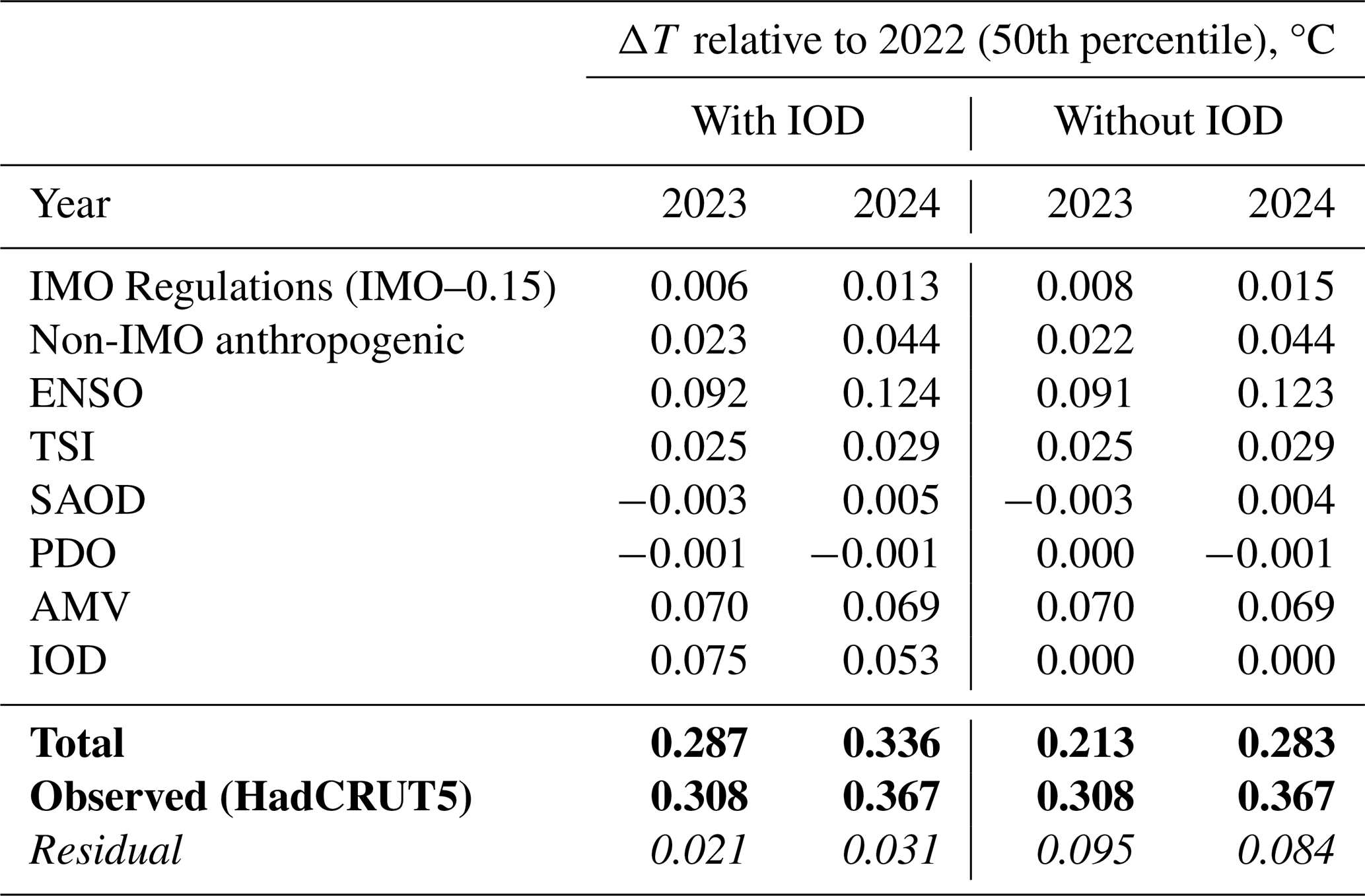
Next, we provide a summary of the contributing factors to the GMST anomalies observed in 2023 and 2024. Table 2 shows the 50th percentile contributions of natural and anthropogenic factors to the rise in the annual mean GMST in 2023 and 2024 relative to the year 2022, for the IMO–0.15 scenario. We also show results from a second set of simulations, labeled “Without IOD” in Table 2, where IOD was removed as a regressor from the model. The removal of IOD as a regressor has virtually no impact on the contributions of the other factors, but results in an underrepresentation of the GMST during ExpIOD events, such as in 2023, as shown by the residuals given in Table 2. Other recent analyses of the factors that led to the record warmth in 2023 and 2024, such as WMO24 and F25, did not consider possible contributions from IOD. A reconstruction of the 2023 GMST anomaly given by WMO24 and F25 falls short of the observed anomaly by about 0.09 °C. In contrast, their reconstructions of the 2024 GMST anomaly are in much better agreement with the observations. The impact of IOD highlighted in Table 2 may reconcile the gap between the estimated and observed GMST for 2023 reported by WMO24 and F25.

Finally, we compare the IOD-related rise in annual mean GMST from 2022 to 2023 to IOD events of the past. Over the 1851–2019 time period, IOD explains only a small fraction of the variability in GMST (R²=0.027, Fig. S1a). However, the rise in IOD between 2022 and 2023 is nearly unprecedented since 1850. Figure S10 shows a scatterplot of the rise in the annual mean value of the IOD index relative to the previous year, computed from two separate IOD indices that differ in the underlying SST datasets: the COBE2 IOD index used for the simulations of this paper (horizontal axis), and the NOAA DMI IOD index (vertical axis), which is based on HadISST SSTs (Sect. 2.2.3). The shaded areas in Fig. S10 represent the highest 5th percentile values of these IOD anomalies. Only three years fall into the 5th percentile of both datasets: 1961, 2017, and 2023. The rise in IOD from 2022 to 2023 is the highest on record for the COBE2 index, and the second highest in the NOAA DMI index. To test the sensitivity of our conclusions to the choice of IOD dataset, we performed a model simulation that uses the NOAA DMI index as the input for IOD. The contributions of natural and anthropogenic factors to the GMST obtained from this simulation are given in Table S1 in the Supplement, in a manner similar to Table 2. Using the NOAA DMI index as the input for IOD, the rise in GMST from 2022 to 2023 that is associated with IOD was found to be 0.072 °C [0.004 to 0.105 °C, 5 %–95 % range], which is highly similar to the values found using the COBE2 index of 0.075 °C [0.036 to 0.096 °C]. Consequently, our conclusion regarding the contribution of IOD to the rise in GMST between 2022 and 2023 is largely independent of the choice of IOD dataset. Additional analysis of the contributions of other factors for the model run that is based on the NOAA DMI Index is provided in the Supplement.

Figure S10 highlights the nearly unprecedented rise in IOD from 2022 to 2023. Understanding the mechanisms of such a strong shift in the IOD is beyond the scope of this paper. However, the amplifying effect of a co-occuring strong El Niño event may have been a strong contributor to the conditions in the Indian Ocean that led to the development of this pIOD event, as suggested by Xie et al. (2025). In addition, as described above, the spatial pattern of surface temperature anomalies observed in 2023 resembles patterns similar to those associated with strong IOD events over the past half century.

4 Conclusions

Several factors may have contributed to the observed temperatures exceeding expectations in 2023 and 2024. In this paper, we use a multiple linear regression energy balance model (EM–GC) to quantify the influence of various natural and anthropogenic factors on the GMST in these years, including the reduction of sulfate emissions from international shipping starting in 2020. Our model is trained on 170 years of historical GMST data and 65 years of OHC measurements, and uses observed climate indices to simulate the impact of internal variability on GMST, thereby providing a quantification of warming due to various natural and anthropogenic factors. Therefore, our simulations provide observation-driven estimates of the GMST anomaly in 2023 and 2024, and serve as a complementary modelling effort to simulations performed with ESMs, as well as EBMs calibrated using CMIP model output.

The annual human-induced rate of rise in GMST between 2022 and 2024 (without the effects of the IMO regulations) was found to be about 0.022 °C yr⁻¹, which corresponds to a decadal rate of 0.22 °C per decade (Table 2). In contrast, the anthropogenic warming rate over 1975–2014 was found to be 0.19 °C per decade (Sect. 3.1). The difference between these two rates is consistent with the acceleration of human-induced warming in this century (e.g. Samset et al., 2023, 2025).

We simulate the response of GMST to increases in ERF due to IMO2020 (ΔERF_IMO) of +0.1 and +0.15 W m⁻², which were chosen to be close to recent estimates of ΔERF_IMO available in literature. We find that the IMO2020 regulations are responsible for an increase in GMST (ΔT_IMO) of 0.028 °C [0.025 to 0.031 °C, 5 %–95 % range] and 0.043 °C [0.038 to 0.046 °C] from the start of 2020 to the end of 2024 for these two cases, respectively. These values of ΔT_IMO are in line with several other recent estimates (Jordan and Henry, 2024; Yoshioka et al., 2024; Watson-Parris et al., 2025; Gettelman et al., 2024). Importantly, the IMO–0.15 case corresponds to an additional acceleration of human-induced warming by about 0.006 °C yr⁻¹ over 2023–2024 (Table 2). This value is about 30 % of the GHG-driven anthropogenic rate, suggesting that the IMO2020 regulations may be responsible for a considerable rise in the rate of human-induced warming since 2020. Therefore, while the rise in GMST attributable to the IMO2020 regulations likely corresponds to only a few years of global warming based on recent trends, this factor is found to have increased the rate of human-induced warming by up to 30 % since 2020.

We also find that GMST increased by about 0.092 °C from 2022 to 2023 due to the shift from La Niña to El Niño conditions, which explains about one third of the observed rise in GMST between these two years. About 0.070 °C [0.054 to 0.094 °C] of the rise in GMST from 2022 to 2023 is attributed to AMV; this value is considerably lower, only 0.008 °C [−0.002 to 0.018 °C], when the high-frequency component of the AMV index is removed. We find that the removal of the high-frequency component of the AMV index leads to an underrepresentation of GMST in mid-late 2023 and late 2024, which suggests that short-term variability in the North Atlantic SSTs may have been a significant factor that influenced the GMST anomalies observed in 2023 and 2024. Whether these changes in North Atlantic SSTs are a direct result of the introduction of the IMO2020 regulations remains unclear; better understanding of the internal and external drivers of North Atlantic SSTs is required to make a definitive attribution. Finally, our analysis suggests an additional contribution to the annual mean GMST anomalies in 2023 and 2024 (both relative to 2022) of 0.075 °C [0.036 to 0.096 °C] and 0.053 °C [0.019 to 0.074 °C], respectively, due to a strong positive Indian Ocean Dipole event (Sect. 3.4). Our study is the first to suggest a significant contribution from the Indian Ocean Dipole to the anomalously high values of GMST observed in 2023 and 2024.

Appendix A: Two Layer Energy Balance Module

A1 Implementation of EBM–1 in EM–GC

The two-layer approximation separates the climate system into two layers, an upper layer of small heat capacity, representing the well-mixed layer of oceans, as well as the land and the atmosphere, and the lower layer, which corresponds to the deeper layers of Earth's oceans. The atmosphere and the land are assumed to have a negligible heat capacity relative to that of the oceans, and therefore, the states of the upper and lower layers are described by Eqs. (A1) and (A2), respectively (Geoffroy et al., 2013a, b). The exact mathematical formulation that describes the states of the two layers in the two-layer EBM differs between studies. Here and throughout, our formulation is based on Eqs. (1) and (2) of Geoffroy et al. (2013a).

$$\begin{array}{}\text{(A1)}& {\displaystyle }{C}_{\mathrm{u}}{\displaystyle \frac{\mathrm{d}{T}_{\mathrm{u}}}{\mathrm{d}t}}=F-\mathit{\alpha }{T}_{\mathrm{u}}-\mathit{\gamma }\mathit{\epsilon }(T_{\mathrm{u}}-T_{\mathrm{d}})\text{(A2)}& {\displaystyle }{C}_{\mathrm{d}}{\displaystyle \frac{\mathrm{d}{T}_{\mathrm{d}}}{\mathrm{d}t}}=\mathit{\gamma }(T_{\mathrm{u}}-T_{\mathrm{d}})\end{array}$$

In Eqs. (A1) and (A2), T_u and T_d (units of K) represent the temperature anomalies of the upper, and the lower layer, respectively, relative to pre-industrial conditions. The quantities C_u and C_d are the effective heat capacities of the upper and lower layers per unit area (in units of J m⁻² K⁻¹), respectively. The quantity F is the effective radiative forcing of the climate (units of W m⁻²) relative to pre-industrial conditions, while α is the climate feedback parameter (in W m⁻² K⁻¹). The quantity γ is the heat transport coefficient between the two layers of the ocean (in W m⁻² K⁻¹). The dimensionless parameter ε represents the efficacy of the deep ocean heat uptake (Geoffroy et al., 2013a, b). The two-layer EBM described by Eqs. (A1) and (A2) is commonly termed EBM−ε.

The EBM−ε representation can be simplified using the assumption that ε=1 (Geoffroy et al., 2013b). This simplification leads to the formulation commonly referred to as EBM–1. As shown in Geoffroy et al. (2013b), the EBM–1 representation provides a highly similar temperature response to EBM−ε on the timescale of our simulations, but requires the calibration of one less parameter. Therefore, we implemented the EBM–1 representation into EM–GC and have assumed that ε=1 throughout this paper. Equations (A1) and (A2) are converted to a monthly time grid to match the temporal resolution of EM–GC as described below, and are then used to express the temperature anomalies of the upper (T_u) and lower ocean layers (T_d). We consider the time series of the temperature anomaly of the upper layer (T_u) to be equal to ΔT_ANTH in Eq. (1). This treatment of OHE is consistent with earlier versions of the EM–GC model, which also assumed that the warming of the climate and the oceans are primarily driven by anthropogenic activity.

Internally, EM–GC uses a time-invariant climate feedback parameter λ_Σ, which is the sum of all feedbacks (water vapor, lapse rate, clouds, etc.), except for the Planck-feedback (McBride et al., 2021; Farago et al., 2025b). The quantity λ_Σ relates to the climate feedback parameter α in Eq. (A1) such that $\mathit{\alpha }={\mathit{\lambda }}_{\mathrm{p}}-{\mathit{\lambda }}_{\mathrm{\Sigma }}$, where λ_p is the response of a black body to a perturbation in the absence of climate feedback (Bony et al., 2006), and has the value of λ_p=3.2 W m⁻² K⁻¹ (McBride et al., 2021).

To convert Eqs. (A1) and (A2) to a monthly timescale, we use the backward Euler method, which assumes that the change in the temperature anomalies between two timesteps (ΔT_u and ΔT_d for the upper and lower layers, respectively) are expressed as shown in Eq. (A3). We use the backward Euler method because this formulation is less sensitive to the size of the timestep and reduces numerical instability for stiff differential equations.

$$\begin{array}{}\text{(A3)}& \begin{array}{rl}& {\displaystyle \frac{\mathrm{d}{T}_{\mathrm{u}}}{\mathrm{d}t}}={\displaystyle \frac{\mathrm{\Delta }{T}_{\mathrm{u}}}{\mathrm{\Delta }t}}={\displaystyle \frac{\left(T_{\mathrm{u},i}-T_{\mathrm{u},i-\mathrm{1}}\right)}{\mathrm{\Delta }t}}\text{ and}\\ & {\displaystyle \frac{\mathrm{d}{T}_{\mathrm{d}}}{\mathrm{d}t}}={\displaystyle \frac{\mathrm{\Delta }{T}_{\mathrm{d}}}{\mathrm{\Delta }t}}={\displaystyle \frac{\left(T_{\mathrm{d},i}-T_{\mathrm{d},i-\mathrm{1}}\right)}{\mathrm{\Delta }t}}\end{array}\end{array}$$

Consequently, Eqs. (A1) and (A2) are expressed on a monthly grid as shown in Eqs. (A4) and (A5), where i is the index of a given month, and Δt represents the length of each month, in units of seconds.

$$\begin{array}{}\text{(A4)}& {\displaystyle }{C}_{\mathrm{u}}(T_{\mathrm{u},i}-T_{\mathrm{u},i-\mathrm{1}}){\displaystyle \frac{\mathrm{1}}{\mathrm{\Delta }t}}=F_i-\mathit{\alpha }{T}_{\mathrm{u},i}-\mathit{\gamma }(T_{\mathrm{u},i}-T_{\mathrm{d},i})\text{(A5)}& {\displaystyle }{C}_{\mathrm{d}}(T_{\mathrm{d},i}-T_{\mathrm{d},i-\mathrm{1}}){\displaystyle \frac{\mathrm{1}}{\mathrm{\Delta }t}}=\mathit{\gamma }(T_{\mathrm{u},i}-T_{\mathrm{d},i})\end{array}$$

Rearranging Eqs. (A4) and (A5) to express the temperature anomalies of the upper and lower layers at a given time (T_u,i and T_d,i, respectively) yields Eqs. (A6) and (A7):

$$\begin{array}{}\text{(A6)}& {\displaystyle }{T}_{\mathrm{u},i}={\displaystyle \frac{F_i+\mathit{\gamma }{T}_{\mathrm{d},i}+\frac{C_{\mathrm{u}}}{\mathrm{\Delta }t}{T}_{\mathrm{u},i-\mathrm{1}}}{\left(\frac{C_{\mathrm{u}}}{\mathrm{\Delta }t}+\left(\mathit{\alpha }+\mathit{\gamma }\right)\right)}}\text{(A7)}& {\displaystyle }{T}_{\mathrm{d},i}={\displaystyle \frac{\mathit{\gamma }{T}_{\mathrm{u},i}+\frac{C_{\mathrm{d}}}{\mathrm{\Delta }t}{T}_{\mathrm{d},i-\mathrm{1}}}{\left(\frac{C_{\mathrm{d}}}{\mathrm{\Delta }t}+\mathit{\gamma }\right)}}\end{array}$$

The expression of T_u,i in Eq. (A6) includes the value of T_d,i; similarly, the T_d,i in Eq. (A7) is a function of T_u,i. We define the values of C_u and C_d prior to the beginning of the simulation (see Sect. A3), while the time series of effective radiative forcing, F(t) and the climate feedback parameter α are considered using an ensemble method (Sect. 2.1.2). For each ensemble member, the value of the parameter γ is quantified based on the observed rise in OHC (Sect. A2). Using these values for γ, the model then computes time series for T_u and T_d. This feature is highly similar to earlier versions of the EM–GC ocean module (Hope et al., 2020; McBride et al., 2021; Farago et al., 2025b), where a given value of the ocean heat transfer parameter defined the temperature anomaly time series of the upper layer of oceans for a specific ensemble member. A key difference between the updated two-layer EBM component in comparison to previous versions of EM–GC, is that in earlier versions of EM–GC, the temperature of the upper layer was computed such that a fixed percentage of total OHC is retained in the upper layer of the oceans. Consequently, earlier versions of our model resulted in an immediate jump in modelled GMST when a step-forcing was applied, similar to the behavior of the “deep-layer model” formulation described in Gregory et al. (2015), thereby overestimating the short-term temperature response to sudden increases in ERF. The two-layer EBM component presented here improves the energy balance component of EM–GC to provide a more realistic short-term response to sudden changes in radiative forcing, while retaining the concept of the iterative loop used to quantify the ocean heat transfer parameter based on observations, that was used in earlier versions of the EM–GC model (Hope et al., 2020; McBride et al., 2021; Farago et al., 2025b). We present the observation-driven calibration of the ocean heat transfer parameter γ in Sect. A2.

To compute T_u,i from Eqs. (A6) and (A7), we substitute T_d,i from Eq. (A7) into Eq. (A6), which we then rearrange to express T_u,i as shown in Eq. (A8).

$$\begin{array}{}\text{(A8)}& T_{\mathrm{u},i}={\displaystyle \frac{F_i+\frac{C_{\mathrm{u}}}{\mathrm{\Delta }t}{T}_{\mathrm{u},i-\mathrm{1}}+\frac{\mathit{\gamma }\frac{C_{\mathrm{d}}}{\mathrm{\Delta }t}{T}_{\mathrm{d},i-\mathrm{1}}}{\left(\frac{C_{\mathrm{d}}}{\mathrm{\Delta }t}+\mathit{\gamma }\right)}}{\left(\frac{C_{\mathrm{u}}}{\mathrm{\Delta }t}+\left(\mathit{\alpha }+\mathit{\gamma }\right)-\frac{{\mathit{\gamma }}^{\mathrm{2}}}{\left(\frac{C_{\mathrm{d}}}{\mathrm{\Delta }t}+\mathit{\gamma }\right)}\right)}}\end{array}$$

The expression of T_u,i shown in Eq. (A8) is only affected by various constants (γ, C_u, C_d, α and Δt), the value of radiative forcing in a given month (F_i), and the temperature anomalies of the upper and lower layers in the previous month ($T_{\mathrm{u},i-\mathrm{1}}$ and $T_{\mathrm{d},i-\mathrm{1}}$, respectively). Using the initial conditions of $T_{\mathrm{u}}(t=\mathrm{0})=T_{\mathrm{d}}(t=\mathrm{0})=\mathrm{0}$ K, and $F(t=\mathrm{0})=\mathrm{0}$ W m⁻², which correspond to the unperturbed state of the pre-industrial climate, the model computes the time series of T_u, which is then substituted into Eq. (A7) to obtain the time series of T_d for a given value of the parameter γ. For the simulations presented in the main paper, we use values of 7.3 and 106 $\mathrm{W}\mathrm{yr}{\mathrm{m}}^{-\mathrm{2}}{\mathrm{K}}^{-\mathrm{1}}$ for C_u and C_d, respectively, which correspond to equivalent ocean depths of 77 and 1105 m. These depths are the multi-model mean values, obtained by Geoffroy et al. (2013b) by fitting the two-layer EBM to the temperature output of a set of CMIP5 models. We describe the testing of the sensitivity of our model setup to the specific values of C_u and C_d in Sect. A3.

A2 Quantification of the ocean heat transfer parameter γ

Here, we present the calibration of the ocean heat transfer parameter γ within the EBM–1 component of EM–GC, using the observed rise in GMST and OHC. Our calibration is different from the common method for the calibration of the two-layer EBM, which uses CMIP5/6 simulations, where the concentration of CO₂ is abruptly quadrupled (hereafter termed abrupt4xCO₂ simulations) (Geoffroy et al., 2013a, b; Smith et al., 2021b).

In earlier versions of the EM–GC model (Hope et al., 2020; McBride et al., 2021; Farago et al., 2025b), the ocean heat transfer parameter, which was termed κ in these papers, was quantified based on the observed rise in OHC, using an iterative cycle between the value of κ, and the temperature of the well-mixed layer of the ocean. The calibration of EBM–1 described here follows the same logic: the model runs an iterative cycle between the value of the parameter γ, and the pair of temperature anomaly time series T_u and T_d. The heat capacities of the upper and lower layers (C_u and C_d, respectively) are pre-defined at the beginning of the simulation. We describe the setup of these two parameters in Sect. A3.

The observed rise in OHC over a given period can be approximated using the slope of a linear fit to the observed OHC record (Ocean Heat Export, OHE) following Canty et al. (2013). Similar to C_u and C_d, OHE is also expressed per unit area of the oceans, and has the dimension of W m⁻². The iterative cycle finds the value of the parameter γ that corresponds to the best match between the modelled and observed rise in OHC over the period where OHC data are available, as shown in Eq. (A9). In Eq. (A9), start and finish correspond to the first and last months of OHC data availability during the training period (1850 to 2019) of the model. In this paper, we use OHC data starting in 1955, and therefore, start and finish correspond to January 1955 and December 2019, respectively. The quantity tspn is the difference in time between start and finish, in the units of seconds.

$$\begin{array}{}\text{(A9)}& \underset{\mathrm{start}}{\overset{\mathrm{finish}}{\int }}\left(C_{\mathrm{u}}{\displaystyle \frac{\mathrm{d}{T}_{\mathrm{u}}}{\mathrm{d}t}}+C_{\mathrm{d}}{\displaystyle \frac{\mathrm{d}{T}_{\mathrm{d}}}{\mathrm{d}t}}\right)\mathrm{d}t=\text{OHE}\times tspn\end{array}$$

By substituting Eq. (A2) into Eq. (A9), we obtain Eq. (A10), which is then rearranged and converted to a monthly timescale to yield the expression of γ shown in Eq. (A11).

$$\begin{array}{}\text{(A10)}& {\displaystyle }\underset{\mathrm{start}}{\overset{\mathrm{finish}}{\int }}\left(C_{\mathrm{u}}{\displaystyle \frac{\mathrm{d}{T}_{\mathrm{u}}}{\mathrm{d}t}}+\mathit{\gamma }(T_{\mathrm{u}}-T_{\mathrm{d}})\right)\mathrm{d}t=\text{OHE}\times tspn\text{(A11)}& {\displaystyle }\mathit{\gamma }={\displaystyle \frac{\text{OHE}\times tspn-C_{\mathrm{u}}\times \sum _{\mathrm{start}}^{\mathrm{finish}}(T_{\mathrm{u},i}-T_{\mathrm{u},i-\mathrm{1}})}{\sum _{\mathrm{start}}^{\mathrm{finish}}\left(\left(T_{\mathrm{u},i}-T_{\mathrm{d},i}\right)\times \mathrm{\Delta }t\right)}}\end{array}$$

An initial value of γ (γ_INITIAL=1.05 W m⁻² K⁻¹) is used to compute the pair of T_u–T_d time series using Eqs. (A6) and (A7), which are then inserted into Eq. (A11) to obtain a new value of γ. This iterative loop continues until a convergence is reached, or until the model fails to find a value of γ that is consistent with observed rise in OHC. Equation (A11) serves as an extension of Eq. (5) from McBride et al. (2021), and allows the quantification of the ocean heat transfer parameter γ within the updated two-layer EBM module of EM–GC, based on the observed rise in OHC.

EM–GC simulations are constrained by the model's ability to reproduce the observed rise in OHC through the use of a reduced chi-square metric, termed ${\mathit{\chi }}_{\mathrm{OCEAN}}^{\mathrm{2}}$. We compute ${\mathit{\chi }}_{\mathrm{OCEAN}}^{\mathrm{2}}$ by using the time series of modelled and observed OHC in the upper 700 m of oceans, shown by the red and black lines in Fig. 1g, respectively. Similarly to earlier versions of the EM–GC model (Hope et al., 2020; McBride et al., 2021; Farago et al., 2025b), the total modelled OHC (left side of Eq. A10) in EM–GC is scaled to 70 % of its value to obtain the modelled OHC in the upper 700 m of oceans, using the assumption that the upper 700 m of oceans hold 70 % of the heat (IPCC, 2007). This ratio is broadly consistent with Table 2.7 of the IPCC AR6 report (Gulev et al., 2021), which estimated that about 66 % of total OHC was held in the upper 700 m of oceans over the 1901 to 2018 time period.

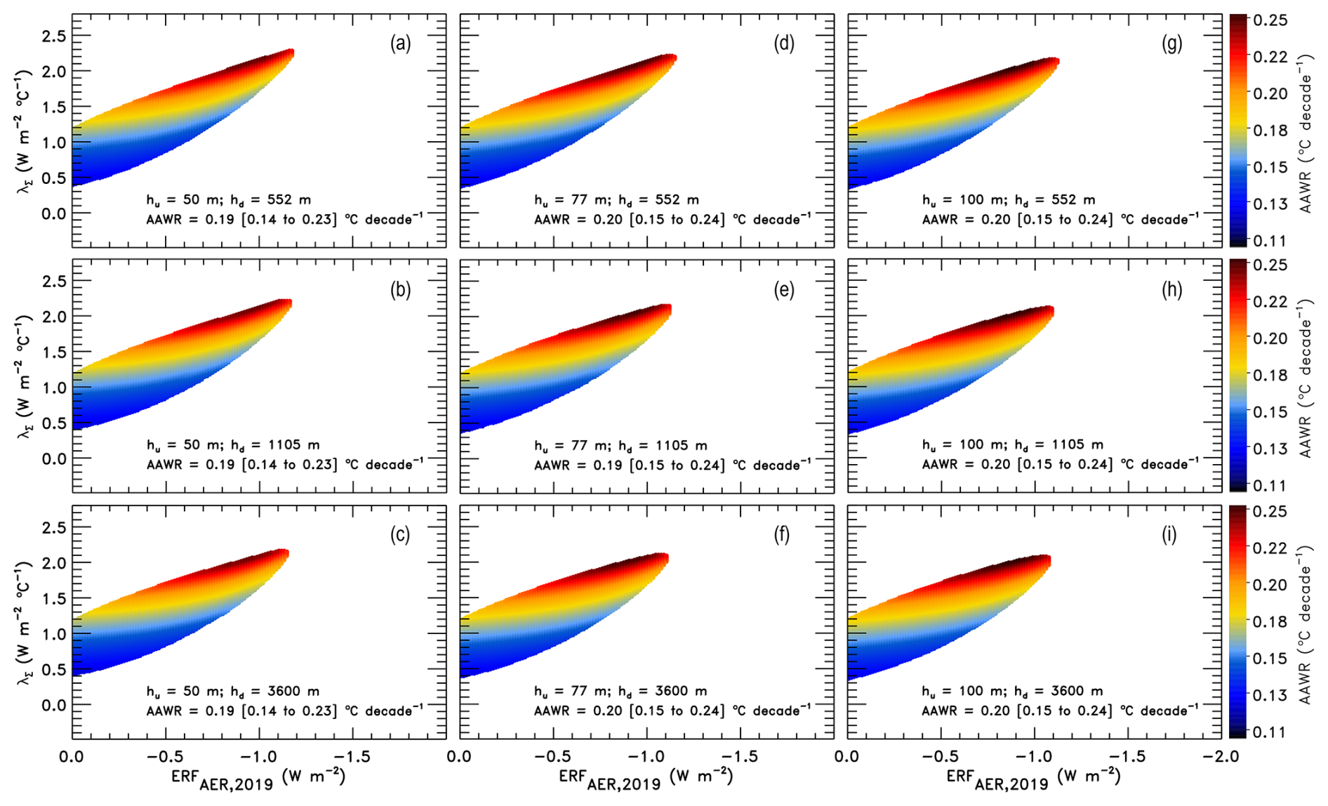
Figure A1 Values of AAWR as the function of climate feedback and ERF_AER,2019 (Sect. 2.1.2), for nine different combinations of the equivalent depth of the upper (h_u) and lower (h_d) layers of the two-layer EBM. The 50th percentile and the 5 %–95 % range of AAWR from the weighted ensemble are also given on each panel.

A3 Calibration of heat capacities

In this section, we describe the setup of the effective heat capacities of the upper and lower layers of the two-layer EBM, termed C_u and C_d, respectively. C_u and C_d are expressed per unit area of the ocean, and have the dimensions of J m⁻² K⁻¹. Geoffroy et al. (2013a) and Geoffroy et al. (2013b) calibrated the two-layer EBM using the output of abrupt4xCO₂ simulations from a set of CMIP5 models. Geoffroy et al. (2013b) found the values of C_u=7.3 $\mathrm{W}\mathrm{yr}{\mathrm{m}}^{-\mathrm{2}}{\mathrm{K}}^{-\mathrm{1}}$ and C_d=106 $\mathrm{W}\mathrm{yr}{\mathrm{m}}^{-\mathrm{2}}{\mathrm{K}}^{-\mathrm{1}}$ based on the CMIP5 multi-model mean, which correspond to equivalent depths of 77 and 1105 m. For the simulations presented in this paper, we use the same equivalent depths for the two layers within our model.

An important consideration for the implementation of EBM–1 within the EM–GC is the model's sensitivity to the heat capacities of the two layers. Therefore, we performed a set of simulations to test the sensitivity of our model output to the values of C_u and C_d. We tested three values of C_u (4.8, 7.3 and 9.6 $\mathrm{W}\mathrm{yr}{\mathrm{m}}^{-\mathrm{2}}{\mathrm{K}}^{-\mathrm{1}}$), combined with three values of C_d (53, 106 and 344 $\mathrm{W}\mathrm{yr}{\mathrm{m}}^{-\mathrm{2}}{\mathrm{K}}^{-\mathrm{1}}$), for a total of nine simulations. The equivalent depths that correspond to these heat capacities are 50, 77 and 100 m for the upper layer, and 552, 1105 and 3600 m for the lower layer. These values were picked to represent a wide range of heat capacities, and to include pairings where the ratio of C_u to C_d is similar to that inferred from CMIP5/6 simulations.

Figure A1 shows the values of AAWR for the λ_Σ–ERF_AER ensemble across the nine benchmark simulations, in a manner similar to Fig. 2. The nine panels in Fig. A1 correspond to the nine combinations of equivalent depths for the two layers, as indicated in the individual panels. Similarly to Fig. 2, the colored regions in Fig. A1 correspond to values of AAWR as indicated by the color bars to the right, for combinations of λ_Σ and ERF_AER,2019 that satisfy all three reduced χ² constraints. We also provide computed values of the effective climate sensitivity (EffCS) and the parameter γ for the nine benchmark simulations in a similar manner in Figs. S4 and S5, respectively.

Across the nine simulations, we find that the values of EffCS are generally consistent, while the range of AAWR is virtually identical. Therefore, while the estimated range of γ changes considerably depending on the heat capacities of the upper and the lower layers (Fig. S5), the regression to the historical GMST and OHC record is largely unaffected (Figs. A1 and S4). Finally, we performed simulations of the IMO–0.1 scenario (Sect. 2.2.2) for all nine benchmark depth combinations. We find a negligible difference in the impact of IMO2020 on the modelled GMST across the nine depth combinations. Consequently, the results presented in this paper are largely unaffected by the specific values of C_u and C_d.

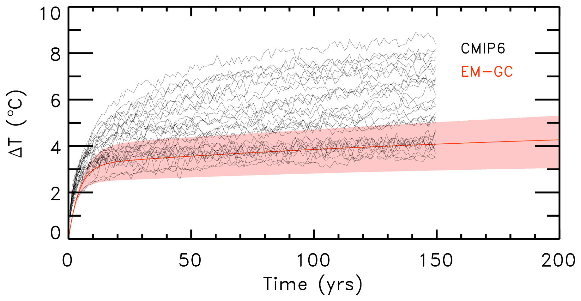
Figure A2 Modelled GMST during an abrupt4xCO₂ simulation performed with the updated EBM module of EM–GC (red). The solid line and the shading correspond to the 50th percentile, and the 5 %–95 % range, respectively. The black lines represent abrupt4xCO₂ simulations from an ensemble of 28 CMIP6 models as described in McBride et al. (2021).

The abrupt4xCO₂ experiment was performed with the EM–GC EBM module using the same equivalent depths for the two layers (77 and 1105 m for the upper and lower layers, respectively) as for the simulations described in the main paper. Figure A2 shows the time evolution of the GMST under abrupt4xCO₂ conditions projected by EM–GC (red), and by an ensemble of 28 CMIP6 models from McBride et al. (2021). McBride et al. (2021) found that eight members of this CMIP6 ensemble produces EffCS and AAWR consistent with EM–GC estimates, using an earlier version of EM–GC. These eight CMIP6 models are listed in Fig. S17 of McBride et al. (2021). There are nine CMIP6 models in Fig. A2 that produce a temperature response that are within the range simulated by EM–GC: GFDL–ESM4; GISS–E2–1–G; GISS–E2–2–G; INM–CM4–8; INM–CM5–0; MIROC6; MIROC–ES2L; NorESM2–LM; NorESM2–MM. Eight of these models are the same as the ones in Fig. S17 of McBride et al. (2021). In addition to these eight models, the temperature response of the GISS–E2–2–G model was also found to be consistent with EM–GC in Fig. A2.