A risk assessment framework for interacting tipping elements

Tipping elements, such as the Greenland Ice Sheet, the Atlantic Meridional Overturning Circulation (AMOC) or the Amazon rainforest, interact with one another and with other non-linear systems such as the El Niño-Southern Oscillation (ENSO). In doing so, the risk of any one element being degraded can be drastically affected, typically increasing due to the interactions. Therefore, in this work we propose a fully probabilistic network model for risk assessment of interacting tipping elements that coherently incorporates literature-based expert assessments of inter-element interactions. For fixed levels of global warming, we provide analytic results for the risk of being degraded for 8 interacting tipping elements and ENSO at equilibrium, including the stability of and convergence times to this equilibrium solution. Moreover we simulate their tipping risks until 2350 using emission pathways from the Shared Socio-economic Pathways (SSP 1-1.9, 1-2.6, 2-4.5, 3-7.0, and 5-8.5). Compared to the interaction-free baseline, we find that interactions tend to destabilise the climate system. For instance the coral reefs are likely to have collapsed by 2100 even under the most optimistic scenario (SSP1-1.9). The effects of interactions, however, are most noticeable after 2100, especially for the SSP scenarios with the strongest greenhouse gas emissions (SSP3-7.0 and SSP5-8.5). In summary, our risk assessment framework for tipping elements and ENSO indicates that rapid mitigation is essential to keep temperatures as close as possible to 1.5 °C in the short term and below 1 °C in the longer run.

1 Introduction

The dynamics of Earth systems often show non-linearity such as threshold effects in temperature (Burke et al., 2018; Westerhold et al., 2020). The West Antarctic Ice Sheet (WAIS), for example, is a global climate tipping element (TE) (Armstrong McKay et al., 2022) which may undergo a self-sustaining collapse due to marine ice sheet instability (Feldmann and Levermann, 2015; Waibel et al., 2018) should it pass its tipping point. More generally, tipping elements are subsystems of a larger system, for example the climate, that may pass a tipping point (Lenton et al., 2008). Merely observing and assessing the state of one can be a challenging endeavour – WAIS evolves over hundreds to thousands of years (Van Breedam et al., 2020; Armstrong McKay et al., 2022) and there is often insufficient data to cover the entirety of its life cycle. Moreover, to understand one tipping element is to grasp its many components across a hierarchy of scales, using various perspectives and often inter-disciplinary approaches (Wimsatt, 1994).

Furthermore, tipping points are not independent of each other; they can stabilise and destabilise other ones, causing cascading effects that propagate throughout the entire Earth system (Rocha et al., 2018; Steffen et al., 2018; Wunderling et al., 2024). In general, most interactions between tipping elements are destabilizing, increasing the likelihood of tipping cascades, wherein one element tipping causes others to tip, potentially cascading through the Earth system as a whole (Wunderling et al., 2023, 2024). Even at the local or regional levels, interacting ecological regime shifts can undergo similar tipping cascades (Rocha et al., 2018). However, there are some notable exceptions, namely involving AMOC. For example, Sinet et al. (2025) found that WAIS may stabilise the Atlantic Meridional Overturning Circulation (AMOC) through meltwater flux contingent upon the rates of and delays between their collapse. Jackson et al. (2015) found that a weakening AMOC may cause intense cooling of the Greenland ice sheet. Moreover, the reduction in northward heat transport following the AMOC weakening was found to stabilise Arctic sea ice (Liu and Fedorov, 2022).

In the literature on interacting tipping elements, the frequently cited seminal work by Kriegler et al. (2009) is an expert elicitation seeking to characterise/quantify the individual tipping points as well as to bound the conditional probability – what the authors call a probability ratio or PF – of one element being triggered given that another has already tipped. For example, after systematic weighting, the experts judged that if WAIS has already deteriorated, then the probability for the Greenland Ice Sheet (GIS) to trigger increases by a factor of 1 to 2. This systematic elicitation has then informed several of the past tipping point assessments (Wunderling et al., 2021a); in qualitative Boolean models (Gaucherel and Moron, 2017); in a conceptual mechanistic model (Sinet et al., 2023); and in dynamical systems models (Cai et al., 2016; Wunderling et al., 2020, 2021a, 2023) where it often has informed model calibration and parametrisation of interactions.

These modelling approaches, however, are limited regarding their treatment of uncertainty. First, uncertainty has only been studied either through stochastic noise or through sampling parameter values from confidence intervals. An important phenomenon resulting from the former is noise-induced tipping (N-tipping) where fluctuations push a system outside of a basin of attraction (Ashwin et al., 2012). The latter, meanwhile, is often accounted for via computationally heavy Monte Carlo simulations such as in Wunderling et al. (2021a), Wunderling et al. (2021b), Wunderling et al. (2023), Rosser et al. (2024). Second, although other works have modelled individual tipping elements (TEs) probabilistically (Barfuss et al., 2018, 2020) they neglect the interactions between tipping elements which may cause a cascade of tipping events. Third, even in dynamical models that do consider the TE-TE interactions (Wunderling et al., 2020, 2021a, b, 2023), these were implemented as linearly additive coupling terms in the evolution of some state variable or observable, whereas the pairwise PFs of Kriegler et al. (2009) are multiplicative factors that act on the probability of a TE being tipped, not on some state variable.

We remedy some of these shortcomings by providing a risk assessment modelling framework of interacting tipping elements with a more coherent treatment of uncertainty, which is also computationally more efficient. We take the perspective that the environment itself is probabilistic insofar as the “real” state of the system is indirectly measured/observed, due to its complex nature and even its conceptualisation. We thus model each tipping element as a 2-state Markov chain with a Prosperous state and a Degraded state, similarly to other probabilistic approaches (Barfuss et al., 2018, 2020, 2024), whose transitions, in contrast to those previous models, further depend on the state of their network neighbours. In this way, though there is a latent state for each tipping element to be in, what is modelled/observed is the probability to be in, say, the Degraded state. This allows us to greatly reduce the dimensions of the Monte Carlo ensembles requiring, therefore, far less heavy computation.

Moreover, our approach inherently allows for conditional interactions, that is the probability for one tipping element to be triggered is increased/decreased when another has tipped, more coherently incorporating the probability factors derived through expert elicitation (Kriegler et al., 2009), unlike the linearly additive interaction terms in other models (Wunderling et al., 2020, 2021a, b, 2023). Finally, by taking a probabilistic approach, we soften their assumption that “a state change is initiated as soon as the increase in GMT exceeds the critical temperature” (Wunderling et al., 2021a). We do so by introducing a tipping “belief” which is a logistic function in global warming, parametrised by the likely estimates and bounds on the critical temperature threshold for each element (Armstrong McKay et al., 2022). In effect, even though there is uncertainty with regards to the exact value of the critical threshold, the higher the global warming level is above the minimum threshold estimate, the more likely we believe each element is to begin to tip. Furthermore, through this temperature dependence we incorporate the anthropogenic drivers and effects on environmental dynamics, which are mediated by global warming, using the SSP scenarios from the IPCC's Sixth Assessment Report (Lee et al., 2021) for analysis of the short-term risk and a range of fixed levels for the equilibrium risk.

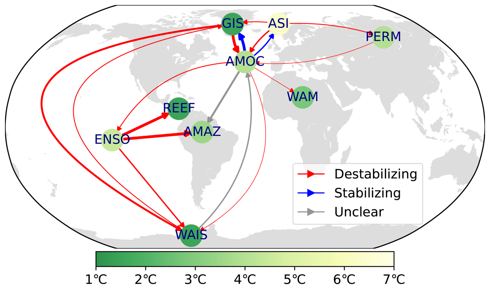
Figure 1 Illustration of the tipping element interaction network, with data from Armstrong McKay et al. (2022) and Wunderling et al. (2024). Nodes represent individual tipping elements with their colours indicating the mean of the respective tipping threshold temperature. Node locations are not exhaustively representative but have instead been chosen for illustrative purposes; for example, low-latitude coral reefs are also found around the islands of Indonesia and off the east coast of Africa. Moreover, note that, although its status as a tipping element is debated (Armstrong McKay et al., 2022), we include the El Niño-Southern Oscillation (ENSO) due to its important feedbacks on both global core and regional tipping elements. Edges indicate interactions due to one tipping element on another, with destabilizing edges in red, stabilizing in blue, and unclear/mixed in gray. Edge thickness indicates the maximum value of the signed edge weight, thus thicker edges denote potentially stronger interactions.

In Sect. 2 we introduce our probabilistic approach to modelling interacting tipping elements: first, we set up the mathematical framework for a network of interacting Markov chains (Sects. 2.1 and 2.2) and including effects due to global warming (Sect. 2.3); second, in Sect. 2.4 we give an overview of the 8 tipping elements and the El Niño-Southern Oscillation (ENSO) including their inferred parameters and their pairwise interactions which is further illustrated in Fig 1. Having established the model and parametrisation thereof, in Sect. 3.1 we present the theoretical analysis regarding the degradation risk at equilibrium (Sect. 3.1.1), their stability (Sect. 3.1.2) and the convergence time of long-term solutions to the equilibrium (Sect. 3.1.3). Using numerical methods (see Appendix B1), we evaluate the equilibrium solution for the interacting network of tipping elements and ENSO in Sect. 3.2 and provide computational simulation results (for detail on computational methods, see Appendix B2) for their short-term evolution under various extended SSP scenarios in Sect. 3.3. We conclude with a discussion of our results in Sect. 4.

2 Methods

In this work, we model our tipping elements and ENSO each as a 2-state Markov chain, which can either be prosperous or degraded. Therefore we first introduce the mathematical preliminaries for any general 2-state Markov chain including their dynamics and any steady state solutions in Sect. 2.1. Note that to model a dynamical system as a Markov chain does not inherently require nor necessarily imply that the system displays any irreversibility nor self-perpetuation thresholds. In other words a Markov chain can model systems which do not contain tipping points, such as ENSO.

We then go beyond individual independently evolving Markov chains in Sect. 2.2 by extending the model to a network of coupled Markov chains, embodying the tipping interactions that occur between tipping elements and ENSO. For example when one Markov chain is in the degraded state this can either increase or decrease the collapse transition of a different Markov chain. In Sect. 2.3 we discuss how tipping timescales are re-interpreted as the transition rates of a Markov chain while also including the effects of temperature on tipping. Finally we discuss the parametrisation of our model using data from previous tipping element reviews, namely those of Armstrong McKay et al. (2022) for individual element data and Wunderling et al. (2024) for the interactions.

2.1 Two-State Markov chains preliminary

In general, a 2-state Markov chain (MC) is characterised by its two possible states S₀ and S₁ with two transition probabilities p and q. In particular, p is the probability to to go from state S₀ to S₁ in one time-step while similarly q is the probability from S₁ to S₀. This is summarised by the transition matrix $\mathbf{T}=(T_{S{S}^{\prime }}:S,S^{\prime }\in \mathit{\{}{S}_{\mathrm{0}},S_{\mathrm{1}}\mathit{\left\}}\right)$ given in Eq. (1).

$$\begin{array}{}\text{(1)}& \mathbf{T}=\left(\begin{array}{cc}\mathrm{1}-p& p\\ q& \mathrm{1}-q\end{array}\right)\end{array}$$

The update equation for the probability to be in one of the states, say state S₁, at time t+1, ℙ_t+1(S₁), can then be found in terms of p,q and the probability at the previous time-step t, ℙ_t(S₁), given by Eq. (2).

$$\begin{array}{}\text{(2)}& {\mathbb{P}}_{t+\mathrm{1}}\left(S_{\mathrm{1}}\right)=p(\mathrm{1}-{\mathbb{P}}_t(S_{\mathrm{1}}\left)\right)+(\mathrm{1}-q){\mathbb{P}}_t\left(S_{\mathrm{1}}\right)\end{array}$$

The dynamics of the whole chain are fully captured by the dynamics of one state since we have $\mathbb{P}\left(S_{\mathrm{0}}\right)+\mathbb{P}\left(S_{\mathrm{1}}\right)\equiv \mathrm{1}$. Given an initial distribution of ℙ₀(S₁) at time t=0, the explicit time evolution at time t is given by Eq. (3).

$$\begin{array}{}\text{(3)}& {\mathbb{P}}_t\left(S_{\mathrm{1}}\right)={\displaystyle \frac{p}{p+q}}(\mathrm{1}-(\mathrm{1}-p-q{)}^{t-\mathrm{1}})+(\mathrm{1}-p-q{)}^t{\mathbb{P}}_{\mathrm{0}}\left(S_{\mathrm{1}}\right)\end{array}$$

At equilibrium, ${\mathbb{P}}_{t+\mathrm{1}}\left(S_{\mathrm{1}}\right)={\mathbb{P}}_t\left(S_{\mathrm{1}}\right)$, giving the stationary distribution, ℙ_∗(S₁), in Eq. (4) which, assuming fixed p,q, is stable if $p+q>\mathrm{0}$.

$$\begin{array}{}\text{(4)}& {\mathbb{P}}_{\ast }\left(S_{\mathrm{1}}\right)={\displaystyle \frac{p}{p+q}}\end{array}$$

To find the stability of the stationary distribution in Eq. (4) corresponds to finding the eigenvalues of the Jacobian matrix at the stationary distribution, which, in this case, is simply the derivative of Eq. (2). Formally, for x=ℙ_t(S₁) and a map $f:[\mathrm{0},\mathrm{1}]\to [\mathrm{0},\mathrm{1}]$ such that ${\mathbb{P}}_{t+\mathrm{1}}\left(S_{\mathrm{1}}\right)=f\left(x\right)$, the stationary distribution $x_{\ast }={\mathbb{P}}_{\ast }\left(S_{\mathrm{1}}\right)$ is stable if $\left|f^{\prime }\right(x_{\ast }\left)\right|<\mathrm{1}$. From Eq. (2), $f^{\prime }\left(x\right)=\mathrm{1}-(p+q)$ such that the stability condition simply becomes $\mathrm{0}<p+q<\mathrm{2}$.

2.2 Interacting Markov chains

For a set of Markov chains, V, let $G=\mathit{\{}V,E\mathit{\}}$ be a graph of pairwise interactions between individual Markov chains. A directed edge $(i,j)\in E$ exists if there is a causal link or effect due to MC i∈V on another MC j∈V, disallowing self-loops. An element a_ij of the adjacency matrix $\mathbf{A}=(a_{ij}:\forall i,j\in V)$ corresponds to the probability factor PF(i→j) due to one tipping element i being triggered on another element j. In general the edge from i to j is represented by a_ij which may be weighted – indicating some positively valued coupling strength – and signed – indicating the polarity of the effect (e.g. stabilising or destabilising). For signed edges, we denote the adjacency matrix of destabilising edges with ${\mathbf{A}}^{+}=(a_{ij}^{+}:\forall i,j\in V)$ with with $a_{ij}^{+}=\mathrm{PF}(i\to j)$ when $\mathrm{PF}(i\to j)>\mathrm{1}$. Similarly, we denote ${\mathbf{A}}^{-}=(a_{ij}^{-}:\forall i,j\in V)$ all the stabilising edges, i.e. those with $\mathrm{PF}(i\to j)<\mathrm{1}$ has a corresponding adjacency element $a_{ij}^{-}=\mathrm{PF}(i\to j{)}^{-\mathrm{1}}$.

The state of each MC i∈V is denoted by 𝒮_i which can take one of two environmental states – either Prosperous 𝒫 or Degraded 𝒟 – and has an associated internal collapse probability $p_{\mathrm{c},i}\in (\mathrm{0},\mathrm{1})$ and recovery probability $p_{\mathrm{r},i}\in (\mathrm{0},\mathrm{1})$, which are the Markov transition probabilities between the possible environmental states due to the internal processes alone. Moreover, let the probability of node i being in the Degraded state be denoted $D_i\equiv \mathbb{P}({\mathcal{S}}_i=\mathcal{D})$. As probability factors are conditional upon one element having already been triggered, then, in general, degraded destabilising in-neighbours increase the collapse probability, while stabilising ones decrease the probability to collapse. We therefore modify the individual collapse probability by the interactions due to all in-neighbours into an effective probability to collapse ${\stackrel{\mathrm{̃}}{p}}_{\mathrm{c},i}$.

$$\begin{array}{}\text{(5)}& {\stackrel{\mathrm{̃}}{p}}_{\mathrm{c},i}=p_{\mathrm{c},i}{\displaystyle \frac{\mathrm{1}+{\sum }_{j\in V}{a}_{ji}^{+}{D}_j}{\mathrm{1}+{\sum }_{j\in V}{a}_{ji}^{-}{D}_j}}\end{array}$$

Each Markov chain evolves according to the transition matrix in Eq. (1) and the corresponding update equation in Eq. (2) with $p={\stackrel{\mathrm{̃}}{p}}_{\mathrm{c},i}$ and $q=p_{\mathrm{r},i}$, however there is now a dependence on the states of its in-neighbours. As such an explicit expression for the time evolution of each node requires solving a set of non-linear coupled maps, such that a general solution is cumbersome to write down as a closed form expression. Instead, as in Eq. (2), we derive the update equation D_i[t+1] in Eq. (6). Note for notational brevity, where relevant, all terms in the right hand side of the equation are evaluated at time t.

$$\begin{array}{}\text{(6)}& D_i[t+\mathrm{1}]={\displaystyle \frac{\mathrm{1}+{\sum }_{j\in V}{a}_{ji}^{+}{D}_j}{\mathrm{1}+{\sum }_{j\in V}{a}_{ji}^{-}{D}_j}}{p}_{\mathrm{c},i}(\mathrm{1}-D_i)+(\mathrm{1}-p_{\mathrm{r},i})D_i\end{array}$$

2.3 Anthropogenic collapse and recovery

Moving away from the abstract, in this subsection, we address the question of how long a time-step is and make explicit the one-to-one correspondence between probabilities and tipping timescales. We then introduce how global warming temperatures, as a proxy of human impact, change the transition probabilities.

First, consider that the update equations describing the dynamics of a Markov chain generally, e.g. in Eq. (2). There they describe how the probability to be in one state S₁ at the next model time-step t+1 depends on the probability at the current time-step t. In other words, the Markov chain evolves over discrete and dimensionless time-steps. In order to translate such model time-steps into physical units of time, we set the duration of a time-step to be τ_m years. In principle τ_m could be any value and represents the temporal precision of the model. However note, as we will see in Sect. 3.1.2, that the discretisation of time can influence ergodicity and therefore stability of the stationary distribution.

We now make the correspondence between tipping timescales and probabilities. Consider the transition from one state to another, which on average is expected to take τ amounts of real time, say τ years to be concrete. Then, given some duration of time τ_m, the effective probability for the state transition to occur within that time-frame τ_m, conditional upon having been triggered, is given by $p=(\mathit{\tau }/{\mathit{\tau }}_{\mathrm{m}}+\mathrm{1}{)}^{-\mathrm{1}}$. Here, the plus one is to ensure that if τ=0 then certainly, i.e. with p=1, the transition has occurred within τ_m. With regards to tipping elements, once an element i has crossed its threshold, it does not instantly transition to its new state, rather it collapses over some timescale τ_c,i. Similarly, we can construct a recovery transition probability p_r,i given a subsystem's recovery timescale.

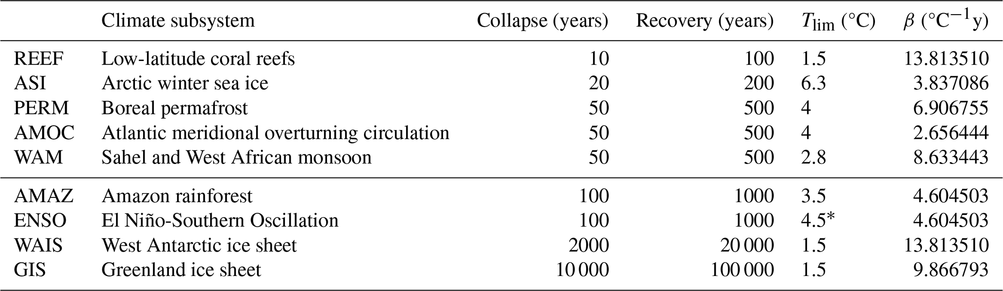
Table 1 Summary table of tipping elements and ENSO and their respective parameters (τ_c,i, τ_r,i, T_lim,i, β_i) as inferred from the literature review of Armstrong McKay et al. (2022). Given the lack of knowledge regarding specific numerical values for the recovery timescales, we assume all recovery times are at least an order of magnitude larger than their respective collapse times, i.e. ${\mathit{\tau }}_{\mathrm{r},i}=\mathrm{10}{\mathit{\tau }}_{\mathrm{c},i}$ $\forall i\in V$ where V is the set of climate subsystems – in doing so we also respect the (ir)reversibility of the tipping elements summarised by the Global Tipping Points Report 2023 (Lenton et al., 2023). ^∗ ENSO threshold was estimated as the midpoint of the range given in the Supplementary Data S1 of Armstrong McKay et al. (2022).

The dynamics of nature are not purely driven by natural/physical processes but also by the actions of individuals, stakeholders and institutions. Although there are many anthropogenic drivers of environmental/ecological collapse, some of which are not directly correlated with global warming (e.g. deforestation for agricultural land), we consider all anthropogenic effects as being mediated by – or at the very least proxied/dominated by – global warming. That is, as Armstrong McKay et al. (2022) finds, when the global mean surface temperature (GMST) exceeds the critical threshold of an individual tipping element, that element is far more likely to be triggered and thus begin its timely collapse. To that end, for each tipping element or ENSO, i, we do a similar decomposition into the likelihood to be triggered (which is a function of global warming) multiplied by the conditional probability of tipping discussed previously $({\mathit{\tau }}_{\mathrm{c},i}/{\mathit{\tau }}_{\mathrm{m}}+\mathrm{1}{)}^{-\mathrm{1}}$. In particular, given a GMST anomaly relative to pre-industrial times of ΔT, for element i with timescales τ_c,i and τ_r,i and an estimated critical temperature threshold of T_lim,i we have that the internal probabilities to recover and collapse are given by,

$$\begin{array}{}\text{(7)}& \begin{array}{rl}& p_{\mathrm{r},i}={\displaystyle \frac{\mathrm{1}}{({\mathit{\tau }}_{\mathrm{r},i}/{\mathit{\tau }}_{\mathrm{m}})+\mathrm{1}}},\\ & p_{\mathrm{c},i}={\displaystyle \frac{\mathrm{1}}{({\mathit{\tau }}_{\mathrm{c},i}/{\mathit{\tau }}_{\mathrm{m}})+\mathrm{1}}}\cdot {\displaystyle \frac{\mathrm{1}}{\mathrm{1}+\exp (-{\mathit{\beta }}_i(\mathrm{\Delta }T-T_{\text{lim},i}\left)\right)}}\end{array}\end{array}$$

where τ_m is the duration of a model time-step in units of years – unless otherwise stated we henceforth set τ_m=1 year – and β_i is the sensitivity of the logistic function.

One way to interpret this parameter is physically: if a tipping point with low β_i has crossed its threshold by a small amount then its tipping probability is only marginally increased; whereas one with a high β_i would experience a large increase in its tipping probability. Another way, as we do in this work, is to quantify the deep uncertainty amongst the expert assessments: that is when the range of plausible tipping thresholds is large, indicating the wide range in expert opinion, the sensitivity β_i is low; whereas a small range in the threshold suggests a high degree of confidence and/or agreement and therefore a high β_i. For details on how we infer the value of β_i see Appendix A1.

2.4 Tipping elements of the Earth system

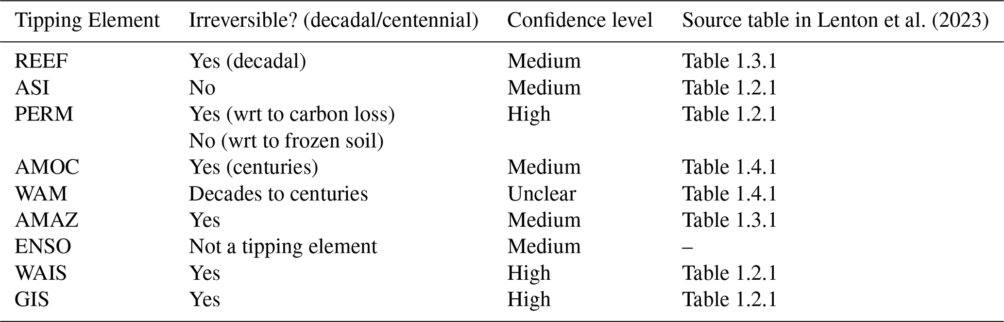
Armstrong McKay et al. (2022) comprehensively assessed 16 tipping, through their extensive multi-disciplinary literature review, providing estimates on, amongst others, the tipping threshold and timescales. In total the authors had reviewed 33 possible tipping elements, however in our work, due to the limited amount of TE-TE interaction data available (Wunderling et al., 2024), we focus only on nine of them – 6 global core tipping elements, two regional elements (low-latitude coral reefs and the Sahel and West African monsoon) and the El Niño-Southern Oscillation (ENSO) whose status as a tipping element has been disputed (Collins et al., 2019; Lee et al., 2021). As our model is agnostic to the precise definition of a tipping element – for example as one containing hysteresis or irreversibility – and regardless of its classification, we include ENSO in our case study since it has direct, strongly destabilising impacts on other subsystems, notably on the coral reefs and on the Amazon rainforest (Wunderling et al., 2024). ENSO's “collapse” transition can be thought of as the shift towards a state of increased El Niño amplitude (Lenton et al., 2008) and/or increased rainfall amplitude variability (Armstrong McKay et al., 2022). Table 1 summarises for each tipping element and ENSO the set of parameters inferred from the review, namely the timescales for collapse and recovery, the tipping threshold and the sensitivity to temperature. For specific timescale values and inference methods, especially for the sensitivity, see Appendix A1.

For the interactions between tipping elements we rely on a similarly extensive literature review by Wunderling et al. (2024), in which the authors had assessed four properties of 19 pairwise interactions: response type, response strength, level of agreement within the literature and level of evidence. Although the review described response strengths in qualitative terms, a core foundation of the review comes from the quantitative probability factors of the expert elicitation (Kriegler et al., 2009). We use a similar methodology from an earlier work (Wunderling et al., 2021a) to, first, convert the qualitative terms back into probability factors, thus allowing us to include the new interactions considered. For specifics, see Appendix A2.

A major challenge here is the deep uncertainty within the literature where interactions are concerned (Lam and Majszak, 2022; Wunderling et al., 2024). That is, in some cases, there is not even general consensus as to whether a particular interaction is destabilising or stabilising. For example, there are multiple opposing mechanisms which allow the West Antarctic ice sheet to either strengthen (Pedro et al., 2018; Li et al., 2023) or weaken (Stouffer et al., 2007) AMOC, while other works suggest the disintegration of WAIS can avoid (Sinet et al., 2025) or at least delay (Sadai et al., 2020) the subsequent collapse of AMOC. Therefore, in order to reflect the uncertainty both from the original expert elicitation (Kriegler et al., 2009) and the more recent review (Wunderling et al., 2024), we associate with each pairwise interaction a uniform random distribution whose range is the interval of plausible PF values (see Fig. 1 for illustration or Table A2 for details). Note, that since a uniform random distribution maximizes entropy or uncertainty given a constrained interval, no further assumptions other than the range of plausible PF values are needed. Moreover, note that, in this work, we discard all interactions with both unclear response type and unclear response strength (in total, 2 of the original 19 interactions from Wunderling et al., 2024), as we found no clear, reasonable way to quantify such interactions. Given the 17 dimensional space of parameters, we use a Monte Carlo ensemble of simulations using the Latin hypercube sampling method (McKay et al., 1979), which covers the parameter space more efficiently than i.i.d sampling (for more computational detail see Appendix B1).

3 Results

3.1 Theoretical solutions

3.1.1 Equilibrium solutions

In this subsection, we will derive the system-wide stationary distribution of our tipping elements network. A source node s∈V, i.e. a node which has no in-neighbours, behaves precisely as an independent 2-state Markov chain with $p=p_{\mathrm{c},\mathrm{s}}$ and $q=p_{\mathrm{r},\mathrm{s}}$ as it is unaffected by any other nodes. For completion we include the update equation for D_s[t+1] below, however the explicit the time-evolution D_s(t) and stationary distribution $D_{\ast ,\mathrm{s}}$ can be derived directly from Eqs. (3) and (4) by simple substitutions.

$$\begin{array}{}\text{(8)}& {\displaystyle }\begin{array}{rl}{D}_{\mathrm{s}}\left(t\right)=& D_{\ast ,\mathrm{s}}\left(\mathrm{1}-(\mathrm{1}-p_{\mathrm{c},\mathrm{s}}-p_{\mathrm{r},\mathrm{s}}{)}^{t-\mathrm{1}}\right)\\ & +(\mathrm{1}-p_{\mathrm{c},\mathrm{s}}-p_{\mathrm{r},\mathrm{s}}{)}^t{D}_{\mathrm{s}}(\mathrm{0})\end{array}\text{(9)}& {\displaystyle }{D}_{\ast ,\mathrm{s}}={\displaystyle \frac{p_{\mathrm{c},\mathrm{s}}}{p_{\mathrm{c},\mathrm{s}}+p_{\mathrm{r},\mathrm{s}}}}\end{array}$$

Assume now there exists a stationary joint-distribution ${\mathit{D}}_{\ast }=(D_{\ast ,i}:i\in V)$ for the entire system which satisfies, for each i∈V, $D_{\ast ,i}[t+\mathrm{1}]=D_{\ast ,i}\left[t\right]$. Plugging this ansatz into the update equation in Eq. (6) results in $\left|V\right|$ simultaneous equations as seen in Eq. (10); although there is no explicit, closed-form expression the coupled equations can be solved numerically. Notice the solution for source nodes, s∈V, can also be derived from these equations directly by noting that all $a_{j,s}^{\pm }=\mathrm{0}$. Due to the logistic dependence of p_c,i on global warming ΔT, the equilibrium probability to be degraded $D_{\ast ,i}$ is also dependent on global warming. In the limit of low temperatures, all $p_{\mathrm{c},i}\to {\mathrm{0}}^{+}$ such that the equilibrium Degraded risk similarly tends to 0. As temperature increases, Eq. (10) increases monotonically until it converges to a high temperature limit $D_{\ast ,i}^{\text{hot}}$ from below, since all $p_{\mathrm{c},i}\to ({\mathit{\tau }}_{\mathrm{c},i}+\mathrm{1}{)}^{-\mathrm{1}}$ also from below.

$$\begin{array}{}\text{(10)}& D_{\ast ,i}={\displaystyle \frac{\left(\mathrm{1}+{\sum }_{j\in V}{a}_{ji}^{+}{D}_{\ast ,j}\right)p_{\mathrm{c},i}}{\begin{array}{c}\left(\mathrm{1}+{\sum }_{j\in V}{a}_{ji}^{+}{D}_{\ast ,j}\right)p_{\mathrm{c},i}\\ +\left(\mathrm{1}+{\sum }_{j\in V}{a}_{ji}^{-}{D}_{\ast ,j}\right)p_{\mathrm{r},i}\end{array}}}\end{array}$$

Notice that ΔT may in general evolve over some timescale τ_w; the Anthropocene has been characterised by, amongst others, rapidly increasing global temperatures over the 20th and 21st centuries, i.e. with τ_w≈ 200 years. If ${\mathit{\tau }}_{\mathrm{w}}>{\mathit{\tau }}_{\mathrm{c},i},{\mathit{\tau }}_{\mathrm{r},i}$ – in other words individual tipping elements evolve over a faster timescale, for example coral reefs and the Arctic winter sea ice (see Table 1) – the probabilities D will first settle on the stable steady state Eq. (10) parametrised by the forcing. On the other hand, for many other elements that evolve over multiple centuries or even millennia, for example WAIS and the Greenland Ice Sheet, the dynamics will be dominated by the relatively fast global warming. Therefore, for mixed systems, especially over finite times, computational simulations are necessary to complement the analytic results. For details on the simulations and numerical solutions, see Appendix B2.

3.1.2 Stability analysis

Having found a system-wide stationary distribution, we now derive conditions for its stability. A sufficient condition for the stability of the entire network is to require each individual MC to be stable, that is $\forall i\in V$ to meet the condition that $\mathrm{0}<{\stackrel{\mathrm{̃}}{p}}_{\mathrm{c},i}{|}_{\ast }+p_{\mathrm{r},i}<\mathrm{2}$ where ${\stackrel{\mathrm{̃}}{p}}_{\mathrm{c},i}{|}_{\ast }$ is the effective collapse probability evaluated at D_∗. Notice that since the internal recovery probability is restricted to $p_{\mathrm{r},i}\in (\mathrm{0},\mathrm{1})$ the condition simplifies to $\mathrm{0}<{\stackrel{\mathrm{̃}}{p}}_{\mathrm{c},i}{|}_{\ast }<\mathrm{1}$. We will now find bounds for the sums ${\sum }_j{a}_{ji}^{\pm }{D}_j$ in order to simplify the stability condition further. In particular since $D_i\in [\mathrm{0},\mathrm{1}]$ ∀i, then $\mathrm{0}\le {\sum }_j{a}_{ji}^{\pm }{D}_j\le {\sum }_j{a}_{ji}^{\pm }$. Because of this we can find lower and upper bounds for the fraction in Eq. (5) as the following,

$$\mathrm{0}<{\displaystyle \frac{\mathrm{1}}{\mathrm{1}+{\sum }_j{a}_{ji}^{-}}}\le {\displaystyle \frac{\mathrm{1}+{\sum }_{j\in V}{a}_{ji}^{+}{D}_{\ast ,j}}{\mathrm{1}+{\sum }_{j\in V}{a}_{ji}^{-}{D}_{\ast ,j}}}\le \mathrm{1}+\sum _j{a}_{ji}^{+}$$

where the first strict inequality is due to all probability factors being positively valued i.e. $a_{ij}^{\pm }\ge \mathrm{0}$ $\forall i,j\in V$, thus automatically fulfilling the first stability criterion, as the lower bound is strictly larger than 0.

Finally, since p_c,i is monotonically non-decreasing in temperature, we can upper bound the collapse probability by the hot temperature limit, in terms of the collapse timescale and the length of a model time step, $p_{\mathrm{c},i}\le (\mathrm{1}+{\mathit{\tau }}_{\mathrm{c},i}/{\mathit{\tau }}_{\mathrm{m}}{)}^{-\mathrm{1}}$, such that we have the following inequalities.

$$\begin{array}{rl}{\stackrel{\mathrm{̃}}{p}}_{\mathrm{c},i}{|}_{\ast }\equiv & {\displaystyle \frac{\mathrm{1}+{\sum }_{j\in V}{a}_{ji}^{+}{D}_j^{\ast }}{\mathrm{1}+{\sum }_{j\in V}{a}_{ji}^{-}{D}_j^{\ast }}}{p}_{\mathrm{c},i}\le \left(\mathrm{1}+\sum _j{a}_{ji}^{+}\right)p_{\mathrm{c},i}\\ & \le {\displaystyle \frac{\mathrm{1}+{\sum }_j{a}_{ji}^{+}}{\mathrm{1}+{\mathit{\tau }}_{\mathrm{c},i}/{\mathit{\tau }}_{\mathrm{m}}}}\end{array}$$

For the second criterion ${\stackrel{\mathrm{̃}}{p}}_{\mathrm{c},i}{|}_{\ast }<\mathrm{1}$ we can now compare the final expression above to 1 to arrive at the condition for D_∗ to be a stable stationary distribution.

$$\begin{array}{}\text{(11)}& {\mathit{D}}_{\ast }\text{ stable for }\sum _j{a}_{ji}^{+}<{\displaystyle \frac{{\mathit{\tau }}_{\mathrm{c},i}}{{\mathit{\tau }}_{\mathrm{m}}}}\forall i\in V\end{array}$$

Although both probability factors $a_{ji}^{+}$ and collapse timescales τ_c,i are determined from the physical system, the model time step τ_m is a free parameter, independent of the real world system. The above stability condition can therefore be used to give an upper bound for the length of the model time steps such that the equilibrium solution Eq. (10) is always stable; in other words so long as the model time step is at most ${\mathit{\tau }}_{\mathrm{m}}<{min}_{i\in V}({\mathit{\tau }}_{\mathrm{c},i}/{\sum }_j{a}_{ji}^{+})$, we can guarantee the stationary distribution is stable. Note that with our parameters this minimum occurs for the coral reefs and by setting τ_m = 1 year, our network of interacting tipping points can almost surely (i.e. with probability 1) satisfy the stability condition.

3.1.3 Convergence times

Having satisfied the stability condition, we now consider the time taken for the system to converge towards the equilibrium solution. In particular let t_ϵ be the first time step at which the probability to be degraded D(t) gets ϵ close to the equilibrium solution D_∗, in other words $\left|D\right(t_{\mathit{ϵ}})-D_{\ast }|=\mathit{ϵ}\ll \mathrm{1}$. We can approximate the evolution of the entire system by that of a single source node with collapse time τ (evolving under Eq. 8) and recovery time 10τ – given our parametrisation assumptions (see Table 1 for details) – where τ is the largest collapse time in the whole network. In so doing we can find an approximate expression (for the full derivation see Appendix C1) for t_ϵ in terms of this maximal collapse time.

$$\begin{array}{}\text{(12)}& t_{\mathit{ϵ}}\approx {\displaystyle \frac{\mathrm{10}}{\mathrm{11}}}\mathit{\tau }\ln {\mathit{ϵ}}^{-\mathrm{1}}+O\left(\mathrm{1}\right)\end{array}$$

For our network of tipping elements, for a threshold of $\mathit{ϵ}={\mathrm{10}}^{-\mathrm{3}}$ this convergence time is approximately t_ϵ≈ 63 kyr. In other words over millennial timescales, the long term behaviour of our system of 9 tipping points falls nears roughly 0.1 % (in risk percentage) of the equilibrium solution. Thus in this work any mention of “long-term” refers to millennial timescales at least.

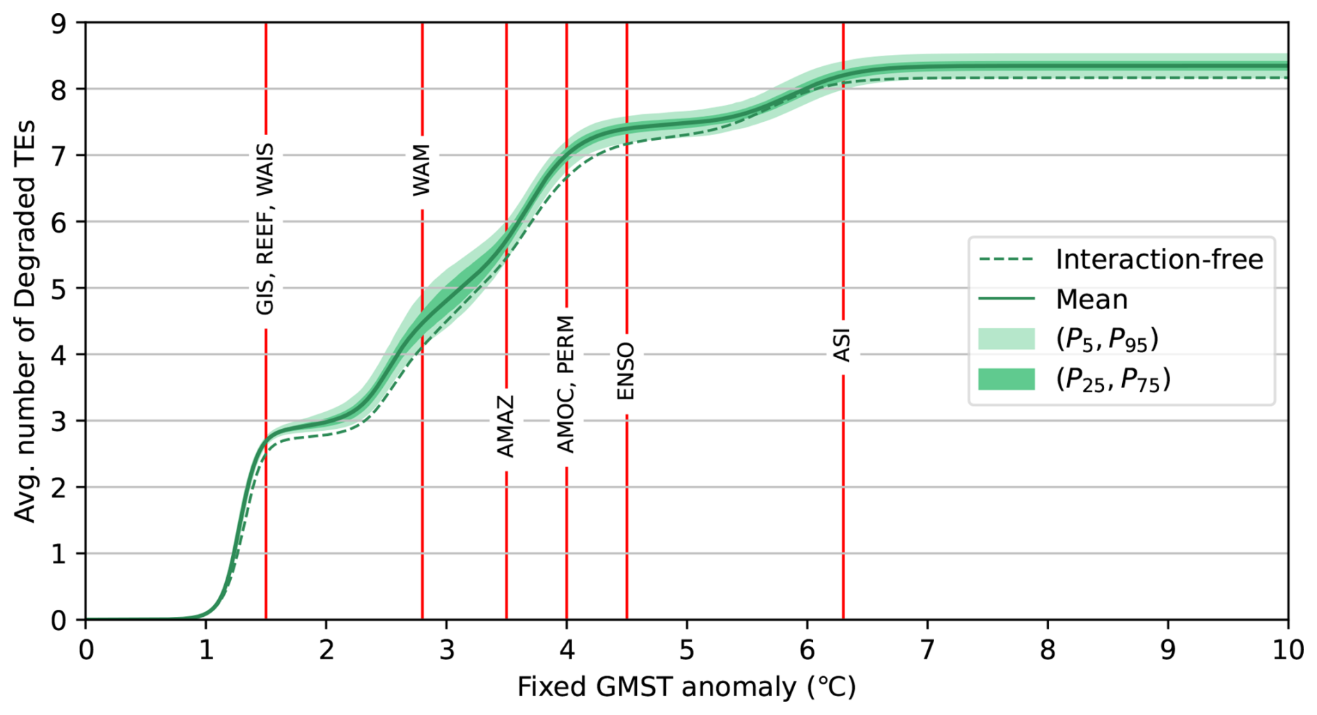
Figure 2 Expected number of degraded tipping elements at equilibrium, under a range of fixed levels of GMST anomaly. Specifically, for each value of fixed GMST anomaly, the expected number is simply the sum over all tipping elements' and ENSO's risks to be degraded, with statistics done over the ensemble of 500 interaction matrices. The dashed line indicates the interaction-free case; bold lines the ensemble mean values; while the coloured bands shows values the 5- to 95-percentile uncertainty range in lighter hue, and the first- to third-quartile uncertainty range in darker hue; vertical red lines indicate the individual critical thresholds of different tipping elements.

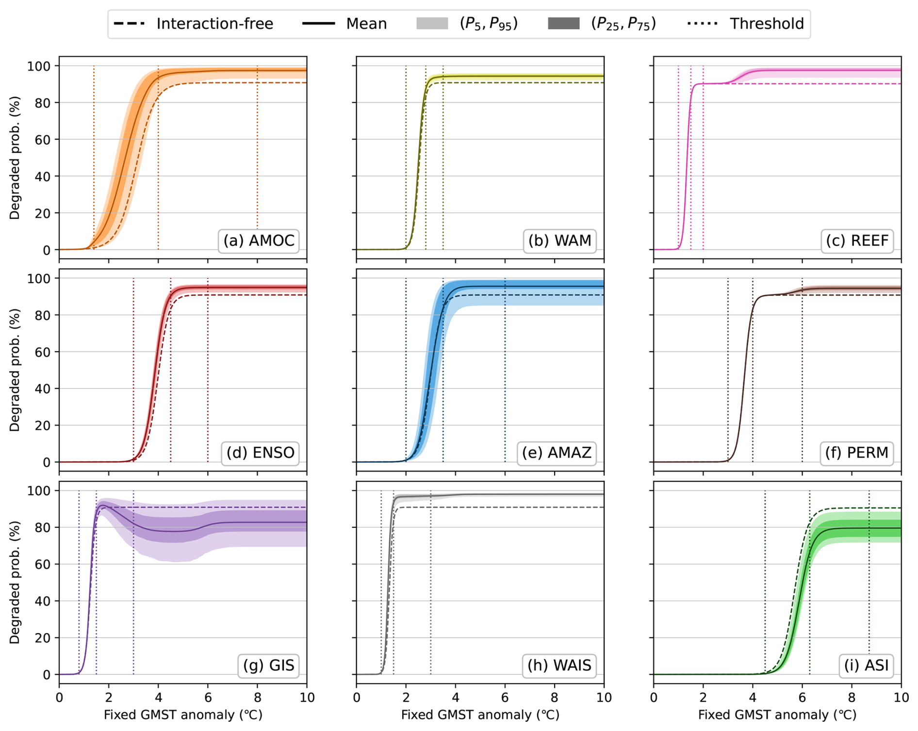
Figure 3 The stationary probability to be Degraded (see Eq. 10) of each tipping element and ENSO, for a range of fixed GMST anomaly values from +0 to +10 °C. Dashed lines indicate the interaction-free case; bold lines the ensemble mean values; while the coloured bands showing values the 5- to 95-percentile uncertainty range in lighter hue, and the first- to third-quartile uncertainty range in darker hue. The thin dotted lines indicate the tipping threshold of each element (see Table 1).

3.2 Equilibrium risks under fixed global warming levels

The stable stationary distribution of Eq. (10) can give us valuable insights into the effects of interactions – following the logic of probability factors (Kriegler et al., 2009) – on the nine climate subsystems. In particular, as the distribution is always stable, this distribution is precisely the long-term risk, after millennial times, of each tipping element being Degraded. In this subsection, we explore this equilibrium or long-term behaviour for a range of fixed GMST anomalies in terms of the expected number of degraded tipping elements (Fig. 2) and the individual risk (Fig. 3). In the former, we see that the equilibrium response of tipping elements to the global warming level is highly non-linear, due in large part to the sigmoidal temperature-dependence of each element's internal collapse probability. If we were to permanently (i.e. at least over millennial timescales) commit to the Paris Agreement global warming levels of 1.5–2 °C, then 3 tipping elements – both polar ice sheets and the low-latitude coral reefs – are very likely (> 90 %) to be in their respective degraded states as their individual critical thresholds have been surpassed.

Interactions between tipping elements on the whole increase the risk of being degraded, as indicated by the no-interactions case (dashed lines) generally lying below the ensemble mean for the with-interactions case. This is largely due to the majority of TE-TE interactions being destabilising (Wunderling et al., 2024); for some tipping elements, in fact, all of their known incoming interactions are destabilising (see Table A2) such that interactions can only ever increase stationary risks. AMOC, although mostly dominated by its destabilising neighbours, has a moderately strong though of unclear type interaction due to WAIS, meaning that for some interaction matrices, the interaction-free scenario is riskier. Similarly, as AMAZ only has a single incident edge, also of unclear response, the interactions can decrease the risk; mostly, however, since its only neighbour is AMOC, the interactions typically increase the risk to be degraded.

In Fig. 3 we display the stationary risk-response for each individual tipping element. For all elements, when global warming is near pre-industrial levels (ΔT≤ 1 °C) the risk to be Degraded is zero or negligible. At very high temperatures (ΔT = 10 °C), the degraded risk for all tipping elements have more or less converged to the respective $D_{\ast ,i}^{\text{hot}}$ discussed previously in Sect. 3.1. Most tipping elements under such catastrophically hot temperatures are very likely ($D_{\ast ,i}^{\text{hot}}$ > 90 %) to be degraded. Note that, as can be seen in Eq. (10), $D_{\ast ,i}^{\text{hot}}$ can never be precisely 100 % unless $p_{\mathrm{r},i}=\mathrm{0}$ (or equivalently ${\mathit{\tau }}_{\mathrm{r},i}=\mathrm{\infty })$ in other words unless the tipping element is precisely irreversible. In other words even at high equilibrium temperatures – e.g. at 10 °C global warming – a tipping element's equilibrium risk will not necessarily be 100 % due to this property of the Markov chain model. Moreover for an individual tipping element i, having more destabilising neighbours increases $D_{\ast ,i}^{\text{hot}}$ while if there are enough stabilising neighbours $D_{\ast ,i}^{\text{hot}}$ will be reduced. We see this in the case of both the Greenland ice sheet and Arctic sea ice; the risk of both at very high temperatures is lower, though still likely ($D_{\ast ,i}^{\text{hot}}\approx$ 80 %), due to being partially stabilised by AMOC. We stress that, assuming all thresholds have been crossed, increasing temperature monotonically increase the equilibrium risk.

As temperature increases the long-term (i.e. equilibrium) risks for all but one element increase monotonically, from which we see a threshold effect emerging. That is, below some global warming level – within the estimates of the critical threshold from Armstrong McKay et al. (2022), which is denoted by the dotted vertical lines in Fig. 3 –, an individual tipping element's risk nears 0 while above this threshold the risk nears $D_{\ast ,i}^{\text{hot}}$. The effects of interactions, on the other hand, are highly non-linear in temperature, being most strongly felt over intermediate temperatures, especially around the critical thresholds of one or both elements involved. For example, as seen in Fig. S1 in the Supplement, the equilibrium risk for AMOC increases by around 30 % at around 3 °C, while the risk for the Arctic sea ice is reduced by around 20 % at 6 °C.

The slight differences between the emergent thresholds and the estimates of Armstrong McKay et al. (2022) is a consequence of the probabilistic model and, to various degrees, the interactions between tipping elements. For instance the destabilising interactions felt by the AMOC reduces its effective critical threshold by about 0.4 °C. On the other hand, as the Arctic sea ice has a single incoming interaction from the AMOC, which is moreover stabilising, its effective critical threshold is in fact increased, relative to no interactions, by around 0.2 °C.

The Greenland ice sheet stands out most amongst its counterparts as it shows a non-monotonic response to fixed global warming levels. Equilibrium risk increases with temperature until around 1.7 °C, after which the risk in fact decreases with temperature in the range 1.7–4 °C. This corresponds to the range of temperatures over which the risk of AMOC quickly increases, thus helping to somewhat stabilise GIS. Between 4–5 °C the risk plateaus at around 77 % as no other thresholds are being crossed, while between 5–6 °C the Arctic sea ice crosses its critical threshold and destabilises GIS. Another consequence of ASI crossing its threshold can then be seen in the corresponding rise in the permafrost risk to be degraded up to $D_{\ast ,i}^{\text{hot}}\approx$ 97.5 %.

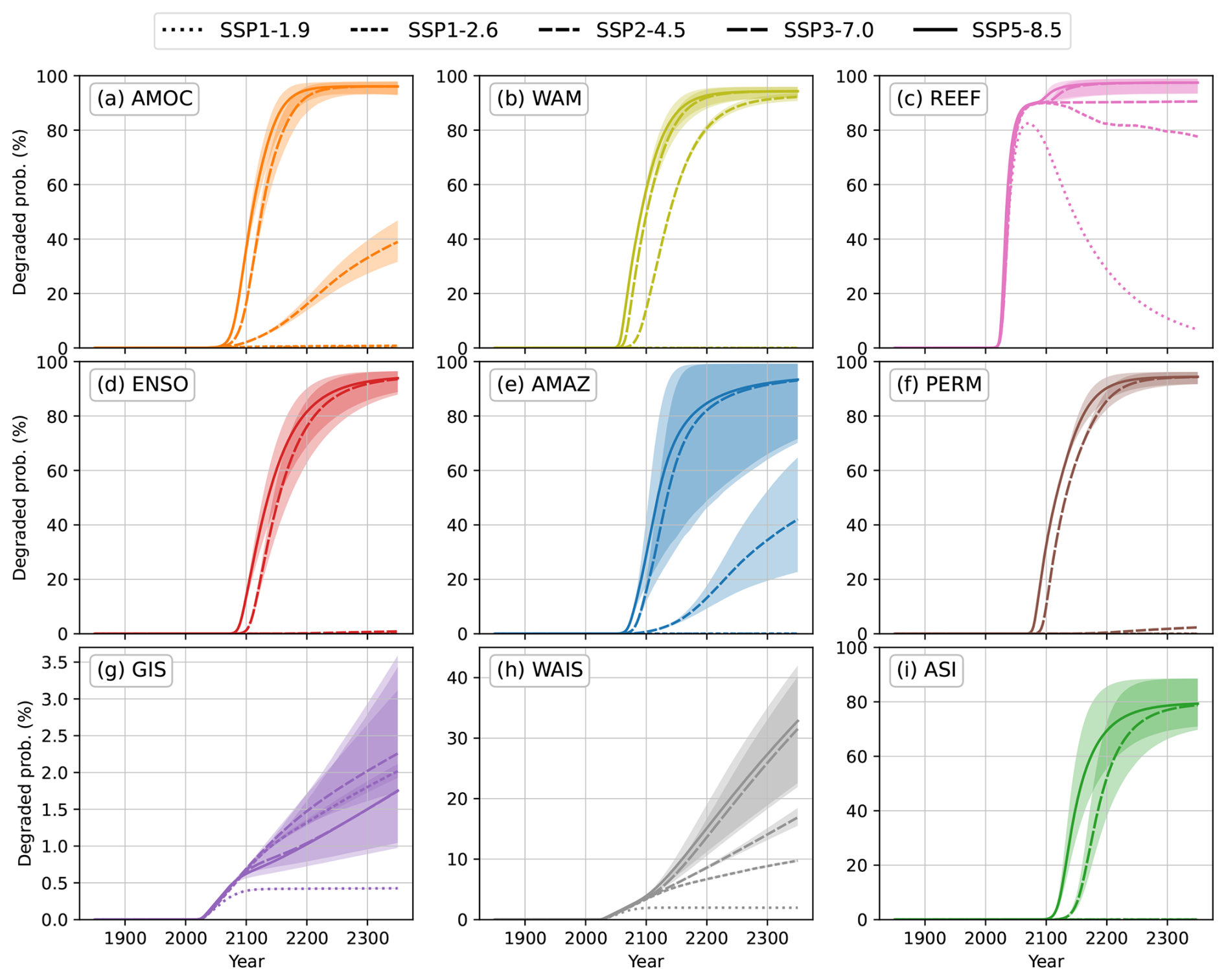
Figure 4 Ensemble mean of degraded probability of interacting tipping elements and ENSO over time under different global warming scenarios, relative to 1850–1900 (Morice et al., 2021; Lee et al., 2021). In particular, for the years 1850–2014 historical warming is used while from 2015–2350 the projected global warming trajectories are used. Note the y axis scales are different for the two ice sheets in panels (g) and (h) than the other 7 panels. For graphical clarity, only the 5- to 95-percentile uncertainty range of the ensemble are included, moreover comparisons to the interaction-free case has been left to Fig. 6.

3.3 Short term risks under the extended shared-socioeconomic pathways

While the stable stationary distribution highlights the long term risks for each tipping element, given that global warming level is fixed in time, the short term evolution (up to multi-centennial times) is of most importance to policy and human life. For instance, it took the Earth less than a century to reach an annual GMST of +1.6 °C in 2024 (Copernicus Climate Change Service, 2025) from around +0.25 °C in 1950 (Lee et al., 2021). In this section, therefore, using both historical levels of global warming (1850–2014) and future projections (2015–2350) under the five extended shared-socioeconomic pathways (SSPs) outlined in the IPCC's Sixth Assessment Report (Lee et al., 2021), we look at how the risk of each tipping element evolves over the course of 500 years (from 1850 to 2350). As different SSPs represent different policy and commitment scenarios for the 21st century onwards, we can see in Fig. 4, in particular, how different tipping elements respond, in essence, to human activity.

As the dynamics are dominated by the faster timescales of GMST evolution rather than the slower timescales of an individual element's recovery or collapse, which SSP scenario the tipping elements are subjected to has a huge impact on the risk of being Degraded certainly by 2350 and even in 2100 for some. For instance, under the fossil-fuelled scenario of SSP5-8.5, in which exploitation of global resources are intensified and lifestyles become increasingly energy-intensive, the Sahel and West African monsoon (WAM) has a 58 % likelihood on average to be Degraded in 2100 and is very likely (94 %) to be so in 2350. On the other hand, under the sustainable and “green” development pathway of SSP1-1.9, where ecologies are preserved, planetary boundaries respected and income inequality being actively reduced, on average WAM is exceptionally unlikely (< 0.003 %) to be degraded. Suffice to say, in all cases, following such a green and sustainable scenario minimises the risk of degrading tipping elements, as compared to other scenarios.

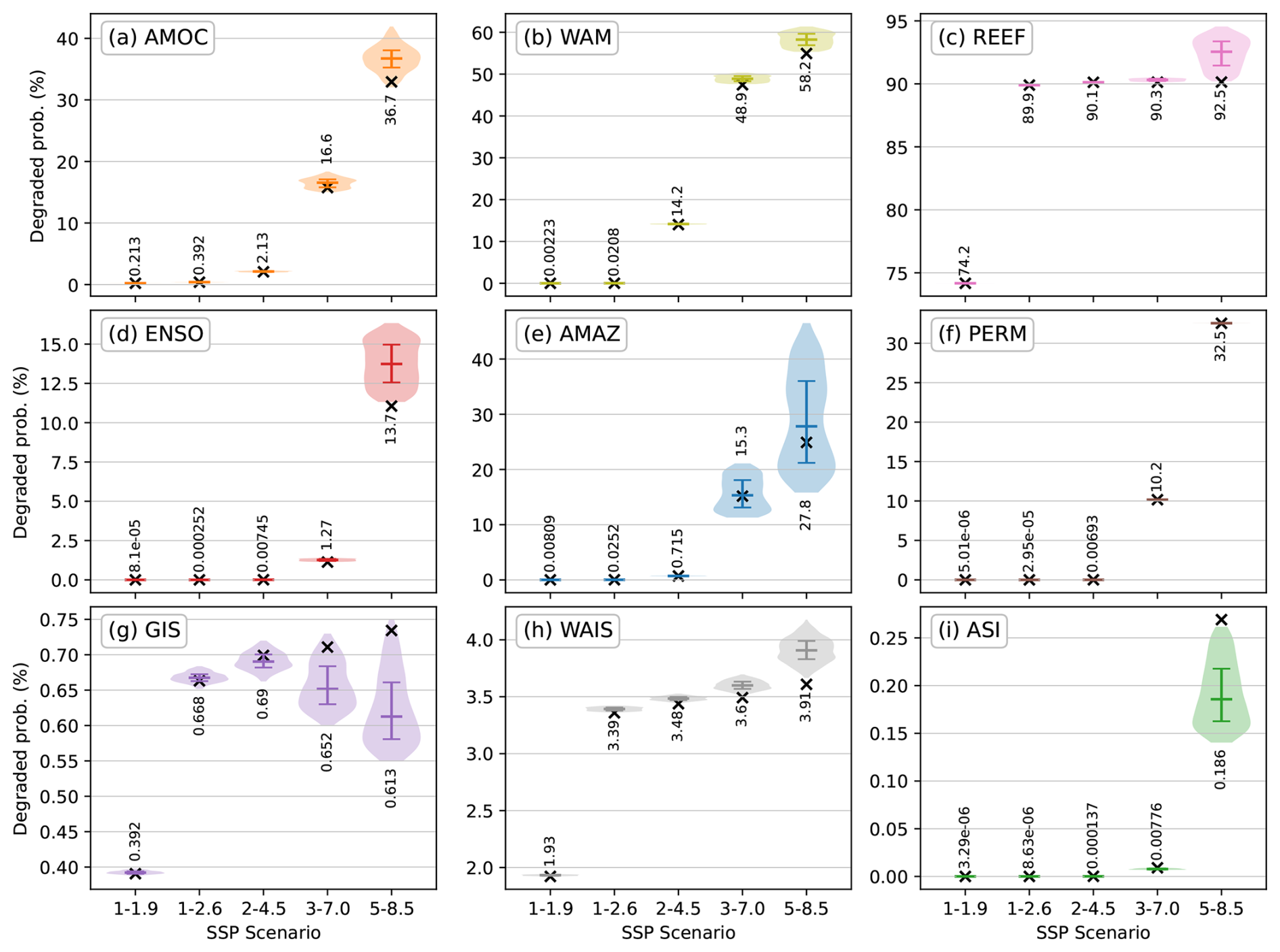
Figure 5 Distribution of Degraded risks of interacting tipping elements under different global warming scenarios by the year 2100. In particular, in each panel, each violin plot shows the distribution over the ensemble of plausible interaction matrices, with bars indicating the interquartile range and median, whose value is further indicated. Black crosses meanwhile indicate the interaction-free degraded risks, also evaluated at 2100.

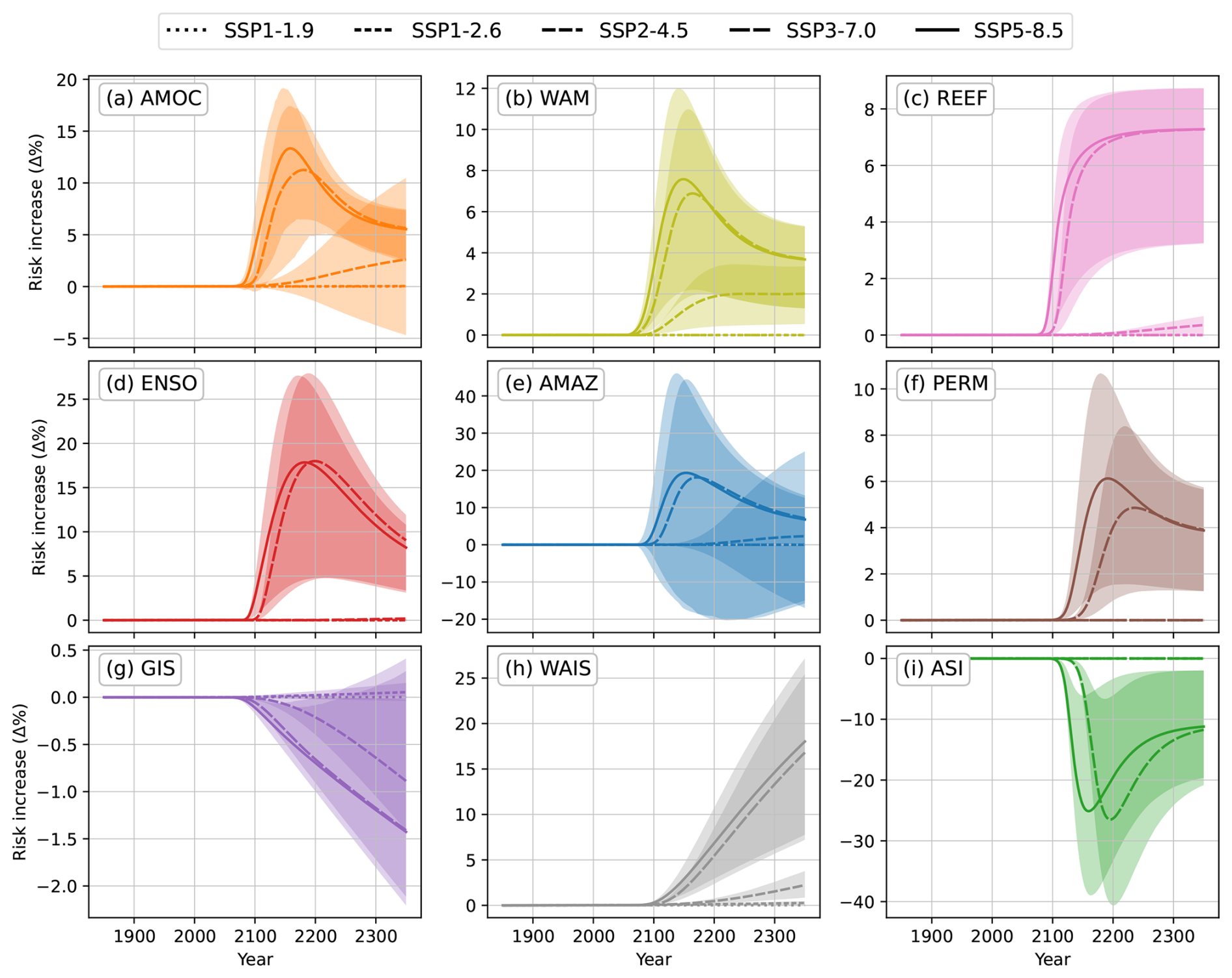
Figure 6 Increase in the probabilities of the tipping elements and ENSO being degraded, due to their interactions, relative to the interaction-free case, over time under different global warming scenarios. In particular, the bold line represents the historical scenario in the years 1950–2014 while from 2015–2350 the different styles of line represent different extended shared-socioeconomic pathways (SSPs). For graphical clarity, only the 5- to 95-percentile uncertainty range of the ensemble are included.

That being said, under the most optimistic scenario SSP1-1.9, the coral reefs are at least likely to be degraded (> 74 %) in 2100 (see Fig. 5 due to the initial overshoot in temperature and their decadal collapse times. Fortunately, as the overshoot is temporary, the coral reefs are able to recover sufficiently quickly that by 2350 (see Fig. S2 in the Supplement) they are very unlikely (< 10 %) to remain degraded. Under the middle-of-the-road scenario, SSP2-4.5, its risk does begin to fall in 2100–2150 but remains likely to be degraded by 2350, unlike AMOC and the Amazon whose risks increase an intermediate amount under the same scenario from 2100 onwards. Although the reefs' singular interaction from ENSO does destabilise it over time, the increase from the interaction-free case is less than 1 % for the first three scenarios and almost 7 % for SSP3-7.0 and SSP5-8.5 (see Fig. 6); the vast majority of its risk is due to its fast timescales (a few decades) and to its low tipping threshold (+1.5 °C). On the other hand for very slow tipping elements their dynamics are dominated instead by the evolution of SSP warming and their faster neighbours. For instance, GIS, which evolves over millennia, is stabilised quickly enough by AMOC, which evolves over decades to centuries, such that its 2100 risk is actually reduced by around 1 % for the hotter scenarios. Intriguingly, under both SSP1 scenarios, the ensemble mean risk is instead slightly increased, though by a very small amount, although some interaction matrices still result in a reduction.

We find that, on the one hand, AMOC is at worst about as likely as not (40 %) to be degraded by 2100 under SSP5-8.5, despite the inclusion of other, mostly destabilising, interactions – depending on the SSP scenario this risk may be even less than 5 %. On the other hand, by 2350, we can see how dependent the risk of tipping is on the specific SSP scenario, with the two hottest scenarios (SSP3-7.0 and SSP5-8.5) leading to AMOC being very likely to tip, while under both SSP1 scenarios the risk is negligible. We find that interactions on the whole play a destabilising role in AMOC though these effects are most prominent only after 2100, increasing the risk by 10 %–15 % on average and by up to 18 % (see Fig. 6). Although, under the other 3 scenarios, some interaction matrices can reduce the tipping risk by up to 5 % in 2350 – and thus somewhat stabilise AMOC as for instance Sinet et al. (2025) claimed – we find that the destabilising interactions not considered by Sinet et al. (2023, 2024) dominate the stabilising effects of WAIS producing a net increase in risk by 2350 across all scenarios.

Although this subsystem cannot sufficiently stabilise itself nor the entire network (see Fig. S4 in the Supplement), individual tipping elements are less at risk, in large part due to the stabilising effects from AMOC. For instance, for equilibrium temperatures hotter than 2 °C, GIS is on average less likely to tip than without interactions. The effect can be as large as a reduction of 10 %–20 % in absolute value at equilibrium (see Fig. S1). In the short term too, especially after 2100, interactions lower the risk by up to 2 %, depending on the scenario (see Fig. 6). Moreover due to its millennial timescales and despite its lower threshold of 1.5 °C, GIS is very unlikely to tip (< 3.5 %) across all scenarios by 2350, thus allowing for some safe overshoots in temperature as has been previously found (Ritchie et al., 2021; Wunderling et al., 2023). Similarly, the Arctic sea ice too is stabilised greatly by the AMOC, both at equilibrium (by up to 20 %) and in the short term (for the SSPs 3-7.0 and 5-8.5 the reduction is most prominent in the period 2150–2200 at around 20 %–30 %).

In fact for all elements barring the coral reefs and polar ice sheets, we see that the effects of interactions under SSP3-7.0 and SSP5-8.5 are most strongly felt between 2150–2200 in Fig. 6 and gradually weaken past 2200. Meanwhile, the effects of interactions plateau for the coral reefs, since they are already maximally at risk under SSP3-7.0 and SSP5-8.5. Given their millennial timescales, the strength of the effects of interactions increase slowly over time across all SSPs for both polar ice sheets. In general, interactions play a much smaller role for all climate subsystems under SSP1-1.9, SSP1-2.6 and even the middle of the road scenario of SSP2-4.5 for most, since temperatures are, first, too low to impact the important nodes in the network (i.e. to begin network-wide cascades). Second, the tipping points that are crossed under these 3 scenarios are either sink nodes in the network (the coral reefs) so does not impact others, or are too slow to respond to begin a cascade.

4 Conclusions

4.1 Core findings

In this work, we have presented our novel risk assessment framework, modelling 8 interacting tipping elements and ENSO under various global warming scenarios and at equilibrium. In summary, we find that interactions, on the whole, increase the risk of individual climate subsystems being degraded, similarly to Wunderling et al. (2021a, 2023). Moreover, we quantify the effects of interactions by comparing against an interaction-free baseline, unlike Wunderling et al. (2023), finding that, at the level of total risk, the net effect due to interactions is actually somewhat weak, for example as seen in Fig. 2. Despite the fact that the majority of pairwise interactions are destabilising (Wunderling et al., 2024), we find that the few strongly stabilising interactions (namely those due to the collapse of AMOC) offset much of this total risk, but not entirely. For the Greenland ice sheet and the Arctic sea ice the decrease in their respective risks can be as much 30 % at equilibrium (Fig. S1) while in the short term the latter can feel up to a 40 % decrease in risk under SSP3-7.0 and SSP5-8.5.

With respect to AMOC, conceptual models (Sinet et al., 2023, 2024) and Earth System models (Sinet et al., 2025), linking the polar ice sheets to the AMOC via meltwater flux, have found that AMOC can effectively be stabilised depending on the collapse rates of and time delay between tipping of the two polar ice sheets, even without the cooling effects a weakening AMOC has on the Greenland ice sheet (Jackson et al., 2015). However, at the inclusion of more interactions and other tipping elements, we find, in contrast, that AMOC is on the whole destabilised by its overall interactions, especially after the year 2100 in the short term (Fig. 6) and above 1.5 °C of global warming at equilibrium (Fig. S1).

Considering a robust representation of interactions, global warming temperature is still a critical factor in the risk of tipping element degradation. We find that keeping long term temperatures below 1.5 °C – less than the lower limits of the Paris Agreement – risks fewer than 3 degraded tipping elements (the coral reefs and both polar ice sheets), while in the short term “taking the green road” (Riahi et al., 2017) in global development and economic paradigms can completely avoid any tipping risks. In particular, as exemplified by the SSP1-1.9 scenario (Lee et al., 2021) – one of the most optimistic overshoot scenarios – temporary overshoots in temperature mean that the coral reefs will be very likely (94 %) to be in their prosperous state by 2350, despite being, first, likely (74 %) to be degraded in 2100.

Although large tipping risks can be avoided by limiting the convergence temperature – for long-term GMST under 1 °C, we find that all climate subsystems considered are very unlikely to be degraded, similarly to Wunderling et al. (2023) – we are still well above such temperatures, having reached 1.6 °C in 2024 (Copernicus Climate Change Service, 2025) and likely entering a 20 year period with an average of at least 1.5 °C (Bevacqua et al., 2025). Our stylised model study suggests that we are already close to having up to 3 tipped elements – the coral reefs (> 90 %), the Sahel and West African monsoon (> 48 %) and the AMOC (up to 36.7 %) – by 2100. By 2350 under the SSP3-7.0 and SSP5-8.5 scenarios, this total risk drastically increases to an equivalent of almost 7 tipped elements (all except the Greenland ice sheet and perhaps the West Antarctic ice sheet). Moreover, we find that even if global warming temperatures are permanently maintained within the Paris Agreement limits of 1.5–2 °C, on average 3 elements (the coral reefs and the polar ice sheets) will still be degraded at equilibrium, suggesting that such limits be treated only as short-term overshoot limits which cannot be sustained in the long term.

4.2 Limitations

Our framework differs from other stylised models on interacting tipping elements (Gaucherel and Moron, 2017; Sinet et al., 2023, 2024; Wunderling et al., 2021a, 2023) as we model the interactions more coherently to the limited data, originally quantified from expert elicitation (Kriegler et al., 2009) as probability factors, while greatly expanding the set of elements to those found by Wunderling et al. (2024). In following this conceptual logic, the probability to collapse is inversely-proportional to (and therefore non-linear in) stabilising interactions while remaining a linear polynomial in the destabilising interactions. However, since state variables of the dynamical systems models and the degraded state in our model are not necessarily linear, then linear interactions in probability space may not correspond to linear interactions in state variable space. Moreover, compared to the simple Boolean model of Gaucherel and Moron (2017), a big advancement of our approach is an explicit inclusion of timescales and temperature-dependence in the tipping process. Stylised models, including ours, are useful to complement physics-based models while physically based ESMs should, reciprocally, be used to complement and inform conceptual models.

We acknowledge that the models of Wunderling et al. (2021a, 2023) are more suitable to explain other phenomena such as critical slowing down, while explicitly including bifurcations. However, these models conceptualise interactions deterministically as opposed to the explicitly probabilistic interactions discussed in Kriegler et al. (2009). Furthermore, they are more computationally demanding. We use a 2-state Markov chain as a higher level abstraction of the double-fold bifurcations to gain a more computationally efficient and ultimately more interpretable model fit for a risk assessment framework. The outcomes of our model qualitatively reflect their results while being computationally cheaper and remaining coherent to the original expert elicitation. For our ensemble of 500 interaction matrices, numerically solving for the long-term risk of all tipping elements simultaneously across 10⁴ values of temperature took 15 min on a personal computer. For the short-term risk over all SSP scenarios all simulations took less than 5 s to compute.

Although we have an explicit temperature dependence for collapse, we do not do so for recovery, due to the deep uncertainty within the literature. In some climate subsystems, such as the polar ice sheets (Armstrong McKay et al., 2022), strong hysteresis lead to threshold effects for recovery that may not occur at the same temperature value as the corresponding collapse threshold. In others, even the question of reversibility is still under debate, let alone having a fully quantified temperature dependence. For example, while Lenton et al. (2025) note a growing amount of evidence to suggest Arctic sea ice loss is irreversible, they find it is not yet sufficient to assess it as such. Therefore, we try to remain as agnostic as possible with respect to the temperature dependence of recovery, minimising the amount of additional assumptions, by assuming temperature independence, in this paper. We suspect in the short-term (multi-centennial scales) that temperature-dependent recovery will not change our results greatly, given the extra order of magnitude in the recovery timescales, however the effects in the long term and at equilibrium may be large – dominating any effects due to interactions – and warrants further detailed investigation.

Another major limitation was the (lack of) data regarding interactions themselves, in particular in their quantification. Although Wunderling et al. (2024) is a substantial review, the strength of each interaction is qualitatively assessed. While some of these interaction strengths were quantified in the earlier expert elicitation of Kriegler et al. (2009), others were reassessed or were entirely new in the 2024 review, and thus lacked any quantification. In order to synthetically fill the data gap, we had converted qualitative strengths into numerical values (see Appendix A2), potentially introducing additional errors and uncertainty.

More fundamentally, interactions between tipping elements simply have received little attention in the broader literature. As seen in Fig. 3, some interactions can affect a subsystem's risk to be degraded by 10 % (ENSO's effects on the coral reefs) and even by up to 30 % (AMOC's effects on the Greenland ice sheet). To that extent, a missing interaction could change the results, particularly for individual subsystems, by a large amount. Expert elicitations can help to coalesce large scant parts of the literature over multiple models and might even provide insights into events not captured well by Earth system models (Lam and Majszak, 2022), however the lack of explicit inclusion of general climate model results and/or historical observations speak to their limited reliability more generally.

4.3 Future research direction

Fortunately, more research is being devoted to tipping points in the Earth system, of which our work is one. One major set of works are the Global Tipping Points (GTP) Reports (Lenton et al., 2023, 2025) that extensively focus on all aspects and variety of tipping points. The set of interactions evaluated in the latest 2025 report is bigger than Wunderling et al. (2024) (as they include interactions with the North Atlantic subpolar gyre and the Southern Ocean), however there was no longer any mention of the strength of the interactions, let alone a qualitative evaluation, again highlighting the need for more research regarding inter climate subsystem interactions.

Another international collaboration is the the Tipping Points Modelling Intercomparison Project (TIPMIP) (Winkelmann et al., 2025) which seeks to systematically asses tipping risks using state-of-the-art coupled Earth system models, following the success of the Coupled Model Intercomparison Projects (CMIPs) used for climate projections. As these large projects continue to output detailed and complex models and simulations – some of the preliminary Tier 1 results and experimental protocols of TIPMIP are being released – it will be important to compare the outputs of those models to our simplified framework, given the significant difference in computational and time costs. At the conceptual and mathematical level, it will also be important to draw a more rigorous equivalence between the stylised bifurcation-driven models for individual/interacting elements (e.g. the Stommel, 1961, model) and our probabilistic approach, in order to derive more realistic and process-based transition rates. Moreover, given the importance of long transients, for example as can be found in AMOC (Mehling et al., 2024), more research is needed to quantify the timescales associated with transitions to and from intermediate states in order to, say, model each climate subsystem as some N-state Markov chain with more complex transitions and for N>2.

While the coral reefs are at most risk both at equilibrium and in the short term, they form a sink node in the interaction network, with only incident edges, that affects no other nodes in the network, and thus any intervention or policy directed at them would be limited in effect only to the reefs. A long-term and sustainable policy must instead take into account and consider the entire network. For example, we find that AMOC has the highest betweenness centrality (Freeman, 1977), regardless of the network instantiation, further supporting the findings of Wunderling et al. (2021a) and Lenton et al. (2025) that AMOC is a dominant mediator of tipping cascades. Given limited resources, AMOC might therefore be an effective node to intervene on first, in our stylised network model. On the other hand, we stress, once again, the critical importance of limiting global warming and global emissions of CO₂ and other short-lived climate pollutants. Future work is needed, therefore, to rigorously test how interventions on single nodes affect the short- and long-term dynamics of the entire Earth system network.

Finally, in this work, we have used the SSP warming scenarios as proxies for the potential effects of humans on the environment and ecology. However, given how complex social-environmental relationships are, it is necessary to integrate agency more directly. To conclude, we note that eco-evolutionary games (Tilman et al., 2020), multi-agent reinforcement learning dynamics in stochastic games (Barfuss et al., 2019, 2020, 2025), and networked and spatial games (Bara et al., 2024) are promising frameworks to do so. Our networked model lays the groundwork for future works that consider the social dilemma of interacting Earth tipping elements and climate subsystems.

Appendix A: Data methods

A1 Parameter inference from threshold and timescale estimates

Our individual tipping element data is based on the work of Armstrong McKay et al. (2022), who had reviewed 33 tipping elements. However in our work, due to the limited amount of TE interaction data available (Wunderling et al., 2024), we consider only nine of the 33 tipping elements – 6 global core tipping elements, 2 regional elements (low-lattitude coral reefs and the Sahel and West African monsoon) and El Niño-Southern Oscillation (ENSO) whose status as a tipping element has been disputed (Collins et al., 2019; Lee et al., 2021).

Lenton et al. (2023)

Table A1 (Ir)reversibility of individual tipping elements as reproduced from the Global Tipping Points Report 2023 (Lenton et al., 2023).

In some cases model parameters can be directly taken from the original dataset; the collapse timescale τ_c,i is precisely the “Timescale (y) – Est.” while the midpoint of the logistic response function T_lim,i is given by the “Threshold (°C) – Est.”. In the event there is no estimate, for either parameter, then the average of the upper and lower bounds can be used instead – for example although there is no threshold estimate for ENSO, it has a minimum temperature of 3.0 and 6.0 °C, hence we estimate T_lim,i = 4.5 °C.

Given climate model limitations and the historical rarity of a tipping point collapsing into a degraded state – let alone recovering from one back into the prosperous state – very little data, almost none, exists regarding the recovery timescales. Instead of numerical values for specific recovery timescales, the Global Tipping Points Report 2023 (Lenton et al., 2023) instead considered whether a tipping element was “irreversible”, at least over decadal or centennial times. For instance the polar ice sheets (with high confidence) and the Amazon rainforest (with medium confidence) are considered “irreversible”, while the coral reefs are thought to only be irreversible (with medium confidence) over decadal timescales. On the other hand the Arctic winter sea ice is considered reversible (with medium confidence) even at these shorter timescales. In this work, therefore, we assume an order of magnitude difference between the collapse timescales and the recovery timescales which are sufficient to meet the (ir)reversibility conditions summarised in the Global Tipping Points Report (see Table A1).

Finally for the logistic growth rate parameters β_i of each tipping element we utilise the literature derived bounds for the threshold temperature. For all considered tipping elements, lower bounds for the threshold estimate exist, and as such we we fix β_i such that the collapse response function is 0.001 at the lower bound and 0.5 at the threshold estimate. Mathematically this reduces to, for $\mathit{\sigma }(T_{\text{min},i};{\mathit{\beta }}_i)={\mathit{\sigma }}_{\text{min}}$, such that we can solve for ${\mathit{\beta }}_i=\log ({\mathit{\sigma }}_{\text{min}}^{-\mathrm{1}}-\mathrm{1})/(T_{\text{lim},i}-T_{\text{min},i})=\log \left(\mathrm{999}\right)/(T_{\text{lim},i}-T_{\text{min},i})$.

A2 Probability factors between tipping elements

While the individual data of tipping elements are largely quantitive the extended data set for TE-TE interactions of Wunderling et al. (2024) are qualitative. In particular for each pairwise TE-TE interaction (i.e. edge), Wunderling et al. (2024) had summarised their extensive literature review into four qualitative variables (for details see their Table 1 and Fig. 3): Response (Destabilising, Stabilising or Unclear); Response strength (Strong, Moderate, Weak or Unclear); Agreement within literature (High, Medium or Low); Evidence (Robust, Medium, Limited or Very Limited).

Much of their interactions, however, are based on the original, quantitative expert elicitations (Kriegler et al., 2009), from which, in an earlier work, Wunderling et al. (2021a) had converted into edge weights for their dynamical systems model (for details see their Table 2). Comparing these values to the qualitative interactions of the later work (Wunderling et al., 2024) allows us to reverse engineer a mapping from the qualitative interactions into probability factors, thus effectively extending the set of probability factors from Kriegler et al. (2009). Roughly speaking, the response type determines the sign of the edge, i.e. whether the edge would contribute to either the numerator or denominator in Eq. (5), while the response strength affected the maximum possible weight of the edge. We clean the dataset slightly by discarding edges whose type and strength are both unclear, thus removing the (ENSO, AMOC) and (AMOC, Indian summer monsoon) edges, as there was no unambiguous way to coherently include them. In so doing this also entirely disconnects the Indian summer monsoon from the rest of interaction network, as it has no other edges and will therefore neither be affected by or affect the other tipping elements, at least according to the review (Wunderling et al., 2024).

For some qualitative strengths there is a clear, consistent correspondence between the probability factor value and qualitative strength, while others have been revised. Take the GIS-AMOC interaction as an example: Kriegler et al. (2009) found it had a maximum probability factor of 10, meaning the probability to collapse of AMOC increases by a factor of 10 if GIS collapses, while Wunderling et al. (2024) evaluated the interaction as strong and destabilising. On the other hand, the GIS-WAIS interaction which Kriegler et al. (2009), and therefore Wunderling et al. (2021a), was considered strong with a maximum probability factor of 10, was revised in the later work of Wunderling et al. (2024) to only being of moderate, though still destabilising, effect.

Kriegler et al. (2009)Wunderling et al. (2021a)Wunderling et al. (2024)

Table A2 Table of interactions including the minimum and maximum possible values for their edge weights. In our work, each interaction has weight w_ij which is uniformly distributed from a minimum weight m_ij to a maximum weight M_ij, in other words $w_{ij}\sim U(m_{ij},M_{ij})$. The sign of the weight corresponds to the sign of the corresponding signed edge ($a_{ij}^{\pm }$) while the magnitude of the weight is the value of the signed edge, in other words $a_{ij}^{\text{sgn}\left(w_{ij}\right)}=\left|w_{ij}\right|$. For reference and comparison, we also tabulate the response type and/or strength discussed in three previous references, namely: the probability factors (PF) from Kriegler et al. (2009); the maximum link strengths that Wunderling et al. (2021a) had inferred from the probability factors; and the updated literature-based assessment from Wunderling et al. (2024) in terms of response type and strength.

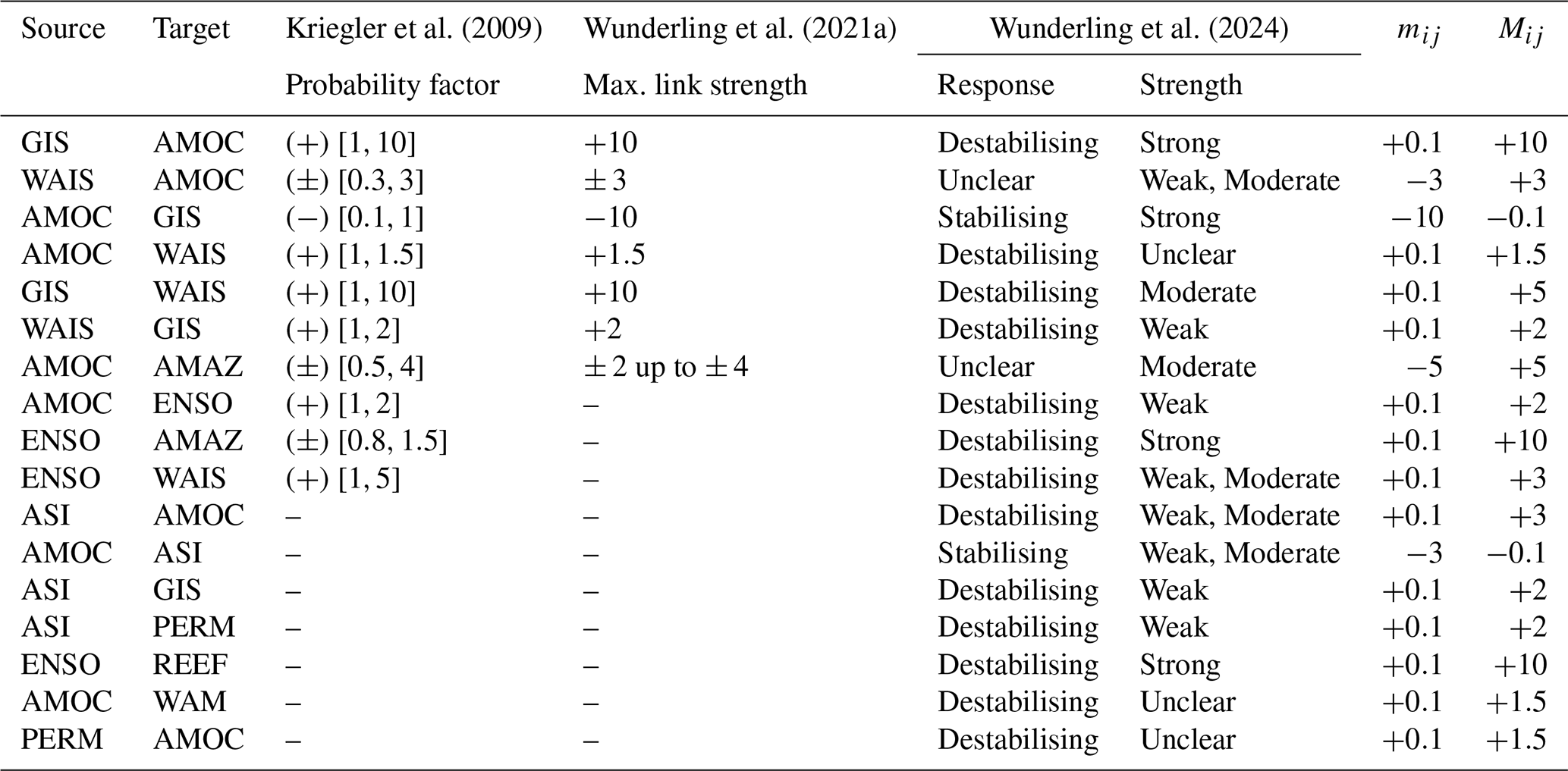
To this end, we use the few interactions which are consistent throughout all three references, to make an equivalence between the qualitative strength to edge weight in our model. For example, AMOC-GIS corresponded to a PF of 0.1, in other words the probability to collapse of GIS is reduced by a factor of 10 given that AMOC has tipped. Wunderling et al. (2024) also evaluated this as strong and stabilising. Therefore we make the equivalence that a “strong” interaction would have have a maximum absolute edge weight of 10. In doing so, we have tried to limit adding our own subjective belief of individual interaction strengths, by utilising this more systematic method.

For each TE-TE interaction we randomly sample a weight $w_{ij}\sim U(m_{ij},M_{ij})$ whose distribution is parametrised by a minimum m_ij and maximum M_ij; the maximum absolute value is given by the response strength – “Strong” = 1; “Moderate” = 0.5; “Weak, Moderate” = 0.3; “Weak” = 0.2; “Unclear” = 0.15 – while the sign of the weight is given by the response type – “Destabilising” is positive, “Stabilising” is negative, “Unclear” can be either. Similarly edges with a clear type will have a minimum absolute value of with sign given by the edge type; unclear edges have a minimum absolute value equal to the negative of the maximum absolute value. Table A2 summarises the distributions of w_ij using the data from Table 1 and Fig. 3 of Wunderling et al. (2024). Finally, with respect to our signed networks, edge (i,j) is destabilising (stabilising) if w_ij>0 (w_ij<0), with edge weight $\left|w_{ij}\right|$. In this way TE-TE interactions with unclear responses can either have stabilising or destabilising edges, depending on the sampling.

A3 Warming under Shared Socioeconomic Pathways

The Shared Socioeconomic Pathways (SSPs) are a variety of potential scenarios for climate change under different global socioeconomic changes. In particular the five used in this work were produced in the IPCC Sixth Assessment Report (AR6) (Lee et al., 2021; Fyfe et al., 2021; Intergovernmental Panel on Climate Change (IPCC), 2023) and represent different large-scale narratives in terms of sustained global efforts to counter climate change. In particular, similarly to Armstrong McKay et al. (2022), we use the mean global surface temperature anomaly, relative to 1850–1900, though we use the extended scenarios, with historical data (1950–2014) and the projections (2015–2350) under 5 different SSPs. For the sake of clarity, we have displayed only simulation results that evolve under the mean global surface air temperature (GSAT) under the SSPs.

Appendix B: Computational methods

B1 Interaction matrices

Given the uncertainty regarding the 17 different TE-TE interactions, we utilise a 17-dimensional Latin hypercube sample (McKay et al., 1979) in order to give a better coverage of the 17-dimensional parameter space, using the LatinHypercube class of the SciPy Python package (Virtanen et al., 2020). In particular we take 500 samples using this method, each one representing a different instance of a 9 × 9 interaction adjacency matrix. For consistency and comparison we use the exact same ensemble in both the short-term and long-term risk analysis. Any ensemble statistic – e.g. mean, quantiles, etc. – are based on these 500 interaction matrices. In contrast, the interaction-free treatment needed no ensemble as, in effect, the adjacency matrix of independently evolving tipping elements is the zero matrix 0.

B2 Long- and short-term risk simulations

For the nine climate subsystems we consider, Eq. (10) gives 9 simultaneous equations that we solve numerically using the fsolve function of NumPy Python package to derive the joint stationary distributions (i.e. the long term risk) for a range of global warming temperatures in [0,10] °C with incremental steps of 0.001 °C, for each of the 500 interaction matrices of the ensemble, as well as for the interaction-free case.

In the short-term case, we simulate using the update equation in Eq. (6), the evolution of each tipping element annually given each of the 500 interaction matrices and the 5 extended SSPs. For the years 1850–2014 (inclusive) the historical levels of global warming were used, while all tipping element risks were initialised to $D_i\left(\mathrm{1850}\right)=\mathrm{0},\forall i$. For the years 2015–2250 (inclusive), the 5 SSP scenarios continue from the historical scenario both in temperature and the individual risk of each element.

Since degraded-risks are bounded ($D\in [\mathrm{0},\mathrm{100}]$ %), the underlying distribution of such risks cannot be Normal- nor t-distributed. As such we do not report confidence intervals per se – that is the interval above and below the ensemble (sample) mean in which 90 % of the time the true population mean would be captured, assuming the samples are Normal- or t-distributed – since these may produce intervals which are not strictly within the bounds. Instead we report ranges within certain percentiles of the ensemble, such that the 5- to 95-percentile range, for example, covers the middle 90 % of ensemble simulations.

Appendix C: Mathematical Derivations

C1 Convergence times Eq. (12)

Consider a 2-state Markov chain with probability to collapse p and probability to recover is q. Its probability to be degraded D(t) evolves via Eq. (3) and has equilibrium solution D_∗ given by Eq. (4). Let t_ϵ be the convergence time to the equilibrium solution, in other words the first time step at which $t_{\mathit{ϵ}}=min\mathit{\{}t:|D\left(t\right)-D_{\ast }|<\mathit{ϵ}\mathit{\}}$. Assuming $p+q<\mathrm{1}$, D(t) monotonically increases with time t towards D_∗ so that we can approximate t_ϵ as occurring once $\left|D\right(t)-D_{\ast }|=\mathit{ϵ}$. Given our parametrisation assumptions from the real data (that the recovery time is ten times the collapse time) we can simplify $p=\mathrm{1}/(\mathit{\tau }+\mathrm{1})$ and $q=\mathrm{1}/(\mathrm{10}\mathit{\tau }+\mathrm{1})$.

$$\begin{array}{ll}{\displaystyle }\left|D\right(t_{\mathit{ϵ}})-D_{\ast }|& {\displaystyle }={\left(\mathrm{1}-{\displaystyle \frac{\mathrm{1}}{\mathit{\tau }+\mathrm{1}}}-{\displaystyle \frac{\mathrm{1}}{\mathrm{10}\mathit{\tau }+\mathrm{1}}}\right)}^{t_{\mathit{ϵ}}-\mathrm{1}}=\mathit{ϵ}\\ {\displaystyle }\ln \mathit{ϵ}& {\displaystyle }=(t_{\mathit{ϵ}}-\mathrm{1})\ln \left(\mathrm{1}-{\displaystyle \frac{\mathrm{1}}{\mathit{\tau }+\mathrm{1}}}-{\displaystyle \frac{\mathrm{1}}{\mathrm{10}\mathit{\tau }+\mathrm{1}}}\right)\\ {\displaystyle }\ln \mathit{ϵ}& {\displaystyle }=(t_{\mathit{ϵ}}-\mathrm{1})\ln \left(\mathrm{1}-{\displaystyle \frac{\mathrm{11}\mathit{\tau }+\mathrm{2}}{(\mathrm{10}\mathit{\tau }+\mathrm{1})(\mathit{\tau }+\mathrm{1})}}\right)\\ {\displaystyle }{t}_{\mathit{ϵ}}-\mathrm{1}& {\displaystyle }={\displaystyle \frac{\ln \mathit{ϵ}}{\ln (\mathrm{1}-x)}}\end{array}$$

where $x=(\mathrm{11}\mathit{\tau }+\mathrm{2})/\left(\right(\mathrm{10}\mathit{\tau }+\mathrm{1}\left)\right(\mathit{\tau }+\mathrm{1}\left)\right)<\mathrm{1}$ for τ>1. Since x<1 we can use the following series expansion for $\mathrm{1}/\ln (\mathrm{1}-x)$,

$$\begin{array}{ll}{\displaystyle \frac{\mathrm{1}}{\ln (\mathrm{1}-x)}}\approx & {\displaystyle }-{\displaystyle \frac{\mathrm{1}}{x}}+{\displaystyle \frac{\mathrm{1}}{\mathrm{2}}}+{\displaystyle \frac{x}{\mathrm{12}}}+O\left(x^{\mathrm{2}}\right)\\ {\displaystyle }=& {\displaystyle }-{\displaystyle \frac{\mathrm{10}{\mathit{\tau }}^{\mathrm{2}}+\mathrm{11}\mathit{\tau }+\mathrm{1}}{\mathrm{11}\mathit{\tau }+\mathrm{2}}}+{\displaystyle \frac{\mathrm{1}}{\mathrm{2}}}\\ {\displaystyle }& {\displaystyle }+{\displaystyle \frac{\mathrm{1}}{\mathrm{12}}}\left({\displaystyle \frac{\mathrm{1}}{\mathrm{10}\mathit{\tau }+\mathrm{1}}}+{\displaystyle \frac{\mathrm{1}}{\mathit{\tau }+\mathrm{1}}}\right)+O\left({\displaystyle \frac{\mathrm{1}}{{\mathit{\tau }}^{\mathrm{2}}}}\right)\\ {\displaystyle }\approx & {\displaystyle }-\left({\displaystyle \frac{\mathrm{10}\mathit{\tau }}{\mathrm{11}}}+{\displaystyle \frac{\mathrm{101}}{\mathrm{121}}}-{\displaystyle \frac{\mathrm{1}}{\mathrm{11}\mathit{\tau }}}\right)+{\displaystyle \frac{\mathrm{1}}{\mathrm{2}}}+{\displaystyle \frac{\mathrm{1}}{\mathrm{12}}}{\displaystyle \frac{\mathrm{11}}{\mathrm{10}\mathit{\tau }}}\\ {\displaystyle }& {\displaystyle }+O\left({\displaystyle \frac{\mathrm{1}}{{\mathit{\tau }}^{\mathrm{2}}}}\right)\\ {\displaystyle }=& {\displaystyle }-{\displaystyle \frac{\mathrm{10}\mathit{\tau }}{\mathrm{11}}}-{\displaystyle \frac{\mathrm{81}}{\mathrm{242}}}+{\displaystyle \frac{\mathrm{241}}{\mathrm{1320}\mathit{\tau }}}+O\left({\displaystyle \frac{\mathrm{1}}{{\mathit{\tau }}^{\mathrm{2}}}}\right)\end{array}$$

where the first line can be derived either through a Laurent expansion or through a Taylor expansion first of $\ln (\mathrm{1}-x)=-{\sum }_{n=\mathrm{1}}^{\mathrm{\infty }}(x^n/n)$ followed by a Binomial expansion. This lets us approximate t_ϵ in terms of the collapse time τ.

$$t_{\mathit{ϵ}}\approx \mathrm{1}+\left({\displaystyle \frac{\mathrm{10}}{\mathrm{11}}}\mathit{\tau }+{\displaystyle \frac{\mathrm{81}}{\mathrm{242}}}-{\displaystyle \frac{\mathrm{241}}{\mathrm{1320}\mathit{\tau }}}\right)\ln \left({\displaystyle \frac{\mathrm{1}}{\mathit{ϵ}}}\right)$$