An EOF-Based Emulator of Means and Covariances of Monthly Climate Fields

Fast emulators of comprehensive climate models are often used to explore the impact of anthropogenic emissions on future climate. A new approach to emulators is introduced that generates means and covariances of monthly averaged climate variables as a function of global mean surface temperature. The emulator is trained with output from a state-of-the-art climate model and serves as a good first-order representation for the evolution of spatially resolved climate variables and their variability. To train the emulator, data is first projected into a reduced-dimensional space; the emulator then learns the dependence of climate variables on global mean surface temperature in the projected space. To recover climate variables in physical space, an inverse transformation is applied. The resulting emulator can cheaply generate means and variances of climate fields averaged over arbitrarily defined regions and in previously unseen warming scenarios. For illustrative purposes, the emulator is applied to predict changes in the mean and variability of monthly values of both surface temperature and relative humidity as a function of global mean surface temperature changes. However, the approach can be applied to any other variable of interest on yearly, monthly or daily timescales.

1 Introduction

In the study of climate change, it is crucial to explore the response of the Earth system to a variety of possible future greenhouse gas emission scenarios and quantify the uncertainties associated with future projections. Despite their limitations, state-of-the-art Earth System Models (ESMs), such as those participating in the Climate Model Intercomparison Project (CMIP,  Eyring et al., 2016), remain our most reliable tools for estimating the Earth system response to increased greenhouse gas concentrations. These large-scale models aim to represent as many aspects of the climate system as faithfully as possible. However, because of the high computational and material costs of running ESMs, these models can only simulate the Earth system response to a few potential future scenarios (Tebaldi et al., 2021a). On the other hand, studies of climate mitigation and adaptation strategies often seek to explore a wide range of possible solutions, creating a need for methods to compare localized impacts across a wide range of emissions scenarios (O'Neill et al., 2016b; Waidelich et al., 2024). Our work provides a framework for extending projections of future climate scenarios beyond those simulated with ESMs. The method captures spatially coherent changes at any scale in both the mean and variance of climate variables in response to user-defined warming scenarios.

Emulators of ESMs have been gaining popularity as a way to facilitate access to climate projections. Here, we consider the class of emulators trained on the output of ESMs to cheaply and quickly predict the climate response to arbitrary climate change scenarios. We will not consider other types of emulators that are being actively pursued for other applications, including climate model downscaling, parametrization of subgrid-scale processes, and model parameter calibration (e.g, Doury et al., 2023; Li et al., 2019; Lai et al., 2025; Peatier et al., 2022; Tebaldi et al., 2025). From here on, the term emulator will refer exclusively to the class of emulators trained to extend ESMs to arbitrary future scenarios. The importance of these emulators is likely to rise due to the increasing computational demands of ESMs: their ever refining spatial resolution, their growing complexity (as embodied by the number of model components and their sophistication), the use of more accurate numerical methods (Griffies et al., 2020; Souza et al., 2023; Taylor et al., 2023; Silvestri et al., 2024), and the push to run larger ensembles of simulations differing in initial conditions (Schneider et al., 2024, 2023). Emulators are necessary to both compress existing information into a more manageable form as well as to bridge the gap between the computational demand of running a full ESM and the computational hardware available to everyday consumers of climate information. This need is best illustrated by the evidence that projections of future emissions are updated every year, while a new deck of ESM simulations by CMIP takes close to a decade to generate and organize for community sharing.

The simplest and most common emulation technique is pattern scaling (Santer and Wigley, 1990; Huntingford and Cox, 2000; Mitchell, 2003). Pattern scaling estimates spatially resolved changes in climate variables by linearly regressing local variables on global mean surface temperature or cumulative emissions. While pattern scaling has been shown to have remarkable skill in emulating projected changes in local mean temperatures (Santer et al., 1990; Lütjens et al., 2025), it has no inherent probabilistic component and is less accurate for other climate variables (Tebaldi and Arblaster, 2014; Tebaldi and Knutti, 2018; Kravitz and Snyder, 2023). Recent work has been dedicated to constructing machine learning-based climate emulators (e.g. Watson-Parris et al., 2022; Kitsios et al., 2023; Yu et al., 2024; Christensen et al., 2024) to move beyond the linear assumption inherent in pattern scaling. However, questions remain about their overall skill compared to linear pattern scaling (Lütjens et al., 2025). Additionally, their lack of interpretability and the computational cost of model training may limit their applications. The emulator discussed in this work is rooted in the paradigm of statistical emulation as a function of globally averaged surface temperature (e.g., pattern scaling) rather than in the alternative paradigm of autoregressive emulation that predicts the evolution of climate variables or of their statistics as a function of initial conditions (e.g., autoregressive machine learning models). In particular, we aim to emulate spatially averaged second-order statistics of variables of interest given a specified future value of globally averaged surface temperature.

Our focus on emulating variability stems from the recognition that a shift in a climate variable is significant only if it lies outside the bounds of the internal variability inherent in the system. Internal variability has been shown to dominate uncertainty in climate projections over a decade for regional temperature and over much longer periods for other variables, like regional precipitation (Hawkins and Sutton, 2009, 2011). The concept of time of emergence (ToE) is used to quantify when a climate signal becomes statistically distinguishable from internal variability (Hawkins and Sutton, 2012; Tebaldi and Friedlingstein, 2013). In its simplest form, ToE is defined as the first time a climate variable (e.g., ensemble mean temperature globally or at a point) exceeds a threshold derived from internal variability (often the ensemble variance), which may itself evolve under climate change. The interest in ToE and related questions (such as climate attribution and projection uncertainty) underpins the need for emulators to capture both mean trends and internal variability.

Significant work has been dedicated to the extension of linear pattern scaling to account for both internal variability in the climate system and structural uncertainty in ESMs. A common approach is to take a large ensemble of climate simulations, either from a single model or from a multi-model set, and apply pattern scaling separately to each simulation, deriving a measure of uncertainty from the resulting ensemble spread (Tebaldi and Knutti, 2018; Zelazowski et al., 2018; Gao et al., 2023; Kravitz and Snyder, 2023). Generally, examining ensemble spread within a single model is among the most reliable ways of quantifying the internal variability of the climate system, while inter-model spread includes structural uncertainty (Collins and Allen, 2002; Tebaldi and Knutti, 2007; McKinnon and Deser, 2018; Tebaldi et al., 2021b; Lehner et al., 2020). Other statistical emulators have gone beyond pattern scaling to explicitly include stochastic components to mimic the climate system's inherent variability (Alexeeff et al., 2018; Beusch et al., 2020; Link et al., 2019; Nath et al., 2022). For example, researchers have augmented pattern-scaling frameworks with residual resampling or autoregressive processes, ensuring that emulator outputs exhibit the same spatio-temporal covariance structure and ensemble spread as the original ESM runs (Link et al., 2019; Nath et al., 2022; Tebaldi et al., 2022). The MESMER emulators (Beusch et al., 2020; Nath et al., 2022) have applied approximate methods (Gaussian copulas) to compute the covariances among different climate variables and locations.

Our emulator design for averaged climate fields marries the pattern scaling approach with a statistical model of internal variability that can account for spatial and cross-variable correlations. This is achieved with a generative data-driven emulation method for spatially resolved climate fields, applied in this work to monthly temperature and relative humidity. As a first step, the ESM training data is projected into a reduced-dimensional space using empirical orthogonal function (EOF) decomposition (Hannachi et al., 2007). We then model the evolution of the means and covariances of the data in this reduced-order space as a function of global mean surface temperature. To recover projected statistics, a reverse transformation is applied that maps the means and covariances of EOF amplitudes into the means and variances of climate variables in physical space. In designing our emulation approach, we prioritized computational efficiency in order to improve the accessibility of the emulator for users and applications without access to significant computational resources.

The main innovation of our method is the balance of simplicity alongside robustness in modeling the lower-order statistics of the system. This includes modeling the full EOF covariance matrices, which are necessary to compute changes in variance and correlations of climate variables over arbitrary geographical regions. Covariances between locations are required to estimate variability on a region beyond the size of an original model grid cell (e.g., the variability over Sub-Saharan Africa is much larger if all regions experience the same temperature fluctuations than if they are all independent). Additionally, covariances between different variables are essential for quantifying the impact of internal variability on climate projections and to assess compound risks (e.g., high temperature and relative humidity are more problematic than high temperature and low relative humidity).

The climate emulator literature includes models on many timescales, ranging from yearly to monthly to daily. The temporal resolution required depends on the specific application of the emulator. In this work, we use monthly data for illustrative purposes; our approach to emulation could be applied to other temporal resolutions as well, as in Wang et al. (2025). Projections of monthly climate statistics are important for understanding a number of impacts of climate change, such as changes in the seasonal cycle, water management, and other phenomena of agricultural relevance (Guo et al., 2002; Odjugo, 2010; Schlenker and Roberts, 2009; Mishra and Singh, 2010; Stéfanon et al., 2012). Furthermore, some emulators with finer temporal resolution, such as the one in Bassetti et al. (2024), require monthly projections as input; our emulator could thus be used as pre-conditioning information. Importantly, by emulating statistics beyond the mean, our emulator provides additional information that may be used to condition downstream models or aid in decision-making (e.g., via uncertainty quantification through emulated ensemble spread). Such a modular emulation pipeline is common, as illustrated by the MESMER family of emulators (Beusch et al., 2020; Nath et al., 2022; Quilcaille et al., 2022, 2023).

We condition our emulator on the global, ensemble, and yearly mean surface temperature, which we refer to as “global mean temperature” for short. This procedure is common among other emulators of spatially-resolved climate variables (e.g., Osborn et al., 2016; Alexeeff et al., 2018; Goodwin et al., 2020). Global mean temperature has been found to scale approximately linearly with cumulative emissions (Matthews et al., 2009; Masson-Delmotte et al., 2021), at least for smoothly-growing emissions (Giani et al., 2025) and ignoring, e.g., the time-lagged response to radiative forcing, or the impact of short-lived aerosols and nonlinear feedbacks like those from melting ice. This simple relationship underpins the utility of a global mean temperature-based emulator. However, one could easily go further by relying on Simple Climate Models (e.g. Meinshausen et al., 2011; Lembo et al., 2020; Leach et al., 2021; Bouabid et al., 2024; Dorheim et al., 2024) to translate arbitrary emission pathways into novel trajectories of global mean temperature. Our emulator would then use these trajectories to generate realizations of spatially resolved monthly variables under those emission scenarios, continuing in line with the modular emulation framework. We comment that often the global mean temperature anomaly from a preindustrial period is used rather than the actual global mean temperature, but here we will use the absolute global mean temperature.

A sufficiently large ensemble of initial conditions is necessary to infer non-stationary statistical information. For this reason, we choose to emulate the evolution of climate variables generated by a CMIP-class model, specifically MPI-ESM1.2 LR (v1.2.01p7) (Mauritsen et al., 2019; Olonscheck et al., 2023), that ran a large ensemble (50 members) of simulations for a number of emissions scenarios (see Sect. 2 for details). We emphasize that throughout this work, when referring to an ensemble or ensemble mean, we are considering only a single-model ensemble (e.g., an initial-condition ensemble). We do not intend for these methods to be applied to multi-model ensembles. We illustrate our approach for two variables: surface temperature and surface relative humidity. Still, the approach is agnostic to the variables being emulated. It can easily be applied to any variables from a single ESM ensemble, so long as their EOF amplitude statistics are mostly described by their means and covariances. While in this work we emulate each of the two variables separately, our approach is also applicable to the joint emulation of several variables with minimal modification, which we discuss in Sect. 3.

Our paper is organized as follows: in Sect. 2, we introduce the dataset used in this work. Sect. 3 discusses the EOF-based coarse-graining procedure applied to the data. In Sect. 4, we discuss the details of the emulator design and the regression problem. In Sect. 5, we show the emulator's ability to replicate the data's statistics under climate change. In Sect. 6, we illustrate one possible application of the emulator using a case study. Finally, in Sect. 7, we discuss the broader implications of this work and propose future directions for constructing complementary emulator models.

2 Data

To train our emulator, we use the output from the MPI-ESM1.2-LR (v1.2.01p7) ESM model (Mauritsen et al., 2019; Olonscheck et al., 2023), which contributed to CMIP6. We chose this model because of the large number of simulations (ensemble members) it ran for each emission scenario: 50 simulations are run for each scenario, differing only in their initial conditions. A large ensemble is necessary to separate a model's internal variability from the anthropogenic signal (Collins and Allen, 2002; Tebaldi et al., 2021b; Lütjens et al., 2025). In the CMIP6 model set, only three ESMs submitted ensembles of 30 or more members: MPI-ESM1.2-LR, EC-Earth3, and CanESM5. Among these, the MPI model is the only one with an equilibrium climate sensitivity to greenhouse gas emissions within the “likely” range determined by multiple lines of evidence (Hausfather et al., 2022) and with the entire ensemble available for open download.

Analysis performed in Lütjens et al. (2025) on the same MPI dataset suggests that an emulation method that uses polynomial fitting for projecting changes in climate variables as a function of space, such as ours, captures the evolution of the ensemble mean variables even if trained on a few ensemble members (in terms of emulation error). However, an ESM with many ensemble members is necessary to train the emulation of internal variability (Tebaldi et al., 2021b). How many members constitute a “large enough” ensemble will depend on the particular variable(s) being targeted and the application being considered. For present purposes, the ESM training data must contain sufficient ensemble members to accurately represent the climate internal variability, i.e., the variance and cross-correlation of the climate variables of interest. Lütjens et al. (2025) finds that an ensemble size of at least 10 members is necessary to capture the internal variability of temperature and precipitation. This is consistent with our finding that 30 ensemble members are sufficient for the training of our emulator.

Each MPI-ESM1.2-LR ensemble member is run for the historical period, spanning 165 years between 1850–2014, and for various future warming scenarios spanning the 86 year future period 2015–2100. We consider output from simulations of three future scenarios from the ScenarioMIP experiments: SSP5-8.5, SSP2-4.5, and SSP1-1.9. The ScenarioMIP experiments are plausible futures corresponding to different climate mitigation and cooperation narratives (O'Neill et al., 2016a; Tebaldi et al., 2021a). Figure 1 reports the global mean temperature profiles of the historical period and the three future scenarios considered in this work for each of the 50 MPI-ESM1.2-LR ensemble members.

Figure 1 Yearly global mean temperature in the MPI-ESM1.2-LR model ensemble. Each dashed line represents one of 50 initial-condition ensemble members, and the solid line shows the ensemble mean. Different colors correspond to the historical 1850–2014 period and the three future scenarios considered in this study: SSP5-8.5, SSP2-4.5, and SSP1-1.9. The future period spans 2015–2100. The historical period lasts 165 years, and the future period – 86 years.

Our goal is to develop an emulator that predicts changes in the mean and covariance of climate fields as a function of emissions. The first step in the process is to represent the statistics as a function of (or, more appropriately, conditioned on) global, ensemble, and yearly mean temperature and hence cumulative emissions (see Masson-Delmotte et al., 2021). As mentioned above, the ensemble mean is calculated over a single model with multiple realizations. Following standard practice, we will refer to the global, ensemble, and yearly mean surface temperature as “global mean temperature” throughout the text, denoted ${\stackrel{\mathrm{‾}}{T}}_{\mathrm{g}}$.

We select the historical experiment and the SSP5-8.5 high-warming scenario for training the emulator because together they span the widest range of global mean temperatures. This leaves SSP2-4.5 and SSP1-1.9 as the validation sets for regression, see Sect. 5. SSP2-4.5 features milder monotonic warming that levels off at the end of the century (through the elimination of emissions), while SSP1-1.9 features a peak in global mean temperature around mid-century followed by a decrease to end-of-historical-period temperatures by 2100 (as a consequence of negative emissions), see Fig. 1. Because we are developing an emulator conditioned only on global mean temperature from a scenario with monotonically increasing emissions (without accounting for emissions history or other memory effects), it is important to test its performance in scenarios with non-monotonic emissions. Such scenarios are of ever-increasing interest to mitigation and adaptation studies and policy. We emphasize that our approach is purely data-driven and should not be used to extrapolate statistics in climates outside of its global mean temperature training range.

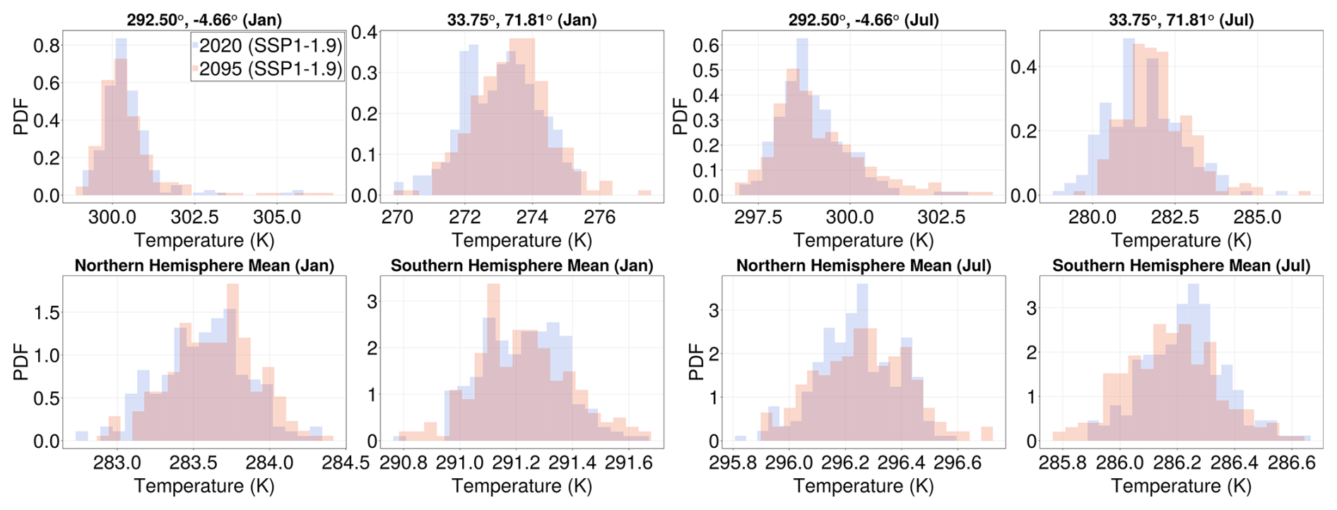
Figure 2 Surface temperature histograms of the non-monotonic SSP1-1.9 scenario corresponding to similar global mean temperatures (${\stackrel{\mathrm{‾}}{T}}_{\mathrm{g}}$ = 289.3 K) but for two different time intervals: 2018–2022 (blue bars) and 2093–2097 (red bars). Histograms are constructed for selected locations (top row) and hemisphere averages (bottom row) and for January (left) and July (right). The histograms mostly overlap, lending support to the choice of parameterizing the distributional change (and hence lower-order statistical changes) for a fixed month with only ${\stackrel{\mathrm{‾}}{T}}_{\mathrm{g}}$.

To presume that time-dependent climate statistics for different emissions scenarios can be parameterized by a state-dependent (i.e., time-independent or history-independent) scalar quantity is a strong assumption but one that is justified a posteriori for the cases considered in this work, see Fig. 2 and, later on, Figs. 7 and 8. Figure 2 shows histograms of surface temperature data in the MPI model for selected locations (top row) and hemisphere averages (bottom row) in January (left) and July (right). Two 5 year windows in the SSP1-1.9 future scenario are compared: 2018–2022 (in blue) and 2093–2097 (in red). The SSP-1.1.9 scenario is non-monotonic, and these two periods correspond to similar global mean temperatures of around ${\stackrel{\mathrm{‾}}{T}}_{\mathrm{g}}$ = 289.3 K, separated by an intermediate 70 year period of higher temperatures. We observe that, for the most part, the histograms for the two periods overlap. We thus conclude that a state-dependent parametrization of climate statistics is not unreasonable for our purposes.

Before delving into the specific details of the emulator formulation, it is crucial to first understand the underlying rationale guiding our approach. Our key assumption is that the statistics of climate system fields, in our case the EOF modal amplitudes a (see Sect. 3), can be represented by a probability density for every possible state, with time and emissions history replaced by the global mean temperature ${\stackrel{\mathrm{‾}}{T}}_{\mathrm{g}}$ and seasonal information such as the month m:

$$\begin{array}{}\text{(1)}& \mathit{\rho }(\mathit{a},t|\text{ emissions})\to \mathit{\rho }\left(\mathit{a}|{\stackrel{\mathrm{‾}}{T}}_{\mathrm{g}},m\right).\end{array}$$

This assumes that conditioning on global mean temperature serves as an informative parametric form to characterize the changing distribution of the climate-relevant quantities. In the application described in the following sections, we do not consider the full probability distribution and instead assume that only the first two moments – means and covariances – can be represented as functions of global mean temperature.

We illustrate our approach for monthly mean surface (2 m) temperature and monthly mean surface (2 m) relative humidity. These are the “tas” and “hurs” variables, respectively, in the CMIP6 nomenclature. The MPI-ESM1.2-LR model has a horizontal resolution in the atmosphere of 1.8°. We use the model output on its original 192 × 96 lat-lon grid. We calculate the global mean temperature (used to condition the emulator) by globally averaging the 2 m temperature variable.

3 Coarse-Graining

We coarse-grain the representation of the temperature and relative humidity fields, using Empirical Orthogonal Functions (EOFs) as a dimensionality reduction technique (Lorenz, 1956; Kutzbach, 1967; Barnston and Livezey, 1987a); see Hannachi et al. (2007) for a comprehensive review of the technique's history. EOF modes have been shown to effectively capture the dominant patterns of variability of the Earth system (Barnston and Livezey, 1987b; Hannachi et al., 2007). EOF decomposition has been used in previous emulator work for both dimensionality reduction (Holden and Edwards, 2010; Holden et al., 2015; Yuan et al., 2021) and more generally as a method of generating an uncorrelated projection basis (Link et al., 2019). More recently, Falasca et al. (2025) and Falasca et al. (2024) have demonstrated how modal amplitudes of large-scale patterns (under the additional assumption that they can be approximated as multivariate Gaussian distributions) can be used to interpret patterns of variability and teleconnections through data-driven approaches.

The EOF modes are ranked according to the fraction of overall variability they capture. The leading EOF modes represent patterns that span large geographical regions. While EOF modes can, with some limitations (Monahan et al., 2009), be interpreted physically, here they are only used as a dimensionality reduction technique. Using a subset of leading EOF modes as a fixed-in-time orthogonal basis for the projection of ESM data, we shall model the statistics (means and variances) of EOF amplitude coefficients as a function of global mean temperature.

We compute the EOF basis ϕ through a singular value decomposition of our data in the historical period of one of the ensemble members. The resulting basis constitutes 165 × 12 = 1980 EOFs ordered by the magnitude of the singular values. We discard the last 980 basis functions, leading to a total of 1000 basis functions ${\mathit{\varphi }}_i\left(\mathit{x}\right),i\in [\mathrm{1},\mathrm{1000}]$. The notation (x), which we use throughout this work, indicates that EOF basis functions are spatially resolved, i.e., functions of the location x. We use the same basis set for all months and compute EOFs separately for each variable of interest. We project data from every scenario and every ensemble member onto our constant basis. Because we are using the EOF modes as a basis for dimensionality reduction, the choice of using only one ensemble member to generate the basis and keeping the basis fixed throughout the emulation process significantly reduces the computational cost of the emulator. The specific ensemble member used was found to not impact the performance of the resulting emulator. We further emphasize that because the EOFs are used as basis onto which data are projected, we do not require any assumptions about the structure of the EOFs or their stationarity over time. Indeed, the method described in the following section is agnostic to the specific choice of dimensionality reduction technique.

Although in this work we emulate each variable separately, our method may also be used to emulate the joint evolution of two or more climate variables. To do so, one would only need to concatenate the multiple variables into one super-variable (after, perhaps, properly normalizing them) before proceeding with the emulation technique as described for a single variable, now on the super-variable. The only difference between the single- and multiple-variable cases is the need for extra care in constructing the EOF basis. When performing a singular value decomposition, the resulting modes are ranked in order of decreasing percent of variance captured. For a single variable, the leading EOFs are thus easily interpretable as a sort of set of dominant modes. In contrast, in the multiple-variable case, the modes will capture the dominant modes of joint-variable variability, but not necessarily those of the individual variables. Depending on the particular set of variables and intended applications, one must assess whether the resulting EOF basis is capturing the desired variability and how many leading modes one should accordingly retain. We emphasize, however, that the purpose of the EOF decomposition is dimensionality reduction, and any set of basis functions is suitable for the purpose of emulation, but a poor choice of EOFs may result in a useless, albeit accurate, emulator.

The choice to work with the leading EOFs is not only one of convenience to reduce the data size. It is also motivated by evidence that the projections of climate models are more reliable at larger scales (Gleckler et al., 2008). Finer-scale details captured by high-order EOFs–such as full temperature distributions at a point–are better modeled using different approaches, such as downscaling from coarse-grained information. In probabilistic jargon, we divide the set of modal amplitudes a into modes corresponding to large-scale coarse structures a_C and “fine-scale modes” a_F. The probability distribution for climate variables (for a fixed global mean temperature ${\stackrel{\mathrm{‾}}{T}}_{\mathrm{g}}$ and month m) can then be decomposed as the product of two conditional distributions:

$$\begin{array}{}\text{(2)}& \mathit{\rho }\left({\mathit{a}}_{\mathrm{C}},{\mathit{a}}_{\mathrm{F}}|{\stackrel{\mathrm{‾}}{T}}_{\mathrm{g}},m\right)=\mathit{\rho }\left({\mathit{a}}_{\mathrm{F}}|{\mathit{a}}_{\mathrm{C}},{\stackrel{\mathrm{‾}}{T}}_{\mathrm{g}},m\right)\mathit{\rho }\left({\mathit{a}}_{\mathrm{C}}|{\stackrel{\mathrm{‾}}{T}}_{\mathrm{g}},m\right).\end{array}$$

Our work focuses on approximating the means μ and covariances 𝓒 of $\mathit{\rho }\left({\mathit{a}}_{\mathrm{C}}\right|{\stackrel{\mathrm{‾}}{T}}_{\mathrm{g}},m)$, the distribution of a_C as a function of the global mean temperature ${\stackrel{\mathrm{‾}}{T}}_{\mathrm{g}}$ and month m. Armed with the means and covariances of the modes a_C, one can then reconstruct means and variances of the original fields both locally or averaged over some area, as we will see in Sect. 4.2. In addition, if the statistics of the variables of interest are Gaussian, means and covariances are sufficient to reconstruct the whole probability density functions (see Appendix A).

Approximating fine-scale structures conditioned on coarse-grained variables, i.e., approximating $\mathit{\rho }\left({\mathit{a}}_{\mathrm{F}}\right|{\mathit{a}}_{\mathrm{C}},{\stackrel{\mathrm{‾}}{T}}_{\mathrm{g}},m)$, is left to future work. In downscaling exercises, it is typically assumed that

$$\begin{array}{}\text{(3)}& \mathit{\rho }\left({\mathit{a}}_{\mathrm{F}}|{\mathit{a}}_{\mathrm{C}},{\stackrel{\mathrm{‾}}{T}}_{\mathrm{g}},m\right)\approx \mathit{\rho }\left({\mathit{a}}_{\mathrm{F}}\right|{\mathit{a}}_{\mathrm{C}}),\end{array}$$

i.e., information about the coarse scales may be sufficiently informative to parameterize the distribution of the fine scales.

4 Regression

After projecting the ESM data into the EOF space, we model the EOF coefficients as a function of global mean temperature (see also Holden and Edwards, 2010; Bruckner et al., 2003) and proceed to emulate their means and covariances. The method can be applied to any variables regardless of their distributions insofar as one is only interested in the means and covariances of any linear functional of the variable field, see Sect. 4.2. Despite not requiring a Gaussian approximation, we will often overlay histograms of variables from the MPI model with Gaussian distributions with the means and covariances generated by our emulator. This is an arbitrary, yet somewhat constrained choice because a Gaussian distribution is among the most natural ways to visualize a distribution parameterized solely by its mean and variance. It so happens, however, that the EOF amplitudes of monthly average temperature and relative humidity have approximately Gaussian distributions. This is to be expected from the multivariate version of the central limit theorem, which states that any variable that is the average of many independent realizations of the same process has a Gaussian distribution. In our case, we average in time, over a month, and in space by the coarse-graining implied by the EOF decomposition. See Appendix A for further discussion.

We are now ready to describe our emulation approach in detail. Section 4.1 describes the procedure for fitting to data, and Sect. 4.2 describes how to utilize the emulator and its relation to pattern scaling.

4.1 Emulator Details

Following the EOF-based dimensionality reduction of the ESM training data, we develop and train a stochastic emulator of spatially resolved monthly temperature and relative humidity fields. As stated previously, obtaining the set of estimated EOF coefficients $\widehat{\mathit{a}}$ requires estimating a mean $\widehat{\mathit{\mu }}$ and covariance $\widehat{\mathcal{C}}$ as a function of global mean temperature ${\stackrel{\mathrm{‾}}{T}}_{\mathrm{g}}$ and month index m, i.e.,

$$\begin{array}{}\text{(4)}& \widehat{\mathit{\mu }}\left({\stackrel{\mathrm{‾}}{T}}_{\mathrm{g}},m\right)\text{ and }\widehat{\mathcal{C}}\left({\stackrel{\mathrm{‾}}{T}}_{\mathrm{g}},m\right).\end{array}$$

Since each month is modeled separately, we will drop the notation m with the implicit understanding that any regression is for a fixed month. Throughout this work, we use the notation $\widehat{\cdot }$ to denote an emulator-derived estimate of a quantity, in contrast to the ESM-derived “ground truth”. The large ensemble of MPI model simulations offers a robust way to estimate the means and covariances since we view, for a fixed month and year, every individual ensemble member as a realization of a high-dimensional distribution parameterized solely by the month and global mean temperature.

The dependence of the means $\widehat{\mathit{\mu }}$ on ${\stackrel{\mathrm{‾}}{T}}_{\mathrm{g}}$ is modeled as a quadratic function

$$\begin{array}{}\text{(5)}& \widehat{\mathit{\mu }}={\widehat{\mathit{\mu }}}_{\mathrm{0}}+{\widehat{\mathit{\mu }}}_{\mathrm{1}}{\stackrel{\mathrm{‾}}{T}}_{\mathrm{g}}+{\widehat{\mathit{\mu }}}_{\mathrm{2}}{\stackrel{\mathrm{‾}}{T}}_{\mathrm{g}}^{\mathrm{2}}.\end{array}$$

Figure 3 Regression of mean (top row) and covariance (bottom row) of the surface temperature EOF amplitudes as a function of global, ensemble, and yearly mean temperature in January. Estimates from the MPI model ensemble simulations are shown as purple points, while the blue lines are the emulator fits. The quadratic fits capture both the linear trends and the slight curvature.

This approximation yields a better overall fit than a linear function, see Fig. 3 and Appendix B. Higher-order polynomial fits could be used to improve on the results presented here but may also overfit the data.

Modeling the covariance of the EOF coefficients as a function of global mean temperature requires more care. When fitting the mean of each EOF mode, one can use standard methods for curve fitting, such as least squares. Parameterizing a covariance matrix as a function of global mean temperature is more subtle since all the matrix entries must conspire together to yield a symmetric positive definite matrix. We thus choose to represent the dependence of the covariance matrices $\widehat{\mathcal{C}}$ on ${\stackrel{\mathrm{‾}}{T}}_{\mathrm{g}}$ as

$$\begin{array}{}\text{(6)}& \widehat{\mathcal{C}}=\widehat{\mathit{L}}{\widehat{\mathit{L}}}^T\text{ and }\widehat{\mathit{L}}={\widehat{\mathit{L}}}_{\mathrm{0}}+{\widehat{\mathit{L}}}_{\mathrm{1}}{\stackrel{\mathrm{‾}}{T}}_{\mathrm{g}}.\end{array}$$

This functional form guarantees that $\widehat{\mathcal{C}}$ is symmetric positive definite because it is the product of a matrix $\widehat{\mathit{L}}$ and its transpose. In Eq. (6) each entry of $\widehat{\mathit{L}}$ is modeled as a linear function of ${\stackrel{\mathrm{‾}}{T}}_{\mathrm{g}}$, leading to a quadratic model for the covariance:

$$\begin{array}{}\text{(7)}& \widehat{\mathcal{C}}\left({\stackrel{\mathrm{‾}}{T}}_{\mathrm{g}}\right)={\widehat{\mathit{L}}}_{\mathrm{0}}{\widehat{\mathit{L}}}_{\mathrm{0}}^T+\left({\widehat{\mathit{L}}}_{\mathrm{0}}{\widehat{\mathit{L}}}_{\mathrm{1}}^T+{\widehat{\mathit{L}}}_{\mathrm{1}}{\widehat{\mathit{L}}}_{\mathrm{0}}^T\right){\stackrel{\mathrm{‾}}{T}}_{\mathrm{g}}+{\widehat{\mathit{L}}}_{\mathrm{1}}{\widehat{\mathit{L}}}_{\mathrm{1}}^T{\left({\stackrel{\mathrm{‾}}{T}}_{\mathrm{g}}\right)}^{\mathrm{2}}.\end{array}$$

As with the means, it is possible to go beyond a linear representation for $\widehat{\mathit{L}}$, though one would run the risk of overfitting. We experimented with a variety of possible models to emulate the covariance structure and found that this model allows for maximal flexibility with minimal required assumptions. This parametric form yields a representation of how the internal variability changes as a function of global mean temperature, and hence time and emissions scenario (under appropriate assumptions).

To find ${\widehat{\mathit{L}}}_{\mathrm{0}}$ and ${\widehat{\mathit{L}}}_{\mathrm{1}}$ we minimize the loss function

$$\begin{array}{}\text{(8)}& \text{Loss}\left({\widehat{\mathit{L}}}_{\mathrm{0}},{\widehat{\mathit{L}}}_{\mathrm{1}}\right)=\sum _{{\stackrel{\mathrm{‾}}{T}}_{\mathrm{g}}}{∥\widehat{\mathcal{C}}\left({\stackrel{\mathrm{‾}}{T}}_{\mathrm{g}}\right)-\mathcal{C}\left({\stackrel{\mathrm{‾}}{T}}_{\mathrm{g}}\right)∥}^{\mathrm{2}},\end{array}$$

where $\widehat{\mathcal{C}}$ is given by Eq. (7) and $\Vert \cdot \Vert$ is an appropriately chosen norm. In our case, we used a Frobenius norm (minimizing the square distance between each matrix entry), but other choices would likely yield good answers as well. This minimization was performed in JAX (Bradbury et al., 2018), on an H100 NVIDIA GPU using automatic differentiation and Kingma and Ba (2014)'s “ADAM” for optimization. The minimization was initialized with a constant covariance matrix, i.e., $\stackrel{\mathrm{‾}}{\mathcal{C}}=\frac{\mathrm{1}}{\mathrm{251}}{\sum }_{\text{year }=\mathrm{1850}}^{\mathrm{2100}}\mathcal{C}\left(\text{year}\right)$. This choice was implemented by taking ${\widehat{\mathit{L}}}_{\mathrm{1}}=\mathrm{0}$ and obtaining ${\widehat{\mathit{L}}}_{\mathrm{0}}$ from the Cholesky factorization of $\stackrel{\mathrm{‾}}{\mathcal{C}}$. To perform the regression for the covariance matrix, we used the fact that the covariance can be computed separately for each year (over the set of all ensemble realizations) and each year has an associated global mean temperature.

We illustrate the result of the regression procedure for surface temperature in Fig. 3. The top row represents the regression for the ensemble mean EOF coefficients, and the bottom row shows the regression problem for the covariance matrix between EOF modes, both for January. We first describe the top row. The purple dots are the projected modal amplitudes for a few sample EOFs plotted at each year for all ensemble members of the MPI data for the historical and SSP5-8.5 scenario. The bottom row is obtained by calculating the covariance between sample modal amplitudes for each year separately using all ensemble members. These data are then regressed against each year's global, ensemble, and temporal mean of surface temperature (${\stackrel{\mathrm{‾}}{T}}_{\mathrm{g}}$). From Fig. 3, we see that the trends are well captured by performing the regression (in blue). As mentioned before, we use a quadratic model for the mean of the EOF coefficients and a quadratic fit for the entries of the covariance matrix. The covariance data are much noisier but still display overall trends captured through the regression.

4.2 Reconstructing Statistics of Interest from EOF Amplitudes

We can reconstruct spatially resolved statistics of the variables of interest for a fixed month m and global mean temperature ${\stackrel{\mathrm{‾}}{T}}_{\mathrm{g}}$ by making use of the EOF basis ϕ(x). In this basis, any variable of interest, such as surface temperature T, is given by

$$\begin{array}{}\text{(9)}& \widehat{T}\left(\mathit{x}\right)=\sum _{i=\mathrm{1}}^N{\widehat{a}}_i{\mathit{\varphi }}_i\left(\mathit{x}\right)\end{array}$$

where N is the total number of EOF modes used (in our case N=1000). Our emulator generates the means and covariances of the EOF amplitudes ${\widehat{a}}_i$. The ensemble mean of $\widehat{T}$ at a fixed location x is therefore given by

$$\begin{array}{}\text{(10)}& \langle \widehat{T}\left(\mathit{x}\right)\rangle =\sum _{i=\mathrm{1}}^N{\widehat{\mathit{\mu }}}_i{\mathit{\varphi }}_i\left(\mathit{x}\right)\end{array}$$

and its variance at the same point is given by

$$\begin{array}{}\text{(11)}& \langle \widehat{T}(\mathit{x}{)}^{\mathrm{2}}\rangle -\langle \widehat{T}(\mathit{x}){\rangle }^{\mathrm{2}}=\sum _{ij}{\widehat{\mathcal{C}}}_{ij}{\mathit{\varphi }}_i(\mathit{x}\left){\mathit{\varphi }}_j\right(\mathit{x}).\end{array}$$

In fact, for any linear functional ℒ acting on the temperature field $\widehat{T}$, e.g., a regional average/zonal average/average of a patch of land such as North America or Africa, the ensemble mean and variance is given by

$$\begin{array}{}\text{(12)}& \begin{array}{rl}\langle \mathcal{L}\left[\widehat{T}\right]\rangle & =\sum _{i=\mathrm{1}}^N{\widehat{\mathit{\mu }}}_i\mathcal{L}\left[{\mathit{\varphi }}_i\right]\text{ and }\langle \mathcal{L}[\widehat{T}{]}^{\mathrm{2}}\rangle -\langle \mathcal{L}[\widehat{T}]{\rangle }^{\mathrm{2}}\\ & =\sum _{ij}{\widehat{\mathcal{C}}}_{ij}\mathcal{L}\left[{\mathit{\varphi }}_i\right]\mathcal{L}\left[{\mathit{\varphi }}_j\right].\end{array}\end{array}$$

Thus, the mean and variance of any linear functional of temperature (or whatever field is being emulated) can be computed from the mean and covariance of all the EOF coefficients and the action of the linear functional on the basis functions. It is worth repeating that the EOF covariances are essential to estimate the variance of arbitrary functionals such as spatial averages. Fitting the variance of each EOF as a function of global mean temperature is not sufficient. Equation (12) illustrates that the entire covariance structure of the EOF amplitudes is key for computing regional statistics beyond the mean.

Extending the calculation to higher-order statistics or nonlinear functionals requires additional assumptions. For example, assuming that the EOF coefficients can be modeled as a multivariate Gaussian would supply the necessary information to extend means and covariances to higher-order statistics; see discussion in Appendix A. We leave such an extension for future work.

4.3 Relationship to Pattern Scaling

It is instructive to compare our approach to linear pattern scaling. Linear pattern scaling predicts the temperature at every location as a linear function of the global, yearly, and ensemble mean temperature (Santer and Wigley, 1990). In equations, this means the spatial temperature field is a linear function

$$\begin{array}{}\text{(13)}& \langle \widehat{T}\left(\mathit{x}\right)\rangle =T_{\mathrm{0}}\left(\mathit{x}\right)+{\stackrel{\mathrm{‾}}{T}}_{\mathrm{g}}{T}_{\mathrm{1}}\left(\mathit{x}\right)\end{array}$$

for appropriately chosen T₀ and T₁. These spatial patterns are often obtained explicitly by performing pointwise linear regression; T₁(x) is the fixed spatial anomaly “pattern” of the namesake.

We now show how to connect the ensemble mean of our emulator to pattern scaling. Summing over all EOF modes ϕ_i, our emulator for fixed temperature at a location x yields,

$$\begin{array}{}\text{(14)}& {\displaystyle }\begin{array}{rl}\langle \widehat{T}\left(\mathit{x}\right)\rangle =& \sum _{i=\mathrm{1}}^N{\widehat{\mathit{\mu }}}_i{\mathit{\varphi }}_i\left(\mathit{x}\right)\\ =& \sum _{i=\mathrm{1}}^N[{\mathit{\mu }}_{\mathrm{0},i}+{\stackrel{\mathrm{‾}}{T}}_{\mathrm{g}}{\mathit{\mu }}_{\mathrm{1},i}+{\left({\stackrel{\mathrm{‾}}{T}}_{\mathrm{g}}\right)}^{\mathrm{2}}{\mathit{\mu }}_{\mathrm{2},i}]{\mathit{\varphi }}_i\left(\mathit{x}\right)\end{array}\text{(15)}& {\displaystyle }\begin{array}{rl}=& \sum _{i=\mathrm{1}}^N{\mathit{\mu }}_{\mathrm{0},i}{\mathit{\varphi }}_i\left(\mathit{x}\right)+{\stackrel{\mathrm{‾}}{T}}_{\mathrm{g}}\sum _{i=\mathrm{1}}^N{\mathit{\mu }}_{\mathrm{1},i}{\mathit{\varphi }}_i\left(\mathit{x}\right)\\ & +{\left({\stackrel{\mathrm{‾}}{T}}_{\mathrm{g}}\right)}^{\mathrm{2}}{\mathit{\mu }}_{\mathrm{2},i}\sum _{i=\mathrm{1}}^N{\mathit{\mu }}_{\mathrm{2},i}{\mathit{\varphi }}_i\left(\mathit{x}\right)\end{array}\text{(16)}& {\displaystyle }\equiv T_{\mathrm{0}}\left(\mathit{x}\right)+{\stackrel{\mathrm{‾}}{T}}_{\mathrm{g}}{T}_{\mathrm{1}}\left(\mathit{x}\right)+{\left({\stackrel{\mathrm{‾}}{T}}_{\mathrm{g}}\right)}^{\mathrm{2}}{T}_{\mathrm{2}}\left(\mathit{x}\right),\end{array}$$

where

$$\begin{array}{}\text{(17)}& \begin{array}{rl}{T}_{\mathrm{0}}\left(\mathit{x}\right)& =\sum _{i=\mathrm{1}}^N{\mathit{\mu }}_{\mathrm{0},i}{\mathit{\varphi }}_i\left(\mathit{x}\right),T_{\mathrm{1}}\left(\mathit{x}\right)\\ & =\sum _{i=\mathrm{1}}^N{\mathit{\mu }}_{\mathrm{1},i}{\mathit{\varphi }}_i\left(\mathit{x}\right)\text{ and }{T}_{\mathrm{2}}\left(\mathit{x}\right)\\ & =\sum _{i=\mathrm{1}}^N{\mathit{\mu }}_{\mathrm{2},i}{\mathit{\varphi }}_i\left(\mathit{x}\right).\end{array}\end{array}$$

Thus our emulator would reduce to linear pattern scaling for the ensemble mean temperature at a point if we were to sum over all EOF modes and choose a linear fit, rather than a quadratic one, for the mean of their amplitudes (i.e. force T₂ to be zero); we illustrate this in Appendix C.

Our approach, however, expands beyond pattern scaling in three important ways. First, our focus is on performing regression on modal amplitudes of the largest and most robust spatial patterns of the climate model output, which are given by suitably coarse-grained basis functions rather than pointwise measurements. We use a sufficiently large basis such that we can still represent pointwise values but ignore small-scale spatial patterns, whose representations in ESMs are typically quite uncertain.

Second, our emulator produces more than the ensemble mean since it also accounts for covariances across EOF modes. This is no trivial point since the value of a physical variable is meaningless without an estimate of its uncertainty, or internal variability. For example, as mentioned in the Introduction, estimates of the time when the forced climate response of a climate variable emerges from internal variability (the ToE) require emulators of both means and variances. It may be argued that the linear pattern scaling approach can also be used to predict the temperature variance at each location as a linear function of the global, yearly, and ensemble mean temperature. However, a new linear fit must be computed if one wishes to estimate the variance over a wider region (for example) because it requires knowing correlations between different points. With our emulator, we can reconstruct a much larger range of statistics of the field in question from the mean and covariance estimates of the modal amplitudes without any additional fitting.

Third, our emulator can “generate” higher-order statistics under the assumption that they are functions of lower-order statistics such as means and covariances. For example, all statistics of multivariate Gaussian probability distributions are described by knowing its mean and covariance.

5 Validation

Now that we have described the design of our emulator, it is time to validate its performance. The emulator is trained on the historical period and the SSP5-8.5 future scenario of the MPI ESM-1.2-LR model. The testing is performed by (a) applying it to other scenarios run by the MPI model that were not used in training and (b) using it to compute various statistics of interest. We use the SSP2-4.5 and SSP1-1.9 as our “test” scenarios.

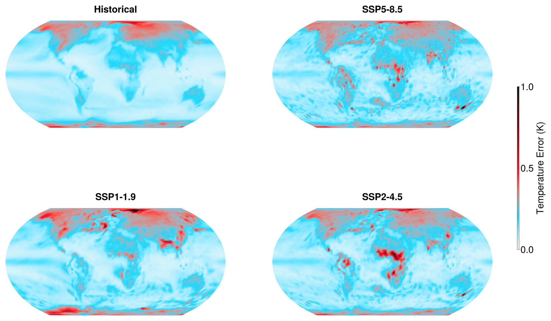
Figure 4 Absolute difference between pointwise emulated temperature and the ensemble mean from the MPI model averaged over all time for four different scenarios: the historical period (top left), SSP5-8.5 (top right), SSP1-1.9 (bottom left), and SSP2-4.5 (bottom right). The maximum temperature difference in the period 2015 to 2100 is 1.4 K for SSP5-8.5, 0.3 K for SSP1-1.9 and 1.4 K for SSP2-4.5. The emulator was trained on the historical period and SSP5-8.5; SSP2-4.5 and SSP1-1.9 are “test” scenarios.

5.1 Spatial Error

We begin by exploring the patterns of error in the emulator and comparing them across training and test scenarios. To understand the spatial distribution of error, we show in Fig. 4 the averaged absolute difference between our emulator-predicted mean temperature and the ensemble mean of the data over the historical period, SSP5-8.5, SSP2-4.5, and SSP1-1.9. In formulas, this is

$$\begin{array}{}\text{(18)}& \begin{array}{rl}\text{Error}\left(\mathit{x}\right)=& {\displaystyle \frac{\mathrm{1}}{\text{duration}}}\underset{\text{scenario start}}{\overset{\text{scenario end}}{\int }}\left|{\displaystyle \frac{\mathrm{1}}{\mathrm{12}}}\sum _m\right.\\ & \left.\times \left(\langle T(\mathit{x},m,t,\mathit{\omega })\rangle -\widehat{\mathit{\mu }}(\mathit{x},m,{\stackrel{\mathrm{‾}}{T}}_{\mathrm{g}}(t\left)\right)\right)\right|\mathrm{d}t\end{array}\end{array}$$

where 〈⋅〉 denotes an average over ensemble members ω. We have explicitly written down the dependence of the ESM temperature T on the month m, spatial location x, and year t and of the emulator estimate $\widehat{T}$ on the same variables, but with time t replaced with the appropriate global mean temperature ${\stackrel{\mathrm{‾}}{T}}_{\mathrm{g}}$ evaluated at the specified year. The integral is taken over a specified future scenario across all the years encompassed by that scenario.

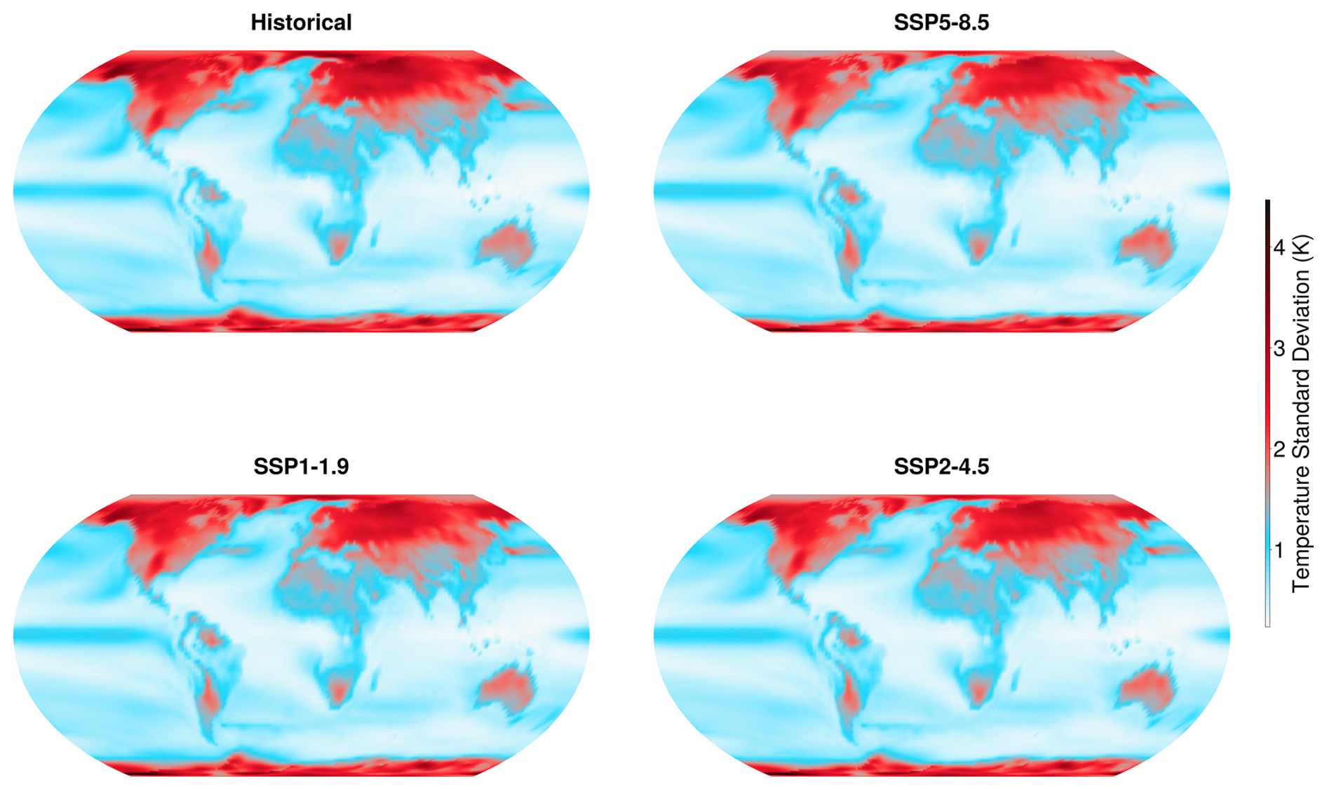
Figure 5 Pointwise standard deviation of surface temperature in the MPI model averaged over all months and over each scenario, laid out as in Fig. 4. The standard deviation is calculated across ensemble members for each time step. Note the high variability in the polar regions.

The emulator is quite accurate across the majority of the globe, especially when assessed relative to the internal variability of the system. For all scenarios, the largest errors are found in the high latitudes. There are also additional errors over Africa, India, and the southeast tip of Australia. Relative to the spatially varying temperature variability, however, only some of these errors are significant. Figure 5 illustrates the averaged pointwise standard deviation of surface temperature for each scenario shown in Fig. 4. The standard deviation is calculated across ensemble members, then averaged over time for each scenario. The variability of temperature is by far the largest in the polar regions; in these regions it is much larger than the errors of the emulator. Likewise, the errors over India and particularly the Himalayas coincide with regions of high temperature variance. Thus, when assessed relative to the internal variability of the ESM, the only significant emulation errors are those in equatorial Africa, in south-eastern Australia, and in the North Atlantic (for low-emissions scenarios).

Figure 6 Spatially coarse emulator statistics. The purple color indicates data coming from the MPI model over the historical training period with similar global mean temperatures, and in blue, the emulator prediction for the same period. The top panel shows the ensemble mean and variance of the zonally averaged January surface temperature field at each latitude, where the shading corresponds to three standard deviations. In the bottom panel, we show histograms at several fixed latitudes and compare the empirical distribution of the MPI data to the emulator prediction with an additional Gaussian assumption (for plotting purposes).

We expect the errors in spatial patterns to change upon using non-polynomial regression for the mean or a different set of basis functions. However, we argue against such an approach because we suspect that these errors reflect regional changes that depend on variables beyond global mean temperature, such as changes in dynamics due to the disappearance of sea ice in the Northern Hemisphere and changes in the hydrological cycle in the low latitudes. A more promising strategy would be to formulate an emulator that takes large-scale variables beyond the global mean temperature as input, but this is left for future work. For present purposes, we are encouraged by the fact that the spatial errors are largely consistent across all future scenario cases. This indicates that our emulator is effectively generalizing to scenarios for which it wasn't specifically trained.

In Appendix B we additionally explore the temporal error of the emulator and reconfirm that the emulator skill is improved significantly by our choice of using a quadratic, rather than linear, regression of EOF mean amplitudes on global mean temperature (Eq. 5). In Appendix C we report on the temporal error of the emulator's representation of temperature standard deviation. While these tests are commonly used in the assessment of emulators, they are limited in scope. In the next section, we illustrate a major advantage of our emulator: its ability to quantify the significance of shifts in the mean and variability of climate variables averaged over different spatial regions.

5.2 Spatial Statistics

As stated in Sect. 4.2, it is possible to reconstruct second-order spatial statistics of any observable of our system as long as it is a linear function of the variables we emulate. The statistics of the zonal average at a fixed latitude for temperature in January from the MPI model (purple) are reconstructed in Fig. 6 for a range of similar global mean temperatures taken over the historical period to have higher fidelity statistics. The corresponding predictions from the emulator are in blue. The emulator reconstructs very accurately the mean and variance for all latitudes (top row). In the bottom row, we compare the whole distributions of zonally averaged temperature at a few sample latitudes. Here, the emulated distributions are derived using the mean and covariances by assuming a multivariate Gaussian distribution for the EOF coefficients (see Appendix A for an extended discussion on Gaussianity). It is remarkable that such close agreement is achieved, given that the regression focuses on the mean and covariance of the EOF amplitudes rather than directly on the zonal averages. We emphasize, once again, that the emulator must predict the full covariance matrix for all EOF amplitudes–the main innovation of our work–to accurately capture the zonally averaged statistics of surface temperature at each latitude, as demonstrated in Eq. (17).

Figure 7 Distribution of temperature (top row) and relative humidity (bottom row) for the months of January (left) and July (right) for the years 1950 (historical scenario) and 2050 (SSP2-4.5 scenario) averaged over land and ocean. The emulator (solid line) captures the shift under climate change in the mean and variance of the data distributions (histograms). For plotting purposes, we use our emulator's mean and variance prediction as input to a Gaussian distribution.

Figure 8 Similar to Fig. 7, but for pointwise statistics at different locations on Earth rather than averaged over ocean and land. The emulator represents the overall trends in means and variances even when the distributions are non-Gaussian.

Until now, we have focused on surface temperature statistics, but applying the methodology to other variables is straightforward. As an example, we apply the method to surface relative humidity. We show the emulator prediction and the MPI data in Fig. 7 for two of the twelve months. We show the probability distributions of surface temperature (top row) and relative humidity (bottom row) averaged over land and ocean separately, where, to visualize the emulator estimates, we have assumed a multivariate Gaussian form for the distributions. We re-emphasize that the assumption of Gaussianity is only necessary for generating full distributions, but the emulation of means and covariances remains valid even for variables with non-Gaussian statistics. For example, our emulator can be used to emulate the mean and covariance of pointwise precipitation, but a Gaussian approximation would fail to reproduce its full distribution, which is known to depart strongly from Gaussian. Here, we compare the temperature and relative humidity distributions for the years 1850 and 2050, where the latter is taken from the SSP2-4.5 scenario. While this scenario was not used in training, the emulator prediction for 2050 closely matches the MPI data. This further supports the generalizability of the emulator to arbitrary future scenarios. See Fig. D2 in Appendix D for the same statistics as Fig. 7 but for the SSP5-8.5 training scenario. Inspection of probability distributions can be used to determine whether the shifts in the mean values of temperature and relative humidity over this century are significant or not. For temperature, we see that the distribution shifts towards a warmer climate are outside of the internal variability. For relative humidity, the shifts in its mean value are in accordance with the expectation that relative humidity will decrease over land in a warmer climate and increase over the ocean (Byrne and O'Gorman, 2016). However, the distributions shows that these shifts in mean relative humidity are outside of the internal variability in July, but not in January.

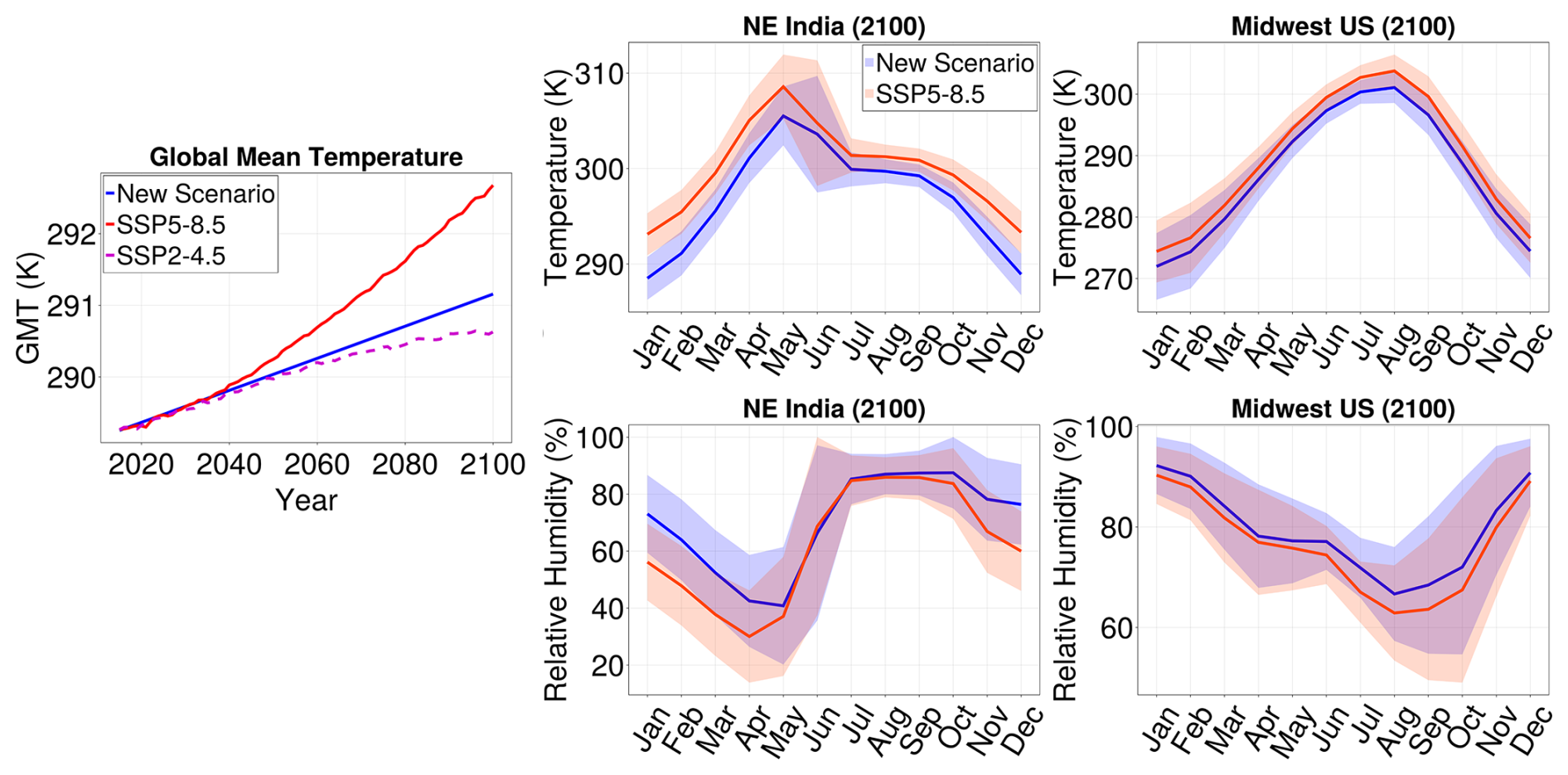
Figure 9 Case study: Using the emulator to assess regional impacts of emissions reduction. On the left, we define a new scenario (blue) in the global mean temperature. In the second and third columns, ribbon plots show monthly mean temperature (top) and relative humidity (bottom) ± 2σ in 2100 in SSP5-8.5 (red) and the new scenario (blue) for two locations: NE India and Midwest US. This illustrates the importance of internal variability in climate assessment.

Having shown that our emulator both captures spatial statistics and generalizes to previously unseen future scenarios, we proceed to illustrate how it might be used in practice. Figure 8 repeats the analysis of Fig. 7 but for pointwise statistics at two locations. We can use the emulator to observe the localized effects of climate change under SSP2-4.5. We see apparent shifts in the pointwise temperature distributions (top row), but less so for relative humidity (bottom row), where in all cases, the shifts in mean are well within the internal variability (variance). The relative heights of the distributions within a given panel offer a quick way to assess whether the variance has shifted. For example, there seems to be an increase in variance in the top left panel, and a decrease in variance in the top right panel. For both temperature and relative humidity, we see that shifts of means and variances are well captured. We re-emphasize that our emulator produces means and covariances which, for convenience, we plot as Gaussian distributions. Even in cases where the underlying distribution is non-Gaussian, the emulator captures the evident trends in mean and variance. Overall, the pointwise variance is well-represented by our model; see Fig. C2 in Appendix C for a quantitative metric. The following section further illustrates how the emulator can be used to study an arbitrary warming scenario outside of the SSP framework.

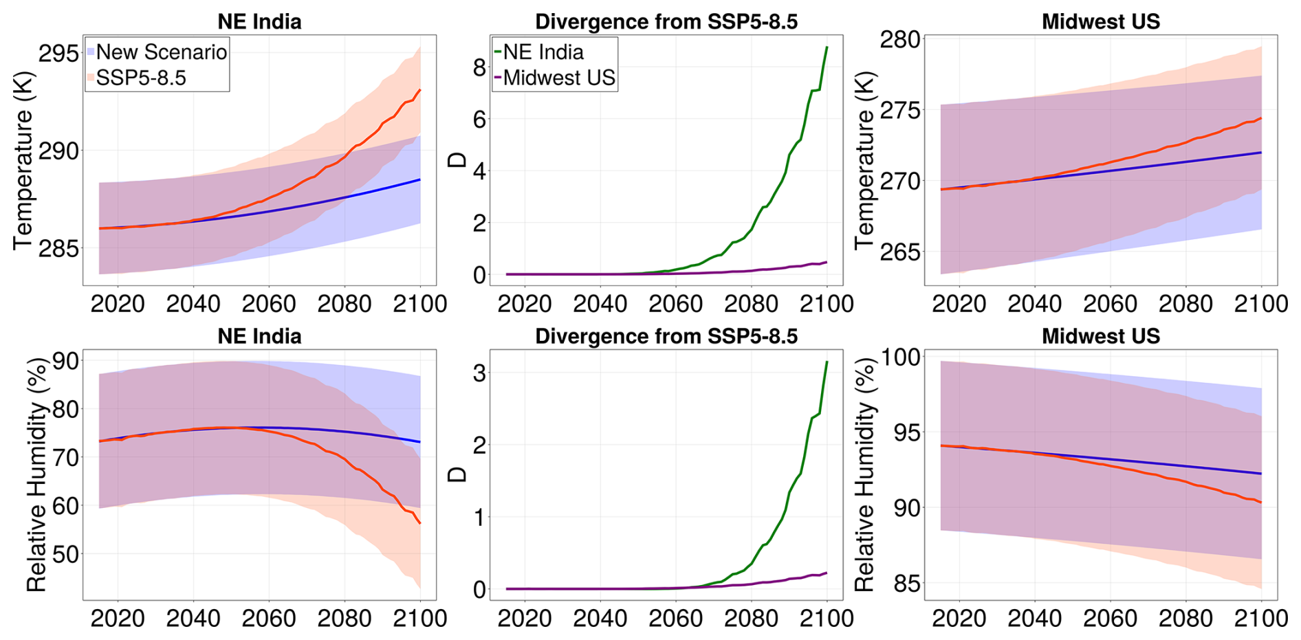
Figure 10 Case study: time of emergence. All panels are for the month of January. First and third columns show evolution of January values of monthly average temperature (top) and relative humidity (bottom) in NE India (left) and Midwest US (right) under the SSP5-8.5 scenario (red) and the new scenario (blue). The bands correspond to 2 standard deviations from the mean, computed over the region. The second column illustrates, for the new scenario, the KL divergence from SSP5-8.5 of the January distribution of monthly mean temperature (top) and relative humidity (bottom) over time in both locations.

6 Emulator Usage and Case Study

Thus far, we have only applied the emulator to reproduce SSP scenarios to test its skill in generalizing to scenarios not used in the training. In practice, however, the main application of an emulator is in quickly and cheaply inferring the behavior of an ESM in arbitrary scenarios. Figures 9 and10 illustrate a case study for such an application, motivated by the idea of the time of emergence (ToE) of a climate signal. We define an arbitrary new climate change scenario in terms of the global mean temperature. This scenario, which is shown in the first column of Fig. 9, grows exponentially at a rate significantly slower than that of SSP5-8.5, with an end-of-century global mean temperature 3 °C above the 1850–1900 average. One could imagine that this scenario is the result of a slight reduction of emissions, driven by changing economic incentives, but without strong international cooperation on climate goals. If we follow the course set out by this scenario, how soon would we be able to see the effects of emission reduction relative to the worst-case path of SSP5-8.5? In other words, when will the diverging scenarios yield significantly different climate statistics, and how will this vary across different locations on Earth? Questions such as these are relevant as they can help quantify the regional impact of climate policy over time. Similar questions have been explored in the BRACE project (O'Neill et al., 2018), but focusing only on two pre-defined scenarios.

To answer these questions, we examine the statistics for temperature and relative humidity at two geographic locations: (40.1° N, 88.1° W) in the Midwest United States, near Chicago, and (23.3° N, 84.4° E) in Jharkand, in northeastern India. Each region spans four cells on the ESM numerical grid. In the second and third columns of Fig. 9 we show the respective distributions of temperature (top) and relative humidity (bottom) at the end of the century (in 2100) for all months. We plot, for both SSP5-8.5 and the new scenario, the mean monthly values ± 2 standard deviations as estimated by the emulator. For both locations, the variance provides critical context for assessing whether a change in mean is significant. Note that, for both variables, the difference between the two scenarios is much more prominent in NE India. In contrast, in the Midwest US, the differences between the scenarios are largely within the range of internal variability of the model; e.g., although the mean relative humidity in August appears to change, accounting for variance suggests that this change is not statistically significant. The emulator additionally resolves the impact of the two scenarios by seasons; e.g., for relative humidity in NE India, there is a significant difference between the scenarios only in the winter months November-April. It would be impossible to resolve such nuances without the emulated covariances, which allow us to calculate the standard deviations of variables over arbitrarily sized regions.

Our emulator can further be used to quantify how soon the effects of a reduction in emissions will be felt, which we illustrate in Fig. 10. The left and right columns of Fig. 10 show, for NE India and the Midwest US, respectively, the evolution of projected January mean temperature (top) and relative humidity (bottom) under SSP5-8.5 (in red) and the new scenario defined in Fig. 9 (in blue). The bands correspond to ± 2σ over the regions, as projected by the emulator. The figure illustrates that towards the end of the century, the two scenarios begin to significantly diverge beyond what is naturally expected from the local climate variability in NE India, but not in the Midwest US. We might consider the time when one observes a divergence beyond natural variability as the time of emergence of the effects of climate mitigation in the new scenario. In the middle column, we quantify this notion using the Kullback-Leibler divergence, which we proceed to describe below.

We are interested in the change over time (under a particular climate change scenario) of some distribution d₁ of a climate variable, computed over a region of interest. In particular, we would like to measure the difference between this distribution in the given scenario and the same distribution d₂ in a reference scenario (e.g., business-as-usual, or SSP5-8.5). At which point in the future would we be able to say that the two scenarios are significantly different? This question is essentially a generalization of the question of the ToE of a climate change signal. To answer it, one might look at when the mean of d₁ is one or two standard deviations away from the mean of d₂. We instead use the Kullback-Leibler (KL) divergence to quantify at every point in time the difference between the two distributions. The KL divergence is a widely used information-theoretic measure related to Shannon entropy (Shlens, 2014; Geogdzhayev et al., 2024). For two general continuous distributions P and Q, the KL divergence D is defined as

$$\begin{array}{}\text{(19)}& D(P,Q)=\underset{-\mathrm{\infty }}{\overset{\mathrm{\infty }}{\int }}p\left(x\right)\log \left({\displaystyle \frac{p\left(x\right)}{q\left(x\right)}}\right)\mathrm{d}x.\end{array}$$

In order to apply the divergence to our case study, we thus must assume a form of the distribution parameterized by the means and covariances given by the emulator. Following the plotting convention adopted throughout this work, we assume a Gaussian form for the distributions. For two Gaussian distributions d₁ and d₂, the KL divergence simplifies to

$$\begin{array}{}\text{(20)}& D(d_{\mathrm{1}},d_{\mathrm{2}})=\ln \left({\displaystyle \frac{{\mathit{\sigma }}_{\mathrm{2}}}{{\mathit{\sigma }}_{\mathrm{1}}}}\right)+{\displaystyle \frac{{\mathit{\sigma }}_{\mathrm{1}}^{\mathrm{2}}+({\mathit{\mu }}_{\mathrm{1}}-{\mathit{\mu }}_{\mathrm{2}}{)}^{\mathrm{2}}}{\mathrm{2}{\mathit{\sigma }}_{\mathrm{2}}^{\mathrm{2}}}}-{\displaystyle \frac{\mathrm{1}}{\mathrm{2}}}\end{array}$$

where $d_{\mathrm{1}}\sim \mathcal{N}({\mathit{\mu }}_{\mathrm{1}},{\mathit{\sigma }}_{\mathrm{1}}^{\mathrm{2}})$ and $d_{\mathrm{2}}\sim \mathcal{N}({\mathit{\mu }}_{\mathrm{2}},{\mathit{\sigma }}_{\mathrm{2}}^{\mathrm{2}})$. Note that the KL divergence is an asymmetric measure, and Eq. (20) quantifies the divergence of d₁ from d₂. Although D is dimensionless, one can use 0.5 and 2 as approximate benchmarks for 1σ and 2σ significance, respectively. We obtain these values by setting σ₁=σ₂ and ${\mathit{\mu }}_{\mathrm{1}}={\mathit{\mu }}_{\mathrm{2}}-{\mathit{\sigma }}_{\mathrm{2}}$ to yield D=0.5. Similarly, setting σ₁=σ₂ and ${\mathit{\mu }}_{\mathrm{1}}={\mathit{\mu }}_{\mathrm{2}}-\mathrm{2}{\mathit{\sigma }}_{\mathrm{2}}$ yields D=2.

The middle column in Fig. 10 shows, for both locations, the time evolution of the KL divergence between the new scenario and SSP-8.5 distributions for the January surface temperature (top) and relative humidity (bottom). In both locations, the temperature differences between scenarios are more significant than the relative humidity ones. For both temperature and relative humidity, the effects of the emission reduction would be more significantly felt in NE India, as evidenced by higher values of D, in agreement with visual assessment of the distributions. These effects would also be felt sooner: if we consider D=0.5 to be the approximate significance threshold for a 1σ change, a significant change in NE India would be felt by 2068, while in the Midwest US it would still not be approached by 2010 when the divergence reaches a maximum value of D=0.44. The same is true for relative humidity: in NE India, the effect of emissions reduction on relative humidity would be felt both sooner and more significantly. We would observe a significant change around 2080 in NE India, and not before the end of the century for the Midwest US, with a maximum end-of-century value of D=0.22.

In this case study, we have demonstrated how our emulator may be used to assess the effects of a reduction in emissions on regional climate outcomes. In a similar vein, our emulator could also be used to assess the ToE of a particular climate signal by comparing a possible future scenario with a baseline no-warming scenario. Our emulator is well-suited to such policy and impact assessment problems. The modeling of EOF covariances allows for the seamless calculation of variances across spatial scales, providing crucial information to quantify significance and uncertainty. Furthermore, our model is lightweight and computationally efficient, meaning it can be run almost instantaneously to iterate on different scenarios. These two features make it an ideal tool for policymakers, educators, and scientists looking to quickly explore outcomes of widely varying future climates.

7 Conclusions

We have introduced an emulator for the evolution of the means and covariances of climate variables and applied it to spatially resolved monthly averaged temperature and relative humidity. This emulator provides a simple and computationally efficient method for extending the MPI-ESM1.2-LR global climate model to arbitrary warming scenarios while retaining the ability to quantify the significance of trends by modeling covariances. Computational efficiency is achieved by limiting the emulation to means and covariances and by compressing the data onto the leading 1000 EOF modes of variability, reducing its memory footprint by two orders of magnitude compared to the training dataset. This dimensionality reduction is not a significant limitation, as Earth System Models have substantially greater fidelity at large scales than at fine spatial resolution.

We have focused on accurately capturing the internal variability of the original ESM and flexibly generalizing it to previously unseen warming scenarios. The internal variability provides critical context for the assessment of projected changes in the climate. Thanks to our modeling of the full EOF covariance structure, the design of our emulator allows for the seamless calculation of second-order statistics across regions of any size, allowing for easy calculation of regional-scale variability. We assume that EOF covariances vary smoothly with global mean surface temperature. However, this assumption may break down in regions or timescales where localized processes – such as abrupt sea ice loss or monsoon regime shifts – introduce discontinuities in the covariance structure. Capturing such transitions may require future extensions that incorporate non-smooth, regime-dependent components.

Several straightforward extensions of the proposed emulator are possible. These include applying the method to additional climate fields, adopting alternative basis functions, using higher-order regression schemes, or incorporating additional predictors beyond global mean temperature. The framework can also be used to capture correlations between different variables (e.g., temperature and relative humidity) by modeling joint EOF amplitudes or post hoc correlations. Temporal coherence could similarly be introduced, for example, by estimating auto-covariances of EOF amplitudes across months.

The emulator framework we introduced cannot be easily extended to statistics beyond means and covariances. Estimating even the three-point correlation of a high-dimensional distribution becomes cumbersome, requiring the computation and storage of a tensor with N³ points if one uses a basis of N EOF amplitudes. Generally, a multivariate distribution of size N necessitates the storage of Nⁿ points for an n-point correlation, rapidly becoming intractable for large N or n. To emulate higher-order statistics, like weather extremes, generative models like diffusion-based emulators (Song et al., 2020; Bouabid et al., 2025) may be better suited. These approaches are well-equipped to capture higher-order correlations. However, this added flexibility comes with increased cost and training requirements, which may limit its use in applications that demand fast inference and interpretability on limited hardware. Our emulator is, on the other hand, well suited for computation-limited applications.

More generally, the present work lays the foundation for specialized downstream emulators. For example, one could condition a high-resolution or extreme-event emulator on monthly temperature fields produced by our framework. This would integrate well with existing techniques, including Generalized Extreme Value theory or machine-learning-based generative models. Recent work, such as Bassetti et al. (2024) and Christensen et al. (2024) illustrates how such hybrid frameworks might be developed. Figure 11 sketches a potential ecosystem of interconnected emulators. A simple climate model (e.g., FaIR-GP, Bouabid et al., 2024) translates emissions scenarios into global mean temperature trajectories. These are passed to an emulator of monthly-averaged spatial fields such as the one developed here. The final stage would use a downscaling model to reconstruct finer-grained or daily fields. For example, the DiffESM emulator (Bassetti et al., 2024) uses monthly climate values as input to generate daily values; an ensemble of different values, which can be generated with out probabilistic emulator, can be used to condition different daily outcomes. Limitations of this pipeline framework include the assumption that all regional statistics are determined by the global mean surface temperature and the challenge of capturing spatially heterogeneous forcing agents such as aerosols.

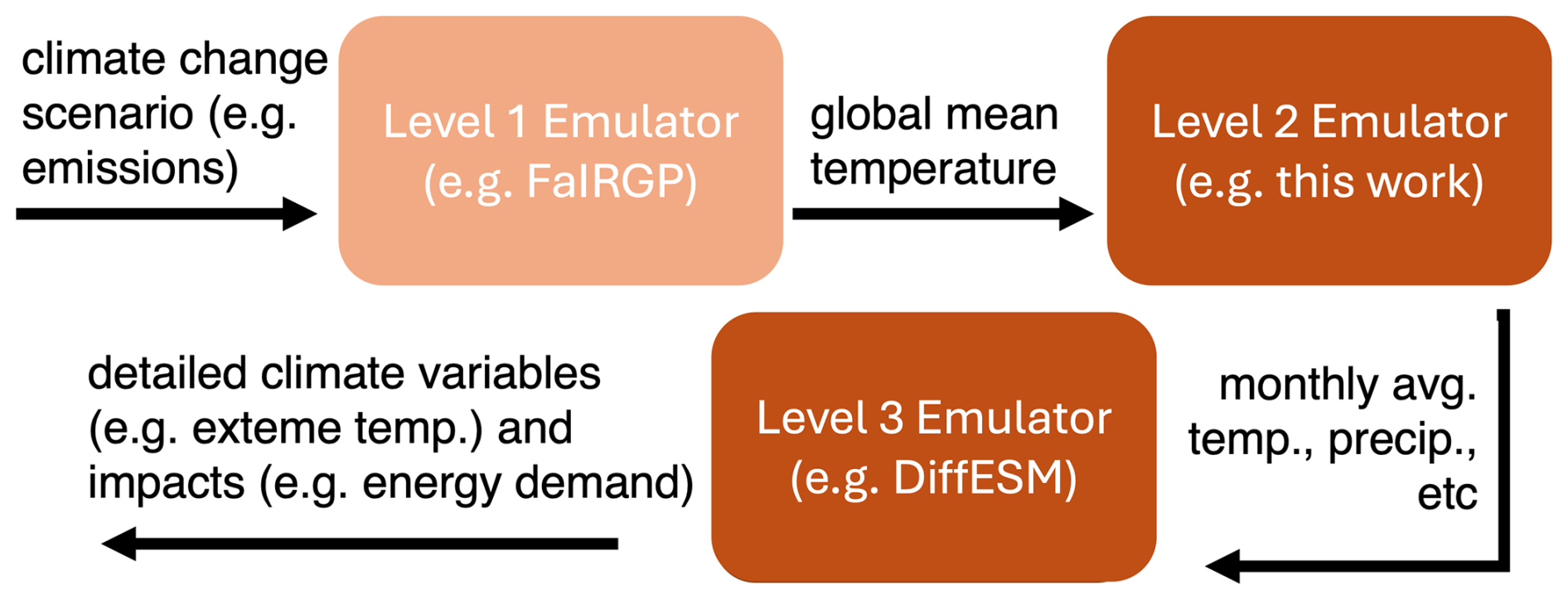
Figure 11 Potential ecosystem for coupled emulator models. FairGP (Bouabid et al., 2024) is an example of a simple climate model (SCM) that translates emissions scenarios to global mean temperature. DiffESM (Bassetti et al., 2024) is an example of a model that emulates daily values of climate fields conditioned on monthly mean temperature.

Projections accounting for model spread, such as those emulated in this work, are vital to designing effective solutions to climate adaptation (Hansen et al., 2012; Deser et al., 2012; Woodruff, 2016). The low computational cost of our emulator makes it well suited for applications that benefit from quick iteration on the warming scenario being explored, such as policy and economic analysis, climate communication, and education. Once trained, our emulator can be run many times at little additional cost on modest hardware such as single-core CPUs. We have experimented with using the emulator in a prototype graphical climate education tool that visualizes changes in regional climate impacts from various warming mitigation policies. While the present emulator is trained on a particular Earth System Model (MPI-ESM1.2-LR), the methodology is broadly applicable to any model ensemble with sufficient realizations. Moreover, such model-trained emulators can serve as physically consistent priors that are further constrained with observational data to reduce structural model bias, as demonstrated in Immorlano et al. (2025).

Appendix A: Statistics of EOF Amplitudes and Pointwise Quantities

We mention in Sect. 3 that under certain assumptions, it is possible to translate the means and covariances produced by our emulator into higher-order statistics. For example, leading EOFs represent averages of the original variables over large swaths of Earth and, as such, are generally well-represented as multivariate Gaussians from central limit theorem arguments. Both monthly and spatial averaging make the multivariate statistics of the EOF amplitudes more Gaussian than the original variables. To substantiate this ansatz, we leverage evidence from the literature that spatially coarse-grained and monthly mean temperatures follow a Gaussian distribution (e.g., Schär et al., 2004; Hansen et al., 2010; Schneider et al., 2015; Falasca et al., 2025, 2024). The multivariate Gaussian assumption is more appropriate for smoothly varying variables like temperature and relative humidity than for variables like precipitation, which have a much more nonlinear response to temperature fluctuations and non-Gaussian statistics (Legates, 1991).

Although not necessary for the work in the main text, we will show that we can represent many statistics of interest by assuming that a_C is well represented by a multivariate Gaussian, i.e.

$$\begin{array}{}\text{(A1)}& \mathit{\rho }\left({\mathit{a}}_{\mathrm{C}}|{\stackrel{\mathrm{‾}}{T}}_{\mathrm{g}},m\right)\approx \mathcal{N}\left(\mathit{\mu }\left({\stackrel{\mathrm{‾}}{T}}_{\mathrm{g}},m\right),\mathcal{C}\left({\stackrel{\mathrm{‾}}{T}}_{\mathrm{g}},m\right)\right),\end{array}$$

where the coarse statistical variables a_C are approximated as a Gaussian distribution, denoted 𝒩, with means μ and covariances 𝓒 as a function of the global mean temperature ${\stackrel{\mathrm{‾}}{T}}_{\mathrm{g}}$ and month m.

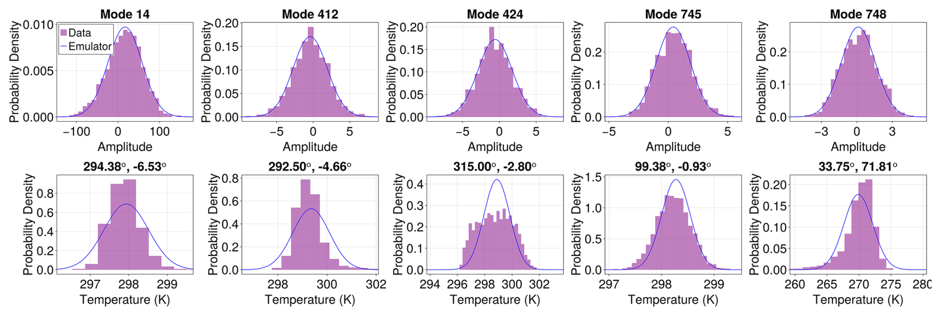
Figure A1 Statistics of surface temperature EOF modes and selected locations. In purple, we show the histograms of data collected over the historical period of the MPI ensemble with similar global mean temperatures. In blue, we show the fit given by the emulator described in this work. The EOF amplitudes populate the top row, and the bottom row constitutes point locations. The locations and modes were selected for being the least Gaussian, except for Mode 412 and location 99.39°, −0.93° which are the most Gaussian.

For example, we show in Fig. A1 the distributions of EOF modes at selected locations of surface temperature in purple, chosen from a subset of the historical period of the MPI ensemble with similar global mean temperatures. The figure illustrates the four most “non-Gaussian” modes/locations and one “most Gaussian” mode/location. Specifically, the modes and locations were selected by constructing histograms for every location and mode, finding the locations/modes with the most positive/negative kurtosis and skewness (four total) and one location with skewness and kurtosis closest to zero. We show in blue the result of the emulator mean and variance prediction for the statistics under a Gaussian assumption.

We see from Fig. A1 that even the most “non-Gaussian” EOF coefficients (top row) display a familiar bell-shaped curve, whereas the different locations for pointwise statistics display non-Gaussian features (bottom row). A subtle point now arises. All distributions of the EOF coefficients appear to be quasi-Gaussian. Furthermore, point statistics can be reconstructed from the EOF mode statistics and the EOF basis through a linear sum. Lastly, sums of Gaussian random variables are Gaussian. Reconciling these three facts with the non-Gaussian point statistics of the bottom row in Fig. A1 requires non-Gaussian higher-order correlations between the different EOF modes. These non-Gaussian correlations ought to be captured to emulate the tails of the distributions at a location; this could be achieved with other data-driven methods such as “score-matching” or Markov models (see Souza, 2024a, b; Giorgini et al., 2024; Bassetti et al., 2024; Christensen et al., 2024). In this work, we focus on robust spatially coarse-grained and lower-order statistics. This focus allows us to ignore these higher-order moment effects.

Appendix B: Linear emulator

In constructing our emulator we used a quadratic function to regress the mean EOF coefficients onto ${\stackrel{\mathrm{‾}}{T}}_{\mathrm{g}}$, see Eq. (5). However, we also experimented with using a linear function to perform the same regression:

$$\begin{array}{}\text{(B1)}& \widehat{\mathit{\mu }}={\widehat{\mathit{\mu }}}_{\mathrm{0}}+{\widehat{\mathit{\mu }}}_{\mathrm{1}}{\stackrel{\mathrm{‾}}{T}}_{\mathrm{g}}.\end{array}$$

We found the linear emulator to result in a slightly worse fit, which we illustrate in Fig. B1. In the top row of Fig. B1, we plot the difference in the yearly and ensemble-averaged global temperature emulation error between the linear and quadratic emulators as a function of time. Emulators using an increasing number of EOF modes (10, 100, 1000) are plotted in different colors. At each time along the horizontal axis, the errors for both emulators are computed with respect to ${\stackrel{\mathrm{‾}}{T}}_{\mathrm{g}}$ from the MPI ensemble for the year in question; the error of the quadratic emulator is then subtracted from that of the linear emulator. In formulas, we are comparing (for each year) between the two emulators

$$\begin{array}{}\text{(B2)}& \begin{array}{rl}& \text{temporal\hspace{0.17em}\hspace{0.17em}error}(T,\widehat{T})=\\ & \sqrt{{\displaystyle \frac{\mathrm{1}}{\mathrm{4}\mathit{\pi }}}\underset{\mathit{\theta }=\mathrm{0}}{\overset{\mathrm{2}\mathit{\pi }}{\int }}\underset{\mathit{\varphi }=\mathrm{0}}{\overset{\mathit{\pi }}{\int }}\begin{array}{c}|\frac{\mathrm{1}}{\mathrm{12}}\sum _m\left(\langle T(\mathit{x},m,t,\mathit{\omega })\rangle -\widehat{\mathit{\mu }}\left(\mathit{x},m,{\stackrel{\mathrm{‾}}{T}}_{\mathrm{g}}\left(t\right)\right)\right){|}^{\mathrm{2}}\\ \times \sin \left(\mathit{\varphi }\right)d\mathit{\theta }d\mathit{\varphi }\end{array}},\end{array}\end{array}$$

where 〈⋅〉 to denotes an ensemble average. The spatial average is taken over the surface of Earth, with $\mathit{x}=(\mathit{\theta },\mathit{\varphi })$, and t here denotes a fixed year. We emphasize that the training for both emulators is performed on the historical period and SSP5-8.5, whereas our “test” is with respect to SSP1-1.9 and SSP2-4.5.

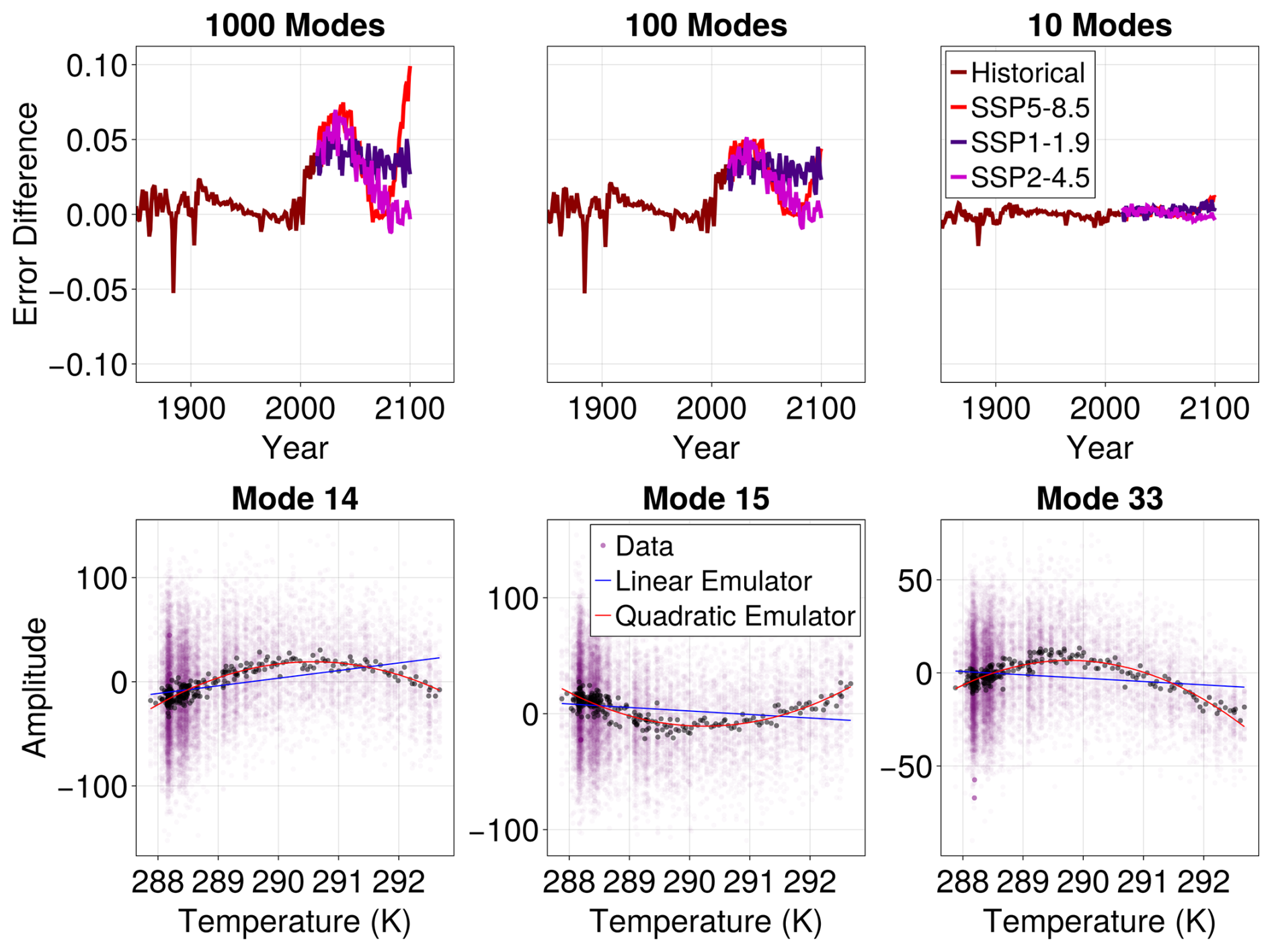
Figure B1 Difference in regression error between linear and quadratic emulators. Top row: difference in regression (emulation) error for ensemble and yearly averaged surface temperature as a function of time for different scenarios. Error of the quadratic emulator is subtracted from that of the linear emulator, so positive values indicate higher error in the linear emulator. Bottom row: fit comparison between quadratic and linear emulators for the three “most quadratic” EOF modes, analogous to Fig. 3.

Note that for a small number of modes, the linear and quadratic emulators perform about the same. As we increase the number of modes, however, the quadratic emulator has significantly lower errors in future scenarios where nonlinear effects become more prominent. The only significant exception is the historical period, in which the quadratic emulator appears to overfit to large volcanic events. The bottom row of Fig. B1 illustrates the origin of the improvement in fit yielded by the quadratic emulator. Here we repeat the plots in Fig. 3 for the three “most quadratic” modes (where the regression error difference between the linear and quadratic fit was maximal). The EOF coefficients of these modes – and many others – have a distinct quadratic dependence on ${\stackrel{\mathrm{‾}}{T}}_{\mathrm{g}}$, which is not captured by a linear emulator.

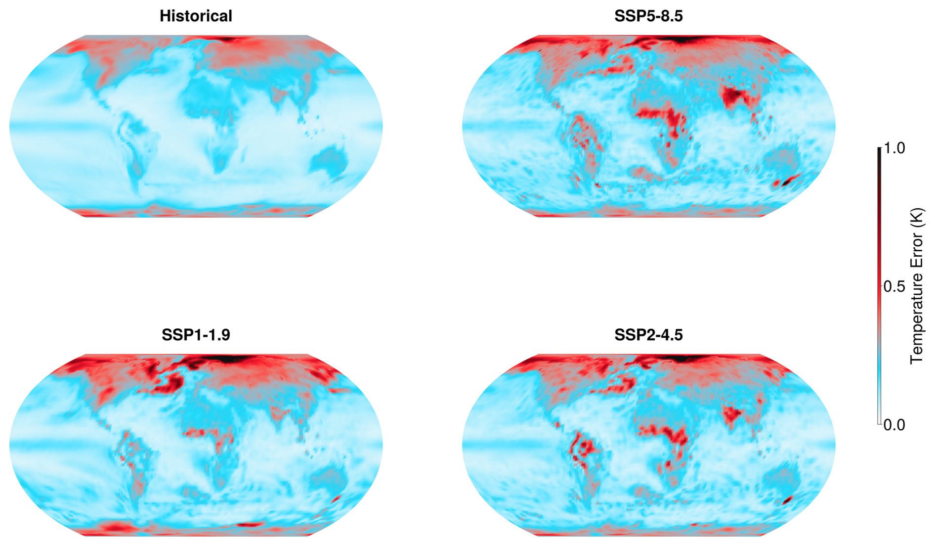
Figure B2 Average regression error of a linear emulator for ensemble and yearly averaged surface temperature as a function of space for different scenarios. Same as Fig. 4, but for a linear emulator instead of a quadratic one.

We additionally compare the spatial error, as defined in Eq. (18), of the linear and quadratic emulators. Figure B2 shows the same spatial errors over the different scenarios as Fig. 4, but for the linear emulator. Comparing the two figures, one observes a significant reduction in errors for the quadratic emulator, most notably in the Arctic, the North Atlantic, South Asia, and Sub-Saharan Africa.

Appendix C: Comparison to linear pattern scaling

To demonstrate that the linear version of our emulator, as described above in Appendix B, reduces to a form of a linear pattern scaling emulator for mean temperature at a single location, we plot in Fig. C1 the temporal error defined in Eq. (B2) as a function of time for an increasing number of EOF modes used in the emulator (10, 100, 1000). We compare the error of performing linear regression pointwise (i.e. applying pattern scaling) on the ensemble mean in the historical period and SSP5-8.5 to the error of the mean generated by our linear emulator. We re-emphasize that the training for both emulators is performed on the historical period and SSP5-8.5, whereas our “test” is with respect to SSP1-1.9 and SSP2-4.5.

As we increase the number of modes, the error in the approximation becomes similar to the pointwise error when utilizing pattern scaling. In the limit of using all EOF modes, we expect this error to match that of pattern scaling. This is to be expected: a few modes corresponding to large-scale patterns cannot represent the ensemble mean's spatial structure in scenarios outside the historical period. This error is due to a combination of two factors. The basis functions are constructed over the historical period, and secondly, even though we fit to SSP5-8.5 data for the EOF amplitudes, there is less data corresponding to warmer temperatures. Thus, the emulator underperforms when it sees less data. With more modes (and hence a more complete basis for representing functions), we see that the generalization error of going to different SSP scenarios matches the error of the historical period. Additionally, the quadratic version of the emulator described in the main text improves upon the errors shown in Fig. C1, see Fig. B1. We illustrate the error of the linear emulator here for the sake of an accurate comparison with pattern scaling.

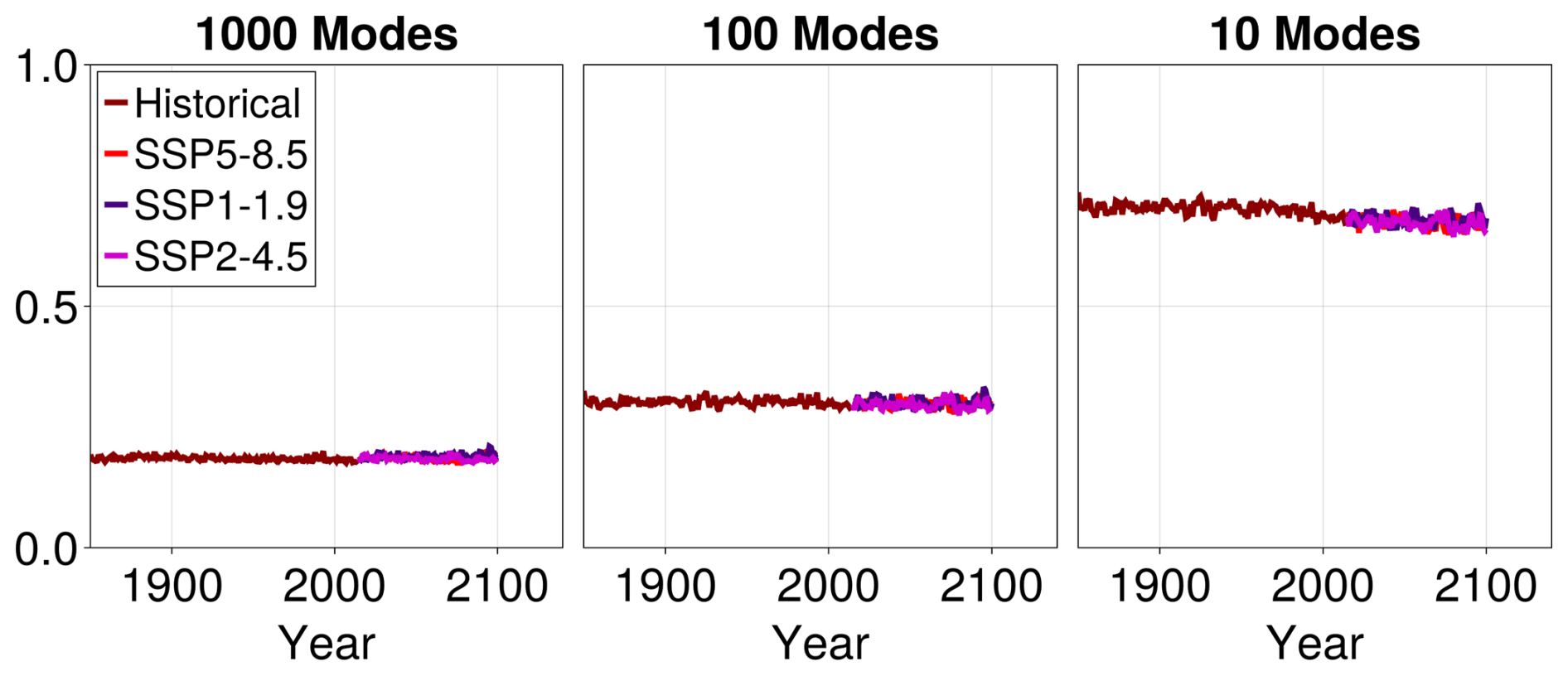
As discussed in the main text, a major advantage of our emulator over a method like pattern scaling is the direct emulation of covariances. To help illustrate this, we additionally plot in Fig. C2 the temporal error of the ensemble-averaged standard deviation of January surface temperature as a function of time and for an increasing number of modes. In formulas, this is analogous to Eq. (B2):

$$\begin{array}{}\text{(C1)}& \begin{array}{rl}& \text{Temporal\hspace{0.17em}\hspace{0.17em}Error }({\mathit{\sigma }}_{T,m},{\widehat{\mathit{\sigma }}}_{T,m})=\\ & \sqrt{{\displaystyle \frac{\mathrm{1}}{\mathrm{4}\mathit{\pi }}}\underset{\mathit{\theta }=\mathrm{0}}{\overset{\mathrm{2}\mathit{\pi }}{\int }}\underset{\mathit{\varphi }=\mathrm{0}}{\overset{\mathit{\pi }}{\int }}|{\mathit{\sigma }}_{T,m}-{\widehat{\mathit{\sigma }}}_{T,m}{|}^{\mathrm{2}}\sin (\mathit{\varphi })d\mathit{\theta }d\mathit{\varphi }}.\end{array}\end{array}$$

For a given number of modes, the standard deviation errors are approximately constant as a function of time. This illustrates that almost the entirety of the emulator's error in representing variance comes from the EOF approximation. Accordingly, as the number of EOF modes included increases, the error decreases.

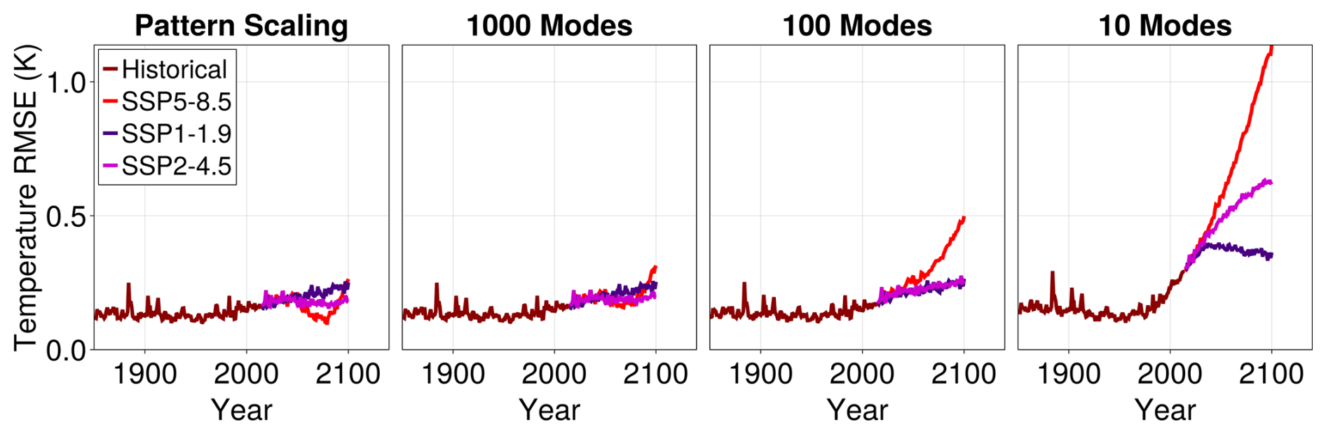
Figure C1 Regression error for ensemble and yearly averaged surface temperature as a function of time for different scenarios for a linear emulator. Different colors correspond to the historical 1850–2014 period (maroon) and the three future scenarios considered in this study: SSP5-8.5 (red), SSP2-4.5 (pink), and SSP1-1.9 (purple). The future period spans 2015–2100. The historical period lasts 165 years, and the projected period – 86 years. We show the root mean square error of pattern-scaling on the left and increasing the number of modes used in the linear emulator in the subsequent rightward panels. As we increase the number of modes, the error in capturing pointwise statistics decreases.

Figure C2 Regression error for ensemble averaged January surface temperature standard deviation as a function of time for different scenarios. Same as last three panels of Fig. C1, but for the standard deviation of temperature in January.

Appendix D: Extended validation

In this appendix we provide additional figures in support of the validation of our emulator design, see Sect. 5 in the main text.

Since our emulator captures each month separately, we can investigate a-posteriori shifts in the ensemble average seasonal temperature cycle. In Fig. D1, we show the seasonal emulator prediction for the Northern and Southern Hemisphere averages separately, where the blue corresponds to a global mean temperature in the historical period and the orange corresponds to the end of the SSP5-8.5 scenario. The amplitude of seasonal variation changes by approximately one Kelvin in the Northern Hemisphere and is smaller in the Southern Hemisphere. This asymmetry reflects the larger fraction of land in the Northern Hemisphere (land warms more than the ocean because it is drier and less efficient at cooling through latent heat release).

Additionally, Figs. D2 and D3 show the same statistics as Figs. 7 and 8, respectively, but for the training scenario SSP5-8.5.

Finally, Figs. D4 and D5 illustrate, for surface temperature, the differences between the emulator and the original MPI data in 2100 across the three future scenarios. Figure D4 shows the year-average mean surface temperature, while Fig. D5 shows the standard deviation of surface temperature in January. These spatial patterns are similar between the emulator and the data.

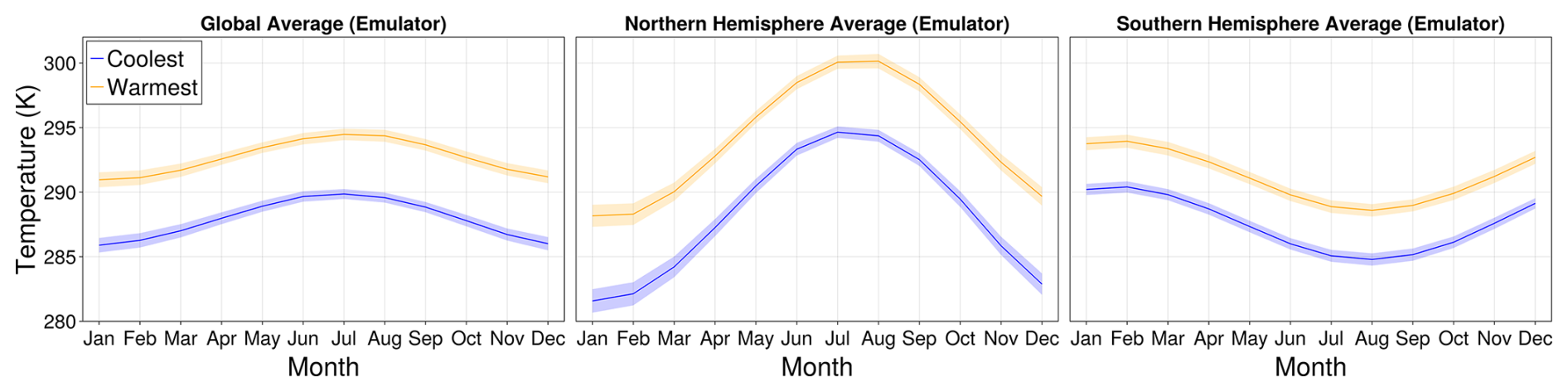
Figure D1 Monthly emulator output for global quantities. We show the emulator prediction for the global average (left), Northern Hemisphere average (middle), and Southern Hemisphere average (right), as well as two global mean temperatures, ${\stackrel{\mathrm{‾}}{T}}_{\mathrm{g}}$ = 288  (K) (blue) and ${\stackrel{\mathrm{‾}}{T}}_{\mathrm{g}}$ = 293  (K) (orange). The solid line indicates the ensemble average, and the shaded region indicates three standard deviations. We see a shift in the seasonal cycle for a warmer climate. In particular, in the past Northern Hemisphere, January has become similar to April.

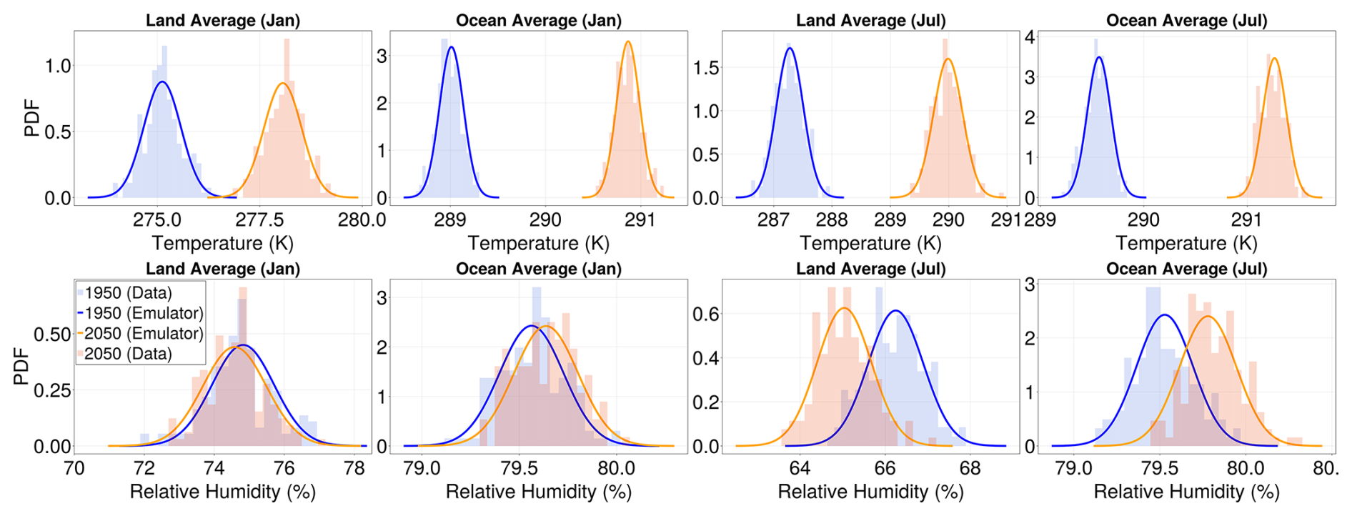
Figure D2 Distributional shifts under climate change for land and ocean spatial averages in SSP5-8.5. Same as Fig. 7, but here we compare the historical and SSP5-8.5 scenarios.

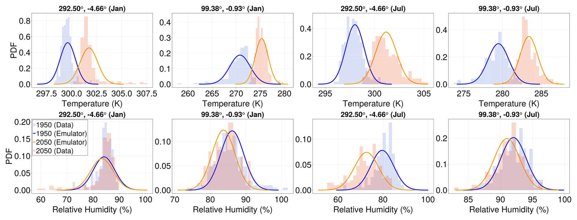
Figure D3 Distributional shifts under climate change for different locations in SSP5-8.5. Same as Fig. 8, but here we compare the historical and SSP5-8.5 scenarios.

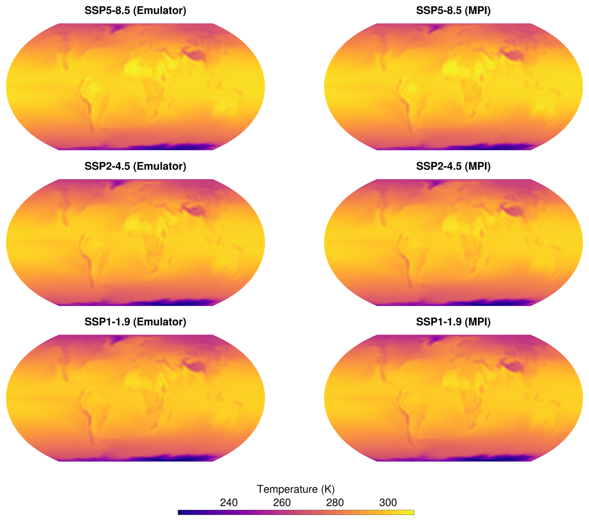
Figure D4 Emulator representation of yearly-average mean surface temperature in 2100. Emulator representation on the left, MPI model data on the right for comparison.

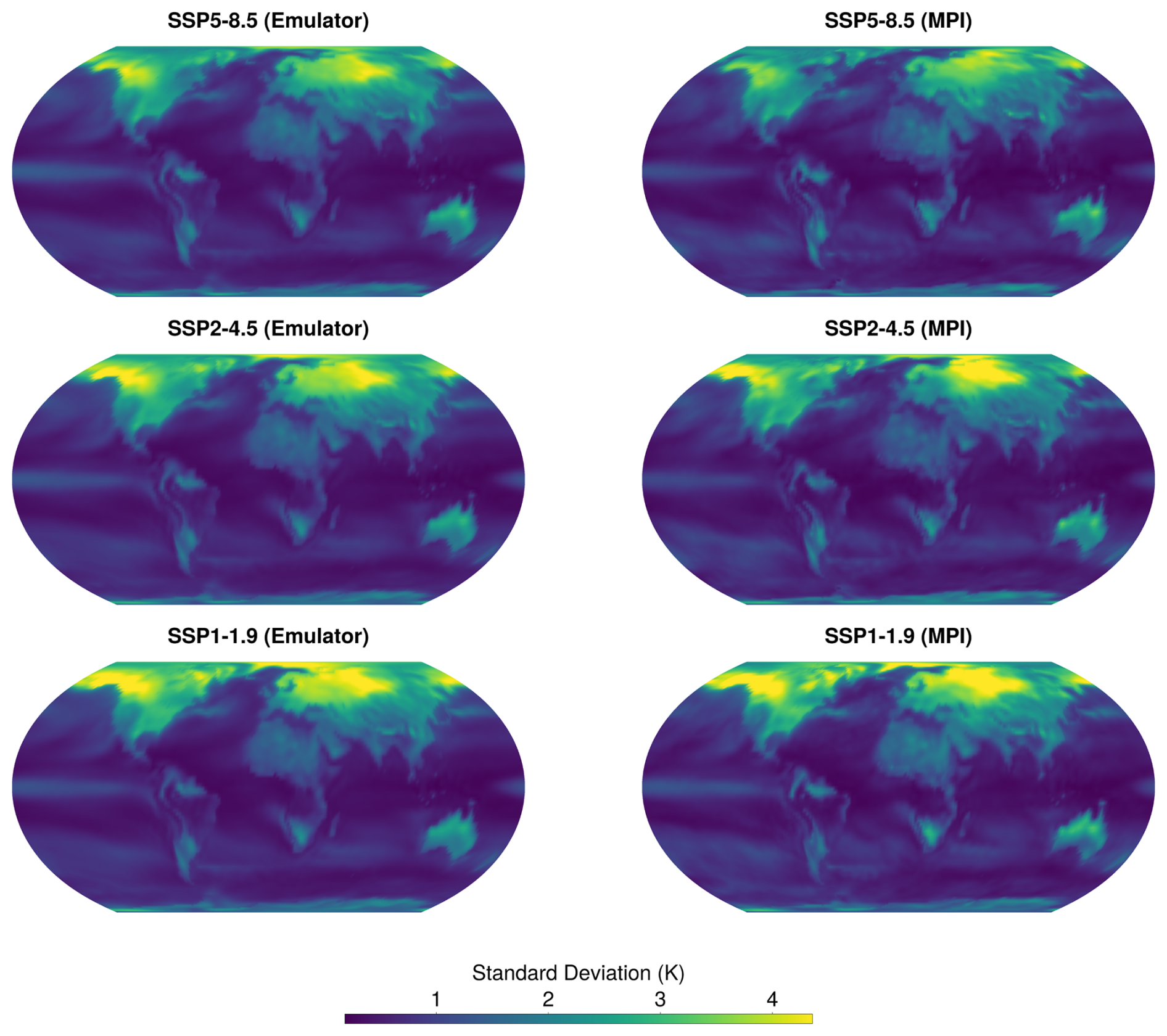
Figure D5 Emulator representation of January standard deviation of surface temperature in 2100. Emulator representation on the left, MPI model data on the right for comparison.