Combining different views on internal climate variability of temperature over Europe

Internal climate variability (ICV) represents the intrinsic fluctuations within the climate system. Understanding how ICV varies across regions, seasons, and climatic conditions is crucial for detecting externally forced climate change and assessing future climate risks. It can also provide a useful benchmark for assessing climate model performance and the emergence of anthropogenically forced climate change. This study aims to compare ICV estimates obtained using different methods and data types. We focus on seasonal mean near-surface air temperature over Europe, utilizing data from 15 CMIP6 models, a 100-member MPI-ESM large ensemble, and three observational datasets. The ICV estimates are based on pre-industrial control simulations (Pidata), the Hawkins and Sutton (2009) residual-based method (HS09), regression-based removal of external forcings, and a single-model large-ensemble framework. The magnitude of ICV estimates generally decreases from northeastern to southwestern Europe on both annual and seasonal timescales, except during JJA, when the highest estimates shift southward. The highest ICV estimates are observed in DJF and the lowest at the annual timescale. Among all the methods, Pidata generally yields the highest ICV estimates across all seasonal and annual timescales, except during JJA. Based on the HS09 method, the similarity between the model-based estimates and the observations is most pronounced during DJF and at the annual timescale. However, this similarity is weaker when the regression-based method is applied, with the model-based estimates generally exceeding the observation-based ones. The projected changes in ICV show a tendency for reduced (enhanced) values in DJF (JJA). Although a north-south contrast emerges in other seasons, with declining (increasing) ICV in northern (southern) Europe, the overall spatial pattern indicates a reduction in projected ICV estimates across large parts of Europe, except during JJA.

1 Introduction

Internal climate variability (ICV) is defined as a natural variability within the climate system that occurs without external forcing involvement (Deser et al., 2010, 2014; Thompson et al., 2015; Chen et al., 2021). Uncertainty associated with the ICV is one of the major sources of climate change projection uncertainties, due to the unpredictability of the evolving processes and interactions within the climate system itself (Deser et al., 2010; Deser, 2020; Schwarzwald and Lenssen, 2022; Blanusa et al., 2023; Lehner and Deser, 2025).

The climate system is known to be a nonlinear dynamical system (Dethloff et al., 2007). The interactions between its components involve energy, momentum, and mass transfers, as well as feedbacks across various spatial and temporal scales (Palmer, 1999; McWilliams, 2007; IPCC, 2021a). Nonlinearity and the resulting chaoticity in the system mean that just a small perturbation in the initial conditions can expand exponentially, leading to uncoupling of originally close climate system trajectories. For this reason, the climate system exhibits sensitive dependence on initial conditions, making its internal variability unpredictable beyond a certain time horizon (Lorenz, 1963; Ghil and Lucarini, 2020). This dependence, together with models' imperfections, limits the reliability of projections after the initial condition information has been lost, typically a few years (or even less than a year) for the climate projections (Lorenz, 1963, 1996) and as little as 10 d for weather prediction (Krishnamurthy, 2019). This eventually affects the climate projection outcome and contributes to the irreducibility of ICV uncertainty (Deser et al., 2010, 2014; Kay et al., 2015; Olonscheck and Notz, 2017; Jain et al., 2023). Moreover, the ICV is perceived through some modes of variability with intrinsic randomness (such as El Niño Southern Oscillation, Atlantic Multidecadal Variability, Pacific Decadal Variability, etc.), which arise from the system's dynamics (Collins et al., 2010; Deser et al., 2010; IPCC, 2021b). These might evolve unpredictably to some extent, and their future phase and amplitude are intrinsically uncertain (Ghil and Lucarini, 2020; Jain et al., 2023). This intrinsic unpredictability directly contributes to uncertainty in climate projections. Besides ICV, there are two other main sources of uncertainty in climate change projections, known as model uncertainty and scenario uncertainty. This division is helpful not only for scientific interpretation and improving climate models but also for science communication (Knutti and Sedláček, 2012; Abramowitz et al., 2019). Model uncertainty, also called climate response uncertainty, is attributed to structural differences between models and how they respond to external forcing. In principle, this uncertainty is reducible since the differences between models and between models and observations are artifacts of model imperfection (Abramowitz et al., 2019; Lehner et al., 2020; Merrifield et al., 2023). Scenario uncertainty or radiative forcing uncertainty arises from a lack of knowledge of future radiative forcing, which is primarily driven by unpredictable socio-economic factors (Hawkins and Sutton, 2009; Lehner et al., 2020). Unlike model uncertainty, scenario uncertainty is irreducible since the probability of future evolution of anthropogenic factors is currently unknown (Gosling et al., 2012; Lehner et al., 2020; Deser and Phillips, 2023).

Conceptually, ICV represents the intrinsic “noise” of the climate system. Therefore, the ICV estimate has been widely used as a “benchmark” for assessing the climate model outputs. Here, the term “benchmark” is not used in the sense of directly evaluating model skill in reproducing ICV. Rather, the ICV estimate is employed as a reference scale against which model performance and projected changes are assessed. Model biases smaller than the estimated ICV can be interpreted as being within the range of internal variability and thus indicate that the simulated values of the characteristics of interest cannot be reliably distinguished from the observations. In this sense, it is then possible to imply adequate simulation, or good accordance between simulated and observed values. Similarly, projected changes that do not exceed the ICV may be considered indistinguishable from internal variability, and hence not statistically robust. While ICV represents internal fluctuations, external forcing can modulate both the mean climate and the characteristics of variability itself. Understanding how ICV varies across regions, seasons, and climatic conditions is therefore crucial for detecting externally forced climate change and for assessing future climate risks. However, ICV cannot be directly observed and must be inferred from observations or model simulations. Different methods and data sources can yield substantially different estimates of ICV magnitude.

The evidence for human influence on recent climate change reported from IPCC AR2 to AR5 has become stronger over the last few decades (IPCC, 2021c). This human influence includes increasing greenhouse gas concentrations, changes in land use, and emissions of human-made aerosols (e.g., sulfates, black carbon). In sum, these effects have led to positive radiative forcing, resulting in increased observed warming (IPCC, 2021c). The anthropogenic influence resulting in forced climate change not only modulates the mean climate but also the characteristics of ICV itself and the overall climatic variability and extremes (Deser et al., 2010; LaJoie and DelSole, 2016; Rodgers et al., 2021; Deser and Phillips, 2023). One among other examples, a recent study by Beobide-Arsuaga et al. (2025) found that forced changes in internal variability will intensify summer heatwaves over central and northern Europe, while they are projected to weaken southern European summer heatwaves. Many studies illustrate how external forcing might change internal variability characteristics (Deser et al., 2010; LaJoie and DelSole, 2016; Rodgers et al., 2021; Deser and Phillips, 2023). Thus, to more accurately assess climate change on various temporal and spatial scales, it is essential to evaluate the ICV and its interaction with both natural and anthropogenic influences, and to estimate how climate change influences the ICV itself.

One of the early methods to estimate the ICV as a benchmark for climate model outputs was applied in Giorgi and Mearns (2002). They estimated the ICV as the range between the minimum and maximum of running 30-year averages of detrended seasonal mean temperature or precipitation, using long observed time series. Later, Hawkins and Sutton (2009) assessed ICV by using historical and scenario simulations from global climate models. They fit a fourth-order polynomial to the simulated time series and assessed the ICV magnitude from the fit residuals. This method has been applied for partitioning model uncertainty in many other studies using climate model datasets (Hawkins and Sutton, 2011; Yip et al., 2011; Lehner et al., 2020; Snyder et al., 2024; Evin et al., 2024). One of the most widely used approaches to ICV assessment involves pre-industrial control simulations (Olonscheck and Notz, 2017; Menary et al., 2018; Rehfeld et al., 2020; Van Achter et al., 2020; Sippel et al., 2021; Mann et al., 2022; Zappa et al., 2021). These provide long time series spanning from hundreds to thousands of years and are run under fixed conditions at pre-industrial levels (typically year 1850; Eyring et al., 2016). Thus, there is no influence of changes in external forcings, and any variability in the simulation comes solely from internal processes of the climate system. Further, Single-Model Initial-condition Large Ensembles (SMILEs) simulations are considered robust tools for assessing ICV since they are created using a single climate model run under the same external forcing but with slightly different initial conditions, which is designed to isolate ICV from other uncertainties (Lehner et al., 2020; Deser, 2020; Maher et al., 2021). Depending on the computational capacity of each modeling center, a SMILE typically consists of 30 to 100 members. Many studies have successfully used one or more SMILEs to examine ICV behavior, including Kay et al. (2015), Martel et al. (2018), Maher et al. (2020), Lehner et al. (2020), and Shen et al. (2024), among others. Another approach to quantifying ICV magnitude is to look into the observed climate variability and to attempt its attribution to external and internal forcings (e.g., Foster and Rahmstorf, 2011; Mikšovský et al., 2016). If the influence of external forcings can be estimated and the forced signal can be subtracted from the observed time series, the resulting residuals represent the estimate of ICV.

Despite the wide range of approaches, a systematic comparison of ICV estimates across methods and datasets, including observational constraints, remains lacking – particularly at the regional scale over Europe. Given that each of the above-mentioned methods and datasets plays a valuable role in assessing ICV, this study combines, for the first time, several approaches and datasets to compare and assess ICV magnitude from diverse perspectives. We focus on the annual and seasonal means of near-surface air temperature. Specifically, the study aims to quantify historical and future ICV levels across Europe, to evaluate the magnitude of uncertainty in ICV estimation using different approaches, and to characterize the spatial distribution of ICV over Europe and its evolution under future conditions.

2 Study area

The study area encompasses the European region, divided into four subdomains, as shown in Fig. 1. Three of the four subregions were defined based on the updated IPCC WGI reference regions (Iturbide et al., 2020) and are noted as NEU (Northern Europe), WCE (Western and Central Europe), and MED (Mediterranean). The last subregion, denoted CEU (Central Europe) and bordered by the dashed rectangle in Fig. 1, is of interest for climate change scenarios in the Czech Republic and surrounding regions, especially for convection-permitting regional climate model simulations that focus on this region. The ICV estimates developed in the current study will be further used as a benchmark for assessing model performance and future climate change projections over this area.

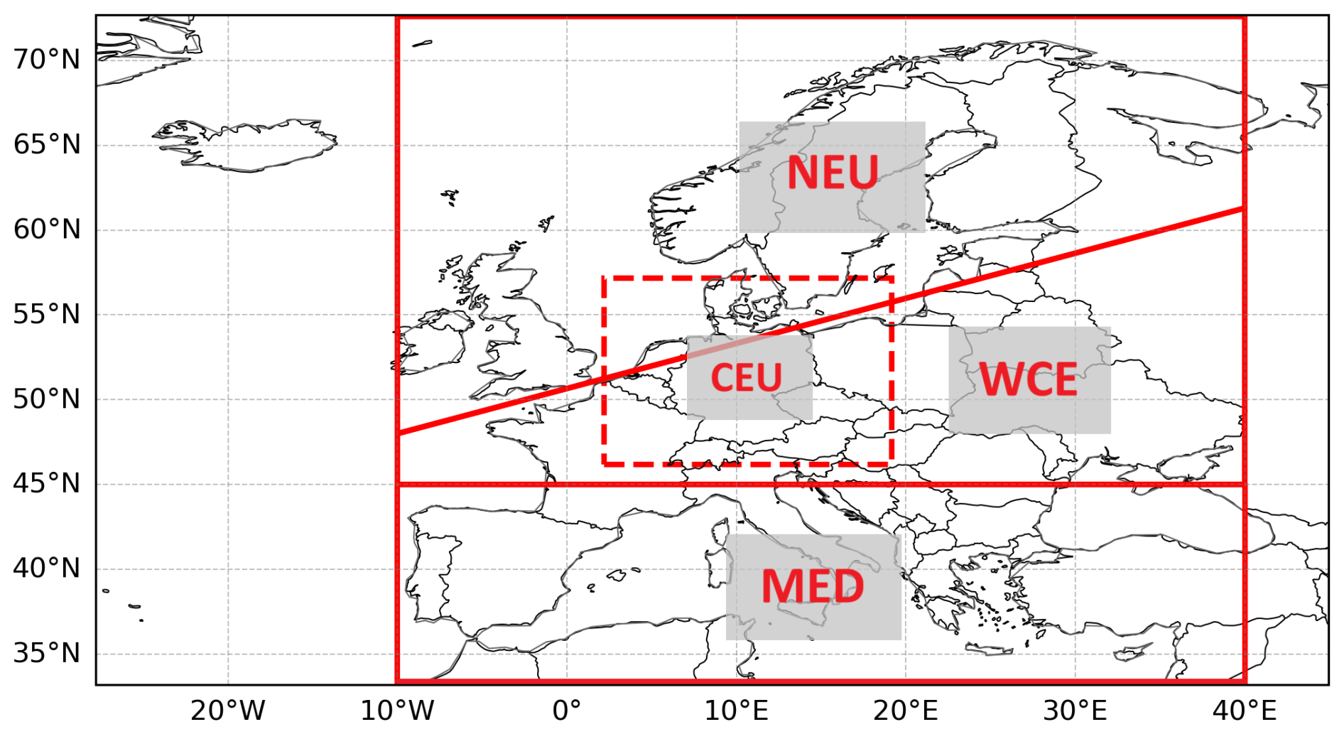
Figure 1 Subregions used in this study. The subregions within the red solid contours, from north to south, are the NEU, WCE, and MED domains, and the dashed red contour pertains to the CEU domain.

3 Methods and data

3.1 Data

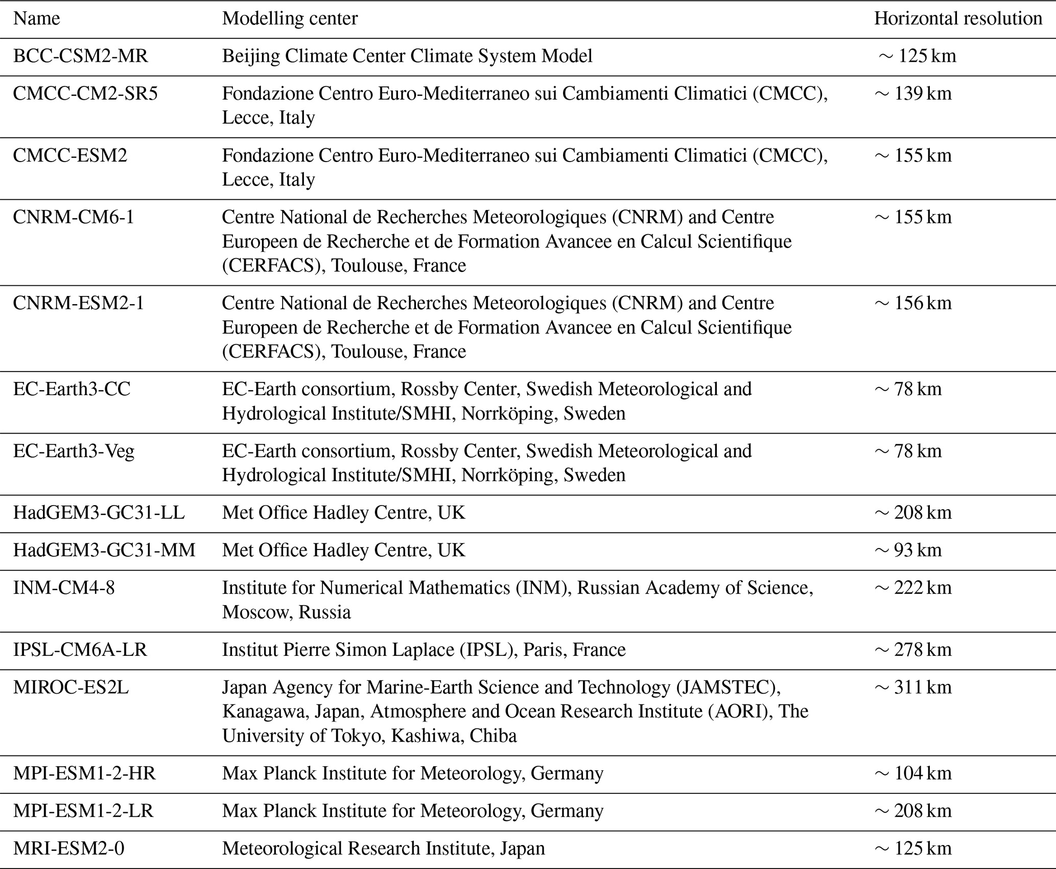
We use 15 models from CMIP6 global climate models (GCMs, Eyring et al., 2016), listed in Table 1. These 15 models were selected because they provide 500 years (with years designated as from 1850 to 2349) of continuous pre-industrial control simulations (hereafter referred to as Pidata) suitable for our analysis, ensuring consistent inputs. The same set of 15 CMIP6 models was subsequently analyzed for the historical (1971–2000) and future (2070–2099) periods. The future period was obtained from simulations following the SSP5-8.5 scenario. We selected SSP5-8.5 because it represents the upper range of available CMIP6 forcing pathways and is associated with the strongest anthropogenic influence on the climate system. Consequently, potential externally forced changes in ICV are expected to be more pronounced and therefore easier to detect than under lower-emission scenarios. The resulting subset represents 7 of the 14 CMIP6 model families (Brunner et al., 2020), with equilibrium climate sensitivities ranging from 1.8 to 5.6 °C (Meehl et al., 2020).

Table 1 Global climate models used for Pidata and CMIP6.

In addition, we use one single-model initial-condition large ensemble (SMILE) in this study, namely the MPI-ESM model. This SMILE comprises 100 members (Maher et al., 2019), which, to the best of our knowledge, is the largest ensemble currently available. The simulations were performed at a horizontal resolution of 1.875° × 1.875° (longitude × latitude) and include scenario runs under RCP8.5 (Maher et al., 2019). Although RCP8.5 differs slightly from SSP5-8.5 used for CMIP6, for the purpose of this study, we neglect the differences in their radiative forcing trajectories.

Table 2 Observational datasets.

Finally, we employ three observationally based temperature datasets (Table 2), including one reanalysis product and two gridded observational datasets. These datasets differ in spatial resolution and methodological approach, and their comparison provides an estimate of observational uncertainty.

For comparison purposes, we regridded all the results into a common grid of 1° × 1° (longitude × latitude) using bilinear interpolation in Climate Data Operators (CDO) (Schulzweida, 2022). The 1° resolution was chosen because many models have resolutions around 1°, making it a middle ground. Moreover, comparisons between the original and regridded grids show almost no difference (Fig. S1 in the Supplement). We first computed the ICV estimates for the datasets at their original grid based on the methods described in the methodology section (Sect. 3.2) and then regridded all of them into the common grid. This is done to retain as much of the information from their original grids as possible. Then, we calculated spatial mean of each region. The spatial aggregation was done using “cdo fldmean,” and it accounts for area weighting (Schulzweida, 2022). It should be noted that the land-sea mask dataset has a relatively coarse spatial resolution (1° × 1°). As a result, the spatial extent of the masked regions may appear inconsistent with the actual coastlines, represented by the thin country-border lines in the figures (Figs. 2–4).

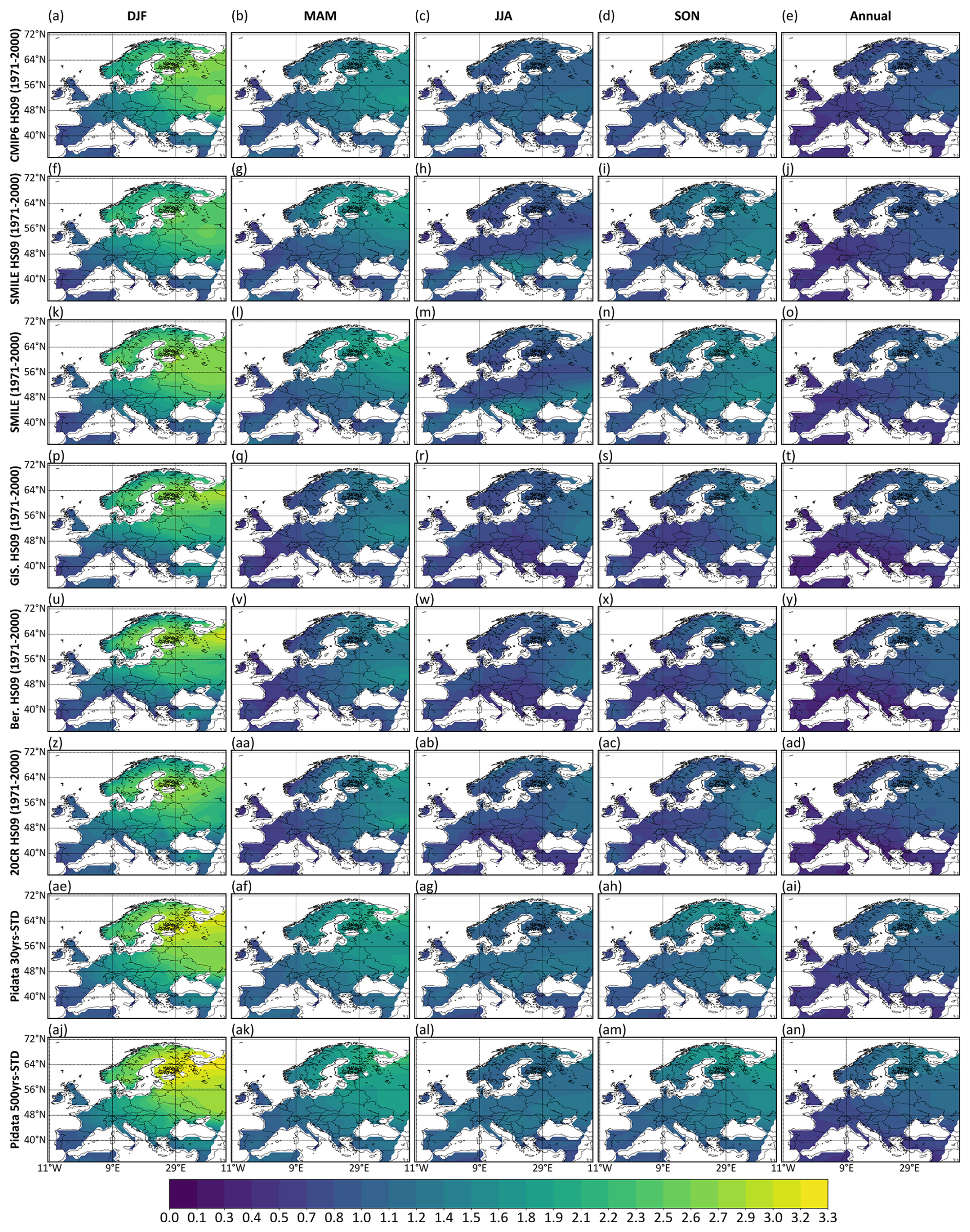
Figure 2 Annual and seasonal means of ICV estimates of temperature. The estimates based on the HS09 method during the period 1971–2000 are applied for the case of CMIP6 (first row), SMILE MPI-ESM (second row), GISTEMP (fourth row), Berkeley (fifth row), and 20CR (sixth row). The third row provides the estimates based on the SMILE TYP method for the 1971–2000 period. The last two rows are the estimates based on the Pidata SD method. “Pidata 30yrs-STD” refers to the ENSMEAN based on the Pidata 30yrs-STD method. “Pidata 500yrs-STD” refers to the ENSMEAN based on Pidata 500yrs-STD method. CMIP6 and SMILE represent the ENSMEANs of CMIP6 and SMILE MPI-ESM, respectively. Unit: [°C].

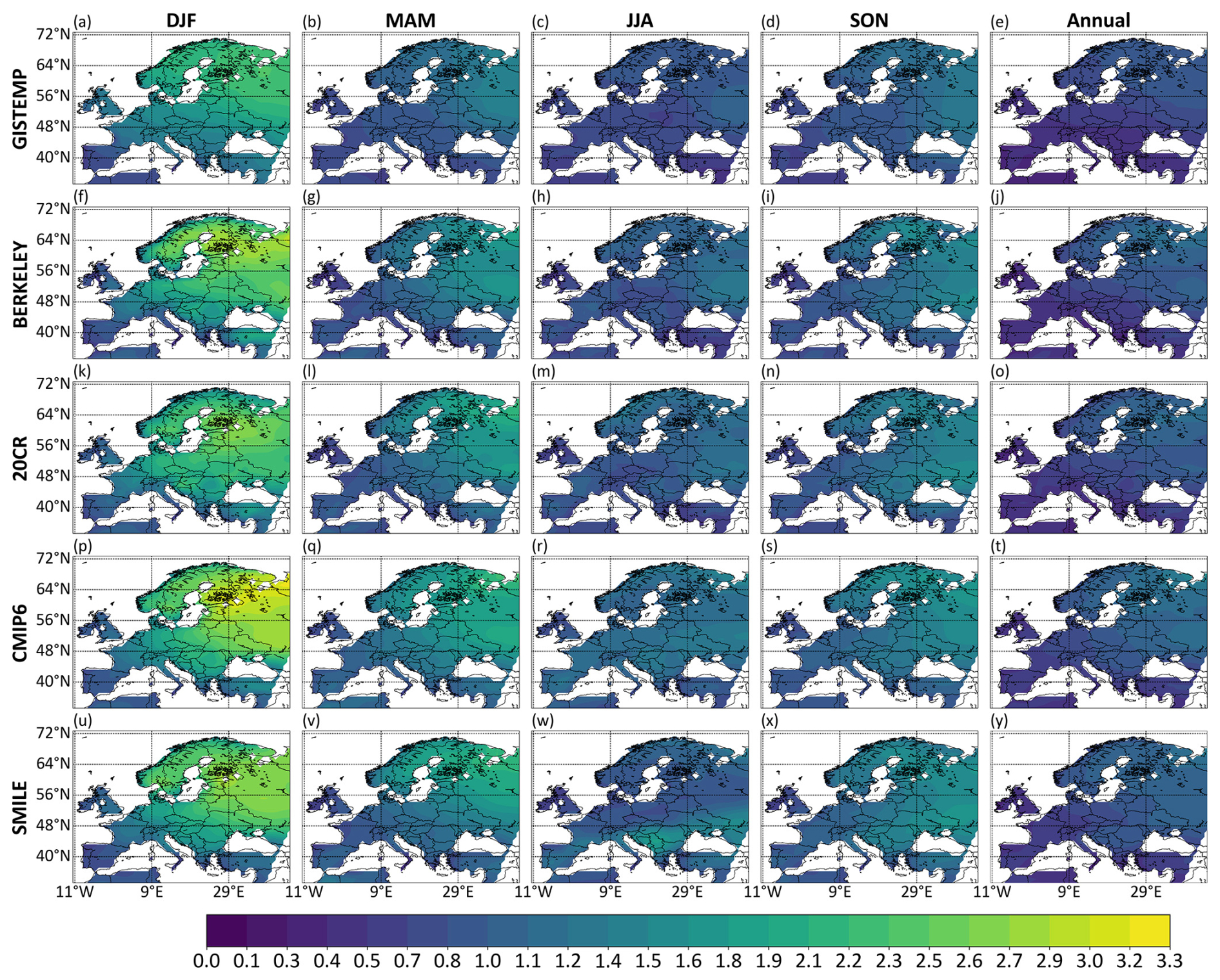
Figure 3 Annual and seasonal means of ICV estimates of temperature based on the REG method applied to the three observational datasets (GISTEMP, Berkeley, and 20CR), CMIP6 and MPI-ESM SMILE during the period 1901–2010. Unit: [°C].

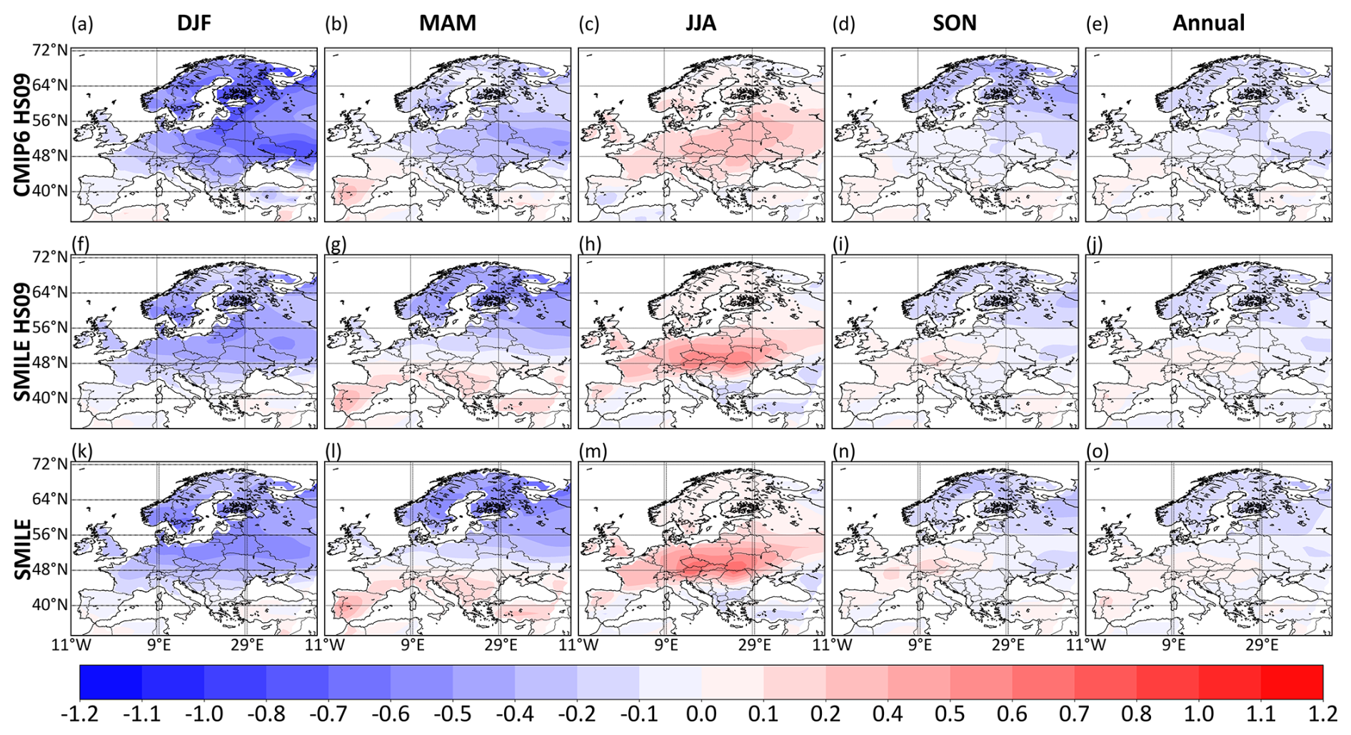
Figure 4 Annual and seasonal differences between the future and historical ICV estimates using the HS09 method for CMIP6 (first row) and SMILE MPI-ESM (second row) and using the SMILE TYP method for the third row. Unit: [°C].

3.2 Methods

3.2.1 Calculation of ICV from pre-industrial control simulations

For the case of Pidata, the analysis of ICV was done through the computation of standard deviation (SD) (Olonscheck and Notz, 2017). The simulations are not influenced by any changes in external forcings, so all temporal variability in modelled time series is attributed to ICV. First, the simulated temperature time series were linearly detrended, so that the effect of an artificial drift would not contaminate the estimate of ICV (Gupta et al., 2013). We computed seasonal and annual timeseries and detrended each of the timeseries before the SD calculation. We have also investigated temporal trends and detected no notable temporal trends in any of the time series. We then calculated SD of each of these timeseries for each model. In this study, we applied SD for two different types of analyses. We calculated SD for non-overlapping 30-years period timeseries within the period 1850–2349. Therefore, for each of the models, we have 16 SD values on each of the seasonal and annual time scales. This method is hereafter noted as “Pidata 30yrs-STD”. For each model, we calculated the mean of these 16 SD values (denoted further as “Mean 30yrs-STD”). The ENSMEAN then refers to the mean over the 15 models. We also computed SD for 500-years period timeseries (for the period 1850–2349), which yields one SD value for each of the models on each of the seasonal and annual time scales. This method is hereafter denoted as “Pidata 500yrs-STD”. The ENSMEAN from Pidata 500yrs-STD refers to the mean over the 15 models.

3.2.2 Hawkins and Sutton (2009) method

The method of Hawkins and Sutton (2009) (further noted as HS09) was employed to assess the magnitudes of ICV under the existence of external forcings. We applied the HS09 method to each of the CMIP6 models and each of the MPI-ESM SMILE members during both the historical (1971–2000) and the future scenario (2070–2099) periods and to the three observational datasets during the historical period. Additionally, in the Supplement, we applied the method during the whole period (1971–2100) to the CMIP6 simulations. The methodology is described as follows. First, seasonal and annual anomalies were calculated during the study periods. These anomaly time series were then smoothed by fitting a fourth-order polynomial using ordinary least-squares regression. Subsequently, the smoothed anomalies were subtracted from the original anomalies to obtain the residual component, denoted as Epsilon. Finally, the ICV was quantified as the standard deviation of the Epsilon. Throughout the study, for the historical and scenario CMIP6 simulations, ENSMEAN refers to the mean of the 15 selected models, while for the case of SMILE MPI-ESM simulations, ENSMEAN refers to the mean of the 100 members.

3.2.3 Calculation of ICV using regression analysis

To remove components attributable to external forcings, we also applied a regression model, leaving only ICV-related variability in the regression residuals. The temperature time series at individual grid points for the period 1901–2010 were processed using multiple linear regression, with predictors pertaining to greenhouse gas concentration, volcanic aerosol optical depth, and solar activity, as described in Mikšovský et al. (2016). The residuals were then aggregated to seasonal and annual means, and the ICV was estimated as the standard deviation of the aggregated time series. This approach was applied to observational data and historical CMIP6 and SMILE MPI-ESM simulations. The linear regression method is further referred to as REG method.

3.3 Calculation of ICV based on SMILE typical method

In addition to the HS09 and regression-based approaches, we also estimated ICV based on SMILE MPI-ESM simulations using the method commonly adopted in many previous studies (e.g., Martel et al., 2018; Maher et al., 2020; Lehner et al., 2020), hereafter referred to as the SMILE TYP method. Seasonal and annual anomalies were first computed relative to the long-term mean during both the historical (1971–2000) and scenario (2070–2099) periods for each SMILE MPI-ESM member. Subsequently, the ensemble mean anomaly, representing the forced signal, was calculated across all 100 ensemble members and removed from each member's anomaly. This procedure isolates the internally generated variability by eliminating the influence of the forced distribution shift. The ICV estimate was then quantified as the standard deviation of these residual anomalies across the 100 ensemble members, with each member has 30 years timeseries of the residual anomaly.

4 Results

4.1 Spatial distribution of ICV estimates

In general, the spatial distributions of the ICV estimates for both annual and seasonal timescales show a similar pattern between all methods and time periods (Figs. 2 and 3). The highest values are in most cases found over the north-eastern part of the study domain, except during the summer season, while the lowest values are depicted over the southern part, starting from 0.2 °C. Looking into details, the annual analysis exhibits weaker ICV estimates up to 1.7 °C. The DJF season shows the highest values, reaching up to 3.3 °C. All the methods indicate that the largest values are found over north-eastern Europe, where Pidata, Berkeley HS09-based, and CMIP6 REG methods display ICV estimates exceeding 3.0 °C. In MAM, the ICV values are slightly lower than in DJF, with values up to 2.5 °C. In the case of JJA, the highest ICV estimate is about 1.7 °C, but the higher estimates shift southward and cover the latitudes between 40 and 56° N. The SON pattern is similar to DJF and MAM but with values up to 1.9 °C. Overall, ICV estimates across the European region decrease from north-east to south-west on both annual and seasonal timescales, except during JJA, when the highest ICV magnitudes move southward. The smallest ICV estimates are depicted on the annual scale over the MED region, while the largest estimates are found in DJF over northwestern Europe.

Pidata SD methods (Fig. 2) generally produce the largest ICV estimates across the different approaches and timescales over northwestern Europe, except during JJA. Within the Pidata framework, the 500yrs-STD estimates systematically exceed those derived from the 30yrs-STD, demonstrating a clear dependence of ICV magnitude on the length of the underlying time series. A similar behaviour is found for SMILE (Fig. 2), where the SMILE TYP method consistently yields higher ICV estimates than the HS09 formulation. Taken together, these results indicate that longer records tend to amplify the estimated ICV, likely reflecting an improved sampling of low-frequency variability. In addition, the HS09-based method (Fig. 2) shows that the observational estimates display a spatial pattern similar to that of model-based results during DJF, characterized by decreasing ICV estimates from northeast to southwest, whereas the pattern differs slightly in the other seasons. The range of ICV values derived from CMIP6 HS09 and SMILE HS09 generally falls within the ranges obtained from the observational HS09-based estimates across most seasons. This consistency suggests that the HS09 methodology provides a robust basis for comparing internally generated variability between observations and model ensembles. For the REG method (Fig. 3), all datasets exhibit broadly similar spatial patterns in DJF, MAM, and for annual timescales. However, the magnitude of the estimated ICV slightly differs among datasets, with model-based estimates generally exceeding those derived from observations. Among the model datasets, the CMIP6 ENSMEAN consistently produces the largest ICV estimates. This suggests that climate models may simulate stronger ICV than is inferred from observations, although the large-scale spatial characteristics remain similar among datasets in DJF, MAM, and for annual timescales.

Figure 4 illustrates projected changes in the ICV estimates, calculated as the difference between future and historical ICV estimates. The analysis was conducted using three approaches: CMIP6 HS09, SMILE HS09, and SMILE TYP methods, at both seasonal and annual timescales. During DJF, all three methods consistently indicate a reduction in ICV across most of the study area, with changes ranging from approximately −1.0 to −0.1 °C. Positive changes are confined to the MED region, where values reach up to 0.2 °C. Nevertheless, the majority of the domain exhibits negative changes exceeding −0.5 °C over most parts of the study area, suggesting considerably weaker future ICV compared with the historical period. In contrast, JJA is characterized by predominantly positive changes across the study area. Future ICV estimates exceed historical values over most regions, with increases reaching up to 0.7 °C. Negative changes are restricted mainly to the MED region, where values decrease to approximately −0.2 °C. These results indicate an overall enhancement of ICV during summer under future climate conditions. The spatial pattern in MAM resembles that of DJF, although positive changes are more widespread and stronger, reaching up to 0.4 °C over the MED region and extending northward. Concurrently, areas exhibiting negative changes shrink toward higher latitudes, reaching −0.9 °C. Changes during SON are generally weaker than in the other seasons. Positive values, up to 0.2 °C, occur over the MED, the CEU, and parts of the eastern study area, whereas negative values reaching approximately −0.5 °C are found across northern regions, particularly over large parts of NEU. The annual results display a spatial pattern similar to that observed in SON but with weaker amplitudes, ranging from approximately −0.4 to 0.1 °C. Overall, the projection of ICV estimates indicates a substantial decrease in ICV during winter (DJF) across most regions, whereas summer (JJA) is characterized by widespread increases relative to the historical period. During MAM, SON, and on the annual timescale, a clear north-south contrast emerges, with lower future ICV estimates over northern regions and higher future ICV estimates over southern regions compared with historical conditions.

Additionally, the annual ICV estimates for each of the 15 individual CMIP6 models are shown in the Supplement to provide inter-model comparison (Figs. S2–S5). We applied the 500yrs-STD method to Pidata and the HS09 method to the historical, scenario, and whole periods. Pidata display the highest ICV estimates for each individual model (Fig. S2), whereas the scenario simulations show the lowest values for each model (Fig. S4). BCC-CSM2-MR model simulates the highest ICV magnitude among all other models in all the approaches, while EC-Earth3-CC and EC-Earth3-Veg models show a remarkably high ICV in Pidata (Fig. S2), especially over the extreme north of the study area. Unlike in Pidata, in which the higher values decrease from the north-east to the south for all models (Fig. S2), some models in the historical and scenario simulations display different patterns. For instance, CMCC-EMS2, CNRM-ESM2-1, EC-Earth-Veg, and HadGEM3-GC-MM show that the higher ICV estimates are located over the central part of the study domain (Figs. S3–S5). There are also some models that display different patterns depending on each period. This is the case for HadGEM3-GC-LL, INM-CM4-8, and MRI-ESM2, in which higher ICV estimates are observed across different locations. Overall, the Pidata 500-year SD for individual models yields the highest ICV estimates, followed by CMIP6 HS09 calculated over the full 130 years period (1971–2100). Applying CMIP6 HS09 to a shorter 30 years period results in lower ICV values, both for the historical (1971–2000) and future scenario (2070–2099) intervals. This hierarchy reinforces the earlier finding that ICV estimates increase with the length of the time series, underscoring the importance of long records for capturing low-frequency variability. In addition, the annual CMIP6 HS09 estimates for most of the models during the historical period are consistently higher than those of the scenario period. This difference may indicate a modulation of ICV under changing external forcing, although part of the contrast could also arise from sampling uncertainty (the choice of the specific time periods).

4.2 Regional mean analysis of ICV estimates

Figures 5–9 represent the intercomparison of ICV estimates averaged over the four regions based on the HS09 method applied to 30 years timeseries for the case of CMIP6 and SMILE, and the SD method applied to 30 and 500 years timeseries for the case of Pidata. Overall, DJF (Fig. 6) exhibits the highest ICV estimates, reaching values above 2.3 °C (as indicated by the PiData 500yrs-STD ENSMEAN over NEU). In contrast, annual mean estimates (Fig. 5) are the lowest, with a value of approximately 0.4 °C as displayed by the observational estimates over MED. Intermediate values are observed in MAM (Fig. 7), SON (Fig. 8), and JJA (Fig. 9). Regionally, the MED (NEU) consistently shows the smallest (highest) estimates compared to the other regions (Figs. 5–9).

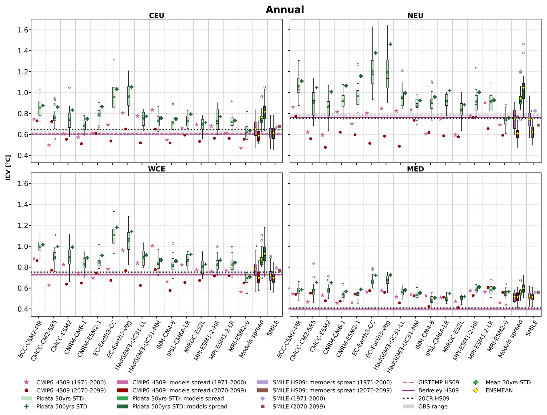
Figure 5 Annual ICV estimates based on the HS09 method applied to CMIP6, SMILE MPI-ESM (noted as SMILE in the figure), and the observational data, while the SD method is applied in the case of Pidata (represented with different green colors). “Pidata 30yrs-STD” refers to the spread of 16 SD values, each of which was obtained by the application of the SD method for 30 years timeseries. “Pidata 30yrs-STD: models spread” refers to the spread of the 15 CMIP models, in which each model is represented by the mean of the 16 SD values. “Pidata 500yrs-STD” is a single value from the application of SD for 500 years timeseries. “Pidata 500yrs-STD: models spread” refers to the spread of the 15 models based on “Pidata 500yrs-STD”. “OBS range” represents the difference between the maximum and minimum values among the three observational datasets. “Mean 30yrs-STD” refers to the mean of the “Pidata 30yrs-STD”. “ENSMEAN” refers to the multi-model mean or multi-member mean as described in the methodology section.

Figure 6 Same as Fig. 5 but for DJF season.

Figure 7 Same as Fig. 5 but for MAM season.

Figure 8 Same as Fig. 5 but for JJA season.

Figure 9 Same as Fig. 5 but for SON season.

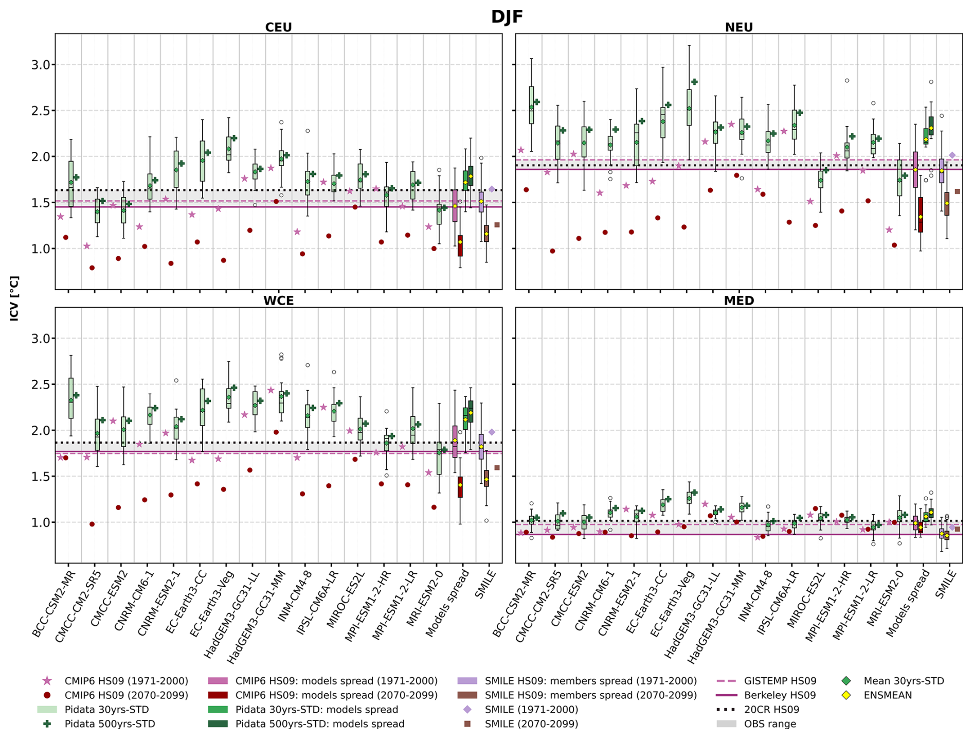
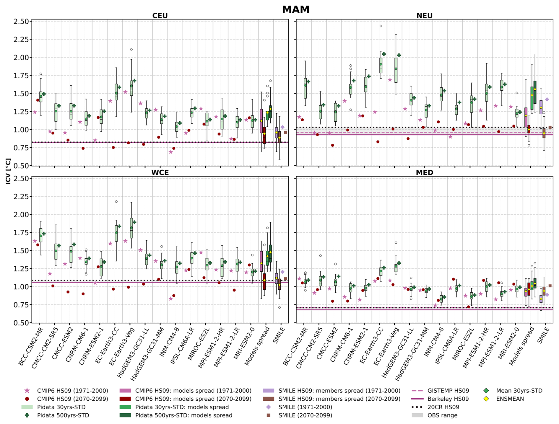
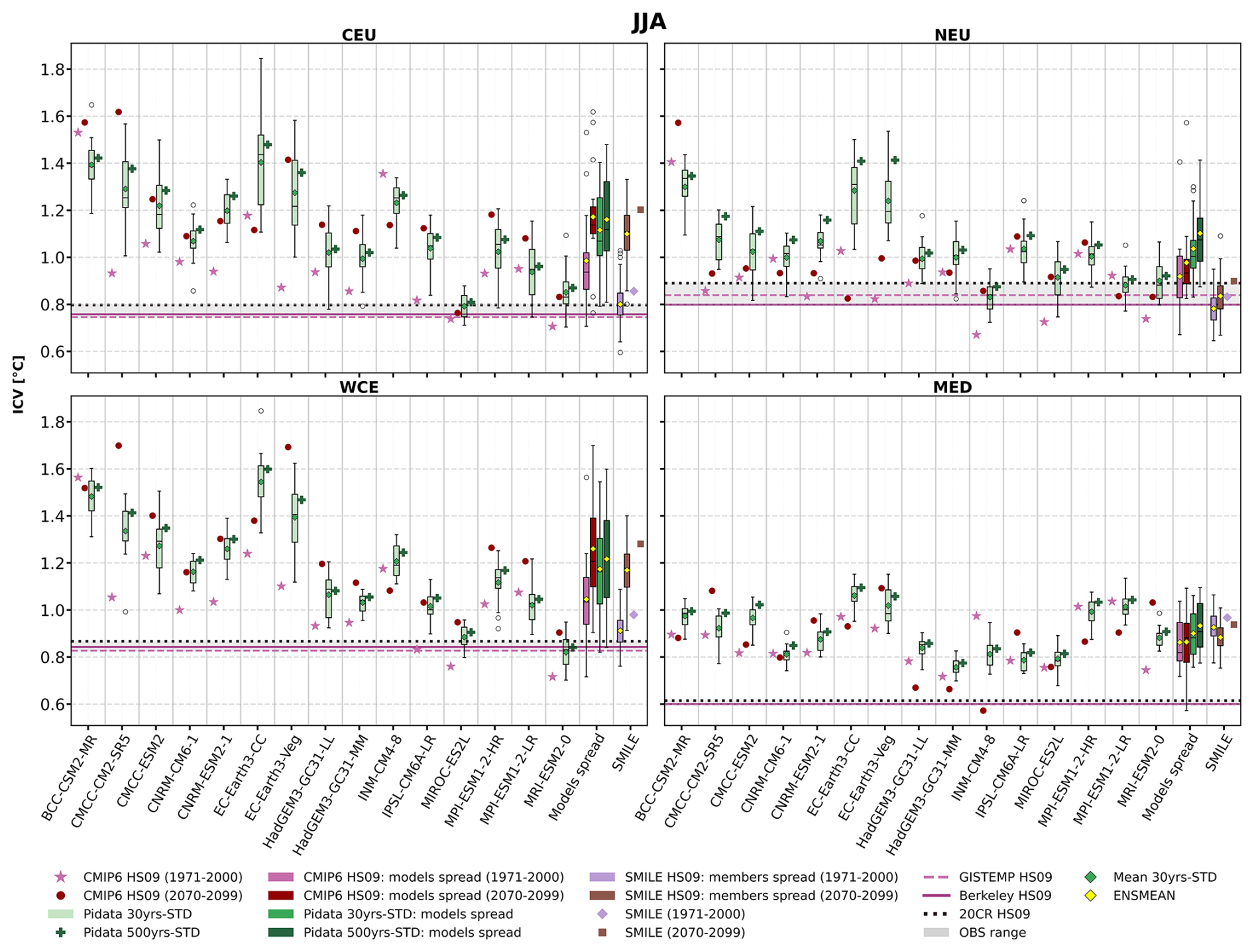
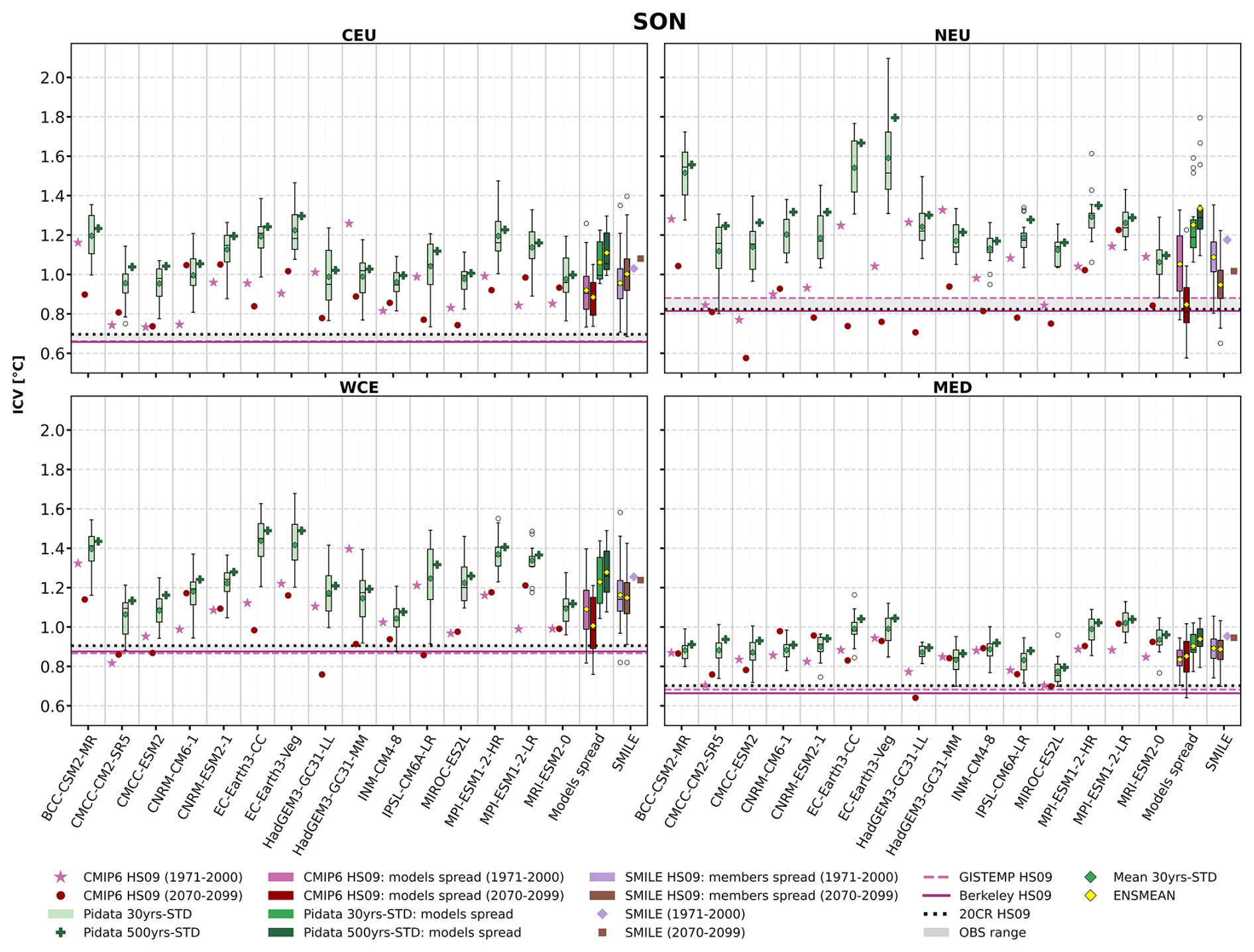
Considering inter-method comparison, ICV estimates derived from the Pidata are generally the highest, except during JJA over CEU and WCE. This is evident by looking at the ENSMEAN values, where Pidata ENSMEAN values exceed the ICV estimates from all the other methods (Figs. 5–9). Substantial inter-model variation is observed, with the EC-Earth model based on the Pidata SD method producing the highest ICV estimates among all other models (Figs. 5–9). In addition, the ENSMEAN of 500yrs-STD approach systematically yields larger ICV estimates than the ENSMEAN derived from the 30yrs-STD method. When comparing different methodological approaches applied to SMILE (Figs. 5–9), the HS09 method consistently produces lower ICV estimates than the SMILE TYP method across all seasons and regions. These results confirm what was found earlier during the spatial analysis, i.e., longer records tend to amplify the estimated ICV, likely reflecting an improved sampling of low-frequency variability.

A direct comparison between SMILE and CMIP6 simulations highlights both consistencies and discrepancies (Figs. 5–9). During the historical period, HS09-based ICV estimates derived from both ENSMEANs of CMIP6 and SMILE simulations exhibit similar values, with differences of no more than 0.04 °C over the CEU and WCE regions at the annual timescale (Fig. 5). A similar level of agreement is observed during DJF (Fig. 6). In MAM (Fig. 7), however, larger discrepancies emerge, with CMIP6 ENSMEAN values generally exceeding those from SMILE in all regions except over the NEU. Similarly, during JJA (Fig. 8), CMIP6 ENSMEAN estimates are consistently higher than SMILE ENSMEAN values across all regions, except in the MED. In SON (Fig. 9), differences between the two model-based results are comparatively small, although SMILE estimates become slightly higher than CMIP6 over all regions. For the future period, CMIP6 and SMILE HS09-based ICV estimates display similar values at the annual timescale (Fig. 5) across all regions. During DJF (Fig. 6), however, SMILE ENSMEAN estimates tend to be slightly larger than those obtained from CMIP6, with an exception over the MED. In MAM (Fig. 7), in contrast to the historical period, the future period displays generally smaller differences between the two model-based results, with CMIP6 ENSMEAN values slightly exceeding those from SMILE ENSMEAN across all regions. During JJA (Fig. 8), CMIP6 continues to produce higher ENSMEAN estimates than SMILE in most regions, except over MED. Conversely, in SON (Fig. 9), SMILE ENSMEANs exhibit higher estimates than those of CMIP6 ENSMEANs across all regions. Overall, the historical ICV estimates derived from CMIP6 ENSMEAN and SMILE ENSMEAN display similar values during DJF and at the annual timescale, with only minor differences that do not exceed 0.04 °C across the regions. Larger discrepancies emerge during MAM and JJA, when CMIP6 ENSMEAN generally produces higher ICV estimates than SMILE ENSMEAN across most regions. In SON, differences between the two ensembles are smaller, although SMILE ENSMEAN tends to yield slightly higher estimates than CMIP6 ENSMEAN. A similar overall pattern is found for the future period. CMIP6 and SMILE ENSMEAN exhibit similar estimates at the annual timescale, whereas SMILE ENSMEAN generally exceeds CMIP6 ENSMEAN during DJF and SON in most regions. In contrast, CMIP6 ENSMEAN produces slightly larger ICV estimates during MAM and JJA. Furthermore, the inter-model spread of CMIP6 is generally larger than the spread among SMILE members. This finding suggests that uncertainties associated with structural differences among climate models are greater than those arising from different realizations of a single model.

A comparison of historical and projected ICV estimates derived from the CMIP6 HS09, SMILE HS09, and SMILE TYP methods (Figs. 5–9) reveals a clear seasonal dependence in the projected changes. At the annual and DJF timescales, historical ICV estimates are generally larger than their future counterparts across all regions. A similar pattern is observed during MAM, with the exception of the MED region. In contrast, during JJA, future ICV estimates exceed historical values across nearly all regions, except over MED. During SON, higher historical than future ICV estimates re-emerge over most regions, although the SMILE simulations indicate an opposite behaviour over CEU. In summary, the projected changes in ICV are strongly season- and region-dependent, with a tendency towards reduced ICV in winter and annual means, but enhanced ICV in summer.

The results of HS09 applied to SMILE, CMIP6, and observational datasets demonstrate varying levels of consistency depending on the season. On the annual scale (Fig. 5), historical ICV estimates from CMIP6 and SMILE display values within the range of observational estimates across most regions, as indicated by their ENSMEAN values, except over the MED, where model-based estimates are higher. A similar level of agreement is found in DJF (Fig. 6) across all regions. In contrast, during MAM (Fig. 7), historical CMIP6 ENSMEAN and SMILE ENSMEAN values exceed observational estimates in all regions. During JJA (Fig. 8), CMIP6 and SMILE estimates remain higher than observations across most regions, apart from NEU. A similar pattern is observed in SON (Fig. 9), where historical CMIP6 and SMILE estimates generally exceed observational values in all regions. Overall, the difference among the observational datasets is smaller than that among the model-based datasets across all regions and timescales (Figs. 5–9). In addition, the inter-model spread of CMIP6 generally exceeds the spread among SMILE members in most cases. These findings suggest that uncertainties associated with observational datasets are relatively minor compared with those arising from climate model structural differences. While the uncertainties stemming from structural variations across climate models are larger than those resulting from multiple realizations of a single model.

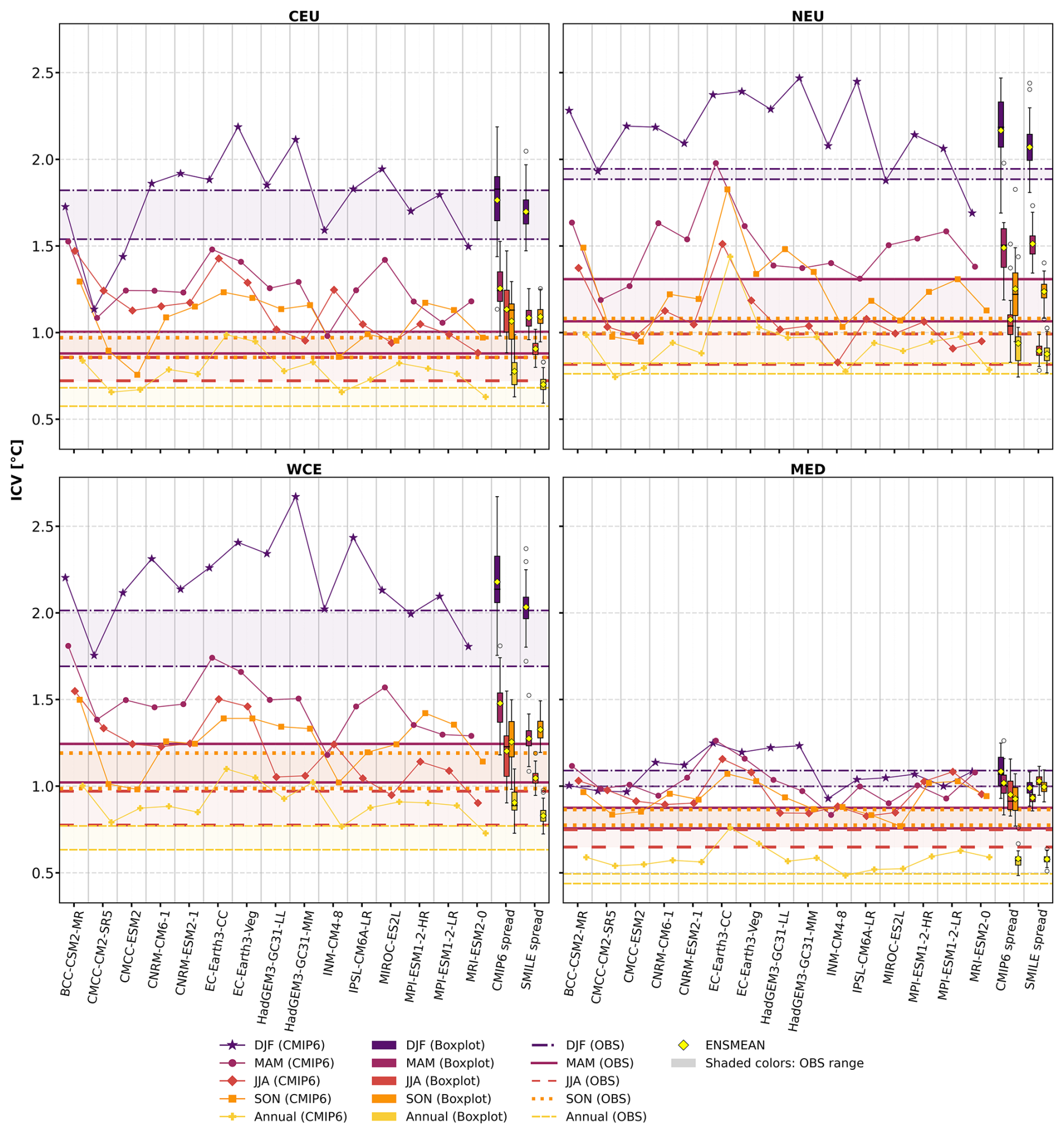
Figure 10 Seasonal and annual ICV estimates based on the REG method during the period 1901–2010 applied to each of the CMIP6 models, the three observational datasets, and SMILE MPI-ESM members. “CMIP6 spread” gives the spread of the 15 CMIP6 models. “SMILE spread” gives the spread of the 100 members of the SMILE MPI-ESM. The horizontal lines pertain to the observational data, in which the shaded colors represent the difference between the maximum and minimum values among the three observational datasets. OBS refers to the observational data.

Figure 10 represents ICV estimates averaged over the four regions using the REG-based method applied to CMIP6, SMILE, and the three observational datasets for the period 1901–2010. Consistent with the results obtained from the other methods, the largest ICV estimates are found during DJF, exceeding 2.5 °C in the WCE, while annual ICV estimates are considerably smaller, with a value less than 0.5 °C as displayed by the observational datasets. During DJF, the differences among the three observational datasets are the largest over CEU and WCE and comparatively smaller over NEU and MED. CMIP6 ENSMEAN and the SMILE ENSMEAN display similar ICV estimates across all regions, differing by no more than 0.16 °C, with the largest difference occurring over WCE. However CMIP6 consistently produces slightly larger estimates. Model-based estimates fall within the observational ranges for the CEU and the MED but exceed the observational ranges over the NEU and the WCE. In MAM, the differences among observational estimates decrease compared to DJF in the CEU and the WCE, whereas they increase in the NEU and the MED. Both ENSMEANs of CMIP6 and SMILE produce larger ICV estimates than the observational datasets across all regions. CMIP6 ENSMEAN values exceed those from SMILE in the CEU and the WCE, while the two model-based results yield more similar estimates in the NEU. During JJA, the differences among observational datasets are similar to those in MAM. Model-derived estimates remain higher than observational estimates in most regions, except for the NEU, where SMILE ENSMEAN falls within the observational range. Differences between the two model-based results are more pronounced than in the preceding seasons, with CMIP6 ENSMEAN yielding larger estimates than SMILE ENSMEAN in all regions except over the MED. For SON, the observational differences are generally smaller than during JJA over all the regions. Both model-based estimates continue to produce larger ICV estimates than the observational datasets over the whole study area. Differences between CMIP6 ENSMEAN and SMILE ENSMEAN are relatively smaller; however, unlike in the other seasons, the SON season shows that SMILE ENSMEAN exhibits slightly higher values than CMIP6 ENSMEAN in all regions except the NEU. For the annual timescale, the differences among observational estimates are smaller than at the seasonal scales over all the regions. Model-based estimates consistently exceed those derived from observations across all regions. The similarity between the CMIP6 and SMILE ENSMEAN is relatively strong, with CMIP6 ENSMEAN producing slightly higher ICV estimates than SMILE ENSMEAN throughout the study domain. Overall, Fig. 10 shows that the largest ICV estimates are observed during DJF over the northwestern part of the study area, whereas the smallest estimates occur at the annual timescale over the MED. The differences among the observational datasets are the greatest during DJF over CEU and WCE and decrease substantially up to SON and at the annual timescale across all regions. It is worth noting that GISTEMP displays the lowest estimates among all the observations over all the regions on seasonal and annual scales (individual observations' lines are not shown in Fig. 10). In most cases, the model-based estimates again exceed those derived from observations, indicating a tendency for climate models to simulate stronger ICV. The main exceptions occur during DJF over CEU and MED, where the model ENSMEAN estimates generally fall within the observational range. Comparison of the two model-based results further shows that CMIP6 ENSMEAN generally yields larger ICV estimates than SMILE ENSMEAN across most regions and timescales. The only notable exception is SON, during which SMILE ENSMEAN tends to produce slightly higher estimates than CMIP6 ENSMEAN.

5 Discussion and conclusions

Overall, the ICV estimates across the European region decrease spatially from north-east to south-west on both the annual and seasonal scales, except during JJA, when the highest ICV magnitudes moved southward (Figs. 2–3). This is confirmed by the regional means analysis, in which the largest values are found over the NEU region for most cases, while the smallest are over the MED (Figs. 5–10). This general pattern of higher ICV in higher latitudes is consistent with previous studies by Deser et al. (2010) and Hyun et al. (2017). They used the same method as we did for the SMILE TYP case, calculating anomalies for each member relative to their ensemble mean before computing the standard deviation across all members. The standard deviation was then defined as the final ICV estimate. Even though they used different models, Hyun et al. (2017) used the 30 members of the CESM large ensemble, and Deser et al. (2010) used the 40 members of CCSM3; their findings are comparable. Deser et al. (2010) found that the internal atmospheric variability shapes a dominant pattern of the extra-tropical sea-level pressure, which subsequently drives the internal variability of extra-tropical temperature. They also showed that the ICV is larger than the model uncertainty over high-latitude regions. Moreover, Hyun et al. (2017) suggested that the high ICV estimates over higher latitudes could be closely linked to the varied topography from middle to high latitudes and the south-north temperature gradient, coupled with a large thermal difference between land and ocean. While this general pattern of north-to-south decrease in ICV has been described previously on a global scale, our results specifically demonstrate that internal variability over Europe is not spatially uniform and shows a pronounced decrease from northeastern Europe toward the southwestern and Mediterranean regions.

Comparing the ICV estimates for different seasons, throughout all the methods during the regional mean analysis (Figs. 5–10), our results show that DJF displays the largest ICV values compared to the annual time scale and the rest of the individual seasons. Likewise, Deser et al. (2010) also described the prominence of the highest temperature variability during the winter season through the computation of standard deviations and trend standard deviations by using several datasets.

The main contribution of our study is the comparison of ICV estimates based on different methods and datasets. Each approach is based on different assumptions, and the results differ in notable ways. Most of the methods have previously been used to estimate ICV magnitude, except HS09. The HS09 method has so far been used to assess only the relative importance of ICV uncertainty compared to structural and scenario uncertainties in climate change projections (Yip et al., 2011; Lehner et al., 2020; Zhang et al., 2023). To our knowledge, our study is the first application of the HS09 method for assessing the absolute magnitude of ICV estimates, putting it into context with the other widely used techniques. The methodological advantage of HS09 is that it does not require any knowledge about the external forcings' behaviour; it simply assumes that their influence can be estimated by the 4th order polynomial trend generated for individual datasets, and it can therefore be applied to any timeseries that is expected to include both internal and low-frequency externally forced variability. On the other hand, the REG method has the advantage of directly considering a specific set of external forcings (including faster-variable ones such as solar or volcanic forcings), and similar to HS09, it is computationally cheap and can be applied to any timeseries of interest. Both SMILE and Pidata allow, by their construction, to distinguish explicitly the externally and internally forced components of the climate variability. On the other hand, they rely solely on climate models, which differ from the real world. While the REG and HS09 methods allow for a direct comparison between models and observations.

ICV estimates derived from Pidata 500yrs-STD are generally the highest, except during JJA. Especially, the control simulations from BCC-CSM2-MR and EC-Earth3 models show notably high values, particularly over the extreme north of the study area. Parsons et al. (2020) concluded that these models displayed unrealistically large estimates of internal interdecadal variability in comparison to the rest of the CMIP6 preindustrial control simulations. In addition, it is worth mentioning that the ENSMEAN of 500yrs-STD approach produces systematically larger ICV estimates than the 30yrs-STD method (Figs. 2, 5–9). A similar pattern emerges from the comparison of methodologies applied to the SMILE, with the SMILE TYP approach consistently producing higher ICV estimates than the HS09 method across all seasons and regions (Figs. 2, 5–9). These results are consistent for the spatial and regional means analyses and suggest that larger data samples tend to increase the magnitude of ICV estimates. This behaviour is likely related to the ability of longer records to capture slow modes of ICV that are underrepresented in shorter records. On the other hand, the SMILE TYP method explicitly removes the external forcings by subtracting the ensemble mean from each ensemble member. This procedure more effectively isolates the ICV. As the SMILE TYP method generally yields higher ICV estimates than the SMILE HS09-based approach, we conclude that in this case the HS09 erroneously ascribes a part of internally caused variability to the externally forced component estimated by the 4th order polynomial. The lower ICV estimates obtained with the HS09 method are in line with the findings of Lehner et al. (2020), suggesting that this approach may systematically underestimate internal variability compared with estimates derived from the SMILE. Focusing on the HS09 method (Figs. 2, 5–9), ICV estimates derived from CMIP6 and SMILE generally agree well with observational estimates at the annual and DJF timescales across most regions. In contrast, during MAM, JJA, and SON, the model-based estimates tend to exceed those derived from observations. It is worth noting that the observational datasets used in this study are primarily developed to estimate global surface temperature rather than to perfectly capture local temperature (Rohde and Hausfather, 2020; Lenssen et al., 2024). The differences between model-based and observation-based ICV estimates may partly reflect limitations in observational coverage and data reconstruction, particularly at regional scales. The comparison between historical CMIP6 HS09 and SMILE HS09 is most similar at the annual and DJF timescales, whereas larger differences emerge during the other seasons. However, similarity between their future counterparts is evident only at the annual timescale. In DJF, SMILE-derived estimates are generally higher than those from CMIP6 across most regions. This divergence suggests that differences between the two modelling frameworks become more pronounced under future climate conditions, particularly during winter when ICV is the highest. It is worth noting as well that the inter-model spread of the CMIP6 is generally larger than the spread among SMILE members. This finding suggests that the differences between climate models are greater than those arising from different members of a single model. Moreover, the differences among observational datasets are smaller than those among model-based datasets across all regions and timescales. These findings suggest that uncertainties associated with observational datasets are relatively minor compared with those arising from climate model structural differences.

Looking at the comparison between historical and future ICV estimates based on CMIP6 HS09, SMILE HS09, and SMILE TYP methods (Figs. 4–9), the results suggest that projected changes in ICV are strongly season- and region-dependent, with a tendency towards reduced ICV in winter, but enhanced ICV in summer. During DJF, the historical ICV estimates are generally larger than their future counterparts across all regions, except over some part of the MED region. In contrast, during JJA, the future ICV estimates exceed historical values across nearly all regions, except over the MED. During MAM, SON, and on the annual timescale, a clear north-south contrast emerges, with decreased future ICV estimates over northern regions and increased future ICV estimates over southern regions compared with historical conditions. The overall spatial pattern shown in Fig. 4 indicates that reductions in projected ICV estimates dominate across large parts of the study area at both seasonal and annual timescales, except during JJA. The increase in the projected ICV during summer (JJA) may be associated with stronger land-atmosphere interactions under warming conditions. Seneviratne et al. (2006) have shown that land-atmosphere feedbacks are the main reason for enhancement of summer climate variability. As greenhouse-gas concentrations increase, these feedbacks are projected to intensify and increase ICV, especially over eastern and central European regions, contributing to a greater sensitivity of summer climate to internal fluctuations. This confirms what we found in Fig. 4, in which the eastern and central European regions displayed a strong increase in projected ICV estimates during summer. In addition, changes in soil moisture availability and increasing summer drying have been identified as key drivers of regional climate variability (Fischer et al., 2007; Schwitalla et al., 2025). Reduced soil moisture can amplify temperature anomalies by suppressing evaporative cooling, thereby increasing the variability of summer climate conditions (Fischer et al., 2007; Schwitalla et al., 2025). The contrasting responses observed over the MED region further suggest that regional processes modulate the future evolution of ICV. The Mediterranean region is recognized as a climate-change hotspot characterized by increasing aridity, declining soil moisture, and strong land-surface controls on climate variability, which may lead to responses that differ from those in other European regions (Mimeau et al., 2021; Batté and Gualdi, 2022). These results highlight that future changes in ICV are not spatially uniform and depend on the interaction between regional climate dynamics, land-surface processes, and anthropogenic forcing. Consequently, both seasonal and geographical differences should be explicitly considered when assessing future climate projections uncertainty and regional climate risks. The pronounced decrease in the projected ICV for winter, along with the generally widespread reduction in ICV at annual and seasonal timescales (except during JJA), may be associated with processes identified by Hyun et al. (2017). Their study suggested that declining sea ice in the Arctic region between 70 and 90° N was identified as the primary source of ICV reduction all over the globe. Similarly, many papers have found a decrease in the future temperature variance over the extratropical regions, especially during the winter, using different methods and datasets, such as SMILEs (Olonscheck et al., 2021; Blanusa et al., 2023), observations (Screen, 2014), and CMIP models (Thompson et al., 2015; LaJoie and DelSole, 2016). These papers mentioned a common explanation on the fact that it is the future warming that is the main reason for the decrease in temperature variance over many extratropical regions during the winter season. They emphasized several underlying mechanisms, including polar amplification and the associated reduction in the equator-to-pole temperature gradient (Screen, 2014; Thompson et al., 2015; Olonscheck et al., 2021). As high-latitude regions warm more rapidly than the midlatitudes, the meridional temperature gradient weakens, reducing the north-south thermal contrast. Moreover, the reduction of sea-ice and snow cover causes stronger warming, which narrows temperature range and reduces variability (LaJoie and DelSole 2016; Olonscheck et al., 2021). These processes weaken temperature variability over the extratropical regions. Additionally, LaJoie and DelSole (2016) found that the anthropogenic forcing leads to a statistically significant decline in the future temperature variance over these regions. Furthermore, by looking at the individual models from the Supplement, the annual CMIP6 HS09 estimates for most of the models during the historical period (Fig. S3) are consistently higher than those of the future scenario period (Fig. S4). This difference may indicate a modulation of ICV under changing external forcing, although part of the contrast could also arise from selecting specific time periods. On the other hand, we must note that the scenario simulations we use for ICV estimates are limited, i.e., a relatively short time period for the case of CMIP6 and SMILE simulations (30 years period). Therefore, the decrease of ICV estimated here for scenario simulations might be smaller; the ICV experienced in the future might be slightly higher than described in our study.

Regarding the REG method applied to CMIP6, SMILE, and observational data during the 1901–2010 period, the differences among the observational datasets are most pronounced during DJF over CEU and WCE and decrease substantially up to SON and at the annual timescale across all regions. It is worth noting that the observational uncertainty (i.e. the difference between the three observational datasets) is larger in the REG method than in HS09. This could be related to the fact that the longer timeseries used in the REG method might strengthen the difference between the observational datasets, in which GISTEMP shows the lowest ICV estimates compared to the rest. The lower ICV estimates displayed by GISTEMP might be connected to its low resolution and probably to the number of stations considered over our study domain. In general, there are 6964 unique stations across the European domain, but many temperature stations are excluded due to insufficient records (Menne et al., 2012). In the case of the 20CR reanalysis, only surface air pressure is assimilated from station data, but other variables, including air temperature, are the output from the underlying model (Slivinski et al., 2019). Berkeley Earth used unique stations with approximately 39 000 records (far more numerous than GISTEMP; Cowtan and National Center for Atmospheric Research Staff, 2015). Given that the 20CR and Berkeley station data are fundamentally different types of datasets (reanalysis and gridded station data, respectively), the fact that they display a similar range of ICV estimates across the study area suggests that the findings are robust. Moreover, it is noticed that the ICV estimates based on the REG method are higher than those of the HS09-based method. In addition to the influence of the longer time series used in the REG method, the higher ICV estimates obtained with this approach may also be related to the way of removing the influence of the external forcings, as discussed above. Furthermore, the Pidata estimates are generally the largest among all methods considered. This likely reflects the longer simulation periods since the extended records provide a more robust characterization of ICV.

Additionally, in most regions and seasons, the REG method reveals that model-based estimates exceed those inferred from observations. An exception is found during DJF over CEU and the MED, where the model ENSMEANs estimates largely fall within the observational range. This implies that climate models generally simulate stronger ICV than the observations on longer timeseries over most regions on seasonal and annual scales. This is almost the same for the case of the HS09 method, in which the model-based estimates are higher than those of the observations except during DJF and at the annual timescale. However, the HS09 method yields model-based estimates that are more consistent with the observational estimates than those obtained using the REG method. This might imply that HS09 is more robust than REG. As mentioned previously, this discrepancy may indicate either that climate models simulate stronger regional-scale ICV or that observational estimates do not fully capture ICV because they are based on gridded temperature reconstructions rather than perfect observations of local temperature. Another potential source of discrepancy between the results may stem from the fact that while we used a single universal representation of external forcings for processing both model-based and observational data, individual model simulations do employ their unique forcing datasets, which might slightly differ between models.

Furthermore, a comparison of the two model-based results shows that the CMIP6 ENSMEAN generally produces higher ICV estimates than the SMILE ENSMEAN across most regions on the annual and seasonal timescales. The only notable exception occurs during SON, when the SMILE ENSMEAN tends to yield slightly larger ICV estimates than the CMIP6 ENSMEAN. This systematic difference reflects the distinct construction of the two datasets. Whereas the CMIP6 ENSMEAN combines simulations from multiple climate models and therefore incorporates both structural model differences and internal variability, SMILE ENSMEAN isolates internal variability through large numbers of realizations from one single model. Consequently, CMIP6-based estimates may be influenced not only by internal variability itself but also by inter-model differences, potentially leading to larger variability estimates. On the other hand, the result might indicate that the MPI model has a lower internal variability, and it might be that if we chose another model with higher inherent ICV, the results could be opposite. However, previous evaluations have shown that the MPI-ESM large ensemble provides a realistic representation of observed internal temperature variability and is broadly consistent with other available SMILE datasets (Suárez-Gutiérrez et al., 2021). Nevertheless, ICV characteristics differ among climate models, and the use of only one SMILE may not adequately reflect the full range of model-dependent ICV estimates (Suárez-Gutiérrez et al., 2021; Lehner et al., 2020).

Our study has some potential limitations. The application of HS09 presents shorter timeseries (30 years) compared to REG (110 years). Moreover, it should be noted that in this study, we only used one SMILE simulation originated from a single climate model. This constitutes another limitation of the study and should be considered when interpreting the comparison between the SMILE and CMIP6 ensembles. A potential weakness of the HS09 method shown by recent studies is that the method may conflate components of the forced signal and internal variability, whereas large initial-condition ensembles provide a more direct and robust estimate of ICV by explicitly sampling multiple realizations of the climate system (Lehner et al., 2020; Deser, 2020). Moreover, the larger ICV estimated from the full 1971–2100 period (Fig. S5) compared with the two 30-year periods (Fig. S3) could suggest that some low-frequency variability or residual forced signal remains in the detrended series (Lehner et al., 2020). This is a recognized limitation of polynomial-based uncertainty partitioning methods and has been discussed in subsequent evaluations of the HS09 framework (Yip et al. 2011; Lehner et al., 2020). Moreover, the original HS09 approach provides a reasonably good estimate at large spatial scales but can suffer methodological biases at local/regional scales because internal variability and forced response are not perfectly separated (Lehner et al., 2020). Nevertheless, the approach remains widely used for separating forced and internal components in CMIP simulations and was applied consistently across all datasets in this study. A disadvantage of the REG method (at least in its specific form applied here) is that it only takes into account the linear response to the external forcings, potentially overestimating the ICV (leaving the non-linear component of the externally forced variability within the ICV estimate). The main disadvantage of the SMILE TYP method is that it requires a large set of model simulations, which are not currently available for most of the CMIP6 models. Pidata simulations represent ICV under pre-industrial climate conditions. Because variability characteristics can change with the mean climate state, Pidata-derived ICV estimates may not fully reflect the present-day climate variability in the contemporary climate system (Rehfeld et al., 2020; Hyun et al., 2022). Moreover, the use of Pidata simulations relies on the assumption that ICV is stationary. However, variability characteristics may evolve with climate change, potentially limiting the applicability of Pidata-derived estimates to historical and future climates (Olonscheck and Notz, 2017; Rehfeld et al., 2020).

To conclude, the ICV estimates decrease spatially from north-eastern to south-western Europe on both the annual and seasonal scales, except during JJA, when the highest ICV magnitudes move southward. The regional mean analysis displays the largest ICV estimate in DJF, while the lowest estimate is found on the annual scale. Our main goal is to compare different methods of ICV estimation. The main findings of the present study can be summarized as follows:

• In most cases, Pidata provide the highest ICV estimates (except in JJA), likely due to their longer simulation records.

• The HS09 method reveals that the ICV estimates derived from CMIP6 and SMILE generally agree well with observational estimates at the annual and DJF timescales across most regions. In contrast, during MAM, JJA, and SON, the model-based estimates tend to exceed those derived from observations. In most regions and timescales, the REG method indicates that model-based estimates exceed those inferred from observations. This suggests that either climate models simulate stronger regional-scale ICV or the observational estimates do not fully capture ICV because they are based on gridded temperature reconstructions rather than perfect observations of local temperature.

• Both ENSMEAN of historical CMIP6 HS09 and SMILE HS09 are most similar at the annual and DJF timescales than during the other seasons. However, for their future counterparts, comparable estimates are evident only at the annual timescale. In the REG method, CMIP6 ENSMEAN generally produces higher ICV estimates in most cases than the SMILE ENSMEAN across most regions on the seasonal and annual timescales.

• The inter-model spread of the CMIP6 is generally larger than the spread among the SMILE members, suggesting that structural differences between climate models generate greater uncertainty than multiple realizations from a single climate model.

• The differences in ICV estimates between the observational datasets are typically lower compared to differences between individual CMIP6 models. In this sense, the observational uncertainty is lower than the model uncertainty.

• The projected changes in ICV are strongly season- and region-dependent, with a tendency towards reduced ICV in DJF, but enhanced ICV in JJA. However, during the transitional seasons (MAM and SON) as well as on the annual timescale, a clear north-south contrast emerges, with decreased future ICV estimates over northern regions and increased future estimates over southern regions compared with historical conditions. The overall spatial pattern indicates that reductions in projected ICV estimates dominate across large parts of the study area at both seasonal and annual timescales, except during JJA.

Regarding the potential use of ICV estimates for benchmarking and assessment of climate model outputs, our results emphasize that the ICV estimates differ between seasons, regions, and models. Therefore, attention should be paid to the selection of the ICV estimate method to ensure methodological consistency. If possible, estimating the ICV for the same time period and data source of interest seems most logical (e.g., inferring the benchmark for the climate model of interest from that particular model).