Historical Climate and Future Projection in the North Atlantic and Arctic: Insights from EC-Earth3 High-Resolution Simulations

This study presents a new set of high-resolution global climate simulations conducted with the EC-Earth3 model, including a 350 year pre-industrial, followed by historical (1850–2014) and future (2015–2100, SSP2-4.5) simulations. The model features a horizontal resolution of ∼ 40 km in the atmosphere and 0.25° in the ocean. The high-resolution EC-Earth3 (EC-Earth3-HR) is compared to the standard-resolution version used in CMIP6 to assess the impact of increased resolution on the representation of key climate variables, focusing particularly on the Arctic and North Atlantic regions. The high-resolution model aligns more closely with reanalysis data, particularly for global mean surface temperature and sea surface temperature. Both model resolutions exhibit similar biases in North Atlantic sea surface temperature and salinity, and in Arctic sea ice concentration, although the higher-resolution version shows regional improvements. The EC-Earth3-HR model captures the observed AMOC variability in the early 2000s, along with the trend and rapid loss event in Arctic sea ice. For future projection under SSP2-4.5, the high-resolution model projects a nearly ice-free Arctic by 2040 – earlier than the standard-resolution model – while simulating less Arctic warming and a more pronounced weakening of the AMOC. We also introduce a framework to diagnose deep-water formation (DWF) in the Labrador, Irminger, and Greenland Seas and to quantify their regional contributions to the AMOC. Applying this framework, we find that projected DWF weakens across all regions, with the largest reduction in the Labrador Sea, making it the dominant contributor to long-term AMOC weakening. By 2100, diagnosed DWF ceases in the Labrador Sea, compared with declines of 62 % in the Greenland Sea and 13 % in the Irminger Sea.

1 Introduction

Anthropogenic emissions of greenhouse gasses and aerosols, as well as human-induced land-use change, are the main drivers of global climate change (IPCC, 2021). The warming is largest in the Arctic, where the temperature is increasing more than three times as fast as the global mean temperature (Rantanen et al., 2022). This warming is closely associated with a strong decline in Arctic sea ice. The annual mean area of Arctic sea-ice has decreased by about 2 million km² since 1980 (IPCC, 2021; Onarheim et al., 2018), and the mean sea ice thickness has decreased by about 1.5 to 2 m since 1980's (Kwok, 2018). Climate models contributing to the sixth phase of the Coupled Model Intercomparison Project (CMIP6) agree that sea ice will continue to decline in the future under all emission scenarios. However, there is a wide range among the models (Notz and SIMIP Community, 2020) and the timing of a summer ice-free Arctic remains uncertain. A selection of CMIP6 models that are in better agreement with observations suggests that summer sea ice could be completely lost by 2035, and winter sea ice might be rapidly reduced with global mean temperature warming exceeding 3–4 °C (Docquier and Koenigk, 2021). The weakening of the mid-latitude westerlies and the negative phase of the North Atlantic Oscillation (NAO) were found as a robust response to sea-ice change in winter (Deser et al., 2015; Screen et al., 2013; Wyser et al., 2021). In addition, the global ocean is changing rapidly (IPCC, 2021; IPCC SROC, 2019) and the global mean ocean temperature is currently warmer than at any time observed in the modern era. In spring and summer 2023, the North Atlantic experienced unprecedented ocean surface temperature anomalies, and the causes and consequences of such events are not yet fully understood.

Large-scale and long-term variations in the temperature of the North Atlantic Ocean are closely linked to the variability of the Atlantic Meridional Overturning Circulation (AMOC). Indirect measurements and reconstructions indicate that the AMOC has been weakening since the mid-20th century (Caesar et al., 2021) and that it is currently at its lowest values since at least 1600 years (Rahmstorf et al., 2015; Thornally et al., 2018). However, the reliability of the reconstructions is debated and opposing results show that the AMOC has not weakened in the last 30 years (Worthington et al., 2021). Moreover, while climate models agree that the overturning circulation will weaken in the future (Weijer et al., 2020), they largely disagree on the rate of weakening. A weakening of the AMOC will affect the spatial distribution of sea surface temperatures (SST), which in turn may affect atmospheric circulation and regional climate (Jackson et al., 2015). In today's climate, Arctic sea ice extent is also negatively correlated with the strength of the AMOC, a relationship that is expected to weaken under warmer climate conditions in general (de Boer et al., 2008). Results from the High Resolution Model Intercomparison Project (HighResMIP) have highlighted the implications and benefits of increasing model resolution for the representation of key climate processes in the North Atlantic–Arctic climate system (Haarsma et al., 2020). While higher resolution does not necessarily reduce large-scale biases, resolution can be particularly important for modelling the complex topography and small straits of the Arctic (e.g. the Canadian Archipelago and Bering Strait). Increasing the ocean resolution to ∼ 0.25° has been shown to lead to enhanced northward oceanic heat fluxes in the North Atlantic (Grist et al., 2018), which in turn contributes to reduced Arctic sea ice (Docquier et al., 2019). It is evident that high-resolution models offer a more realistic representation of the observed pathways of warm Atlantic water entering the Arctic, particularly through the Fram Strait and the Barents Sea (Docquier et al., 2019). Additionally, the AMOC in higher resolution models tends to be more sensitive to climate change and shows a stronger reduction compared to lower resolution models (Jackson et al., 2020; Roberts et al., 2020a). These models also reduce biases in temperature and salinity in the North Atlantic and provide a more realistic representation of the vertical temperature and salinity profiles in convection regions, but tend to overestimate the deep mixed volume in the convection regions (Koenigk et al., 2021). Furthermore, increasing ocean resolution improves the representation of the position of the Gulf Stream, along with its associated SST gradients and variability (Siqueira and Kirtman, 2016). This, in turn, has been shown to improve the atmospheric circulation by better capturing storm track characteristics and surface heat flux responses to SST variability (Foussard et al., 2019). Increased resolution also leads to improved representation of, for example, weather regimes (Fabiano et al., 2020) and blocking (Schiemann et al., 2017) in the North Atlantic regions, as well as moisture transport to the continents (Vannière et al., 2019) and extreme precipitation (Bador et al., 2020).

Despite the aforementioned improvements enabled by the enhanced resolution, the HighResMIP protocol was designed to isolate the effect of resolution increase and keep computational resource usage at a reasonable level. Thus, the tuning of the high-resolution versions was limited to by-definition resolution-dependent parameters, the spin-up was kept short (30–50 years) and the simulations covered only the period 1950–2050, which might have prevented the identification of additional improvements. Here, we use a higher-resolution version of EC-Earth3 global coupled climate model (EC-Earth3-HR) to address some of the shortcomings of the HighResMIP protocol. The goal of this study is to present a new set of high-resolution simulations using the most recent, tuned version of EC-Earth3-HR. It has undergone a tuning process, a spin-up phase, and 350 years of pre-industrial control simulations. These were followed by a full historical simulation (1850–2014) and a future projection until 2100 under the SSP2-4.5 scenario. Our primary focus is to analyze key aspects of ocean and sea ice conditions in the Arctic–North Atlantic region and their projected future changes. Additionally, we introduce a volume-budget framework for diagnosing deep-water formation (DWF) in the North Atlantic Ocean.

2 Model, tuning and simulations

EC-Earth3, which was used for CMIP6 in its standard resolution (Döscher et al., 2022), serves as the basis for EC-Earth3-HR and is hereafter referred to as EC-Earth3-SR for easier comparison with EC-Earth3-HR. As in the standard configuration, EC-Earth3-HR consists of the atmosphere model IFS (cycle 36r4) including the land surface module HTESSEL and the ocean model NEMO, version 3.6 including the sea ice model LIM3. EC-Earth3-HR uses a T511 spectral resolution (approx. 40 km) and 91 vertical levels for the atmosphere and 0.25° resolution and 75 layers in the ocean, the so-called ORCA025 configuration of NEMO, while EC-Earth3-SR used T255 and ORCA1 (with grid spacings of ∼ 80 km and 1°, respectively). An earlier version of EC-Earth3-HR, known as EC-Earth3P-HR, contributed to HighResMIP (Haarsma et al., 2016) and has been described in detail by Haarsma et al. (2020). It is also featured in Moreno-Chamarro et al. (2025) alongside its eddy-resolving counterpart, EC-Earth3P-VHR. Following the HighResMIP-protocol, EC-Earth3P-HR did not undergo a tuning process, but used the parameter values from the EC-Earth3-SR version to the extent possible. The version employed here differs from that used in EC-Earth3P-HR in several respects. Firstly, the latter made use of stratospheric aerosols in a simplified manner, neglecting the indirect aerosol effect. Moreover, vegetation and its albedo were based on present-day climatological data.

A major difference between EC-Earth3P-HR and EC-Earth3-HR is that EC-Earth3-HR has gone through a tuning process. While this tuning process in EC-Earth3-HR generally followed the tuning procedure described in Döscher et al. (2022), due to the high computational costs of running the high-resolution version, the length of the tuning simulations was shorter and a reduced number of tuning parameters was optimized. First, the atmosphere was tuned in atmosphere stand-alone (AMIP) runs. These AMIP tuning simulations were forced with prescribed SST and sea-ice concentrations from the PCMDI AMIP boundary condition dataset (Durack et al., 2022), and greenhouse gas concentrations followed historical values. Each tuning integration covered 20 years starting in 1990, with the final 15 years used for evaluation. The objective of the tuning was to target a TOA radiative imbalance close to observational estimates (Hansen et al., 2011). Consistent with Döscher et al. (2022), the tuning further targeted reduced global-mean biases in the net radiative flux at the surface and in the TOA longwave flux. In addition, surface air temperature (TAS) and precipitation were monitored to avoid physically unrealistic trends during the relatively short tuning integrations. Further details of the tuning strategy and target metrics are described in Döscher et al. (2022). A major challenge was achieving a stable model state with relatively short tuning runs. To meet these radiative constraints and to reproduce the observed climate reasonably well, the model was fine-tuned by adjusting selected parameters of sub-grid-scale parameterizations. Specifically, the five atmospheric parameters listed in Table 1 were selected based on previous EC-Earth3-SR tuning and sensitivity studies (Döscher et al., 2022), where these parameters were identified as particularly influential for cloud and microphysical convection processes, which effectively control the radiation balance. Due to the very high computational cost of the T511 configuration, only this restricted subset of atmospheric parameters was retuned, while the remaining atmospheric parameters were kept at their EC-Earth3-SR default values.

Further tuning focused on the ocean component using coupled simulations. We carried out a set of 15 coupled EC-Earth3-HR simulations (50–180 years each) with different ocean and sea-ice parameter values, forced with fixed radiative conditions representative of 1981. These fixed-forcing simulations were designed to facilitate direct comparison with observations. In parallel, we conducted a coupled simulation under pre-industrial forcing conditions, in which selected tuning parameters were iteratively updated based on insights from the fixed-forcing experiments. Each new configuration was continued from the end of the previous run, under the assumption that parameter changes would induce only incremental adjustments to the model state. Except for the initial experiment initialized from Levitus climatology, all subsequent tuning experiments were concatenated. This approach limited model drift during tuning and reduced computational cost. Therefore, the concatenation of the retained tuning experiments can be regarded as a long pre-spin-up (> 200 years) for the coupled EC-Earth3-HR configuration. Following this concatenated pre-spin-up, we performed a 105 year spin-up using the final parameter set, from which a 350 year pre-industrial control simulation was initialized. Figure A1 shows that, over the final 100 years of this simulation, the global-mean TAS, SST, and Arctic sea-ice area exhibit negligible trends, indicating no ongoing drift in the simulated surface climate. The vertically averaged upper-ocean temperature (0–2000 m) and the AMOC also show negligible drift, providing no indication of ongoing drift in the deeper ocean.

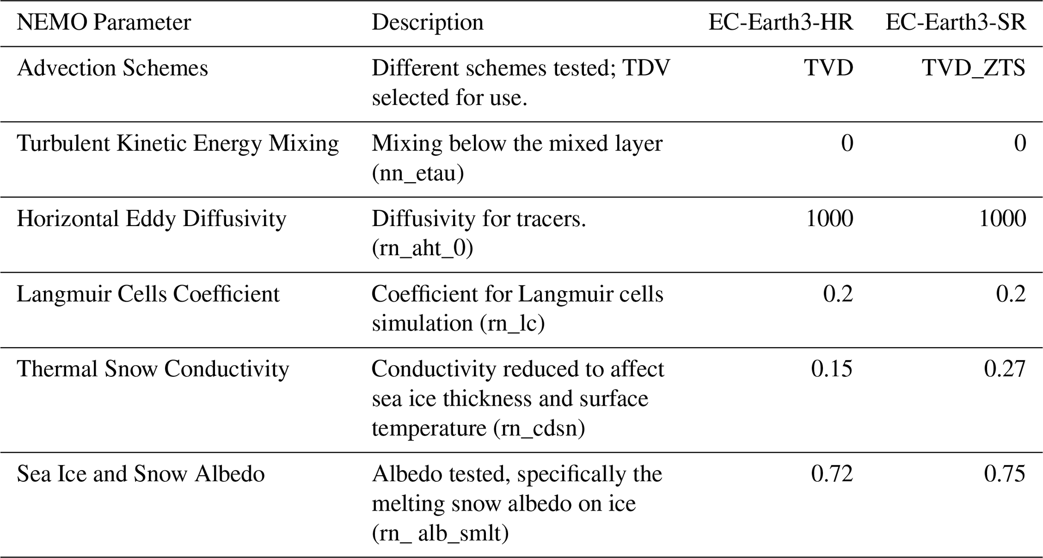
The parameters tested during the tuning are listed in Table 2, with the aim of reducing model biases. The selection of adjustable parameters follows earlier EC-Earth configurations, including EC-Earth3-SR (Döscher et al., 2022) and EC-Earth3P-HR in its second configuration (Haarsma et al., 2020). The evaluation of the different tuning options was based on quantitative diagnostics and climatological bias assessments. Global-mean and map-level comparisons of key variables were used to assess the overall differences relative to observational datasets and reanalysis products. We selected the tuning choices that, overall, reduced the model biases, as discussed below. With regards to the performance of the different advection schemes, we tested different advection schemes, including the Upstream-Biased Scheme (UBS) and, Total Variations Diminishing (TVD) approach. The UBS configuration showed a persistent warming drift in the global ocean temperature (100–1000 m) and surface heat fluxes that did not stabilise even after more than 130 years, while the TVD simulations showed a marked slowdown of drift and approached a quasi-steady state after about 60 years. The TVD scheme was therefore selected based on its long-term stability rather than on computational cost.

The turbulent kinetic energy (TKE) mixing below the mixed layer was set to zero (nn_etau = 0), as in EC-Earth3-SR (Döscher et al., 2022), which would otherwise lead to a significant reduction in AMOC. The tuning target was an observed AMOC strength in the range 17–18 Sv, consistent with RAPID estimates at 26.5° N (Smeed et al., 2018). It should be emphasized that this choice was not driven by the AMOC alone. Switching to nn_etau = 1 did not improve the overall coupled climate in EC-Earth3-HR, and sensitivity experiments with nn_etau = 0 produced preferable large-scale SST and sea-ice patterns in the North Atlantic–Arctic sector. With regard to the horizontal eddy diffusivity of tracers, the lateral mixing coefficient (rn_aht) was adjusted to a constant value of 1000 m² s⁻¹ same as in EC-Earth-SR, but in contrast to 300 m² s⁻¹ in the EC-Earth3P-HR configuration. Sensitivity experiments showed that rn_aht_0 = 1000 m² s⁻¹ yields a stronger AMOC and deeper Labrador Sea convection than rn_aht_0 = 300 m² s⁻¹ , with an overall improved North Atlantic–Arctic surface climate. For the lateral momentum mixing, EC-Earth-HR employs 2D-varying bilaplacian eddy viscosity with the reference value at the Equator of − 6.4 ×10¹¹ m⁴ s⁻¹, whereas EC-Earth-SR uses a 3D-varying Laplacian eddy viscosity with the reference value of 2 ×10⁴ m² s⁻¹. We set the background vertical mixing parameters to 10⁻⁴ and 10⁻⁵ m² s⁻¹ for the vertical eddy viscosity and diffusivity, respectively, compared with 1.2 $\times {\mathrm{10}}^{-\mathrm{4}}$ and 1.2 $\times {\mathrm{10}}^{-\mathrm{5}}$ m² s⁻¹ in EC-Earth-SR.

The Langmuir cell coefficients were maintained at 0.2, in accordance with EC-Earth3-SR and EC-Earth3P-HR. The thermal conductivity of snow (rn_cdsn) was reduced to 0.15 W m⁻¹ K⁻¹, in comparison to 0.27 W m⁻¹ K⁻¹ in EC-Earth3-SR and to 0.40 W m⁻¹ K⁻¹ in EC-Earth3P-HR, resulting in thinner sea ice and higher surface skin temperatures. The albedo of sea ice and snow on ice was adjusted, specifically the melting snow albedo on ice (rn_alb_smlt), to 0.72 (from 0.75). This resulted in earlier melting of snow on ice and reduced ice thickness in summer.

Table 1 Atmospheric tuning parameters changed in T511L91 compared to T255L91.

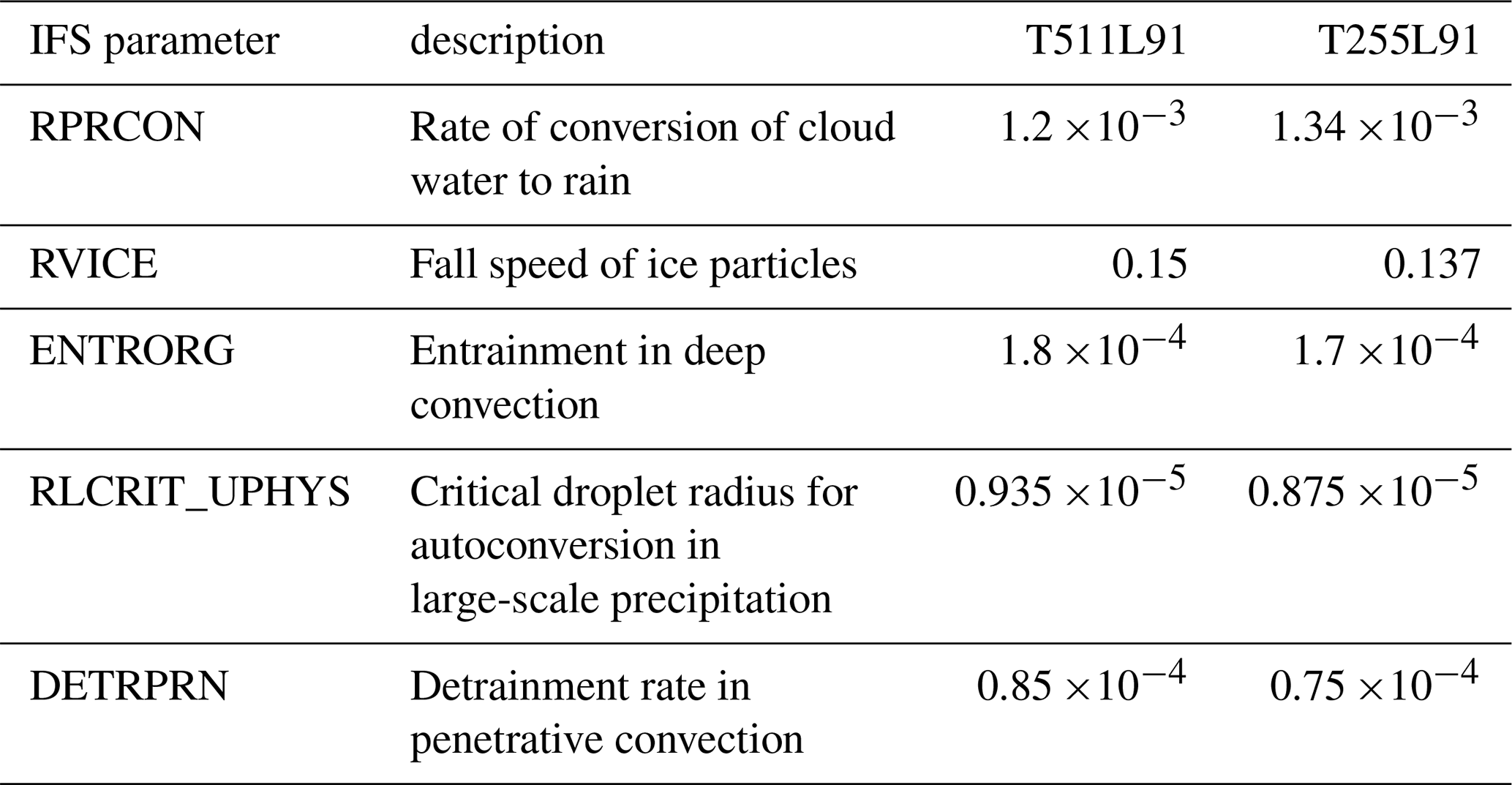
Table 2 Ocean parameters tested during tuning and their final values.

Starting from the pre-industrial (PI) control run, we initiated a historical simulation spanning from 1850 to 2014. This simulation was extended with a future projection that continued until the year 2100, following the SSP2-4.5 emission scenario. The SSP2-4.5 scenario was selected because it is currently the CMIP6-Tier 1 scenario most closely aligned with CO₂ concentrations that could be reached following “The Stated Policies Scenario” (STEPS), which provides an outlook based on the latest policy settings, including energy, climate and related industrial policies (IEA, 2023). In addition to the historical and future simulations, we also conducted a simulation with a 1 % annual CO₂ increase starting from the PI control run. Despite the inclusion of this scenario, our study primarily focuses on the outcomes from the historical and future simulations. The results from these simulations contribute to understanding the potential impacts of climate change under moderate mitigation strategies and provide valuable insights into the trajectory of global climate dynamics over the next century.

3 General evaluation of the model

As this is the first article to use the official EC-Earth3-HR version, we begin by providing an overview of the model's performance and biases, focusing on key variables related to the atmosphere, ocean, and sea ice. This overview sets the stage for a more detailed analysis of the North Atlantic and Arctic regions.

3.1 Mean historical climate

Figure 1 presents a comparison of the temperature time series of the EC-Earth3-HR model (in black) with reanalyses and observational estimates (in blue or green). Furthermore, the results from the 24-member ensemble of the EC-Earth3-SR model for CMIP6 are presented as a grey shaded envelope for reference. The global mean near-surface temperature (TAS) of the high-resolution model is in good agreement with that of ERA5 (Hersbach et al., 2020), while the EC-Earth3-SR ensemble consistently displays a higher temperature (Fig. 1a). The high-resolution model better depicts the observed warming since 1950, while the EC-Earth3-SR displays a trend stronger than that of ERA5. The situation changes when the data are separated into land and ocean categories. Both model resolutions, exhibit temperatures lower than that observed in both the CRU (Harris et al., 2020) and ERA5 datasets over land (Fig. 1b). EC-Earth3-HR remains within the EC-Earth3-SR ensemble, but it is on the cold side. When compared to the CRU or ERA5 data, the EC-Earth3-HR model produces a temperature approximately 2° K lower than the observed values. In contrast to land temperature, the global mean SST from the EC-Earth3-HR model is close to the value of the HadISST data set (Rayner et al., 2003) while the SST in the EC-Earth3-SR ensemble is significantly warmer (Fig. 1c).

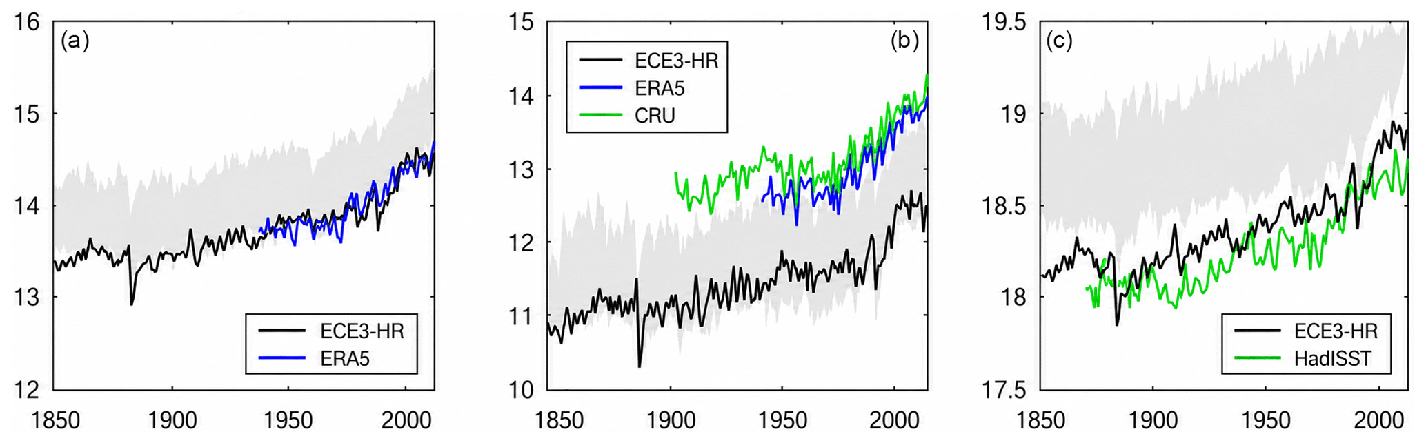
Figure 1 Time series of surface air temperature (TAS, °C) and sea surface temperature (SST, °C) from EC-Earth3-HR (black), ERA5 reanalysis (blue), CRU over land (green), and HadISST over ocean (green) for the historical period. The full range of the EC-Earth3-SR CMIP6 historical ensemble is shown as a grey shaded area. Panels show: (a) global mean TAS, (b) global mean TAS over land (excluding Antarctica) and (c) global mean SST.

The present-day annual mean near-surface temperature (TAS), total precipitations (pr) and sea level pressure (psl) are compared with ERA5 over the period 1980–2010 in Fig. 2. All the parameters are regridded to 0.5° × 0.5° using bicubic interpolation before comparison. Compared to ERA5, EC-Earth3-HR is colder over the Arctic and warmer over Antarctica and the surrounding ocean areas. The extent to which EC-Earth3-HR exhibits a cold bias in the Arctic remains unclear, given that ERA5 itself has a warm bias in the region (Tian et al., 2024). EC-Earth3-HR is slightly colder over most of the continents, with the cold biases having a similar distribution pattern to EC-Earth3-SR (Döscher et al., 2022). However, there are also noticeable warm biases over the Siberian and the Greenland adjacent ocean regions. The Southern upwelling regions, along the South American and African coasts, are better simulated in EC-Earth3-HR compared to EC-Earth3-SR with less warm bias. In addition, the warm bias over Antarctica and the Southern Ocean has been previously attributed to the parametrization of shortwave cloud radiative effects in climate models (Hyder et al., 2018; Dösher et al., 2022). Similar to EC-Earth3-SR, the spatial precipitation pattern is well captured in EC-Earth3-HR. However, the simulated double Intertropical Convergence Zone (ITCZ) is still displaced to the south, likely due to the persistent strong warm bias over the Southern Ocean (Hwang and Frierson, 2013; Döscher et al., 2022). The wet and dry biases in EC-Earth3-SR have been slightly improved in EC-Earth3-HR, particularly over the tropical Pacific Ocean. For PSL, EC-Earth3-HR shows similar spatial patterns as ERA5. PSL biases are relatively small in tropical and mid-latitude areas but are more pronounced over the Arctic and Antarctic. The substantial bias in the Southern Ocean is primarily due to anomalous warming in our model simulation. In general, EC-Earth3-HR reproduces a reasonable mean climate. TAS generally exhibits a bias of less than 1–2 K over most continents. Regarding precipitation, the bias remains below 0.5 mm d⁻¹ over most land areas, except in the Amazon region. The improvements may result from a refined representation of orography.

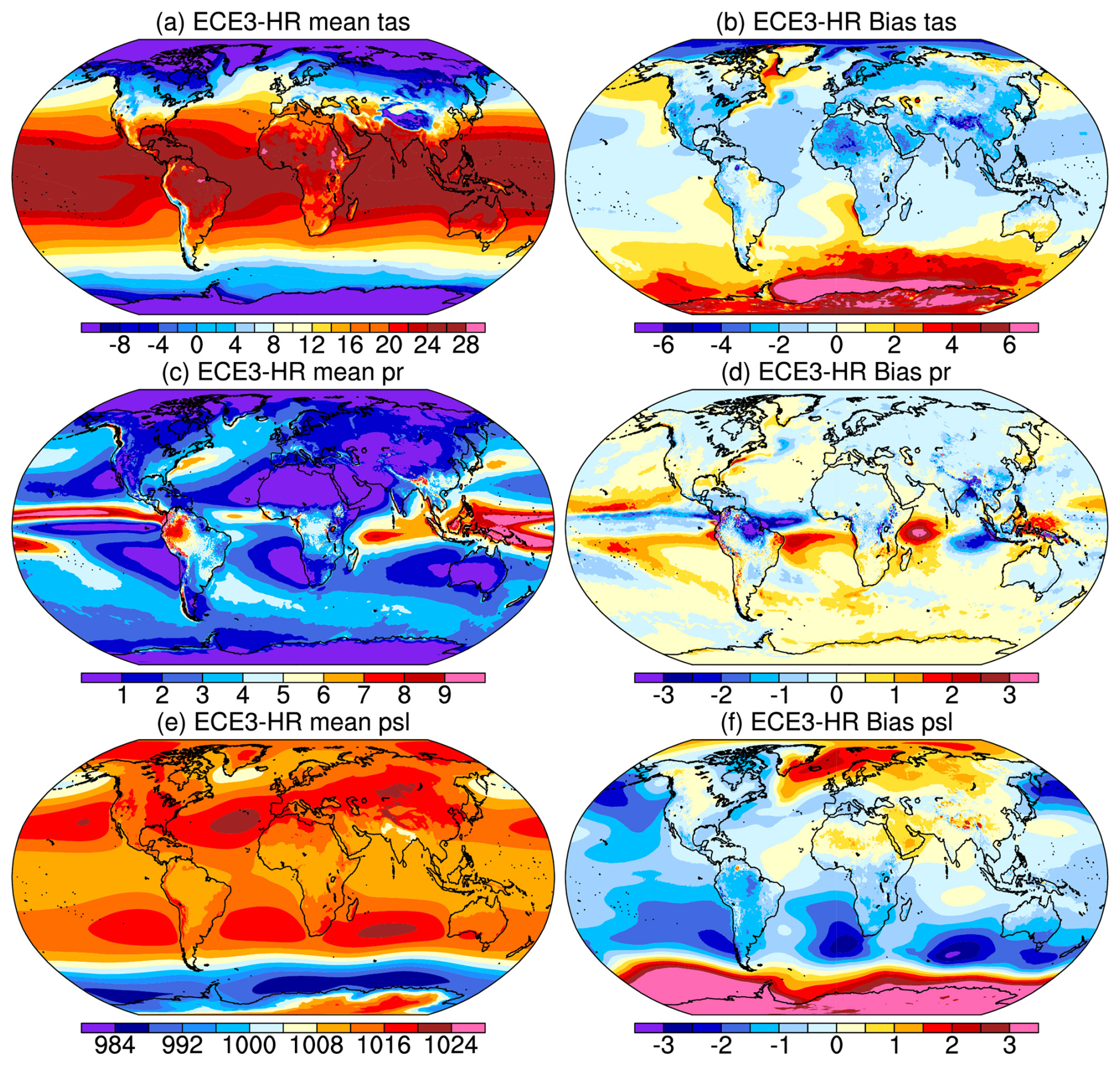
Figure 2 Annual mean (a) near-surface temperature (TAS, °C), (c) total precipitations (pr, mm d⁻¹) and (e) sea level pressure (psl, hPa) simulated by EC-Earth3-HR for the period 1980–2010, and (b), (d), (f) their respective biases compared to ERA5.

There are large regional differences in sea ice concentration between EC-Earth3-HR and satellite observations, and these differences are generally similar to those observed in EC-Earth3-SR (Fig. 3a, b). In March, the model overestimates sea ice concentration in the Greenland-Iceland-Norway (GIN) and Barents Seas, and underestimates it in the Labrador and Bering Seas. The largest discrepancy between EC-Earth3-HR and EC-Earth3-SR (see Fig. 11 in Döscher et al., 2022) occurs in the sea ice coverage over the Labrador Sea likely due to the difference in fluxes through Canadian Arctic Archipelago (Karami et al., 2021). In September, the sea ice concentration is underestimated in the Kara, Laptev and Chukchi Seas, while exhibiting an overestimation at the ice margins. Different regions of the Arctic are losing sea ice at different rates. The trend in sea ice concentration (% per decade) from 1980–2010 compared to observations, shows notable regional discrepancies, particularly in the Beaufort and Chukchi seas (Fig. A2).

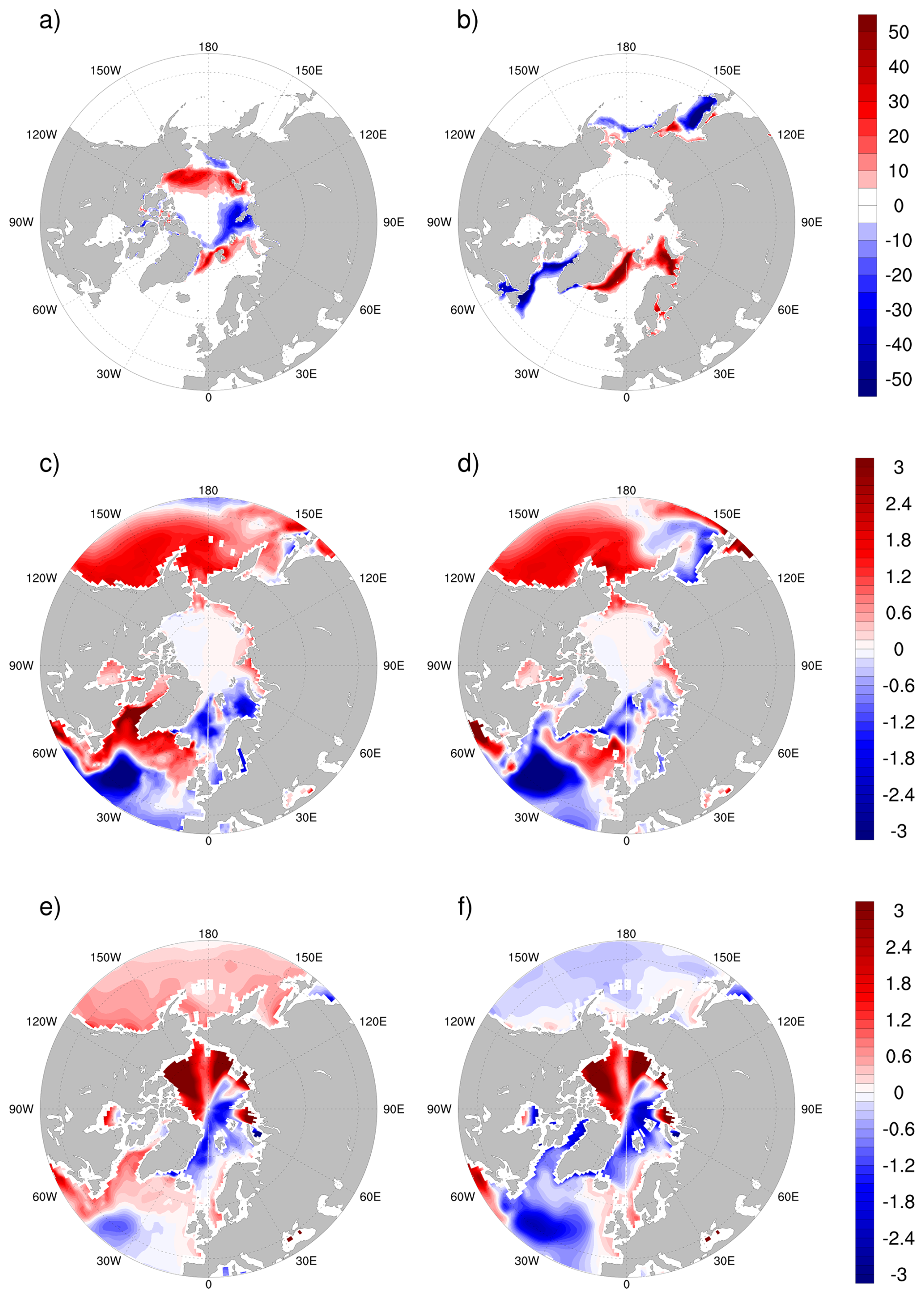
Figure 3 Mean biases over 1980–2010. (a, b) Difference in sea ice concentration (%) between the EC-Earth3-HR model and satellite observations for September and March, respectively. (c, d) Annual mean sea surface temperature (SST; °C) bias in EC-Earth3-HR and the EC-Earth3-SR ensemble mean relative to HadISST, respectively. (e, f) Sea surface salinity (SSS; psu) bias in EC-Earth3-HR and the EC-Earth3-SR ensemble mean compared to WOA18, respectively.

Regarding SST bias, Fig. 3c, d illustrates the bias between EC-Earth3-HR and HadISST, and compares it to the bias between the ensemble mean of EC-Earth3-SR and HadISST. The patterns are generally similar in both resolutions. The largest biases occur along the east coast of North America and in the southern part of the subpolar gyre and reach up to around ± 5 °C. These biases are typical of standard resolution climate models where the Gulf Stream extends too far to the north along the North American coast and the North Atlantic Current goes too zonally across the North Atlantic, thus allowing the subpolar gyre to extend too far to the south. EC-Earth3-HR shows a different bias in the Gulf Stream region along the North American east coast. This is linked to changes in the position of the Gulf Stream and the North Atlantic Current in the high-resolution version. On the other hand, EC-Earth3-HR shows a positive bias in the Labrador Sea, mainly due less sea ice in this region. Also in the subtropical North Atlantic, a slightly larger cold bias is visible in EC-Earth3-HR compared to EC-Earth3-SR. It should be noted that the biases observed in individual EC-Earth3-SR simulations are generally more pronounced than those evident in the ensemble mean that is used here as comparison. The bias pattern of SSS (Fig. 3e, f) in EC-Earth3-HR is comparable to that of the SST bias. In most areas with a warm bias (Labrador Sea, along North american coast), EC-Earth3-HR simulates too high salinity compared to the observational based climatology while in the cold-bias regions, salinity tends to be too low. As previously seen for the SST-biases, the SSS-biases in EC-Earth3-HR are smaller in the Gulf-Stream-North Atlantic Current region than in EC-Earth3-SR. In contrast to EC-Earth3-HR, EC-Earth3-SR also simulates too low salinity in the entire Labrador Sea and Baffin-Bay area. Overall, compared to EC-Earth3-SR, the improvements strongly depend on the geographical region. The enhanced horizontal resolution does not consistently yield improvements across all processes due to inherent limitations in parameterization (Fosser et al., 2015).

3.2 Climate variability modes

Figure 4 presents a comparison of the NAO patterns in EC-Earth3-HR with those in EC-Earth-SR and in ERA5. Both EC-Earth3-versions exhibit similarities in the pattern and location of the high and low centers, closely aligning with the reference ERA5 plot. However, EC-Earth3-HR underestimates the intensity of both the positive and negative pressure centers, which are located in the subtropical and North Atlantic regions, respectively.

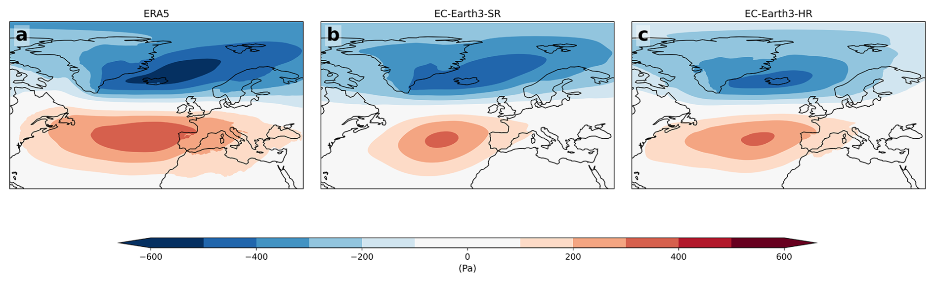
Figure 4 Regression of sea level pressure anomalies onto the NAO index during winter (December–February) for ERA5 reanalysis (a), EC-Earth3-SR member 1 (b), and EC-Earth3-HR (c). The NAO index is defined as the difference in area-averaged SLP between the Azores (31.5–24.5° W, 36.5–40° N) and Iceland (25–13° W, 63–67° N), following Fereday et al. (2020) and Fuentes-Franco et al. (2023).

We calculated the regression of the Niño 3.4 index (5° N–5° S, 170° W–120° W) on sea level pressure for the winter season (December to February, DJF) using ERA5 reanalysis data and the EC-Earth3-SR and EC-Earth3-HR models (Fig. 5a, d, g). The results reveal a positive Pacific North American (PNA) like pattern characterized by an intensified low-pressure system over the Aleutian region and lower pressure over the eastern United States. This low-pressure system extends along the North American east coast into the central North Atlantic Ocean, while higher pressure is observed over and between Iceland and Scandinavia, resembling a negative phase of the NAO. Both EC-Earth3-SR and EC-Earth3-HR show strong similarity to ERA5, with the high-resolution model exhibiting higher intensity and greater resemblance to ERA5. Moreover, EC-Earth3-SR shows weaker surface pressure anomalies, likely due to a slightly weaker ENSO intensity compared to EC-Earth3-HR. Therefore, EC-Earth3-HR represents a clear improvement in capturing the ENSO-SLP response. The SST Niño 3.4 index anomaly spectrum exhibits dominant variability in the 4–6 year range (Fig. 5c, f, i). EC-Earth3-SR captures the most significant frequencies similarly to HadISST, while EC-Earth3-HR displays higher intensity at the 4-year frequency.

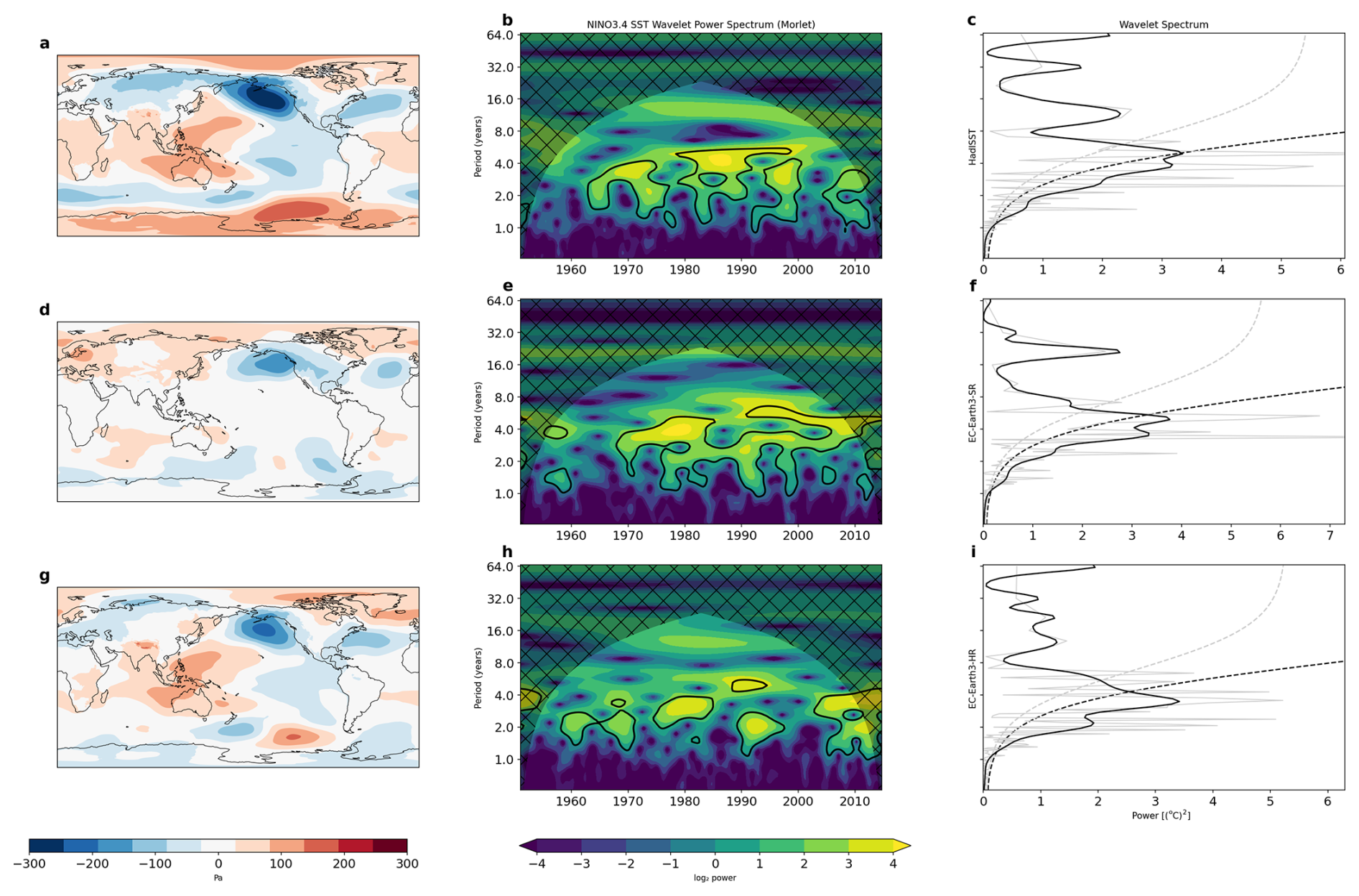
Figure 5 Niño 3.4 analyses during winter (DJF): regression of sea level pressure anomalies onto the Niño 3.4 SST index (left column), wavelet power spectra (middle column), and global wavelet power spectra (right column). Rows correspond to different datasets: ERA5 (top row: a–c), EC-Earth3-SR member 1 (middle row: d–f), and EC-Earth3-HR (bottom row: g–i). The Niño 3.4 index is defined as the average SST over 5° N–5° S, 170° W–120° W. Power spectra are computed over 1951–2014 using 3-month means for December–February.

4 Projected changes in the Arctic and North Atlantic Oceans under the SSP2-4.5 scenario

4.1 Changes in the Arctic sea ice and temperature in future projections

Figure 6a shows the time series of September Arctic sea ice area from 1850 to 2100 for EC-Earth3-HR (in black). In addition, the EC-Earth3-SR CMIP6 ensemble is shown as a grey shaded envelope, with the ensemble mean in red. The EC-Earth3-HR simulation slightly underestimates the Arctic sea ice area compared to the sea ice reconstruction of Walsh et al. (2019; in blue) and the OSI SAF satellite observations (Lavergne et al., 2019; in green). However, it captures the rapid observed decline of sea ice between 1995 and 2010. While these results are based on a single-member simulation, making it difficult to draw firm conclusions, it still highlights the ability of the model to simulate realistic, rapid sea ice loss. The sea ice area shows a significant downward trend, with a marked reduction starting around 2000. From 2040, the Arctic becomes nearly ice-free in September, with sea ice area consistently below 1 million km², reaching fully ice-free conditions by 2050 under the SSP2-4.5 scenario. The projected timing of an ice-free Arctic varies widely across models, reflecting large uncertainty. In CMIP6, the multimodel ensemble mean projects September ice-free conditions by 2050 under the high-emission scenario SSP5-8.5, with delayed occurrences for SSP2-4.5 (Notz and SIMIP Community, 2020). However, both Docquier and Koenigk (2021) and Selivanova et al. (2024) project an ice-free Arctic before 2050 based on observationally constrained model projections, consistent with our EC-Earth3-HR estimate.

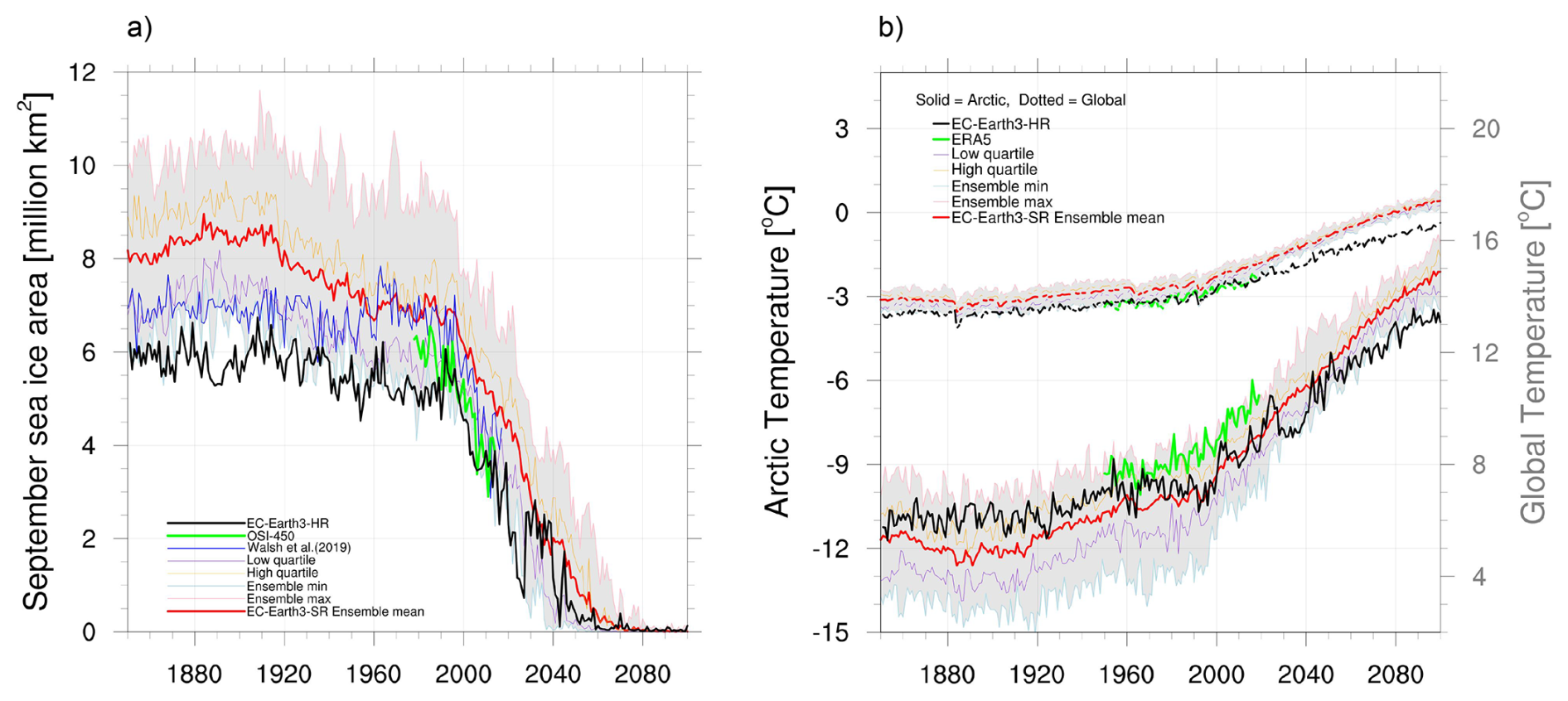
Figure 6 (a) September Arctic sea ice area (million km²) from EC-Earth3-HR (black), the 14-member EC-Earth3-SR ensemble (red is for the ensemble mean, and grey shading indicates the ensemble spread including minimum, maximum, and interquartile range), satellite observations OSI-450 (green; OSI SAF, 2017) and sea ice reconstruction of Walsh et al. (2019; blue). (b) Annual mean surface air temperature (°C) over the Arctic (solid lines) and the globe (dotted lines) for EC-Earth3-HR (black), ERA5 reanalysis (green), and the EC-Earth3-SR ensemble (red is for the ensemble mean, and grey shading indicates the ensemble spread). Historical simulations cover 1850–2014, with projections from 2015–2100 under the SSP2-4.5 scenario.

The decline in sea ice is closely linked to rising Arctic temperature, which is increasing faster than the global average – a phenomenon known as Arctic amplification (Holland and Landrum, 2021). We find that the annual mean global surface temperature anomaly and the Arctic-averaged temperature anomaly (both relative to modeled pre-industrial values) exhibit distinct warming trends, as expected (Fig. 6b). In EC-Earth3-HR, the global mean temperature anomaly (in dashed black) reaches 1.5 °C by around 2023, 2 °C by 2045, and 3.2 °C by 2100, while the Arctic experiences much stronger warming, with an anomaly of 2 °C by around 2000, accelerating to 4 °C by 2040 and 7 °C by 2100 (in solid black; Fig. 6b). The EC-Earth3-SR ensemble confirms this pattern but shows stronger global and Arctic warming than EC-Earth3-HR throughout the 21st century.

To illustrate the projected spatial sea ice changes, we compare the March sea ice concentration for the 2070–2100 mean with the 1980–2010 mean (Fig. A3). Substantial declines are observed, particularly in the Barents, Greenland and Bering Seas. As September sea ice is projected to disappear by mid-century, we focus instead on the trend from 2020 to 2050 for this month. The trend in September sea ice concentration (% per decade) shows that sea ice loss is occurring at different rates in different Arctic regions with particularly strong reductions in the Central Arctic Basin and the Canadian Arctic Archipelago. These spatial variations indicate that sea ice loss will be more pronounced in certain areas in the coming decades.

4.2 Projected changes in North Atlantic Ocean properties

The spatial distribution of ocean temperature and salinity, through its influence on the zonal and meridional density gradients, is an important driver of ocean circulation changes. Furthermore, the distribution of North Atlantic SST can impact the large scale atmospheric circulation (e.g. Gastineau and Frankignoul, 2015). The projected change in SST, comparing the 2070–2100 mean to the 1980–2010 mean, shows moderate to strong warming (Fig. 7a), though this warming is not uniform across all regions. The most pronounced warming occurs where the winter sea ice edge has shrunk, particularly in the Greenland Sea. In comparison, EC-Earth3-SR (Fig. A4) exhibits more pronounced warming than EC-Earth3-HR, with a broader extent across the entire Nordic Seas. EC-Earth3-SR also shows considerably greater warming in the Labrador Sea and the subpolar gyre. This difference between the two model versions is partly due to the larger extent of sea ice in EC-Earth3-SR, which led to more significant sea ice reductions in these regions. The North Atlantic warming hole, a region characterized by no temperature increase in the eastern subpolar gyre (e.g., Liu et al., 2020), is also evident in Fig. 7a, where a moderate surface cooling anomaly can be seen compared to the historical period. This cooling pattern has been linked to the weakening of the AMOC (Drijfhout et al., 2012). Looking at the region of the warming hole in the deeper layers, we find that the cooling is more present in the upper few hundred meters (not shown).

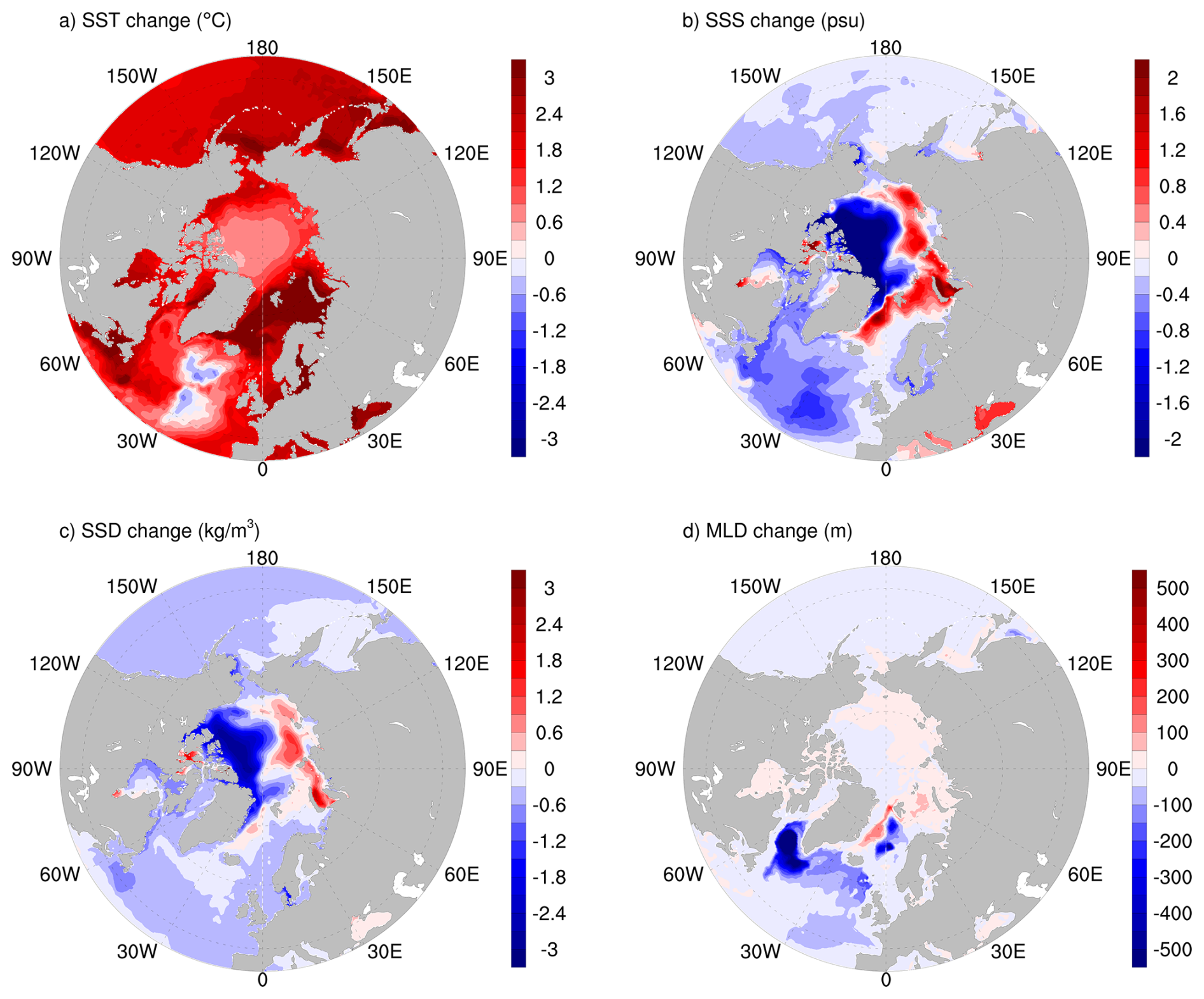
Figure 7 Differences between the 2070–2100 and 1980–2010 periods under the SSP2-4.5 scenario in EC-Earth3-HR for: (a) annual mean sea surface temperature (SST, °C); (b) annual mean sea surface salinity (SSS, psu); (c) winter mean (JFM) sea surface density (SSD, kg m⁻³); (d) winter mean (JFM) mixed layer depth (MLD, m). All figures are shown for 40° N northward.

The projected changes in SSS in EC-Earth3-HR (Fig. 7b) are dominated by decreasing salinity in mid and high latitudes, with exceptions in the Greenland Sea and eastern Arctic, where salinity increases. The freshening is most pronounced in the Beaufort Gyre and western Arctic. Conversely, salinification in the Greenland Sea and eastern Arctic is also projected. Salinity changes may arise from changes in Arctic circulation (Karami et al., 2021), river runoff and precipitation, and increased advection of Atlantic Water into the region, but the underlying mechanisms remain uncertain and require further investigation beyond the scope of this study. EC-Earth3-SR exhibits an overall similar pattern of SSS change (Fig. A4). This model agreement supports the robustness of the projected SSS changes across resolutions, despite model uncertainties.

The distribution of water masses in the North Atlantic strongly influences mixing and deep-water formation, particularly in the core convection regions of the Labrador, Irminger, and Greenland Sea. To better understand these changes, we analyze sea surface density (SSD) and mixed layer depth (MLD) for the winter season. The SSD anomaly pattern resembles salinity over the Arctic, with positive anomaly in the eastern Arctic and negative anomaly in the western Arctic (Fig. 7c). This density contrast reflects the dominance of salinity-driven changes in the surface Arctic Ocean. Over the North Atlantic, both SST and SSS contribute to density changes, though SST plays a dominant role in driving SSD distribution over the central to eastern Atlantic (east of 30° W). The influence of SST is particularly evident in areas with strong surface warming, which reduces density and vertical mixing. The winter mixed layer depth serves as a proxy for the location and depth of deep convection, and the MLD analysis reveals a clear reduction of its intensity in the Labrador, Irminger, and Greenland Seas (Fig. 7d). This is spatially consistent with SSD reductions in these regions that has led to increased stratification and weakened convective mixing. These patterns are particularly evident in the Labrador and Greenland Seas, indicating that there may be regionally distinct drivers of stratification. In the former region, there is a combination of warming and freshwater accumulation; in the latter region, warming is the predominant factor. This decrease in MLD, driven by density changes in the North Atlantic, is consistent with reduced deep-water formation and weaker AMOC in line with the established sensitivity of overturning strength to high-latitude density and buoyancy forcing (Buckley and Marshall, 2016). These changes in the AMOC, including its present-day structure and projected future weakening, are discussed in detail below.

4.3 Changes in the AMOC

AMOC involves the northward flow of warm, salty water in the upper Atlantic Ocean, which cools and sinks at high latitudes, driving a southward flow of cold, dense water in the deeper layers (Buckley and Marshall, 2016). The AMOC stream function reveals the typical overturning circulation (Fig. 8) and, for the 1980–2010 mean, has a peak transport of more than 18 Sv occurring at a depth of approximately 1000 m. Compared to the ensemble mean of EC-Earth3-SR used in CMIP6 (Fig. 15 in Döscher et al., 2022), EC-Earth3-HR simulates a slightly stronger AMOC. The AMOC stream function is projected to weaken in the future, with the mean for the period 2070–2100 showing a decline of 5.6 Sv relative to the 1980–2010 mean (Fig. 8c). This AMOC weakening is consistent with the reductions in density and MLD discussed earlier. The projected structure of the overturning cell also exhibits a shallower and less extensive circulation, reflecting disruptions to key driving mechanisms, such as dense water formation. This reduction of AMOC under future climate scenarios aligns with CMIP6 model projections (Bellomo et al., 2021).

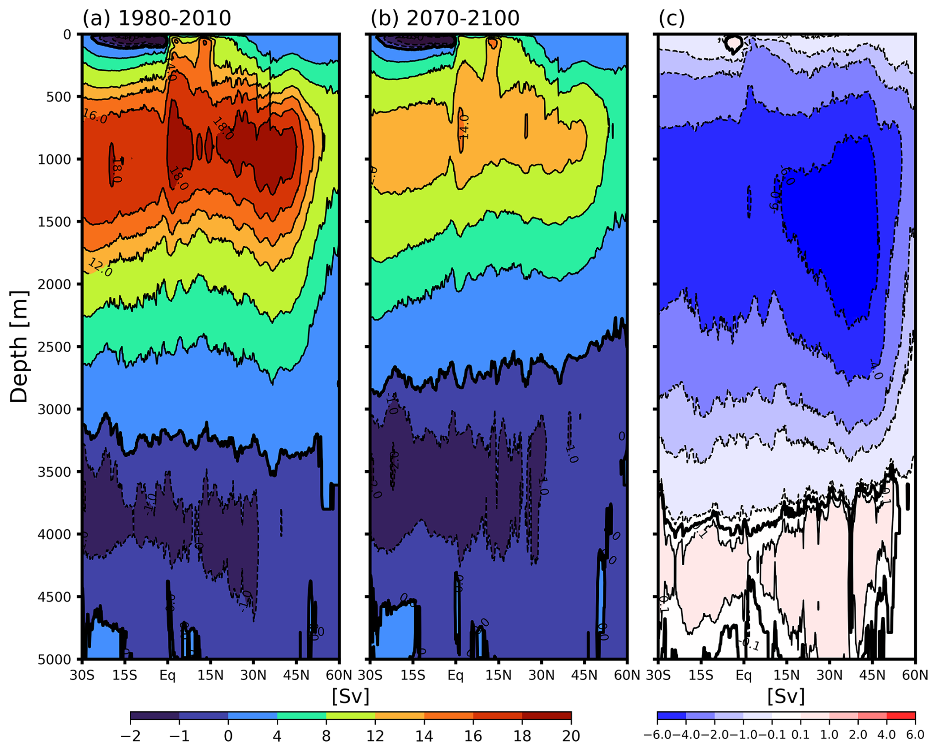
Figure 8 AMOC stream function (Sv) in the depth-latitude space for EC-Earth3-HR, averaged over 1980–2010 (a) and 2070–2100 (b) and the difference between the two periods (c).

The time series of the AMOC index, calculated as the maximum volume transport stream function between 20 and 40° N and 800–1100 m depth (Fig. 9a), is slightly higher than the observations from the RAPID-MOCHA array (Smeed et al., 2018). However, the model captures variability of comparable amplitude to observations. The EC-Earth3-HR simulation closely follows the ensemble maximum values of EC-Earth3-SR until around year 2000 but remains close to the ensemble mean after that. The AMOC index shows a clear reduction in the 21st century, decreasing from around 21 to 13 Sv, which represents a reduction of approximately 39 %. This is within the range of the findings of Weijer et al. (2020), where they estimated a decline of 6 to 8 Sv (34 %–45 %) of AMOC in CMIP6 models, after selecting the models constrained with RAPID observations.

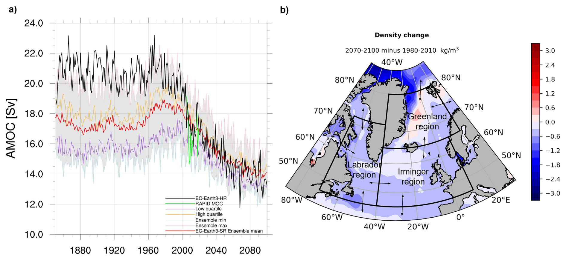
Figure 9 (a) Annual-mean AMOC strength (maximum overturning stream function between 20–40° N at 800–1100 m depth) from 1850 to 2100 in EC-Earth3-HR (black), the 14-member EC-Earth3-SR ensemble (red is the ensemble mean, and grey shading indicates ensemble spread including minimum, maximum, and interquartile range), and RAPID-MOCHA observations (Smeed et al., 2018; green). (b) Winter mean (JFM) surface density change (kg m⁻³ decade) between the 2070–2100 and 1980–2010 periods in the North Atlantic showing the three analysis regions used in Sect. 4.4: the Greenland, Irminger, and Labrador regions. These polygons represent extended areas encompassing and surrounding the respective seas. Arrows indicate the sections where inflows and outflows are calculated.

4.4 Changes in stratification, convection, and deep-water formation contributing to AMOC weakening

The North Atlantic plays a critical role in AMOC dynamics through deep convection, the formation of dense water masses, and their subsequent southward transport. These processes primarily occur in three key regions: the Labrador Sea, the Irminger Sea, and the Greenland Sea. In Fig. 9b, these regions are indicated by polygons defining the areas used in the analysis below. To assess changes in these regions in EC-Earth3-HR, we first examine the time–depth evolution of density (Fig. 10), which highlights long-term changes in stratification and isopycnal structure. This analysis is complemented by two indices: one representing convection and the other quantifying the rate of deep water formation.

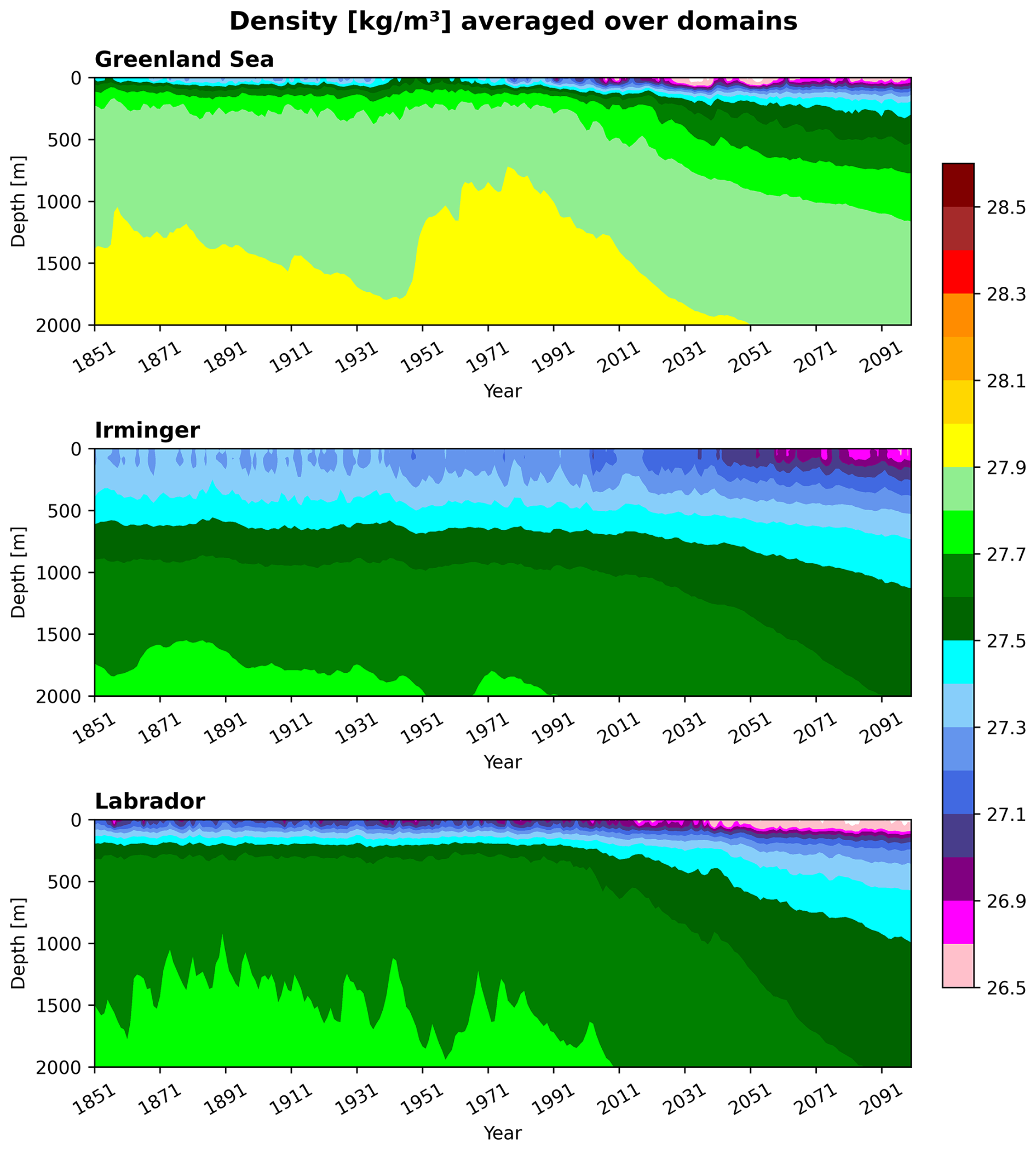
Figure 10 Time–depth evolution of winter (JFM) density (kg m⁻³) averaged over the Greenland, Irminger, and Labrador regions from 1850 to 2100. Color shading indicates isopycnal structure. The regions correspond to polygons shown in Fig. 9b.

Increased stratification

Figure 10 shows the evolution of winter (JFM) density (kg m⁻³) profiles averaged over the Greenland, Irminger, and Labrador regions (shown as polygons in Fig. 9b) from 1851 to 2100, highlighting long-term changes in vertical stratification in the North Atlantic. In all three regions, stratification becomes increasingly pronounced over time, particularly in Greenland and Labrador after the late 20th century, as lighter density classes expand and thicken in the upper ocean. These trends reflect enhanced surface stratification, which inhibits vertical mixing and suppresses deep convection, consistent with changes in surface forcing and water mass transformation under climate change. In the Greenland Sea, the upper ocean shows a marked increase in the thickness of low-density layers, especially after the year 2000, while the denser water masses at depth have moved deeper and become less prominent. In the Irminger region, lighter densities gradually occupy a greater proportion of the upper 1000 m over time. In the Labrador region, a similar pattern emerges, with a pronounced thickening of lighter density classes in the upper ocean and a corresponding reduction in the volume of dense water at depth.

Weakened convection

A common index for diagnosing convection is the MLD, but it only provides depth information and does not capture the spatial extent of convection. Here, we use the Deep Mixed Volume (DMV) index (Brodeau and Koenigk, 2016), which quantifies the total volume of water involved in deep convection by integrating both the depth and horizontal extent of the mixed layer below a reference depth. It thus offers a more comprehensive measure of convection than MLD. Here, the DMV is computed for March over the Labrador, Irminger, and Greenland regions (shown as polygons in Fig. 9b), providing a volumetric measure of deep convection in these key areas. To compute the DMV, a reference depth must be specified. We follow the definition of deep convection adopted by Brodeau and Koenigk (2016), building on Marshall and Schott (1999), which assumes that convection contributes most directly to the AMOC when it reaches either the depth of the southward-flowing branch (∼ 1000 m) or the depth of the overflow sills (∼ 700 m). Accordingly, Brodeau and Koenigk (2016) used an observation-based reference depth of 1000 m for the Labrador Sea and a shallower threshold of 700 m for the Greenland Sea. For the Irminger Sea, given its location, we use the same reference depth as for the Labrador Sea. While mixed layer in the Irminger Sea is generally shallower than 1000 m, deep convection events exceeding this depth have been reported (Våge et al., 2009; Piron et al., 2017) and are also simulated in EC-Earth3-HR. We acknowledge that the diagnosed DMV depends on the selected reference depth and using a 1000 m threshold in the Irminger Sea may underestimate the absolute DMV. For consistency across basins and to focus on the deepest convection events, we retain this threshold but also repeat the analysis using a shallower reference depth (500 m; Fig. A5).

The DMV in EC-Earth3-HR shows notable internal variability across all three basins until the late twentieth century, followed by a marked and persistent decline (Fig. 11). The Labrador Sea shows the largest DMV values, with a significant decline after 1980, approaching near-zero values by around 2050. The Greenland Sea also shows a significant decline after 1980, reaching near-zero values earlier, around 2020. The Irminger Sea has smaller DMV values than the Labrador and Greenland Seas for the 1000 m criterion, and shows a more gradual reduction through the twenty-first century. Using a shallower threshold increases the absolute DMV values, but does not change the temporal evolution or the long-term declining tendency. This suggests that the qualitative behavior of DMV is not sensitive to the choice of reference depth (Fig. A5). The reduction in DMV across the three convection regions is consistent with the projected slowdown of AMOC, which also declines markedly after 1980 (Fig. 9).

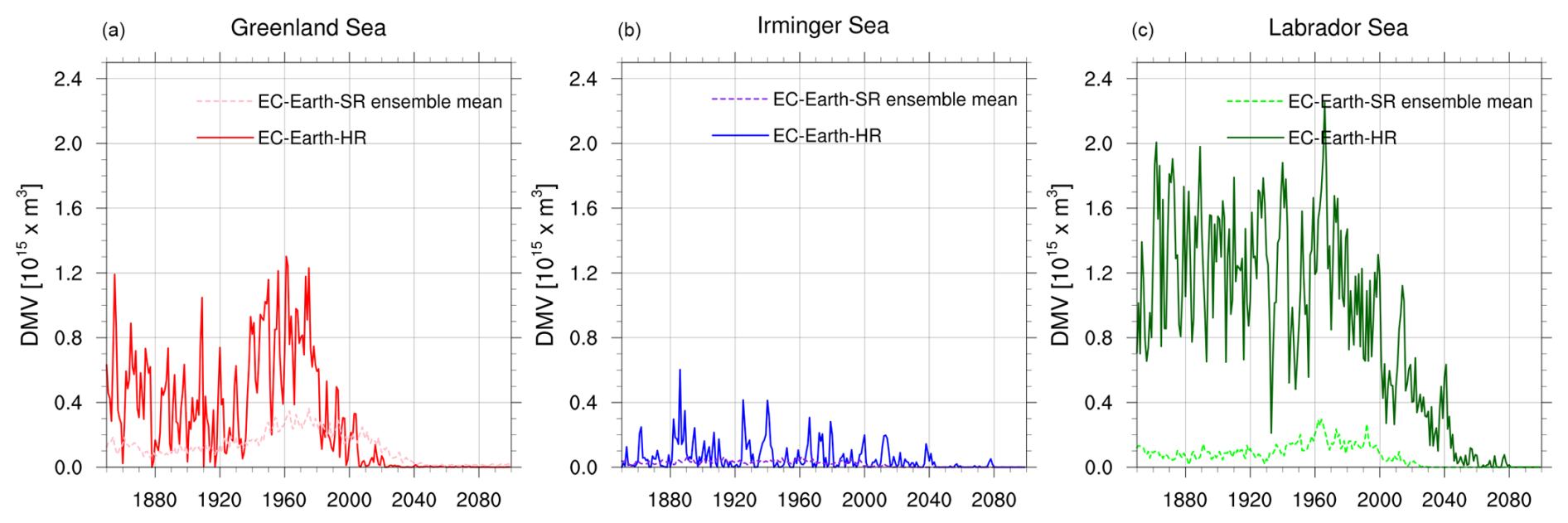
Figure 11 Deep Mixed Volume (DMV) for March in the Greenland Sea (a), Irminger Sea (b), and Labrador Sea (c), from historical and SSP2-4.5 simulations of EC-Earth3-HR (thick lines) and the ensemble mean of EC-Earth3-SR simulations (dashed lines). We chose the reference depth of 1000 m for the Labrador and Irminger Seas and 700 m for the Greenland Sea.

When compared to the DMV in EC-Earth3-SR, the DMV in EC-Earth3-HR is larger, in line with the findings of Koenigk et al. (2021), who reported an enhanced DMV with increasing resolution in HighResMIP models. This comparison uses identical reference depths in both model versions, as both configurations have similar depths of the major overflow sills and a comparable depth of maximum AMOC. In EC-Earth3-HR, convection in the Greenland Sea reaches near-zero values first, followed by the Labrador Sea after a delay of about two decades. In contrast, in EC-Earth3-SR, DMV declines earlier in the Labrador Sea and later in the Greenland Sea.

Reduced deep water formation

To complement the DMV, we introduce a volume-budget diagnostic of deep water formation (DWF) in the Labrador, Irminger, and Greenland Seas. This diagnostic is designed to quantify the regional contributions of these basins to the AMOC. Previous studies have characterized the spatial distribution of vertical mass transport and regional contributions to the AMOC using diagnostics based on vertical velocity fields (e.g., Katsman et al., 2018; Sayol et al., 2019). Here, we adopt an alternative approach, inferring these contributions from horizontal transports across gateway sections within a volume-budget framework. This yields a framework that does not rely on vertical velocity fields and is therefore applicable even to model output in which this variable is not archived.

For each region, we evaluate the net horizontal volume transport across lateral boundaries, separately considering an upper layer (from the surface to a common reference depth) and a lower layer (from that reference depth to the bottom), using the same reference depth across all regions and boundary sections (Fig. 12a). Given the diagnosed net horizontal inflow above the reference depth and the net horizontal outflow below it, the implied net downward volume transfer across the reference-depth surface that is required by volume conservation represents the DWF in each region. However, it is important to note that this should not be interpreted as a diapycnal water-mass transformation rate, because the locations where surface waters densify do not directly correspond to mean downwelling or dense-water export. Dense waters may form in one location, be advected along boundary currents, and sink elsewhere (Spall and Pickart, 2001; Katsman et al., 2018; Brüggemann and Katsman, 2019).

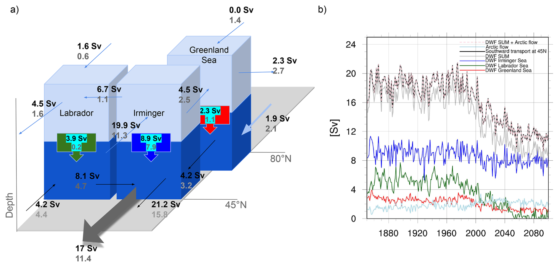
Figure 12 (a) Illustration of the regions used for DWF calculations in EC-Earth3-HR: blue thin arrows represent inflows and outflows in the upper layers, and black arrows indicate flows in the lower layers. Colored callouts with the downward arrows display DWF, with values in black corresponding to the 1980–2010 mean and numbers in grey to the 2070–2100 mean. The large grey arrow represents the net flow through 45° N, calculated as the sum of all DWFs and the deep inflow from the Arctic into the Greenland Sea. The thick blue arrow shows the deep outflow from the Arctic into the Greenland Sea. (b) Time series of southward deep transport at 45° N (black) and deep water formation (DWF) rates in the Irminger (blue), Labrador (green), and Greenland (red) seas, Arctic flow below 1000 m (light blue), together with sum of all DWFs (DWF SUM in grey) and DWF SUM plus deep Arctic flow (pink dashed). The close agreement between the southward transport at 45° N with DWF SUM plus Arctic flow demonstrates volume conservation of the system. All values are in Sv. A long-term decline is evident in AMOC and DWF, particularly after the year 2000.

We adopt 1000 m as a pragmatic choice for the reference depth because it lies close to the depth of maximum overturning in the North Atlantic (Fig. 8). Results show that the Irminger Sea box has the largest DWF in our model, followed by the Labrador Sea and the Greenland Sea, a pattern that remains consistent over the historical period (Fig. 12b). This dominant role of the Irminger Sea is consistent with Lozier et al. (2019). When the Labrador, Irminger, and Greenland Seas are considered together, they define a larger domain bounded to the south by the 45° N section and to the north by the Arctic gateways. By volume conservation, the southward transport across 45° N integrated below the reference depth of 1000 m must balance the sum of the regional DWF indices together with the net deep inflow from the Arctic below the same depth. This is shown in Fig. 12b (in dashed pink and in solid black) and provides a direct consistency check of the depth-space volume budget. This southward lower-layer transport is equal to the overturning stream function (in depth space) evaluated at 1000 m at 45° N. Thus, our combined three-box system provides a depth-space decomposition of the overturning circulation at this latitude. This offers a direct link between regional volume-budget diagnostics and overturning variability. Because the maximum of the overturning stream function in our diagnostics occurs near 1000 m, the aggregated DWF components yield an approximate regional contribution to AMOC strength at 45° N (AMOC₄₅). For the reference depth of 1000 m, the mean contributions to the AMOC₄₅ are 52 % from the Irminger Sea, 22 % from the Labrador Sea, 14 % from the Greenland–Iceland–Norwegian Seas, and the remaining 12 % from Arctic deep inflow. These percentages, however, depend on the selected reference depth, and the decomposition should therefore be interpreted as a depth-specific partition that is not necessarily optimal for every region. The two-layer budgets exhibit a residual non-closure of ≤ 0.1 Sv that remains small and bounded throughout the simulation. This residual is negligible relative to the magnitude and variability of the diagnosed DWF signal discussed below, and likely reflects surface freshwater flux terms not explicitly represented in the budget, together with finite-time averaging and discretization in the section-based transport calculations.

To understand sensitivity to alternative uniform reference depths, we analyzed DWF values for several alternative uniform reference depths (Fig. A8). We find that the depth at which the DWF attains its maximum varies by region (around 600 m in the GIN Sea, near 1000 m in the Irminger Sea and closer to 1500 m in the Labrador Sea) and remain relatively stable over time. This aligns with prior research indicating that the depth of maximum sinking varies regionally in the North Atlantic (Sayol et al., 2019). However, as our primary aim is to decompose the AMOC volume budget rather than to identify the precise depth of dense water formation in each basin, we retain 1000 m as a pragmatic, common reference depth for the main analysis. Under this choice, the deviation from the local maximum DWF is small in the Labrador Sea but larger in the GIN Sea.

In future projection, the Labrador Sea stands out as the primary contributor to AMOC weakening, experiencing the largest DWF decrease. Comparing the 2070–2100 mean to 1980–2010, DWF reduces from 3.9 to 0.2 Sv in Labrador, approaching collapse, while it decreases from 8.9 to 7.9 in the Irminger and from 2.3 to 1.1 in the Greenland Sea (Fig. 12). The total DWF (the sum of all three regions) decreases by −5.8 Sv, from 15 Sv in 1980–2010 to 9.2 Sv in 2070–2100, slightly exceeding the AMOC reduction of −5.6 Sv over the same period. Interestingly, this difference is compensated by an increased deep inflow of +0.2 Sv from the Arctic into the Greenland Sea, as shown in our analysis. These results suggest that DWFs in the Labrador and Greenland Seas are the primary contributors to long-term AMOC weakening under climate change, whereas the Irminger DWF, with the largest contribution to the AMOC, plays a crucial role in sustaining it. However, the Irminger Sea DWF should not be interpreted solely as local deep-water formation, as the diagnosed downward transport partly reflects the downstream descent of dense overflow waters crossing the Denmark Strait sill. The projected future changes are much less sensitive to the choice of reference depth. Figure A8 further confirms that the projected reduction in DWF toward the future is robust across different choices of reference depth. The consistent temporal evolution across reference depths indicates that the signals discussed in this section reflect changes in the overturning-related volume budget rather than artefacts of the layer definition.

In addition to these mean changes, the temporal covariability between DWF and the AMOC index is examined. Over the entire simulation period (1850–2100), the AMOC index is significantly correlated with DWF in all three regions: r= 0.93 for the Labrador Sea, r= 0.64 for the Irminger Sea, and r= 0.82 for the Greenland Sea. Notably, the Labrador Sea shows the strongest correlation, further supporting its role as the primary contributor to AMOC weakening. However, this relationship is largely shaped by anthropogenic warming trends, as the correlations are weaker over the sub-period 1850–1980. During that sub-period, the correlations decline across all regions, with r= 0.42 for the Labrador Sea, r= 0.53 for the Irminger Sea, and $r=-$ 0.10 for the Greenland Sea, indicating weaker coupling. When the total DWF is considered, its correlation with the AMOC index exceeds that of any individual region: r= 0.94 over 1850–2100 and r= 0.65 over 1850–1980.

5 Discussion and Conclusion

This study focuses on the Arctic–North Atlantic climate using the high-resolution EC-Earth3-HR model, representing both historical and future climate states. Haarsma et al. (2020) reported that the previous version of the model, EC-Earth3P-HR, did not reduce most model biases compared to its lower-resolution counterpart, EC-Earth3-SR, and, in some cases, even degraded performance, attributing this to the absence of re-tuning and the short spin-up period mandated by the HighResMIP protocol. Here, we address these issues through extensive tuning and longer spin-up of EC-Earth3-HR, resulting in improved simulation performance. Compared to EC-Earth3P-HR simulations under HighResMIP, which suffered persistent biases and oceanic drift (Haarsma et al., 2020; Roberts et al., 2019), the updated configuration shows no evidence of long-term drift in the surface climate and has negligible drift in the deep ocean during the final 100 years of the pre-industrial control simulation (Fig. A1). These improvements lower uncertainties in long-term trends and internal variability, enabling more robust attribution of future changes to model resolution rather than to artefacts of initialisation or configuration. Due to computational constraints, only a limited subset of particularly influential atmospheric parameters related to cloud microphysics and convection could be retuned, while the remaining parameters were kept at their default EC-Earth3-SR values; this represents an unavoidable but transparent limitation of the tuning strategy. Our simulations also include full historical and scenario integrations through 2100, extending beyond the constraints of the HighResMIP protocol.

EC-Earth3-HR shows modest improvements in the climatological means of key variables (e.g., SST, TAS, precipitation, and sea ice) compared to EC-Earth3-SR. Time series of global and Arctic TAS, global SST, and Arctic sea ice area also show better agreement with observations and reanalysis (Fig. A6). While higher resolution is expected to improve atmospheric teleconnections, extreme events, ocean currents and fluxes through key gateways, these aspects were not explicitly assessed here and could be better investigated via ensemble simulations (Roberts et al., 2020b). Overall, the improved representation of time-evolving climate processes in EC-Earth3-HR highlights the value of high-resolution modeling, while a full evaluation of its advantages calls for further process-based analysis.

EC-Earth3-HR reproduces both the amplitude of observed variability and the timing of rapid decline in Arctic sea ice and the AMOC, indicating its capability to realistically simulate changes driven by the interplay of anthropogenic forcing and internal variability. The model simulates a smaller ice area than EC-Earth3-SR, consistent with Docquier et al. (2019) based on a subset of HighResMIP models, and exhibits a stronger sea ice decline, particularly toward the end of the historical period and under SSP2-4.5. Summer sea ice area falls below 1 million km² around 2040, aligning with observationally constrained projections (Docquier and Koenigk, 2021; Selivanova et al., 2024). Regarding AMOC, the model reproduces the amplitude of observed AMOC variability and projects a stronger 21st-century decline – about 39 % in EC-Earth3-HR versus 25 % in EC-Earth3-SR (Wyser et al., 2021) – confirming earlier HighResMIP findings (Roberts et al., 2020a; Jackson et al., 2020). This larger AMOC reduction leads to a more pronounced North Atlantic warming hole and reduced warming along western European coasts, both of which are evident in our results. These features may influence future changes in atmospheric circulation, blocking, and extreme events over Europe – topics that will be addressed in future work.

EC-Earth3-HR also simulates strong deep convection in the Labrador and Greenland Seas during the historical period, substantially stronger than in EC-Earth3-SR and consistent with findings from HighResMIP models (Koenigk et al., 2021). This enhanced deep convection supports a stronger AMOC in EC-Earth3-HR during the historical period relative to the standard-resolution version. Using the DMV index as a proxy, deep convection in EC-Earth3-HR rapidly weakens from the late 19th century, ceasing entirely by ∼ 2020 in the Greenland Sea and ∼ 2050 in both the Labrador and Irminger Seas. This decline is linked to increased stratification due to surface warming and freshening. However, while the DMV index effectively captures the presence and breakdown of deep convection, it does not directly quantify the relative importance of individual convection sites. Moreover, our analysis suggests that despite DMV's relevance for AMOC variability and decline, approximately two-thirds of the AMOC strength persists even after a complete cessation of deep mixing in the North Atlantic. This confirms that DMV and MLD-based diagnostics should not be interpreted as direct proxies for AMOC strength, consistent with previous work showing that deep convection, sinking of dense waters, and the overturning circulation are dynamically related but not interchangeable diagnostics (Katsman et al., 2018; Brüggemann and Katsman, 2019).

To overcome this limitation and further investigate the drivers of AMOC weakening, we developed a volume-budget diagnostic for deep water formation (DWF). Our method offers an alternative and accessible framework for estimating DWF and quantifying the regional contributions of key DWF sites to the AMOC by using horizontal transports across gateway and cross-section boundaries. Earlier studies infer regional contributions to the AMOC from vertical velocity fields (e.g., Katsman et al., 2018; Sayol et al., 2019), but our approach provides an alternative framework that does not rely on vertical velocity output and is therefore applicable to a broader range of model archives. When applied to future projections, our DWF diagnostic shows that DWF declines across all three basins (Labrador Sea, Greenland Sea, and Irminger Sea) over the twenty-first century. By 2100, DWF in the Labrador Sea undergoes a complete shutdown, while it declines by 62 % in the Greenland Sea and only 13 % in the Irminger Sea. Notably, while the Labrador Sea dominates the weakening trend, the Irminger Sea plays a crucial role in sustaining the AMOC, consistent with its dominant contribution to the overturning circulation. This approach could complement other observational and modeling techniques for assessing deep water formation rates. Future refinement, including adjustments to box definitions, critical depths, and validation against observational datasets, would enhance its robustness and applicability.

Overall, the results underscore the potential of high-resolution modelling to capture key aspects of climate variability and change in the Arctic–North Atlantic sector. Future work should focus on assessing extremes, teleconnections, and feedbacks using ensemble of simulations and process-based studies to fully exploit the potential of high-resolution simulations.

Appendix A: Additional figures

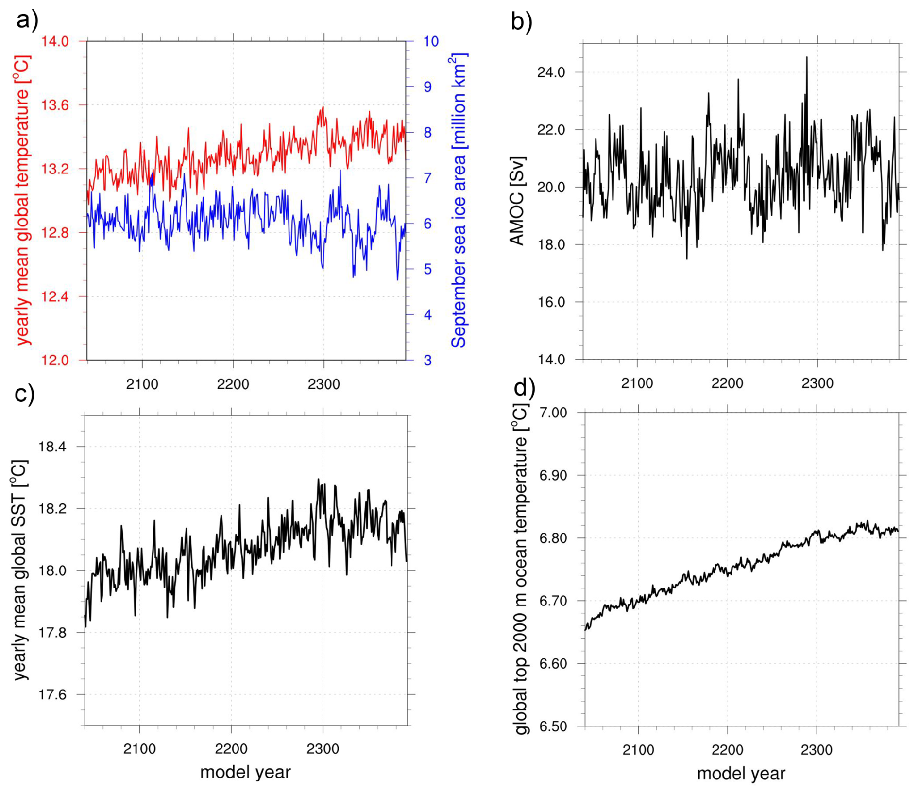
Figure A1 Time series from the 350-year EC-Earth3-HR pre-industrial (PI) control run showing: (a) annual-mean global surface air temperature (°C, red) and September sea ice area (million km², blue); (b) annual-mean AMOC strength, defined as the maximum overturning stream function between 20–40° N at 800–1100 m depth. (c) annual-mean global sea-surface temperature (SST); and (d) annual-mean global vertically averaged upper-ocean temperature (0–2000 m).

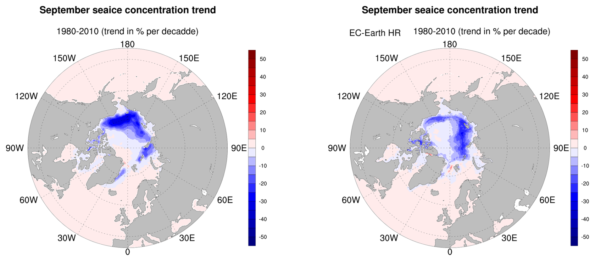
Figure A2 Trend in sea ice concentration between 1980 and 2010 (% per decade). The left panel shows satellite-observed sea ice concentration, and the right panel shows EC-Earth3-HR-simulated sea ice concentration.

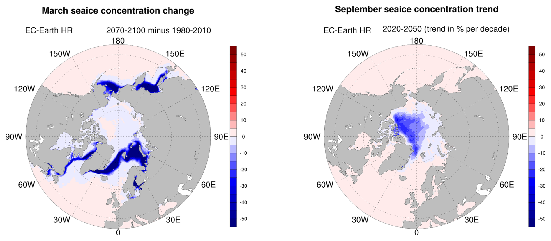
Figure A3 The left panel shows the March sea ice concentration change (%) in EC-Earth3-HR between 1980–2010 and 2071–2100 under the SSP2-4.5 scenario, and the right panel shows the September sea ice concentration trend from 2020 to 2050 (% per decade).

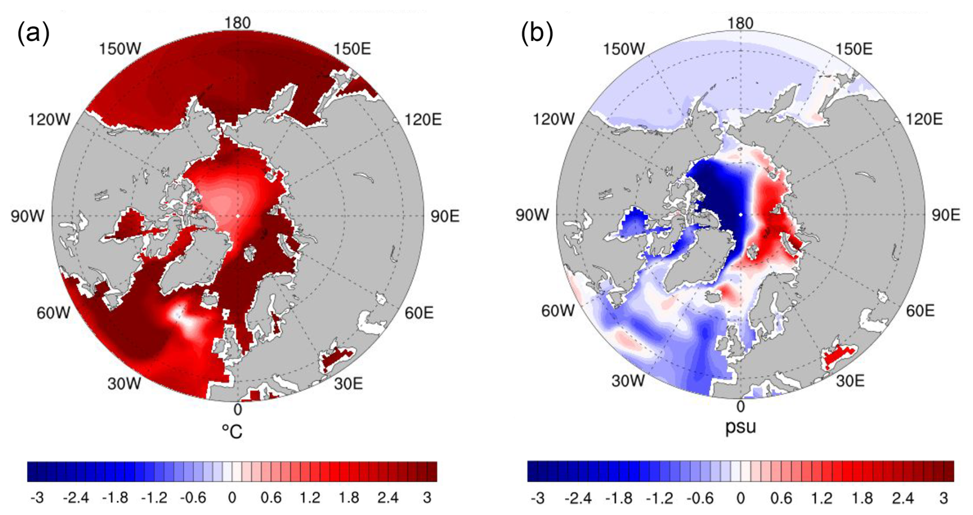
Figure A4 Differences between the 2071–2100 and 1980–2010 periods under the SSP2-4.5 scenario for the EC-Earth3-SR ensemble mean: (a) annual mean sea surface temperature (SST, °C); (b) annual mean sea surface salinity (SSS, psu).

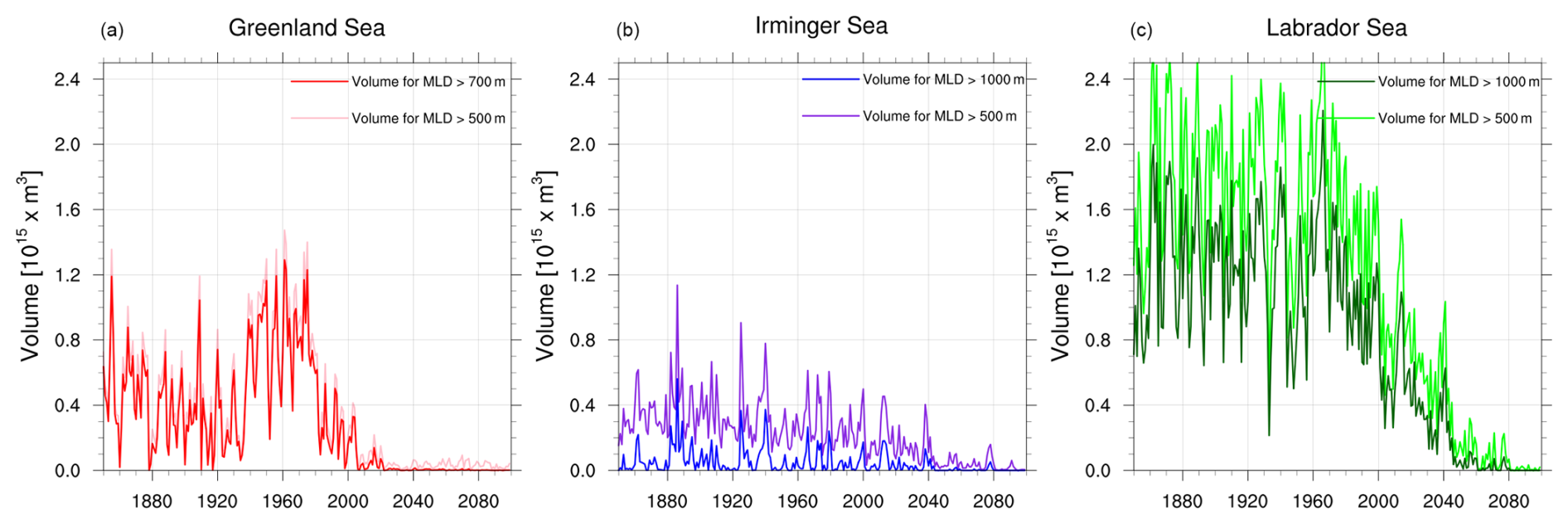
Figure A5 Deep Mixed Volume (DMV) in March for the Greenland Sea (a), Irminger Sea (b), and Labrador Sea (c) from historical and SSP2-4.5 simulations of EC-Earth3-HR. Two reference depths are shown: 700 m for the Greenland Sea and 1000 m for the Irminger and Labrador Seas (as in Fig. 10; thick lines), and 500 m for all three basins (dashed lines).

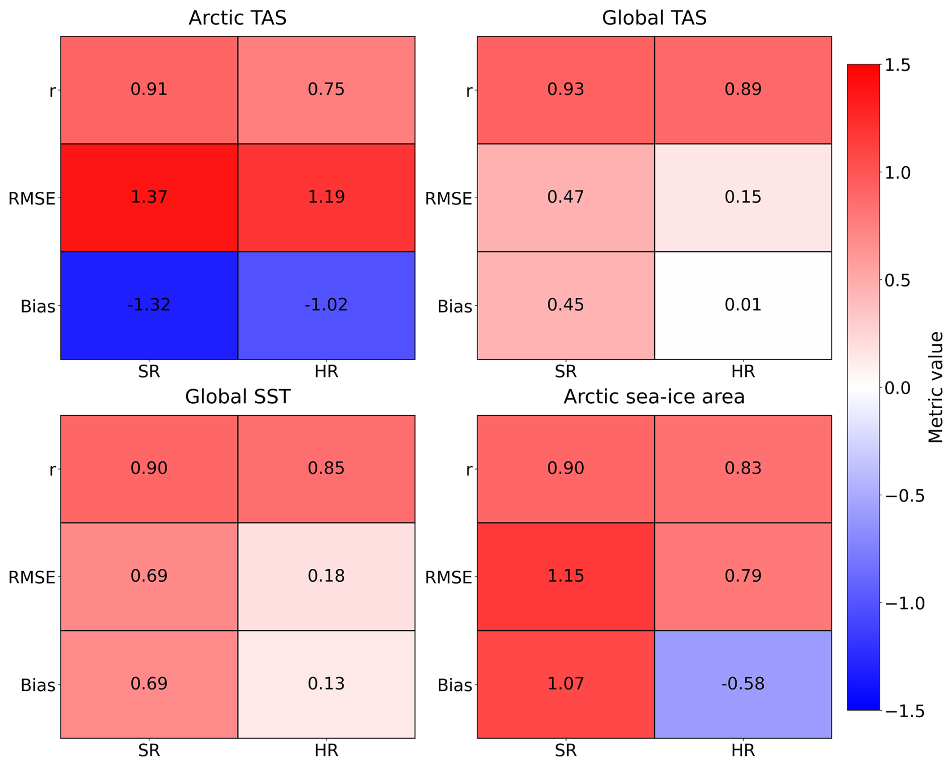
Figure A6 Quantitative evaluation of EC-Earth3-SR and EC-Earth3-HR performance relative to observations and reanalysis for Arctic and global surface air temperature (TAS), global sea surface temperature (SST), and Arctic sea-ice area. Shown are correlation (r), root-mean-square error (RMSE), and mean bias for each variable. Metrics are computed over the historical period: 1950–2014 for TAS, 1870–2014 for SST, and 1979–2014 for sea ice.

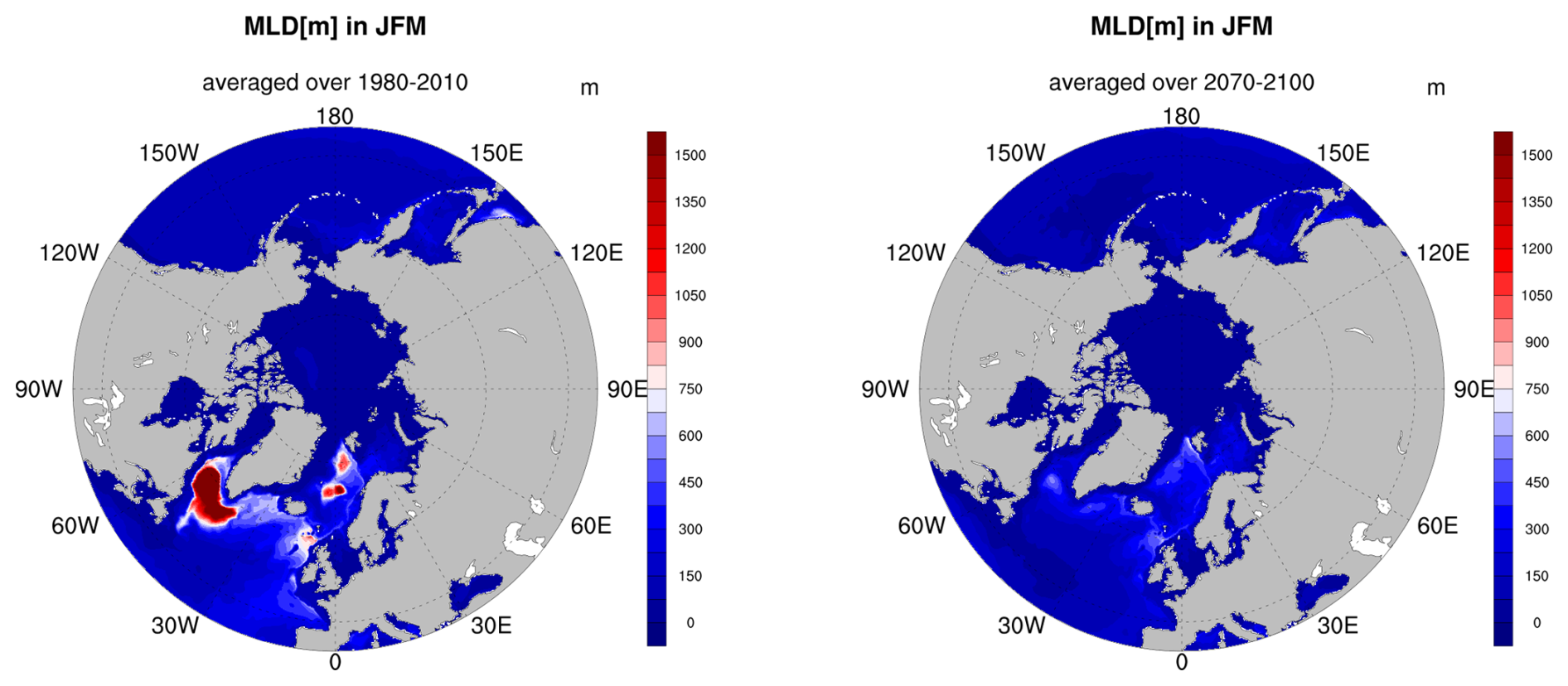
Figure A7 EC-Earth3-HR winter mean (JFM) mixed layer depth (MLD, m) averaged over 1980–2010 (left panel) and 2070–2100 (right panel).

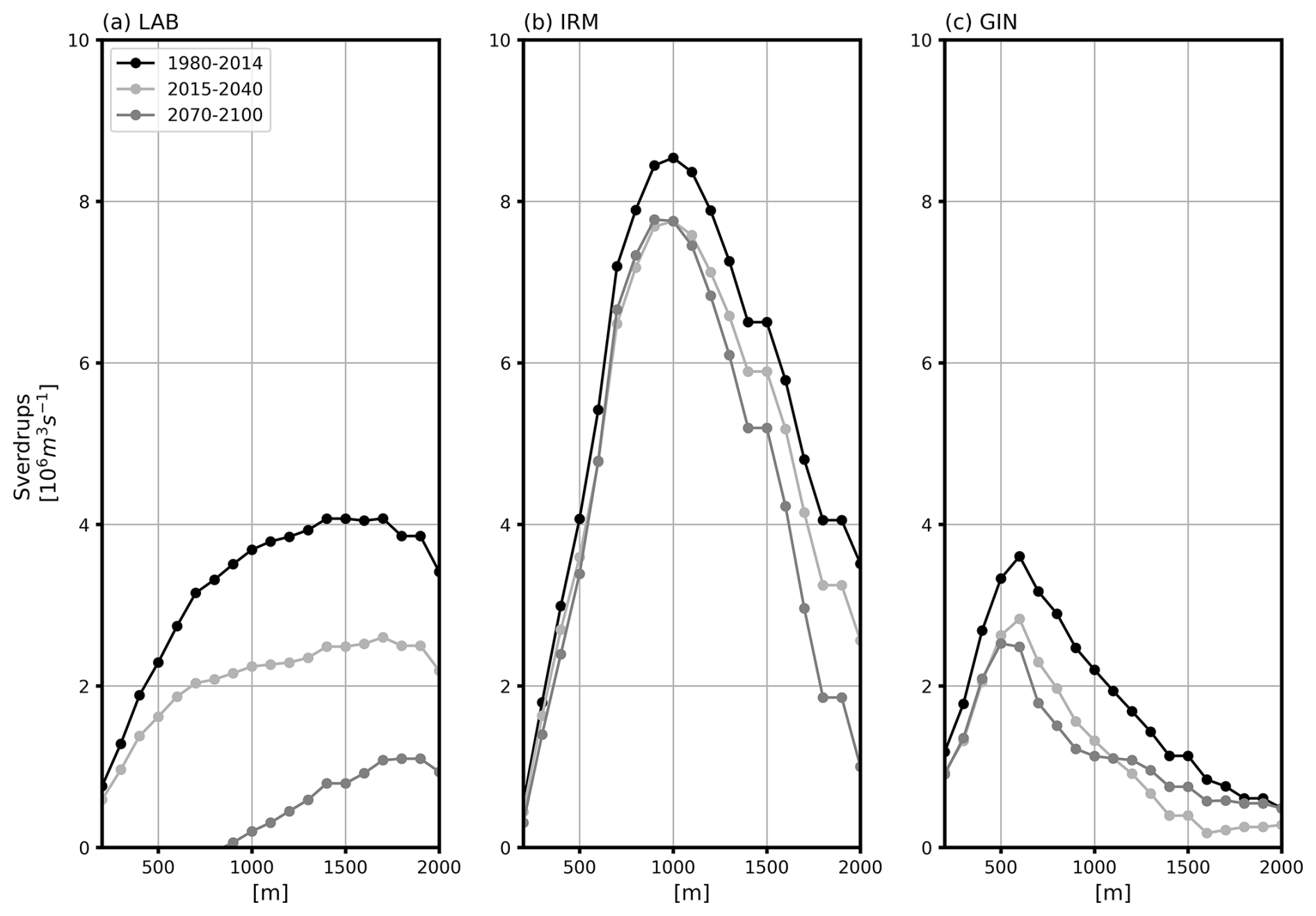
Figure A8 Sensitivity of the deep-water formation (DWF) to the choice of reference depth for the Labrador (LAB), Irminger (IRM), and GIN seas, shown for the historical period (mean over 1980–2014) and two future periods (mean over 2015–2040 and 2070–2100). While the magnitude of the DWF index depends on the reference depth, the relative regional contrasts and projected future changes are robust.