New insights into decadal climate variability in the North Atlantic revealed by data-driven dynamical models

The Atlantic Multidecadal Variability (AMV) and the North Atlantic Oscillation (NAO) are the dominant modes of oceanic and atmospheric variability in the North Atlantic, respectively, and are key sources of predictability from seasonal to decadal timescales. However, the physical processes and feedback mechanisms linking the AMV and NAO, and the role of diabatic processes in these feedbacks, remain debated. We present a data-driven dynamical modelling framework which captures coupled decadal variability in AMV, NAO, and North Atlantic precipitation. Applying equation discovery methods to observational data, we identify low-order models consisting of three coupled ordinary differential equations. These models reproduce observed decadal variability and show robust out-of-sample predictive skill on multi-annual to decadal lead times. The resulting model dynamics include a distinct quasi-periodic 20-year oscillation consistent with a damped oceanic mode of variability. Notably, precipitation-related terms feature prominently in the low-order models, suggesting an important role for latent heat release and freshwater fluxes in mediating ocean–atmosphere interactions. We propose new feedback mechanisms between North Atlantic sea surface temperature and the NAO, with precipitation acting as a dynamical bridge. Overall, these results illustrate how equation discovery can provide mechanistic hypotheses and new insight beyond conventional analyses of observations and climate model simulations.

1 Introduction

The coupled North Atlantic exhibits natural variability on a range of timescales, as well as responses to external forcings. The dominant mode of variability in the ocean, the Atlantic Multidecadal Variability (AMV), is characterised by multidecadal variations in Sea Surface Temperature (SST) anomalies (Kerr, 2000) spanning the entire North Atlantic basin. We characterise this temporal variability using an AMV index (Trenberth and Shea, 2006). The AMV has significant impacts on hemispheric and regional climates. Such impacts include altering the frequency of Atlantic hurricanes (Goldenberg et al., 2001), driving shifts in the Intertropical Convergence Zone (ITCZ) (Knight et al., 2006), forcing changes in the occurrence of droughts in the Sahel (Zhang and Delworth, 2006), and modulating European and North American summer climate (Sutton and Hodson, 2005).

The North Atlantic Oscillation (NAO) is the leading mode of atmospheric variability in the North Atlantic region. The temporal variability of the NAO is characterised by the pressure difference between the Azores (Azores high) and Iceland (Icelandic low) (Hurrell and Deser, 2010), which is defined as the NAO index. The temporal variability of the NAO exhibits a broad range of features, from interannual to multidecadal. The NAO also exerts a strong influence on the climate, especially in the Northern Hemisphere (Hurrell et al., 2003; Hurrell, 1995; Li et al., 2013). During the winter period, NAO changes are the dominant mode of European climate variability, with a positive NAO phase causing the North Atlantic storm track to orient in a more northward direction. Storm tracks in this position bring drier conditions to southern Europe and wetter conditions to northern Europe (Hurrell, 1995; Seager et al., 2020). Precipitation over the North Atlantic is also heavily influenced by the NAO (Walsh and Portis, 1999; Bojariu and Reverdin, 2002; Mariotti and Arkin, 2007).

Various mechanisms driving the decadal fluctuations in the AMV have been hypothesised, such as those arising from internal ocean variability (Bjerknes, 1964; Delworth et al., 1993; Kushnir, 1994; Trenberth and Shea, 2006) and anthropogenic aerosols and changes in Greenhouse Gases (GHG) (Bellomo et al., 2018; Robson et al., 2022; Booth et al., 2012). Other researchers provide compelling evidence that direct stochastic atmospheric forcing is also a significant driver of the AMV (O’Reilly et al., 2019; Clement et al., 2015, 2016; Cane et al., 2017), including through the integrated response to the NAO (McCarthy et al., 2015). The NAO also has predictable decadal variability (Athanasiadis et al., 2020; Smith et al., 2020) with an important role for ocean feedback (Patrizio et al., 2025). In turn, the NAO may influence the ocean through its impact on surface heat and freshwater fluxes. However, these bidirectional air–sea interactions linking the NAO and AMV on decadal and multidecadal timescales are still highly contested (Zhang et al., 2019).

Some studies point towards a direct influence of precipitation as a source of freshwater fluxes in the North Atlantic which affects the salinity and temperature of the upper ocean (Josey and Marsh, 2005; Myers et al., 2007). This is particularly important in regions of deep water formation, such as the Labrador Sea, where freshwater fluxes have direct effects on the strength and variability of the Atlantic Meridional Overturning Circulation (AMOC) (Mignot and Frankignoul, 2003; Marsh, 2000; Mehling et al., 2022). Other studies show evidence of North Atlantic precipitation feedbacks onto the NAO (Kolstad and O’Reilly, 2024; Rodwell et al., 1999) and North Atlantic storm tracks (Lau, 1988) through latent heat release. A complete picture of the bidirectional nonlinear relationships linking North Atlantic precipitation, the NAO, and AMOC/AMV has yet to be fully developed.

AI-based equation discovery is an emerging technique designed to use observations of the state of a system to discover the underlying governing equations that may have previously been unknown. This AI approach has been suggested to be useful for climate research (Huntingford et al., 2025), where it offers the potential to provide much clearer process understanding of the climate system through reduced-complexity models based on the discovered equations. In some cases, the new equations may even reveal hidden underlying physics (Brunton et al., 2016), and if the processes governing the observed data are accurately modelled, the equation representation may be capable of generalising and making predictions outside the training domain. We apply this equation discovery method to the coupled North Atlantic climate to derive a three-variable dynamical systems model from observational data. This framework links the AMV and NAO drivers to North Atlantic precipitation over decadal timescales.

Due to the significant climate impacts of the AMV, improving forecasts of the AMV state across decadal timescales would be of great socioeconomic importance, which could be facilitated by a better understanding of the AMV process through the establishment of the underlying equations. Currently, initialised decadal forecast prediction systems demonstrate substantial skill in hindcasting the AMV index (Van Oldenborgh et al., 2012; Trenary and DelSole, 2016; DelSole et al., 2013; Borchert et al., 2019) over decadal timescales. The variability of the NAO has often been considered largely as white noise, and therefore random. However, more recent ensemble forecasting has shown that its statistics are predictable on seasonal (Scaife et al., 2014), decadal (Smith et al., 2020) and projection (Smith et al., 2025) timescales. These demonstrations of skill are a result of full complexity calculations discretised over a spatial and vertical grid. For comparison, we aim to collapse this state space down to a simple three-dimensional ODE system evolving in time. If a simpler model can effectively capture the behaviours of the full model, this implies that the lower-complexity model should also possess predictive capability.

In this paper, we employ AI-based equation discovery by adopting a sparse regression procedure to derive a reduced-order model of the North Atlantic. The derived model consists of three coupled Ordinary Differential Equations (ODEs) that evolve over time. These equations link the monthly AMV and NAO indices to a precipitation index that measures the average monthly precipitation anomalies in the North Atlantic region. The aim is to use the identified equation set to uncover the slow-evolving dynamics arising from ocean variability and ocean-atmosphere interactions, along with feedbacks involving precipitation. Utilising the equation discovery approach opens the door to new process understanding of the coupled North Atlantic climate.

In Sect. 2.2 we describe how we learn dynamical systems equations from ERA5 reanalysis data using the Sparse Identification of Nonlinear Dynamics algorithm (Brunton et al., 2016). The candidate models are presented in Sect. 3.1 and the predictive capabilities of such models are demonstrated in Sect. 3.2.1. In Sect. 3.3, we use the dynamical models to isolate and understand the associated mechanisms of decadal variability as seen in observations. From this, we provide a new understanding of ocean-atmosphere feedback in the North Atlantic by highlighting the active role precipitation plays in these interactions.

2 Data and Methods

2.1 Data

ERA5 and ERA20C

We learn dynamical system models using the European Centre for Medium-Range Weather Forecasts (ECMWF) Reanalysis 5 (ERA5) dataset (Hersbach et al., 2020) spanning the period from January 1950 to December 2022, which we treat as our observational “truth”. We use this data at a temporal resolution of one month, and on a spatial grid of 0.5° × 0.5°. To assess how well the family of potential discovered equations predicts data it has not been compared against, we construct an additional validation and test set.

Selecting a model based on the validation set rather than the training data avoids the possibility of choosing a model that has overfitted to the training data. The test data is then used to assess the ability of the best model to predict unseen data. For testing and validation, we use different segments of the ECMWF Reanalysis of the 20th Century (ERA20C) dataset (Poli et al., 2016) over the period from January 1900 to December 1949. Specifically, we make data from January 1940 to December 1949 to be our validation set, and from January 1900 to December 1939 as our test set.

Precipitation in the ERA5 reanalysis data is not an assimilated variable before 2010, up to which point it is only a modelled field. The Global Precipitation Climatology Project (GPCP) Monthly Analysis Product (Adler et al., 2003) spans 1979 to the present and integrates data from rain gauge stations and various satellite datasets over land and ocean. Thus, for 1979 onward, the GPCP dataset provides one of the most complete and accurate rainfall analyses over the oceans. The correlation between GPCP and ERA5 monthly precipitation anomalies over the North Atlantic ocean (see Sect. 2.2 for area of interest) is 0.4 for the period 1982–2020. However, unlike GPCP, ERA5 provides a consistent dataset between 1950 and the present, which is sufficiently long to learn low-order models that capture decadal variability.

We favour the later ERA5 dataset for model training, as improved data assimilation techniques and the abundance of satellite and ground observations result in a more accurate and trustworthy representation of historical Atlantic variability than in the ERA20C data (Hersbach et al., 2020; Poli et al., 2016). This additional accuracy is likely especially valid regarding precipitation over the Atlantic Ocean. The ERA20C dataset is longer than ERA5 but only assimilates surface observations. We choose our validation set to be a relatively short 20 % of the independent period (1900 to 1949), as we favour longer periods to evaluate the ability of a low-order model to predict the decadal variability of the AMV, NAO, and precipitation indices for various different states of the system. The correlation coefficient between monthly North Atlantic precipitation anomalies (see Sect. 2.2 for area of interest) derived from ERA5 and ERA20C datasets is strong at 0.89 for the shared period 1950–2010.

2.2 Methods

2.2.1 Metrics

To compute the AMV index, the mean monthly SST anomalies are calculated for the region (80–0° W, 0–60° N), from which we subtract the global average (60° S–60° N) following Trenberth and Shea (2006). We then normalise the index by dividing by its standard deviation. The NAO index is defined as the difference between the mean monthly sea level pressure anomalies for a region around the Azores (28–20° W, 36–40° N) and around Iceland (25–16° W, 63–70° N) following Dunstone et al. (2016). The NAO time series is then normalised by dividing by its standard deviation. We compute North Atlantic precipitation time series as the mean monthly total precipitation anomalies for the region (60–0° W, 15–75° N). We denote these anomalies with P, which have units of m. The precipitation index is then normalised by dividing by its standard deviation, as performed for the NAO and AMV indices. All three indices, AMV, NAO and P have zero mean across the period 1950–2022, as they were computed using monthly anomalies of SST, sea-level pressure, and total precipitation based on the climatology of the full period. Since all time series have been normalised, they are therefore all unitless.

2.2.2 Sparse Identification of Nonlinear Dynamics (SINDy)

Sparse Identification of Nonlinear Dynamics (SINDy) (Brunton et al., 2016) is a sparse regression algorithm that learns dynamical system equations from data time series, and here in the form of ordinary differential equations. A general time-evolving dynamical systems model takes the form of $\dot{\mathit{x}}\left(t\right)=\mathit{f}\left(\mathit{x}\right(t\left)\right)$ where the vector $\mathit{x}=\begin{array}{cccc}\left[x_{\mathrm{1}}\right(t)& x_{\mathrm{2}}\left(t\right)& \cdot \cdot \cdot & x_d\left(t\right){]}^{\mathrm{T}}\in {\mathbb{R}}^d\end{array}$ represents the state of the system at time, t. The number of system variables is represented by d and we have m observations of the state x. The SINDy algorithm learns the analytical form of f from data, by performing a regression analysis using a library of candidate functions. SINDy assumes the function, f, is sparse, and therefore operates to deliberately contain only a few terms from these candidate functions.

We use the SINDy algorithm to fit dynamical models evolving in time to the AMV index (AMV), NAO index (NAO) and North Atlantic precipitation anomalies (P). Since we are interested in the relationships between state variables on longer decadal timescales, a twelve-month running average is applied to the three variable time series spanning the training set from January 1950 to December 2022, after which the model is fitted. This approach removes higher frequency signals and improves the performance of fitting, consequently enhancing the quality and stability of the resulting dynamical models. Our chosen library of candidate functions consists of an offset term and linear and nonlinear polynomial terms of the three state variables up to order two. This gives a total of ten terms in each of the three equations for each state variable, resulting in 30 terms overall, describing the time evolution of the system variables. Given that the data set is limited in length, we choose polynomial terms only up to order two to reduce the risk of overfitting. The general form for the model with our candidate functions is:

$$\begin{array}{}\text{(1)}& {\displaystyle \frac{\mathrm{d}{x}_i}{\mathrm{d}t}}=a_i+\sum _{j=\mathrm{1}}^{\mathrm{3}}{b}_{ij}{x}_j+\sum _{\mathrm{1}\le j\le k\le \mathrm{3}}{c}_{ijk}{x}_j{x}_k,i=\mathrm{1},\mathrm{2},\mathrm{3},\end{array}$$

where x₁, x₂ and x₃ are the state variables AMV, NAO and P respectively. In Eq. (1), a constant term in each equation is represented by a_i, the coefficients of the linear terms are represented by b_ij, and the coefficients of unique quadratic cross-products and squares are represented by c_ijk. The 30 coefficients are solved for simultaneously in the equation discovery process. To solve for these coefficients, we require observations of the instantaneous changes, $\frac{\mathrm{d}{x}_i}{\mathrm{d}t}$. These are computed numerically from the data. The candidate functions are evaluated at every point in time using observations of the state variables. The SINDy algorithm then regresses $\frac{\mathrm{d}{x}_i}{\mathrm{d}t}$ against the observed values of the candidate functions to find the unknown coefficients a_i, b_ij, and c_ijk.

To perform the regression, we use the LASSO optimiser, which introduces sparsity into the regression procedure. It does this by adding a penalty to the sum of the absolute values of the regression coefficients, resulting in some coefficients becoming exactly zero, thereby excluding less important variables and preventing overfitting – this is called “regularisation” in the ML community. The threshold parameter, λ, determines the strength of the penalty: coefficients are set to zero if their magnitude is less than λ.

We use two approaches to improve the robustness of the fitted model. Firstly, we use an “ensembling” approach. We randomly sample the data with replacement to create 1000 “bootstrapped” datasets before fitting a model to each one. We then take the median coefficients across the ensemble of 1000 models to produce a final averaged model. The sizes of the random samples are taken to be 25 %, 50 %, 75 % of the total number of data points in the data matrix X. Since we have three monthly time series then d=3, and these span January 1950 to December 2022 inclusive, meaning m=876. Therefore, we have a total of $d\times m=\mathrm{2628}$ data points. We also fit models using 100 % of the training data without bootstrapping.

Secondly, we apply “sparsity thresholding” in the learning process. This repeats the ensembling process for a range of threshold values, λ. Here we choose lambda to range from 0 to 1 with a step of 0.005. By using the four different bootstrap sample sizes and 200 different possible values of lambda, we learn a total of 800 candidate models when both ensembling and sparsity thresholding are applied. We finally discard any duplicate models, such as those which contain no terms due to the sparsity threshold being too high, or those with the exact same coefficients. The remaining set of candidate models is then evaluated on the validation data set.

2.2.3 Statistical significance

The statistical significance of the low-order model's predictive performance in Sect. 3.2.1 (quantified using anomaly correlation coefficients) accounts for autocorrelation by performing block bootstrapping on model forecasts and observations, followed by a one-sided Student's t test against the null hypothesis of non-positive (negative) correlation, applied at the 0.05 significance level. We use a one-sided Student's t test as we are only concerned with the “positive skill” of the low-order model, since negative correlations are evidence of “anti-skill”. When computing regressions between indices and other variables in Sect. 3.3, significance levels are computed based on a random phase test (Ebisuzaki, 1997). Here, we generate 10 000 phase-randomised surrogates of the index that preserve its power spectrum (and autocorrelation), and compute the regression coefficients between the surrogate distribution and the chosen variable time series. The null hypothesis is that a correlation arises purely from internal serial correlation. We apply this test at the 95 % significance level.

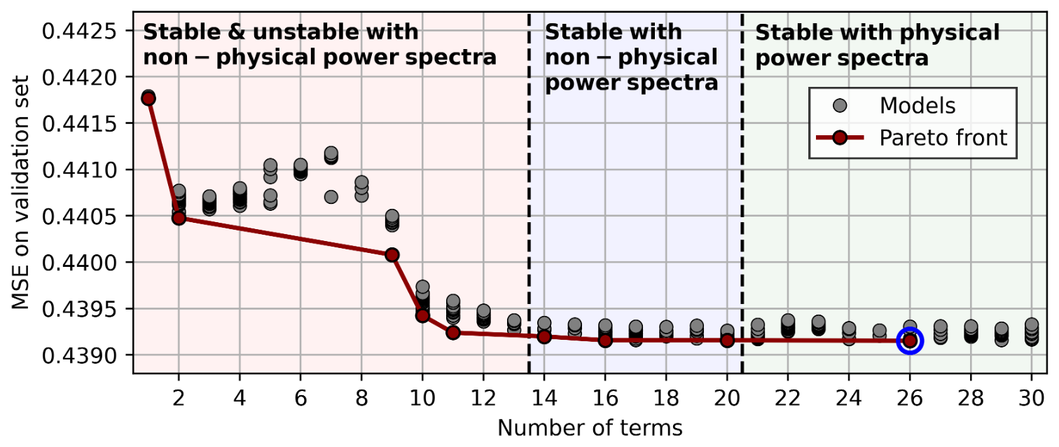
Figure 1 Model selection. Mean Squared Error (MSE) of the instantaneous tendencies from the low-order models as a function of the number of retained terms in the equations (grey circles), as assessed using the validation dataset. The Pareto front is shown as a red curve, indicating the models that maximise predictive accuracy and for each level of complexity. Models with up to thirteen terms have either unstable or stable behaviours, with all models having non-physical power spectra (red region). Models containing between 14 and 20 terms are stable but also produce non-physical power spectra (blue region). Potential models with the number of terms greater than, or equal to, 21 are stable and have physically realistic power spectra (green region). The blue circle indicates the model on the Pareto front with 26 terms, which we choose as our “best” model.

3 Results and Discussion

3.1 The low-order dynamical models

Employing the method of sparse identification of nonlinear dynamics on the three time series of the AMV index, NAO index and North Atlantic precipitation anomalies, as retrieved from the ERA5 reanalysis dataset, yields a set of candidate models based on the ensembling and thresholding procedures outlined in Sect. 2.2. These models are in the form of three coupled first-order ordinary differential equations, with the algebraic components consisting of nonlinear polynomial terms up to second order. These polynomial terms may contain cross-terms; that is, the composition of a second-order term may be a mixture of the three state variables. Following the procedure as outlined in Sect. 2.2, we obtain a total of 344 unique candidate models, with varying degrees of sparsity. The mean squared error (MSE) between the instantaneous predicted derivatives and the derivatives of the observed variable time series from the ERA5 validation set is computed for each model. This MSE, as a function of the number of non-zero terms in the models, is represented by the grey dots shown in Fig. 1. In general, there are several candidate models for each given number of terms. As the equations become more complex, corresponding to more equation terms, we see a general decrease in model error (Fig. 1). However, too many equation terms and excessive complexity could introduce “over-fitting”, leading to spurious effects in the models. A Pareto front is constructed, which determines the best compromise between maximising accuracy while simultaneously reducing complexity. This front is shown as the red curve in Fig. 1. A model is “Pareto optimal” if you cannot improve one objective without making another worse, these models are indicated by the red markers. As a test of sensitivity, we note that the Pareto front does not substantially change when we assign different sections of unseen data (January 1900 to December 1949) as our validation set.

3.1.1 Three candidate models

We consider three sets of potential equations, each with a different number of terms, selected based on the Pareto curve in Fig. 1. The Pareto curve illustrates how errors begin to plateau for models with ten or more terms, indicated by the “knee” point of the Pareto front (Fig. 1). Thus, we could choose a ten-parameter model as our “best” model, as it achieves a good trade-off between model accuracy and complexity. The ten-term model with the lowest MSE is given by Eqs. (2)–(4):

$$\begin{array}{}\text{(2)}& {\displaystyle }\begin{array}{lclcl}\mathit{\tau }\frac{\mathrm{d}A}{\mathrm{d}t}=& & -\mathrm{1.61}N& & \\ & & & & -\mathrm{1.63}NP\end{array}\text{(3)}& {\displaystyle }\begin{array}{llcll}\mathit{\tau }\frac{\mathrm{d}N}{\mathrm{d}t}=& +\mathrm{1.21}A& & & -\mathrm{0.66}{A}^{\mathrm{2}}\\ & & & +\mathrm{2.39}AP& +\mathrm{1.58}NP\end{array}\text{(4)}& {\displaystyle }\begin{array}{lccll}\mathit{\tau }\frac{\mathrm{d}P}{\mathrm{d}t}=& & & & +\mathrm{0.95}{A}^{\mathrm{2}}\\ -\mathrm{0.62}{N}^{\mathrm{2}}& & & -\mathrm{1.37}AP& -\mathrm{1.41}NP\end{array}\end{array}$$

where “A” refers to the AMV index, “N” refers to the NAO index, and “P” refers to the precipitation anomalies of the North Atlantic. This model falls on the Pareto front, and is marked by a red dot in Fig. 1. The natural time step, t, is months, as this corresponds to the time interval of the data. However, as we expect the SINDy methodology to quantify the longer-term variations, we have scaled the equations by multiplying through by τ=120 months (10 years). Hence, each coefficient represents the decadal tendencies of each term. Notably, this scaling makes all terms on the right-hand side of Eqs. (2)–(4) of order unity thus balanced in magnitude, illustrating that this timescale is the one for which the SINDy algorithm is identifying changes.

To assess the model's validity, we must also examine its long-term behaviour. Due to the limited period for which data on A, N, and P are available, long-term behaviour does not form part of the SINDy fitting process, which can only be expected to capture variations up to timescales of the order of decades. However, the current observations clearly illustrate that the coupled A–N–P system exhibits substantial variability, and arguably this allows us to eliminate equation sets that fail to account for this behaviour over the longer term. Hence, we numerically integrate Eqs. (2)–(4) forward, using a fourth-order Runge-Kutta scheme, and find that all solutions of this model converge onto one of the five stable fixed points: ($A=-\mathrm{1.20}$, N=0, $P=-\mathrm{0.84}$), (A=0, N=0, $P=-\mathrm{0.99}$), ($A=-\mathrm{3.29}$, $N=-\mathrm{2.15}$, $P=-\mathrm{0.99}$), ($A=-\mathrm{1.04}$, N=0.31, $P=-\mathrm{0.99})$ and (A=0.83, $N=-\mathrm{0.91}$, $P=-\mathrm{0.99}$). Once the solutions of this model converge onto stable fixed points, they remain at a constant value for all time. Hence, this equation set does not represent self-sustaining variability in the North Atlantic and therefore is an unrealistic model. More generally, we find that all models with thirteen terms or less (red region in Fig. 1) either converge on stable fixed points, limit cycles, or are unstable and lead to “blow-ups” in the simulated trajectories. A limit cycle is an isolated closed trajectory in phase space that represents a stable, self-sustained oscillation. Models that follow limit cycles may generate observed variations in A, N and P, however, they may also lack important features of the observed variability.

For this reason, in addition to requiring that our model has a low MSE concerning instantaneous tendencies, we also introduce a second requirement that a credible model has realistic variability on longer timescales. This comparison is based on the estimated power spectra derived from model integrations undertaken for 50 000 years. Considering models with more terms in the equations, we find that those which contain between fourteen and twenty terms, inclusive, are all stable when integrated forward in time and have solutions that either converge onto a limit cycle or a stable fixed point (blue region in Fig. 1). One such model is the 16-term Pareto-optimal model, shown below (Eqs. 5–7), whose solutions converge onto a limit cycle:

$$\begin{array}{}\text{(5)}& {\displaystyle }\begin{array}{lllll}\mathit{\tau }\frac{\mathrm{d}A}{\mathrm{d}t}=& & -\mathrm{1.69}N& & +\mathrm{0.52}{A}^{\mathrm{2}}\\ & +\mathrm{0.59}{P}^{\mathrm{2}}& & -\mathrm{1.53}AP& -\mathrm{1.93}NP\end{array}\text{(6)}& {\displaystyle }\begin{array}{lllll}\mathit{\tau }\frac{\mathrm{d}N}{\mathrm{d}t}=-\mathrm{0.90}& +\mathrm{1.33}A& & & -\mathrm{0.65}{A}^{\mathrm{2}}\\ & +\mathrm{0.71}{P}^{\mathrm{2}}& -\mathrm{0.81}AN& +\mathrm{1.94}AP& +\mathrm{1.64}NP\end{array}\text{(7)}& {\displaystyle }\begin{array}{lccll}\mathit{\tau }\frac{\mathrm{d}P}{\mathrm{d}t}=& & & & +\mathrm{0.82}{A}^{\mathrm{2}}\\ -\mathrm{0.74}{N}^{\mathrm{2}}& & & -\mathrm{1.35}AP& -\mathrm{1.43}NP\end{array}\end{array}$$

and where the notation and variable names are identical to those of Eqs. (2)–(4). While this model is stable and converges on a limit cycle representing long-term oscillations in the North Atlantic, its behaviour is not realistic when compared to the observed North Atlantic. Upon inspection of the simulated power spectra of the candidate model ensemble, we see that models which contain 20 or fewer terms are unable to produce the broad-band physical power spectra seen in observations. These models have sparse spectra, with delta-like peaks at particular frequency bins, associated with the limit cycle. The limit cycle of Eqs. (5)–(7) is shown in the three-dimensional phase space plots in Fig. 2a–c. While this captures the interconnected behaviour of the NAO, AMV, and precipitation in this region, it does not capture the irregular nature of the dynamics of the North Atlantic.

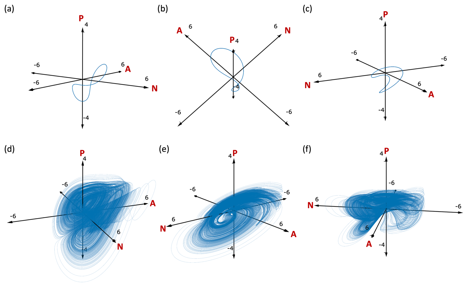
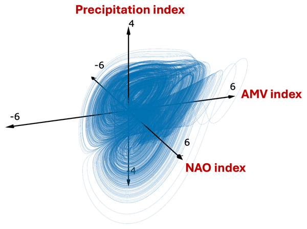
Figure 2 Model attractors. Phase space plots displaying model attractors obtained by initializing the model and simulating for 50 000 years with a 1 month time step. Panels (a)–(c) show the limit cycle produced by the 16-term model given by Eqs. (5)–(7). Panels (d)–(f) show the chaotic attractor of the 26-term model given by Eqs. (8)–(10). The axes are unit-less as the variables were normalised prior to model training.

Upon further increasing the number of terms, we find that all models with 21 terms or more exhibit long-term stability and have solutions with broad-band power spectra (green region in Fig. 1); these models possess chaotic attractors. The final point on the Pareto front (blue circle in Fig. 1) identifies a model containing 26 terms, which generates physically consistent broad-band power spectra when compared to observations. For the remainder of this paper, we choose this model as our “best” candidate model for further exploration, and we refer to it as the “low-order model”. The analytical form of the low-order model is shown in Eqs. (8)–(10):

$$\begin{array}{}\text{(8)}& {\displaystyle }\begin{array}{lllll}\mathit{\tau }\frac{\mathrm{d}A}{\mathrm{d}t}=-\mathrm{0.29}& -\mathrm{0.18}A& -\mathrm{1.75}N& & +\mathrm{0.67}{A}^{\mathrm{2}}\\ -\mathrm{0.11}{N}^{\mathrm{2}}& +\mathrm{0.67}{P}^{\mathrm{2}}& +\mathrm{0.51}AN& -\mathrm{1.72}AP& -\mathrm{2.07}NP\end{array}\text{(9)}& {\displaystyle }\begin{array}{lllll}\mathit{\tau }\frac{\mathrm{d}N}{\mathrm{d}t}=-\mathrm{1.05}& +\mathrm{1.45}A& +\mathrm{0.57}N& -\mathrm{0.53}P& -\mathrm{0.63}{A}^{\mathrm{2}}\\ & +\mathrm{0.66}{P}^{\mathrm{2}}& -\mathrm{0.91}AN& +\mathrm{2.08}AP& +\mathrm{1.74}NP\end{array}\text{(10)}& {\displaystyle }\begin{array}{lllll}\mathit{\tau }\frac{\mathrm{d}P}{\mathrm{d}t}=+\mathrm{0.51}& & -\mathrm{0.68}N& & +\mathrm{0.85}{A}^{\mathrm{2}}\\ -\mathrm{0.72}{N}^{\mathrm{2}}& +\mathrm{0.12}{P}^{\mathrm{2}}& +\mathrm{0.34}AN& -\mathrm{1.44}AP& -\mathrm{1.38}NP\end{array}\end{array}$$

This set of three ODEs (Eqs. 8–10) exhibit a very broad range of behaviours, including elements of both transient chaos and strong predictability. The model attractor in phase space is shown in Fig. 2d–f, obtained by simulating a 50 000-year trajectory from a randomly generated initial condition with a time step of 1 month. In panels (d) and (e) we observe two “sides” of the attractor, where in (d) the trajectories diverge on the left-hand side onto one of the two wings of the attractor, similar to the Lorenz (1963) model. In panel (e), we observe that points travelling around the wings are funnelled in towards the centre of the attractor. This phenomenon can also be observed in the top-left-hand side of panel (f).

Upon examining the analytical forms of the 10-term model (Eqs. 2–4), 16-term model (Eqs. 5–7) and the 26-term model (Eqs. 8–10) we see common terms appearing in all three models. For instance, some of the largest polynomial terms governing the dynamics of the AMV (Eqs. 2, 5, 8) include a negative linear NAO term, and for the NAO (Eqs. 3, 6, 9), a positive linear AMV term. The coefficients of these terms across the three models vary slightly in magnitude but consistently maintain positive or negative signs. This contrasts with findings in past literature. For example, O’Reilly et al. (2019) demonstrated that low-frequency AMV variability is proportional to the low-pass filtered NAO index, where a positive increase in the NAO leads to positive changes in the AMV. This finding has been used by Sun et al. (2015), to construct a delayed oscillator model for the quasi-periodic multidecadal variability of the NAO. However, in our equations governing the AMV (Eqs. 2, 5, 8), we find that positive linear NAO values cause a decrease in the AMV due to the negative coefficient. This observation aligns more closely with heat-flux forcing of the NAO on SSTs in the subpolar North Atlantic (Khatri et al., 2022, 2024). In this case, positive NAO forcing causes positive zonal wind stress anomalies, which enhances southward Ekman transport in the SPNA, leading to immediate cooling in the ocean surface (Eden and Willebrand, 2001). It is plausible that the model is extracting decadal SPNA SST signals from the AMV index, since Wills et al. (2019) demonstrated that the traditional AMV index is an average of several different processes occurring on different timescales. Upon removing shorter time-scale processes by decadal smoothing of the AMV index, the SST signal is indeed confined to the subpolar North Atlantic (SPNA) (Strommen et al., 2023). This will be explored further in Sect. 3.3.

Other terms with the largest coefficients across the three models (Eqs. 2–10) are cross terms between precipitation and the modes of variability (AP and NP). These cross terms dominate the equations for all three state variables.

For the AMV and precipitation equations, these terms have negative coefficients, while for the NAO equations, they have positive coefficients. The significance of these terms across the three models highlights the important role precipitation plays in the dynamics of large-scale variability. As precipitation is a good proxy for latent heating (Zhao et al., 2024; Kolstad and O’Reilly, 2024), these cross terms can capture highly nonlinear diabatic processes that act as a bridge between the ocean and the atmospheric circulation (Kolstad and O’Reilly, 2024). It is also possible that precipitation influences the AMV directly through freshwater fluxes (Josey and Marsh, 2005; Marsh, 2000), which then feeds back onto the atmospheric circulation. A proposed mechanism linking the AMV and NAO with precipitation will be outlined in Sect. 3.3.

Further nonlinear quadratic dynamical dependencies of the AMV and NAO were uncovered by Vannitsem et al. (2025) when they considered their low-frequency variability (greater than one year). They found a significant negative dependence of the quadratic AMV variability on the NAO, which is consistent with the three low-order dynamical models in Eqs. (3), (6), (9). In Vannitsem et al. (2025), they also found a quadratic self-dependence of the AMV (present in Eqs. 5, 8) and a strong influence of a quadratic NAO on the AMV (only found in the 26-term model in Eq. 8).

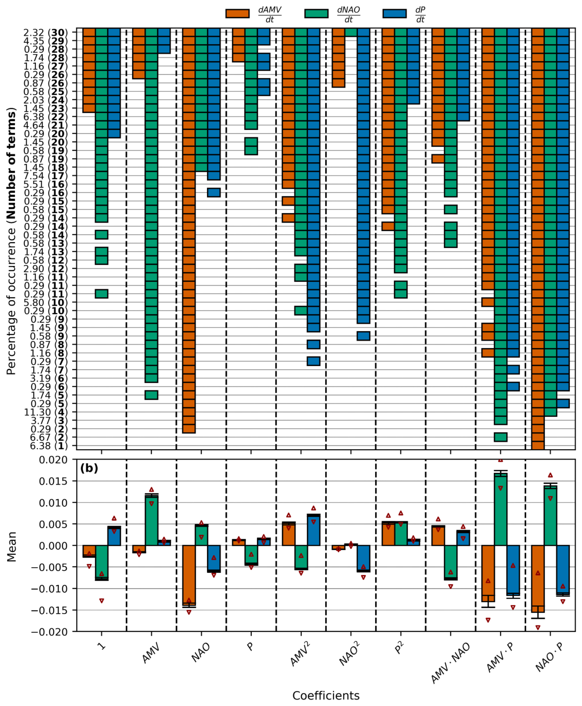
Figure 3 Model terms. (a) The polynomial terms across the entire set of 344 candidate models, based on bootstrapping. The y axis shows the total number of terms in each model (in bold font) and the occurrence of that specific model class as a percentage of the total number of models (in normal font). The x axis indicates which term in the equation is being considered for the rate of change of the AMV index (orange bars), the NAO index (green bars), and the precipitation index (blue bars) respectively. Terms that appear more often are robustly detected in the data across many different fitted models and are therefore more likely to be physical. (b) Statistics of the coefficients for each polynomial term across the entire model set. The coloured bars indicate the mean coefficient value for each retained term describing the rate of change of the AMV index (orange bars), the NAO index (green bars), and the precipitation index (blue bars). The black error bars show the interquartile range, and the red triangles indicate the minimum and maximum coefficient values.

3.1.2 The whole model ensemble

In Sect. 3.1.1, we explored the structure and terms in three models generated by the SINDy algorithm. However, our approach generates a total of 344 candidate models using the procedures outlined in Sect. 2.2. These models exhibit varying degrees of sparsity, from 1-term to the full 30-term models, as shown in Fig. 1. Examining this ensemble as a whole provides further insights into the robustness of each term in the three models, which, in turn, provides information on the dominant interactions between variables. This analysis helps to distinguish terms related to noise from those representing true dynamics in the more complex low-order models. We now present the complete set of 344 candidate models in Fig. 3. In panel (a), we show the presence of polynomial terms across the entire set of models. The x axis indicates which term in the equation is being considered for each of the $\frac{\mathrm{dAMV}}{\mathrm{d}t}$ (orange), $\frac{\mathrm{dNAO}}{\mathrm{d}t}$ (green), and $\frac{\mathrm{d}P}{\mathrm{d}t}$ (blue) equations, respectively. The y axis displays the total number of terms in each model, ranging from 1 to 30 (shown in bold), along with the occurrence of that specific model class as a percentage of the total number of models (in normal font). For each equation in each model, a filled rectangle in the figure indicates the presence of that term.

In panel (b), we present the statistics of the coefficients for each polynomial term across the entire set of candidate models. The coloured bar indicates the mean value, error bars show the interquartile range, while the red triangles indicate the minimum and maximum values for each coefficient. Since the models were trained using standardised indices (they are dimensionless), the coefficients do not relate to the units of the variables but instead indicate the importance of each term. Since models have been fitted on four bootstrapped subsets of the data (see Sect. 2.2), and while simultaneously varying the threshold parameter, λ, many models with the same number of terms can exist but differ based on small deviations in their coefficients. In some cases, two models with the same number of terms can differ based on their polynomial structure, such as the three 11-term model classes in panel (a), which also contain multiple models in each class due to differences in coefficients.

As with the 10-term, 16-term, and 26-term models described earlier in Eqs. (2)–(10), the same dominant terms across the full spectrum of fitted models are evident in Fig. 3a. As we move down the y axis in (a), we observe decreases in the number of equation terms, but the cross terms AP and NP persist for even the most sparse models, as seen in the final two triplets of columns in Fig. 3. The fact that these cross terms are robustly detected across many models for all three equations, $\frac{\mathrm{dAMV}}{\mathrm{d}t}$ (orange), $\frac{\mathrm{dNAO}}{\mathrm{d}t}$ (green), and $\frac{\mathrm{d}P}{\mathrm{d}t}$ (blue), suggests that these terms are more likely to be physical. The persistence of cross-terms involving precipitation across all models suggests that precipitation holds important dynamical information for AMV-NAO coupling. Moreover, it may act as a state-dependent coupling parameter, modifying the effective strength and sign of interactions between the AMV and NAO. Additionally, there is a delayed appearance of the $\frac{\mathrm{d}P}{\mathrm{d}t}$ equations, which occurs when models have five terms or more. In the most sparse models, precipitation serves as a diagnostic variable, where its current state provides useful information about the coupled ocean-atmosphere system. However, its own evolution may be too noisy or weak to resolve compared to the leading-order AMV-NAO interactions. Only when the model includes sufficient coupling terms can precipitation become dynamically active, allowing the lower-frequency deterministic component of precipitation to be separated from the unresolved noise. The emergence of the $\frac{\mathrm{d}P}{\mathrm{d}t}$ equations suggests an important role for active precipitation feedbacks on the atmosphere–ocean system, involving latent heating, freshwater fluxes, and atmospheric stability. We note that other robust terms are also present, such as the linear AMV term in the NAO equations and the linear NAO term in the AMV equations. A key takeaway from this section is that the robust terms across the low-order model ensemble highlight precipitation as an important mediator between the ocean and atmosphere in the North Atlantic. This coupling will be explored further in Sect. 3.3.

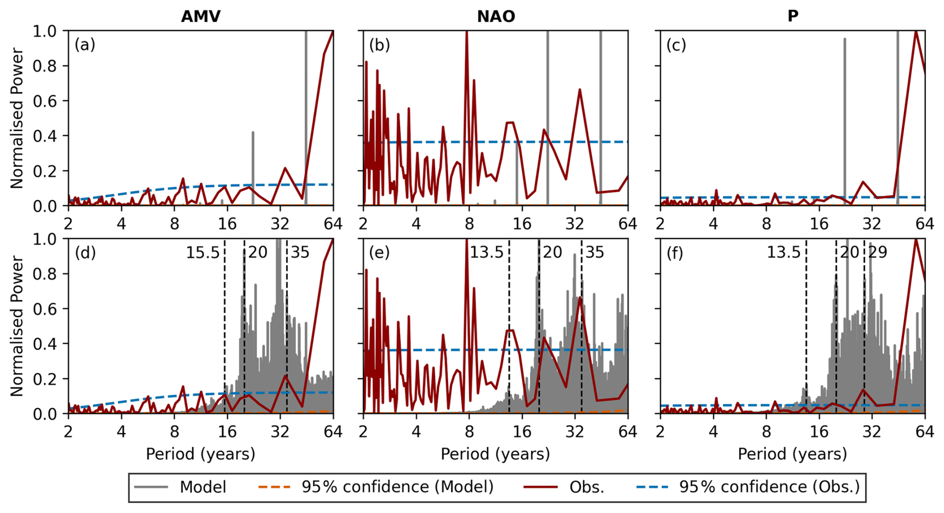
Figure 4 Model power spectra. Power spectra of 50 000 year-long model simulations (grey lines) for the 16-term model (top row a–c) and the “best” 26-term model (bottom row d–f). Power spectra for AMV are shown in the first column (a, d), NAO in the second column (b, e), and precipitation in the third column (c, f). Red line shows the power spectra of monthly observations spanning January 1900 to December 2022. Vertical black lines (d–f) indicate the positions of dominant peaks in the model power spectra. Dashed lines represent confidence intervals for accepting a red noise null hypothesis.

3.2 The chosen low-order model

From this point, we choose to focus on the 26-term model in Eqs. (8)–(10), which we will refer to as the “low-order model”. We selected this based on its ability to produce physical broad-band power spectra and its good fit to validation data (see Fig. 1). Generating power spectra from the simulated variables of the low-order model allows for the assessment of the timescales of variability extracted from observational data (Fig. 4). The model is integrated forward in time for 50 000 years, after which we compute the power spectra of (d) the AMV index, (e) the NAO index, and (f) the precipitation index. For comparison, we construct the power spectra of the observed monthly time series from January 1900 to December 2022 using a combination of ERA20C from January 1900 to December 1949 and ERA5 from January 1950 to December 2022. From the model power spectra we observe a pronounced absence of significant signals with periods less than 8 years across all variables. This contrasts with the observational power spectra, which show substantial annual and inter-annual variability at these frequencies; particularly the NAO index which has a strong peak at 7.7 years (Costa and Verdiere, 2002). However, we observe a strong peak across all model power spectra at  20 years (black vertical line). This peak is significant in the observational spectra of (e) NAO (Walter and Graf, 2002) and (f) precipitation, and borderline significant in the (d) AMV. A peak at ∼35 years in both the observed AMV and NAO power spectra is captured by the low-order model, which shows strong peaks at this value. Additionally, a peak at ∼13.5 years is found in the observed NAO and precipitation power spectra; the low-order model also exhibits small peaks at ∼13.5 years for both the NAO and precipitation power spectra. Other frequencies of variability that both the observations and the low-order model share in their power spectra include a peak at ∼15.5 years in the AMV (d) and ∼29 years in the precipitation index (f). Since the low-order model is fitted based on instantaneous tendencies, this low-frequency variability is an emergent property of the model.

The strong 50 to 70-year signal characteristic of the AMV (Zhang et al., 2019) is not well represented by the model, which we attribute to the limited duration of the available training data. This can also be seen in (f), where the longer variability of precipitation is not fully captured by the model. We therefore interpret our model as a low-order representation of North Atlantic decadal variability, which often receives less attention compared to its multidecadal counterpart. We also note that the extraction of timescales of variability from observations is truly an emergent behaviour of the model, as it has learned these decadal timescales from instantaneous statistics rather than being trained on these long timescales, which is quite remarkable. We emphasise again that stable models with terms greater than 20 (green region in Fig. 1) produce broadband, physically consistent power spectra. Models that possess this property do not exhibit significantly different power spectra from one another, including the chosen “best” low-order model, as they all approximate the same timescales of variability. However, for comparison, we generate power spectra for the simulated AMV index (a), NAO index (b), and precipitation index (c) for the 16-term model (Eqs. 5–7), which does not produce broad-band power spectra due to the fact that models with fewer than 21 terms do not give rise to a chaotic attractor. Instead, the long-term behaviour of Eqs. (5)–(7) is a three-dimensional limit cycle with several frequencies of oscillation. The frequencies manifest as delta-like peaks in the power spectra (a–c) and lie close to the positions of the broad-band peaks found in the power spectra of the 26-term low-order model (d–f). A further analysis of the low-order model power spectra can be found in Sect. 3.3.

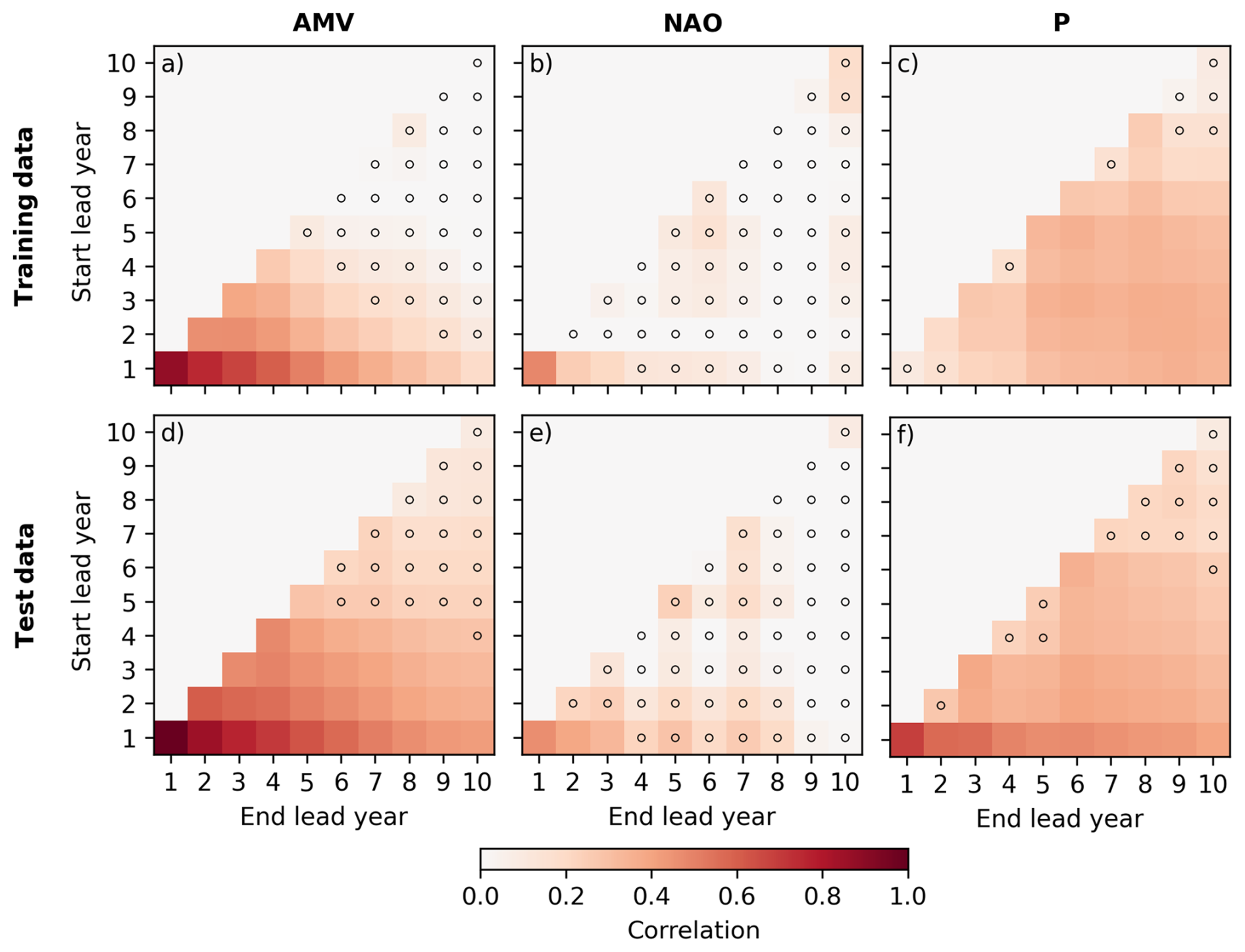
Figure 5 Model skill. The ability of the dynamical model to predict future AMV index (left column), NAO index (middle column), and North Atlantic precipitation anomalies (right column). The metric of performance is given by the correlation coefficient between model predictions and observational data. Data is split into training (first row) and test data (second row), where the training data is from ERA5 (January 1950 to December 2022) and the test data is from ERA20C (January 1900 to December 1949). Black markers (o) indicate not statistically significant correlations.

Predictive skill of the low-order model

To validate the low-order model of the North Atlantic, we assess its ability to predict the observed AMV, NAO and North Atlantic precipitation time series up to a decade ahead. The model is initialised every six months using observed monthly mean data from ERA5 training data (126 start dates between January 1950–December 2012) and from ERA20C test data (60 start dates between January 1900–December 1939). The model is integrated forward in time from each initial condition for ten years using a fourth-order Runge-Kutta scheme with a time step of one month. We validate the model separately on the training and testing data. We use the approach outlined in Athanasiadis et al. (2020) to measure the skill of model forecasts at different lead times and with varying averaging windows. The anomaly correlation coefficients (ACC) (Fig. 5) are calculated for all possible lead-year ranges (LYR) determined by the start lead-year and the end lead-year, with minimum and maximum lead times of 1 and 10 years, respectively. For example, for the initialisation year January 1950, the lead-year range LYR[2–8] represents the average of the simulated variable (or observed variable) that falls between January 1952 and December 1958. The pixel in Fig. 5 that corresponds to the lead-year range 2–8 is then the ACC between the simulated and observed variables averaged in this way, where the correlation is computed across all initialisation years. The leading diagonal of each plot in Fig. 5 shows the skill of 1-year averaged forecasts at different leads. As you move from the leading diagonal to the lower right corner, the averaging length increases, which can enhance predictable signals by removing noise.

The skill of the low-order model in predicting the AMV index is high at a lead time of 1 year for both training and testing data, with the skill slowly decreasing at longer lead times. We observe significant predictive capability of the low-order model in predicting the variability of the AMV out to a decade ahead, with improved skill in the test data (Fig. 5d). The skill in predicting the future NAO is substantially less than that of the AMV, with significant correlations up to a lead time of 3 years for 3-year averaged predictions in both testing and training datasets. The model is particularly good at predicting North Atlantic precipitation anomalies for both datasets (c, f), with noticeable improvements at greater start lead years compared to the AMV and NAO.

For the training data, the correlations at LYR[1–1] for the AMV, NAO, and precipitation are 0.86, 0.54, 0.11, respectively. For the test data, the correlations are 0.93, 0.52, 0.7, respectively. We compare the skill of the model for LYR[1–1] to a baseline forecast, which we choose here to be persistence. To calculate the persistence correlation, we correlate observations with the initial forecast states for LYR[1–1]. We find no significant differences between model forecast skill and persistence correlation for this lead year range across all variables and datasets. This suggests that, for early lead times, the model does not provide much additional predictive information beyond the memory of the initial state. However, the low-order model exhibits dominant variability on timescales of approximately 20 years and longer (see Fig. 4d, e, f). As such, the skill diagnosed here, which is limited to lead times of up to 10 years, targets timescales shorter than the intrinsic timescales of the model. Therefore, the finding that forecast skill is comparable to persistence in this range does not necessarily imply the absence of predictive skill at longer lead times and averaging windows. We also note that correctly initialising an ensemble of model forecasts greatly improves the low-order model's predictive performance at longer lead times, while also beating the persistence benchmark (not shown here).

We also calculate the explained variance of the model in LYR[1–1] for both training and test. For the training data, the explained variances at LYR[1–1] for the AMV, NAO and precipitation are 0.65, 0.10, and −6.62 respectively. For the test data, the explained variances are 0.81, −0.48, and 0.40, respectively. We note that AMV variability is well represented in both training and test data in this lead year range. However, the low-order model struggles to capture the variability of the NAO and precipitation. Similarly to the skill score mentioned above, this difference is likely due in part to the enhanced persistence of the AMV initial state. We note that the explained variability of the low-order models could allow for an estimation of the noise that should be added to the models to effectively represent the full variability. In addition, explained variance in a given lead year range could also support the model selection process.

We now have some confidence in the fidelity of the low-order dynamical model based on its ability to predict unseen data. We will now study the model to gain insight into the mechanisms of climate variability in the North Atlantic.

3.3 Mechanisms of Atlantic Decadal Variability

Past studies, based on observations and models, have highlighted the existence of robust 10–30 year variability in the North Atlantic, often referred to as Atlantic Decadal Variability (ADV) (Årthun et al., 2021). This is evident in proxy reconstructions (Chylek et al., 2011) and models (Timmermann et al., 1998; Cheng et al., 2004; Dong and Sutton, 2005; Frankcombe et al., 2010), and has been linked to the propagation of heat content anomalies along the Gulf Stream, North Atlantic current, and subpolar gyre (Nigam et al., 2018; Ruiz-Barradas et al., 2018; Menary et al., 2015). The prominent 20-year variability exhibited by our low-order model, as shown in the power spectra presented in Fig. 4, occurs consistently in all three of the observed AMV, NAO, and precipitation indices. We note that the variability of the coupled ocean–atmosphere of the North Atlantic on a similar time scale was also identified using reanalysis data in Vannitsem and Ghil (2017). We focus on this mode of variability for the remainder of this section. To extract 20-year variability of the AMV, NAO, and precipitation indices from both the low-order model simulated time series and observational time series, we use a symmetric band-pass filter between 10 and 30 years.

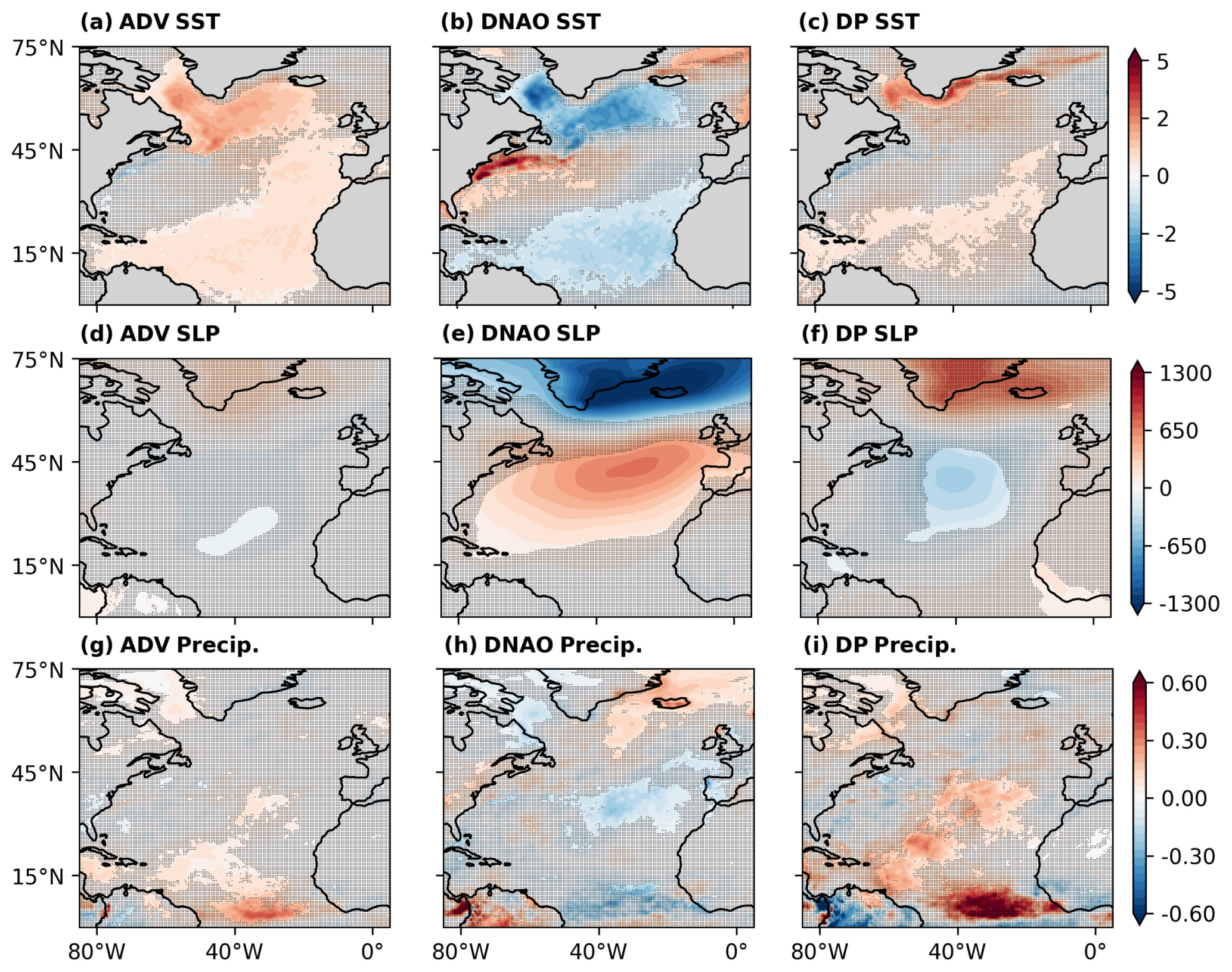
Figure 6 Decadal atmosphere–ocean variability over the North Atlantic Ocean in observations. (a–c) SST, (d–f) SLP, (g–i) total precipitation regressed onto the ADV index (first column), the DNAO index (second column), and the DP index (third column). Units are °C in (a)–(c), Pa in (d)–(f), and 10⁻² m in (g)–(i). Dots indicate where the correlation is not significant at the 95 % confidence level.

For each of the three ERA5 observed indices – AMV, NAO, and North Atlantic precipitation – we define new names for their 20-year variability components: the Atlantic Decadal Variability (ADV) index, the Decadal North Atlantic Oscillation (DNAO) index, and the Decadal Precipitation (DP) index, respectively. In Fig. 6, we perform local regressions of the observed spatial fields of monthly sea surface temperature (a–c), sea level pressure (d–f), and total precipitation (g–i) against the observed ADV index (column 1), the DNAO index (column 2), and the DP index (column 3). The SST anomalies are detrended to remove the global warming signal.

In (a), we observe that a positive ADV index is associated with particularly warm SST anomalies in the subpolar North Atlantic and weaker warm anomalies in the eastern and subtropical North Atlantic (Strommen et al., 2023). Positive precipitation anomalies associated with the ADV in (g) occur over the Labrador Sea region and in parts of the subtropical North Atlantic. The sea-level pressure regression pattern associated with the DNAO index in panel (e) is characteristic of a positive NAO loading pattern by construction (Hurrell et al., 2003). We find that the DP signal in precipitation emerges from an area around the southern node of the NAO and the subtropics, where we see positive precipitation anomalies, as shown in (i). The precipitation pattern associated with the DNAO is the familiar precipitation dipole (Walsh and Portis, 1999), characterised by an increase in precipitation over Iceland (the northern node of NAO) and a decrease over the Azores (the southern node of NAO) and the Labrador Sea. The SST pattern associated with the DNAO index is a tripole pattern (Peng et al., 2003), featuring cold anomalies in the SPNA and subtropical North Atlantic, along with warm anomalies in the subtropical gyre.

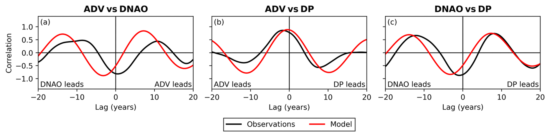
Figure 7 Lead-lag correlations of North Atlantic variables. Lead-lag correlations of (a) ADV and DNAO, (b) ADV and DP and (c) DNAO and DP indices. Black lines are computed with observed indices from ERA5 training data (January 1950–December 2022) and red lines are computed using the model simulated decadal indices over an integration time of 50 000 years.

To better grasp the interactions between variables on the 20-year timescale, we create lead-lag plots between the simulated decadal indices (ADV, DNAO, DP) and the observed decadal indices in Fig. 7. In (a), for observations (shown in black), a positive DNAO leads a positive ADV around 8–10 years later. This relationship is well understood in terms of AMV and NAO, where a positive AMV phase arises due to a delayed AMOC response to NAO-related heat-flux forcing (Delworth and Zeng, 2016; Sun et al., 2015; Delworth et al., 2017; Patrizio et al., 2025). The observed ADV and DNAO are also maximally anti-correlated near zero lag years, which is consistent with an initial cooling response of subpolar North Atlantic SSTs to anomalous wind-stress forcing associated with a positive DNAO (Fig. 6b). The low-order model's simulated DNAO-ADV relationship is similar to observations; however, the main difference is that the maximum negative correlation occurs when DNAO leads by approximately three years. Figure 7b shows a maximum positive correlation between the ADV and DP indices when the ADV leads by approximately one year. This reflects a quick response of precipitation to warmer SSTs, since a warmer ocean leads to anomalous vertical motion, thereby enhancing precipitation (Frierson et al., 2013; Sun et al., 2017; Zhao et al., 2024).

The DNAO and DP indices show a maximum negative correlation around zero lag in observations. In Fig. 6i, we observe that a positive DP index is linked to an increase in precipitation in the central North Atlantic and the southern NAO node. This is contrasted by a decrease in precipitation in the southern NAO node in response to a positive DNAO (Fig. 6h); hence, DP and DNAO are anti-correlated. The low-order model shows maximum negative correlation when DNAO leads by approximately three years. We note that the lead-lag correlations between state variables do not change significantly between candidate models with terms greater than 20 (see Sect. 2.2), which includes all stable models producing physical power spectra.

Proposed mechanisms of decadal variability in the low-order model

We hypothesise that the 20-year variability in the low-order model is a damped oscillatory mode forced by the atmosphere. The timescale is set by internal ocean dynamics, but its quasi-oscillatory nature results from decadal forcing of the NAO on the ocean state. In Zanna (2012), the existence of such a decaying oscillatory eigenmode of North Atlantic SST variability was demonstrated using an inverse linear model, with an oscillatory period of 21.1 years. However, the origin and physical mechanisms behind this mode were not specified. In this study, they also found two additional eigenmodes of variability with periods of 13.4 years and 36.8 years, which have similar timescales to the dominant peaks in the power spectra of the low-order model AMV index (15.5 years and 35 years in Fig. 4d). Further work in Zhao et al. (2017) using a LIM, identified an oscillatory mode of the North Atlantic system with a period of 19.72 years.

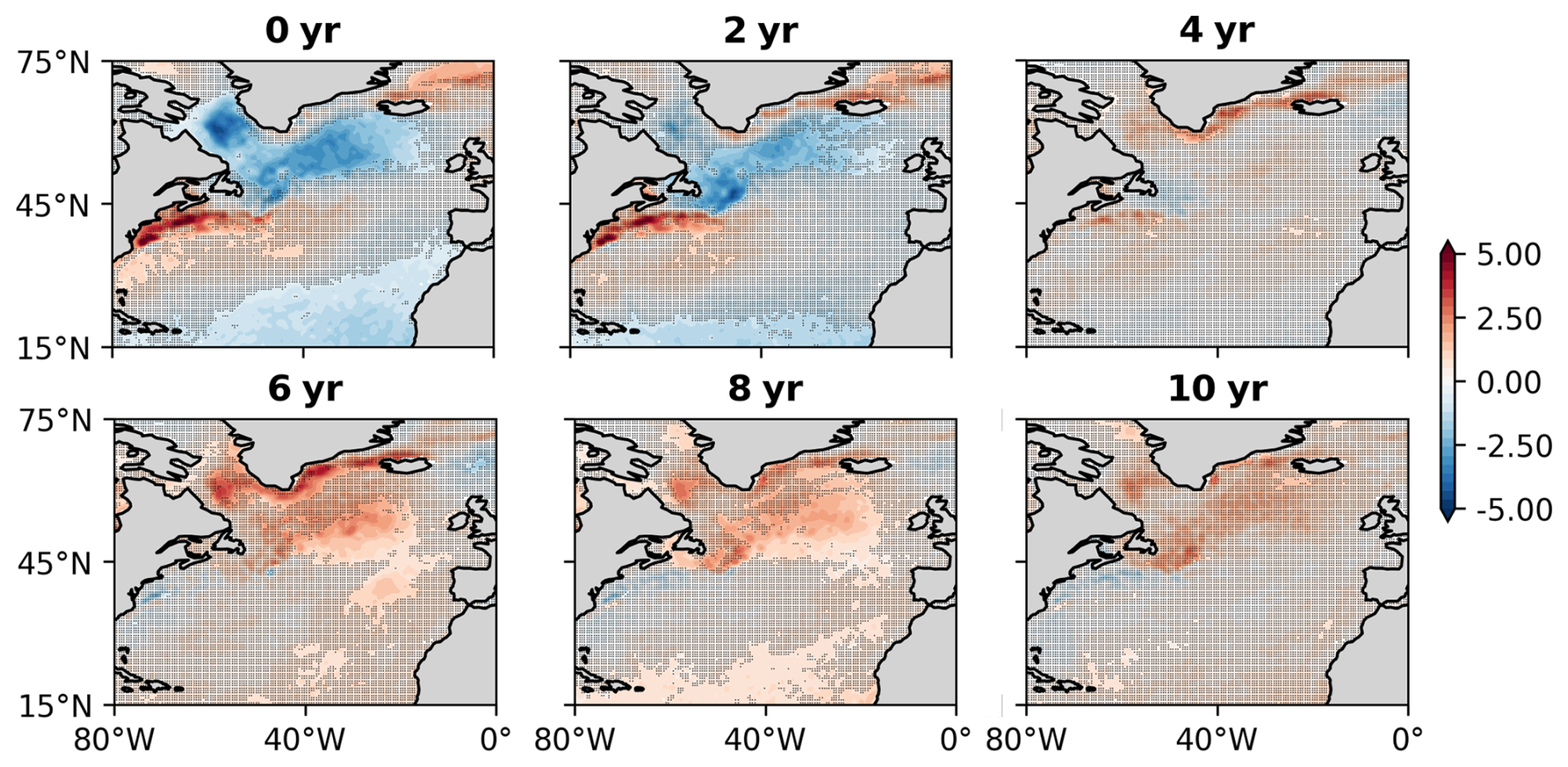
Figure 8 Sea surface temperature variability associated with the decadal NAO index. Monthly observed sea surface temperature anomalies regressed onto the observed DNAO index. The number of years represents the DNAO leading SST. Units are in °C. Dots indicate where the correlation is not significant at the 95 % confidence level.

When regressing observed SST onto the observed DNAO in Fig. 8, we see clear differences between patterns at zero lag and patterns when the SST lags. We argue that this indicates two different processes: a direct, fast response to NAO-related wind stress and heat flux forcing, followed by a slow response due to ocean adjustment of the gyre and overturning circulation. The instantaneous effect of the NAO in Fig. 8 is to cool the SPNA through anomalous wind stress, setting up a tripole pattern in SST. As we increase the lead-year of the NAO to SST, warm anomalies begin to accumulate in the SPNA and Labrador Sea regions around 6–8 years later in observations. This warming counteracts the initial cooling response of the positive NAO anomaly, thereby acting as a damping effect (negative feedback, Patrizio et al., 2025). Persistent NAO forcing on decadal timescales can give rise to an “oscillation” in sea surface temperature in the absence of other forcing. It is this slow process that has potential predictability due to the existence of an oscillation and its slow evolution. We have demonstrated that this type of quasi-decadal variability in the North Atlantic is predictable and is well captured by the low-order model (Fig. 5). The high skill of the low-order model in predicting the AMV in Fig. 5a and d directly reflects these slow, predictable ocean responses to the NAO. More importantly, the reason for the high predictive skill of North Atlantic precipitation by the low-order model (Fig. 5c) may also be attributed to these processes, as the quasi-20-year variability captured by the DP index varies in phase with the ADV index. Anomalous atmospheric convection and precipitation are direct responses to a warmer ocean. The broad 20-year peak in the observed precipitation index is similar to that of the observed AMV index in Fig. 4, reflecting a damped oscillation as the ocean integrates the atmospheric forcing.

Some studies attribute decadal ocean density changes associated with a ∼20-year mode to be driven mostly by temperature rather than salinity (Menary et al., 2015; Álvarez García et al., 2008; Zhao et al., 2017). However, in Sect. 3.1, we found that precipitation played a key role in governing the evolution of the low-order model's AMV, NAO, and precipitation indices (see Fig. 3). Here, it is plausible that the role of precipitation in the model is partly realised through freshwater fluxes (therefore modifying ocean salinity), as well as acting as a proxy for latent heating in the atmosphere. The influence of precipitation on the other variables in the low-order models arose through cross-terms of precipitation and a mode of variability. For the equations that determine the evolution of the AMV index, we found a robust dependence on the −NP terms: when the AMV is in a positive phase, and both N>0 and P>0, there is a weakening of a positive AMV towards a more neutral phase. In the case where the AMV is negative and both N>0 and P>0, the AMV tends towards a stronger negative phase. When P>0, positive rainfall anomalies emerge around the Labrador Sea (Fig. 6i) increasing flux of freshwater into the ocean. An increase in freshwater flux could lower surface salinity and increase stratification (Josey and Marsh, 2005; Myers et al., 2007), leading to a reduction in deep ocean convection and a weakening of the AMOC and the AMV (Marsh, 2000; Mignot and Frankignoul, 2003). These effects on the AMV are reinforced during a positive NAO state (N>0), as a positive NAO causes an immediate weakening of the subpolar overturning circulation due to anomalous Ekman transport. This initial weakening lasts for several months following the initial positive NAO event (Khatri et al., 2022).

For the equations that determine the evolution of the NAO index, one of the most robust terms is +NP. From this term, we find that during a negative NAO (N<0) and during positive precipitation periods (P>0), the negative NAO is reinforced by an increase in precipitation in the southern node of the NAO (see Fig. 6i) agreeing with findings from Kolstad and O’Reilly (2024). On seasonal timescales, (Kolstad and O’Reilly, 2024) demonstrated that convective precipitation in the southern NAO node is a significant mediator of the late Autumn North Atlantic SST forcing on the NAO. Diabatic heating in this region, due to enhanced convection, acts as a positive feedback on a negative NAO by lowering SLP (Rodwell et al., 1999). We also find, using the same reasoning, that a decrease in precipitation (P<0) in this region weakens a negative NAO state. We expect the response of the NAO to northern North Atlantic SST to be of opposite sign to the anomalies that induced it, in line with Patrizio et al. (2025), Delworth et al. (2017), Czaja and Frankignoul (1999, 2002), Mosedale et al. (2006). Here, the tripole SST pattern associated with a positive NAO (similar to a negative ADV SST pattern when A<0) in Fig. 6b would act as a positive feedback onto the positive NAO by enhancing the meridional temperature gradient which strengthens zonal winds and encourages a positive NAO event. If this feedback is indeed present in the low-order model, then it would have to be conditioned on the sign of North Atlantic precipitation through the +AP terms in the $\frac{\mathrm{d}N}{\mathrm{d}t}$ equations. In this case a cool SPNA and a warm subtropical gyre (associated with A<0) would reinforce the positive NAO event which induced it if the AP term is positive; which is the case when P<0. Negative precipitation anomalies in the southern node of the NAO (when P<0) are often associated with a positive NAO (Fig. 6h) and a negative ADV. Positive precipitation anomalies would favour a negative NAO and weaken a positive NAO (Kolstad and O’Reilly, 2024). Therefore, we conclude that the positive feedback pathway of North Atlantic SST onto the NAO is strongest when the North Atlantic precipitation pattern favours a positive NAO state. This highlights the importance of diabatic processes in controlling the response of the NAO to North Atlantic SST. The exact generation of the 20-year NAO variability is partly hinted at by the low-order model, with local North Atlantic SST being a strong candidate (Walter and Graf, 2002), as well as latent heating feedback mechanisms. However, further work will be required to understand these feedbacks, and the potential role of external forcing in generating North Atlantic decadal variability. Such influences on the North Atlantic atmosphere and ocean we do not consider in this study include volcanic eruptions (Swingedouw et al., 2015) and lunar cycles (Joshi et al., 2023). We note that the SINDy-derived equations in this work encode the dynamical couplings between AMV, NAO and North Atlantic precipitation, but they do not in themselves distinguish cause and effect. The mechanistic pathways we propose are supported by consistency with existing theory, but not uniquely proven by the low-order models alone. Establishing causal links will require further work.

The advance presented here lies in identifying low-order deterministic models whose nonlinear structure can reproduce key aspects of decadal variability without the need for explicitly prescribed stochastic forcing. While residual dynamics are not explicitly modelled as stochastic noise in our framework, we acknowledge that such processes are present in the real system. Some of these unresolved processes may be implicitly captured through the robust nonlinear terms identified by the low-order models. As mentioned in the discussion above, the observed coupled 20-year mode of variability is partly excited by stochastic NAO forcing and maintained by slow ocean dynamics. The “stochastic driving” of this mode of variability in the low-order models is internally generated through deterministic nonlinear interactions. A comparison of our low-order models to a Linear Inverse Model (LIM) would provide insight into whether the identified nonlinearities offer a better representation of the dynamics, allowing for improved predictive capability. We leave this as an important direction for future work. Furthermore, having these low-order dynamical models provides a tool to study the sources of decadal variability and predictability. For example, various experiments could be performed, such as suppressing terms to probe one-way couplings between equations and further parameterising the model dynamics with stochastic forcing. Further research is currently underway to study the state-dependent predictability of the low-order models and to diagnose the models' underlying physical processes by comparing them to coupled climate model simulations.

We make a final remark on the use of precipitation to represent ocean–atmosphere coupling, where we have used it as an integrated proxy for both atmospheric latent heating and freshwater fluxes. Moreover, precipitation is a useful variable from a climate impacts perspective, particularly in relation to European precipitation variability associated with the NAO and AMV. To further develop this work, one could also incorporate both sensible and latent heat fluxes, as well as freshwater fluxes, which would allow for a clearer discrimination of the role of these different processes. The SINDy algorithm can easily accommodate additional variables and higher-order nonlinearities. However, increasing the dimensionality of the models in our case introduces problems, namely the risk of overfitting on such limited observational data. Accurately disambiguating the processes linking many co-varying parameters and identifying both stable and robust models would be more challenging when working with short datasets.

4 Conclusions

There is substantial evidence that the processes linking the ocean and atmosphere in the North Atlantic, along with their feedbacks, are highly nonlinear. Many of these processes are yet to be fully understood and fully represented in climate models (Hardiman et al., 2022; García-Serrano et al., 2019; Patrizio et al., 2025). Many machine learning algorithms, such as those based on neural networks, are implicitly nonlinear and potentially useful. However, ideally, processes are represented by differential equations, as this often enables a better understanding of the system. The Sparse Identification of Nonlinear Dynamics algorithm is a suitable tool to address this problem, which we used here to derive coupled ordinary differential equations describing the temporal evolution of the coupled North Atlantic climate involving the AMV, NAO and Atlantic precipitation. The resultant low-order models derived from ERA5 reanalysis data have varying numbers of terms (including linear and nonlinear quadratic terms) and long-term behaviours. In particular, we found that models with 21 or more terms exhibit chaotic behaviour and produce broad-band power spectra in line with ERA5 observations of the AMV, NAO, and precipitation indices. The emergent variability of these models occurs strictly on decadal and multidecadal timescales, with more complex models having distinct variability of 20 years in all three state variables. We hypothesise this 20-year variability to be a damped oscillatory ocean mode, which is forced by the NAO, in line with previous findings. More importantly, we find that terms in the equations involving the multiplication of precipitation and one of the other modes of variability are among the most robust terms across the ensemble of candidate models. Upon inspection of these equation terms, we find precipitation feedbacks onto both the NAO and the AMV, and the response of the NAO to decadal AMV forcing is conditioned on the sign of precipitation anomalies. These feedbacks are consistent with diabatic atmospheric processes and freshwater fluxes represented by precipitation.

As with most methods using AI, we split the available data into training (ERA5 reanalysis) and test (ERA20C reanalysis) sets. We demonstrate that derived low-order models with 26 terms have good predictive capability at the decadal timescale on both training and unseen data. This demonstrates that diabatic processes linking the atmosphere and ocean play a crucial role in the predictability of the North Atlantic. These findings open the possibility of using the equations, correctly initialised, to estimate changes for the decade ahead. We emphasise that this could be particularly useful in predicting decadal precipitation trends in the North Atlantic and neighboring continents such as Europe and North America. Further work is currently underway, where we use the low-order dynamical model presented here to investigate error growth and predictability on decadal timescales in the North Atlantic.