Nonlinear causal dependencies as a signature of the complexity of the climate dynamics

Nonlinear quadratic dynamical dependencies of large-scale climate modes are disentangled through the analysis of the rate of information transfer. Eight dominant climate modes are investigated, covering the tropics and extratropics over the North Pacific and Atlantic. A clear signature of nonlinear influences at low frequencies (timescales larger than 1 year) is emerging, while high frequencies are only affected by linear dependencies. These results point to the complex nonlinear collective behaviour at the global scale of the climate system at low frequencies, supporting earlier views that regional climate modes are local expressions of global intricate low-frequency-variability (LFV) dynamics, which are still to be fully uncovered.

1 Introduction

During the last decades, considerable efforts have been devoted to the analysis of the low-frequency variability (LFV) in the climate system, in order to understand its origin and its implications for long-term prediction. This low-frequency variability covers a large range of timescales and processes. A first example at relatively short timescales is the succession of blocked and zonal flows, which typically covers timescales from weeks to months (e.g. Hannachi et al., 2017). Another is the low-frequency variability present in the oceans, which impact or interact with the atmosphere, which covers timescales from months to millennia (e.g. Dijkstra and Ghil, 2005). One of the most well known ocean–atmosphere interactions is the so-called El Niño–Southern Oscillation (ENSO), which occurs in the tropical Pacific with typical timescales of a few years and has considerable impact all over the globe (e.g. Alexander et al., 2002; Newman et al., 2003; Timmermann et al., 2018; Di Lorenzo et al., 2023; Stuecker, 2023). Beside this main mode of ocean–atmosphere co-variability, other low frequencies are present, covering a wide range of timescales, such as the Madden–Julian Oscillation (e.g. Wu et al., 2023), the North Atlantic Oscillation (NAO) (Barnston and Livezey, 1987) and its quasi-decadal modulation (Da Costa and De Verdiere, 2002), the Quasi-Biennial Oscillation (QBO) (e.g. Baldwin et al., 2001), the Pacific Decadal Oscillation (PDO; Mantua et al., 1997), and the Atlantic Multidecadal Oscillation (AMO; Enfield et al., 2001). These low-frequency variabilities are usually characterized through the use of some large-scale indices, which summarize the overall dynamics in specific regions of the globe.

In this context, one central question is the link between these different processes: are there drivers that dominate the overall climate dynamics, like suggested by the strong teleconnections of ENSO with the rest of the world, or is there a more intricate set of links and feedbacks that makes the dynamics more complex? Such a question is generally addressed using a process-based causal thinking which is linear by essence: assume that an observable A is modified, then B is affected, which in turn could affect C, and possibly C could affect A, inducing a feedback loop. Although this way of thinking is very useful in understanding the dynamics of a system, it is not the whole story. One can, for instance, imagine that the forcing is nonlinear or that joined (synergetic) effects of several processes could affect a third one, say through a nonlinear product A times B affecting C, which may not be isolated with the approach before. This difficulty has already been realized in climate science, as revealed by different analyses that have been performed in the past decades. A recent example is the analysis of the combined impact of the Southern Annular Mode (SAM) and ENSO on the sea ice in Antarctica (Wang et al., 2023). Another example is the dynamics of compound events which need to be activated in order to generate an extreme event (e.g. Zscheischler et al., 2018; Nguyen-Huy et al., 2018). Such types of influences are also revealed by the presence of single and cross-statistical moments of third and fourth order, for instance, between oceanic low-frequency modes (Pires and Hannachi, 2017). These findings suggest that more complicate interactions between climate modes should occur, as discussed in Wang et al. (2009), Tsonis and Swanson (2012), Wyatt et al. (2012), and Jajcay et al. (2018), in which synchronization between different climate modes was investigated. The connection between the different indices (or mode of variability) is also emphasized in de Viron et al. (2013), who showed that these modes share a common variability and a strong link with ENSO. Tackling this general problem of links between the different modes of variability necessitates both a clear picture of the (linear and nonlinear) causality involved between these modes and a clarification of the mechanisms that could be at play in such interactions.

In the current work, we focus on the first aspect by investigating the nonlinear and synergetic dependencies across a set of climate modes. A limited number of key modes is used here in order to have a tractable number of causal links to analyse and at the same time to be comparable to previous works. Eight different indices are used, as in Docquier et al. (2024a), namely the NAO, the Arctic Oscillation (AO) index, the Pacific–North American (PNA) index, the AMO, the PDO, the Tropical North Atlantic (TNA) index, the Niño3.4 index, and the QBO index. This is a similar set to that in Vannitsem and Liang (2022) without local Belgian temperature, precipitation, and insolation indices but adding the QBO. This set also corresponds to a subset of modes of Silini et al. (2022). The focus is therefore on the Atlantic, Pacific, and tropical basins of the Northern Hemisphere.

The causality analysis becomes a popular approach in climate science to evaluate the links between modes of variability. A first very interesting example is the use of the Granger causality (GC) to evaluate the influence of the sea surface temperature (SST) on the NAO (Mosedale et al., 2006). After this, the GC approach was used on many occasions, for instance, to evaluate the interaction between the ocean and the atmosphere (Bach et al., 2019). Another recent example is provided in Zhao et al. (2024), in which two versions of the GC approach are used to understand the interaction between the vegetation and the atmosphere. Several other techniques based on networks or analogues have also been tested with a lot of success; see e.g. van Nes et al. (2015), Kretschmer et al. (2016), Vannitsem and Ghil (2017), Runge (2018), Vannitsem and Ekelmans (2018), Runge et al. (2019), Di Capua et al. (2020a), Di Capua et al. (2020b), Huang et al. (2020a), and Huang et al. (2020b). Comparisons of different methods of causality analysis are provided in Krakovská et al. (2018) and in Docquier et al. (2024a), and an interesting framework, in which several measures are based on the dynamics of the information entropy, is provided in Smirnov (2022). In the current work, we use the Liang–Kleeman information flow technique (e.g. Liang, 2014a, 2016), which has been used frequently in recent years (Hagan et al., 2019; Vannitsem et al., 2019; Hagan et al., 2022; Docquier et al., 2022; Vannitsem and Liang, 2022; Docquier et al., 2023). There is, however, a crucial difference in the use of nonlinear observables (or predictors) following the work of Vannitsem et al. (2024), who showed in the context of a reduced-order nonlinear atmospheric system that the method is able to extract the influences originating from nonlinearities. As there are many possible types of nonlinear dependencies, we limit ourselves to using quadratic terms. The justification of this choice lies in the fact that many nonlinearities in fluid dynamics come from advective quadratic terms.

Section 2 describes the modes of low-frequency variability that are used in the current study. In Sect. 3, the tools used to isolate the low-frequency variability in both the atmospheric and oceanic indices and to analyse the dynamical dependencies are briefly described. The dynamical dependencies (or causality) are discussed in Sect. 4, with a detailed analysis based firstly on a reduced set of linear predictors and secondly on expanding to a set of predictors containing all quadratic products between indices. Section 5 summarizes the consequences of our findings and potential research avenues.

2 Data

Eight different regional climate indices, characterizing mostly the variability in the Atlantic and Pacific regions of the Northern Hemisphere, are considered. Four of these indices are based on atmospheric variables, and four of them are based on oceanic ones. Time series of these indices were retrieved from the Physical Sciences Laboratory (PSL) of the National Oceanic and Atmospheric Administration (NOAA; https://psl.noaa.gov/data/climateindices/list/). Monthly values from January 1950 to December 2021 are used in the present work (864 months).

The eight indices are the Pacific–North American (PNA) index (Wallace and Gutzler, 1981); the North Atlantic Oscillation (NAO) index (Barnston and Livezey, 1987); the Arctic Oscillation (AO), or Northern Annular Mode (NAM), index (Thompson and Wallace, 1998); the Atlantic Multidecadal Oscillation (AMO) index computed based on version 2 of the Kaplan et al. (1998) extended SST gridded dataset using the approach of Enfield et al. (2001); the Pacific Decadal Oscillation (PDO) index (Deser et al., 2010); the Tropical North Atlantic (TNA) index (Enfield et al., 1999); the Niño3.4 index (for the remainder of the paper, we mostly refer to this index as “Niño3.4”); and the Quasi-Biennial Oscillation (QBO) index (Graystone, 1959). These indices are the same as the ones used in Docquier et al. (2024a), in which more details on their characteristics may be found.

3 Methods

3.1 Singular spectrum analysis (SSA)

Singular spectrum analysis (SSA) shows similarities with the principal component analysis where a covariance matrix is diagonalized. In SSA, the lag-covariance matrix of a single time series is diagonalized where the eigenvectors or temporal empirical orthogonal functions (T-EOFs) are finite time sequences providing the more frequent and higher-amplitude finite time spells of that variable. To construct them, the time series X(i) with $i=\mathrm{1},\mathrm{\dots },N$ of each index is embedded into a phase space of dimension, say M, using a delay-coordinate state vector $Y\left(t\right)=\left[X\right(t-M+\mathrm{1}),\mathrm{\dots },X(t\left)\right]$, whose coordinates are the successive values in the time series (e.g. Broomhead and King, 1986; Vautard et al., 1992; Fraedrich et al., 1993; Ghil et al., 2002). The evolution in phase space is then obtained by sliding the M window in time. This operation can be expressed as an eigenvalue problem of the following M×M Toeplitz matrix:

$$\begin{array}{}\text{(1)}& \left(\begin{array}{ccccc}T\left(\mathrm{0}\right)& T\left(\mathrm{1}\right)& T\left(\mathrm{2}\right)& \mathrm{\dots }& T(M-\mathrm{1})\\ T\left(\mathrm{1}\right)& T\left(\mathrm{0}\right)& T\left(\mathrm{1}\right)& \mathrm{\dots }& T(M-\mathrm{2})\\ \mathrm{\dots }.\\ T(M-\mathrm{2})& T(M-\mathrm{3})& T(M-\mathrm{4})& \mathrm{\dots }& T\left(\mathrm{1}\right)\\ T(M-\mathrm{1})& T(M-\mathrm{2})& T(M-\mathrm{3})& \mathrm{\dots }& T\left(\mathrm{0}\right)\end{array}\right),\end{array}$$

where each matrix entry (i,j) is the lag covariance $cov\left(X\right(t),X(t+|i-j|\left)\right)$. The eigenvalues and eigenvectors can then be computed. These eigenvectors characterize the dominant modes within the M window, such as intermittent oscillating spells with periods less than M. The window M is generally fixed to $\mathrm{1}/\mathrm{10}$ of the length of the time series in order to have enough statistics for estimating the covariance matrix. In the current work, it is fixed to 240 months, a bit longer than the default value, in order to resolve decadal timescales. More information on the method is provided in Vautard et al. (1992) and Ghil et al. (2002).

For each index, we compute the SSA spectrum and visually evaluate each of the 40 SSA modes corresponding to the 40 dominant eigenvalues. These different modes have a time length of 240 months (the M window mentioned earlier). If the dominant period in each mode evolution is shorter than 1 year, the mode is discarded, the idea being to keep the low-frequency variability larger than 1 year. After filtering out the modes displaying high frequencies, we end up with new low-frequency-variability series of the original monthly anomalies of the climate indices (the monthly mean is removed before the application of SSA). The modes that are kept at a low-frequency signal are listed in Table 1. Here, there is a certain degree of arbitrariness, as we sometimes discard modes that display a mix of low-frequency and high-frequency variabilities. We do believe, however, that the essence of the LFV dynamics is captured well by our selection. Note also that the LFV of most of the oceanic modes is essentially concentrated on the dominant SSA modes of variability.

Table 1 Set of SSA modes kept in the reconstruction of the low-frequency variability of the monthly anomalies of the climate indices displayed in Fig. 1.

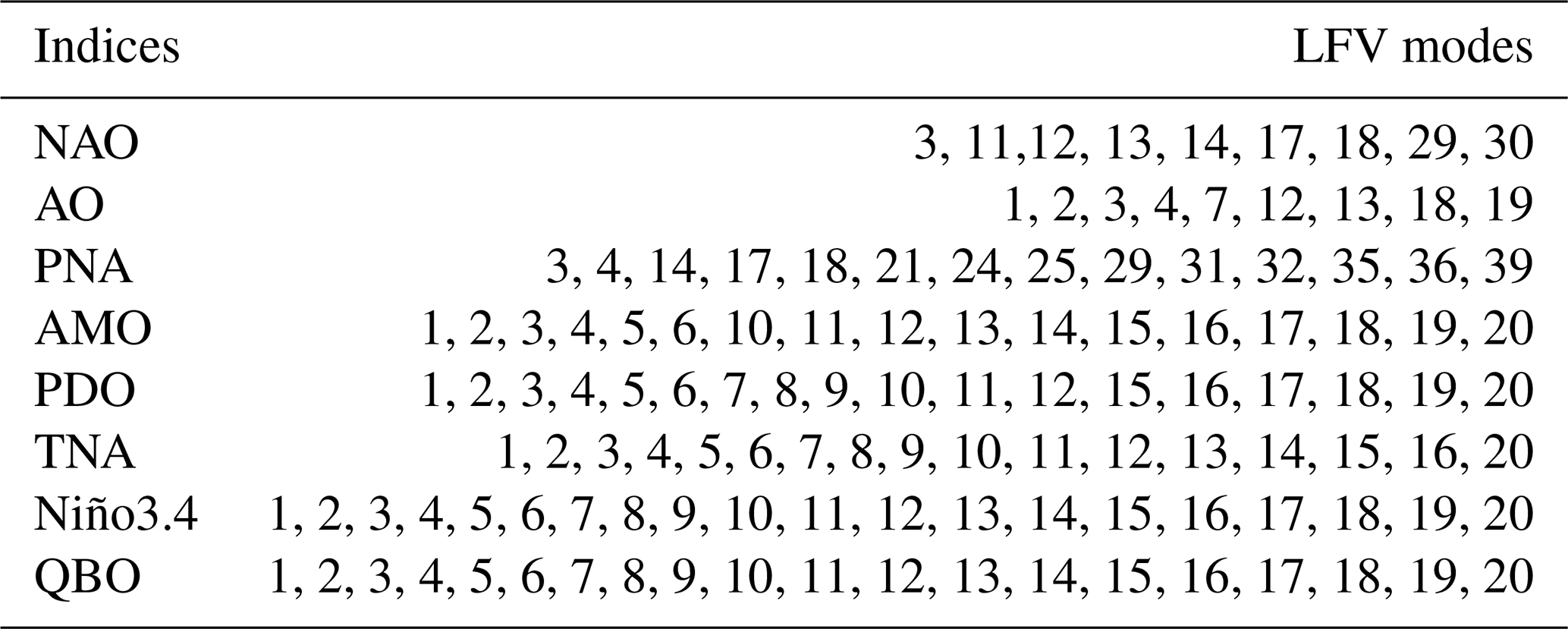
In order to evaluate the impact of choosing specific SSA modes rather than others on the causality analysis, we also considered arbitrary choices of modes, namely the even modes 2k and the odd modes $\mathrm{2}(k-\mathrm{1})+\mathrm{1}$, for $k=\mathrm{1},\mathrm{\dots },\mathrm{20}$. The analysis reveals that considerably fewer significant influences from nonlinearities are detected (five instances for the odd modes and two instances for the even modes), indicating that these arbitrary choices do not provide optimal results. With such choices, high and low frequencies are again mixed up, leading to a rather suboptimal result. The presence of high frequencies indeed hinders the proper detection of dependencies given the short time series.

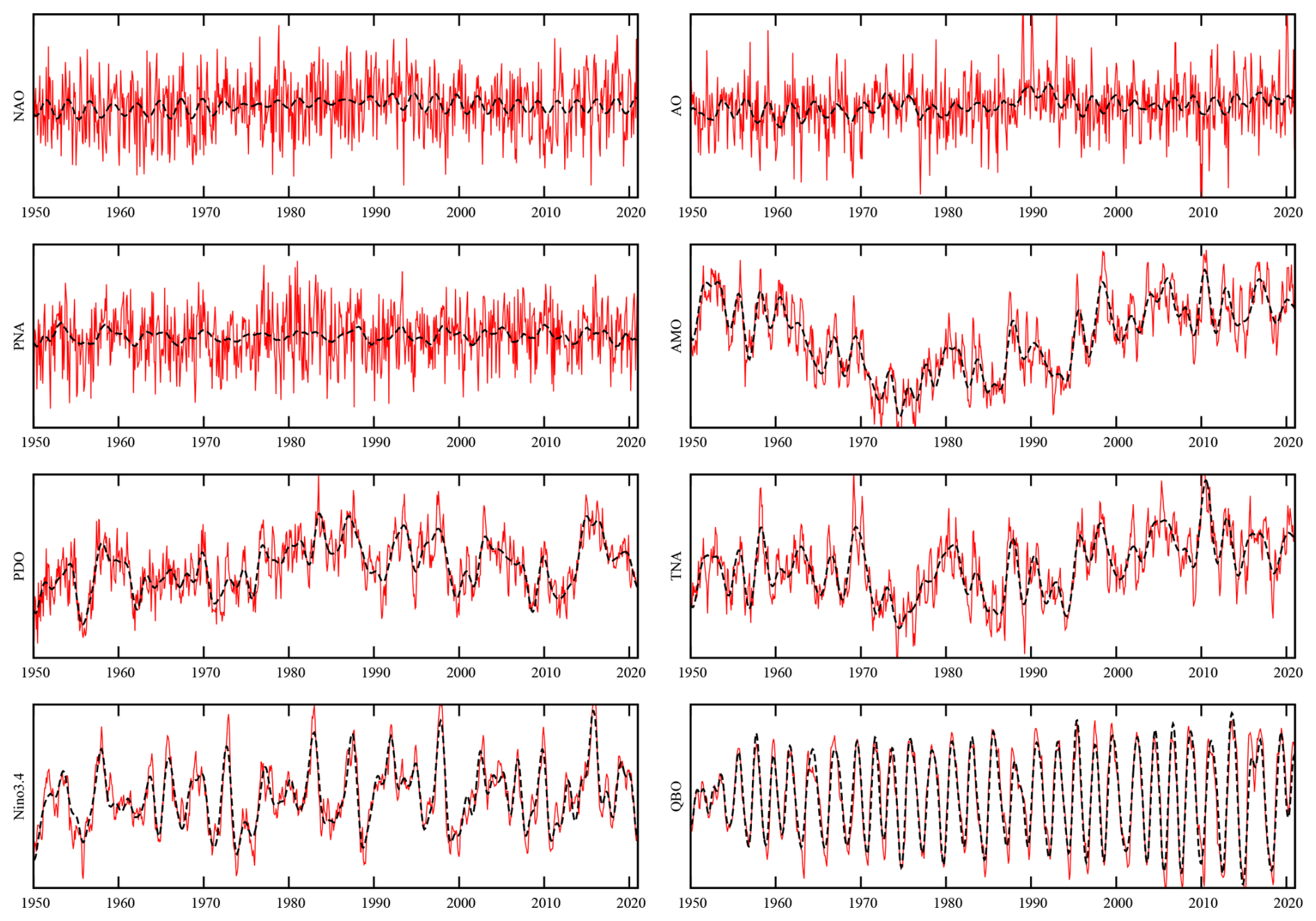
Figure 1 Original (red) and filtered (black) monthly anomaly time series of the climate indices, covering the period 1950–2021.

Note that a sensitivity test was also performed by removing the trends in temperature for the Niño3.4 index, with little impact on the results discussed below.

3.2 Rate of information transfer

Liang developed a theory on causal dependencies in the context of nonlinear stochastic systems based on the estimation of changes in the information entropy of the system, leading to an expression for the rate of information transfer between variables (Liang and Kleeman, 2005; Liang, 2014a, b, 2016, 2021). A simpler expression was subsequently deduced for linear stochastic systems forced by additive noise, allowing direct estimation with observational data as discussed in Liang (2014b, a, 2021). The latter approach is also known as the Liang or Liang–Kleeman method. It has been applied in various climate contexts (Vannitsem et al., 2019; Vannitsem and Liang, 2022; Docquier et al., 2022, 2023, 2024a). A recent extension of the theory allowing the estimation of the rate of information transfer based on conditional expectations was performed in Pires et al. (2024) and tested in the context of a reduced-order model displaying deterministic chaos in Vannitsem et al. (2024). In the latter, an extension of Liang's method for time series analysis is also tested to allow the incorporation of nonlinear predictors.

Let us consider the S time series, X_i, $i=\mathrm{1},\mathrm{\dots },S$, having N data points, X_i(n), $n=\mathrm{1},\mathrm{2},\mathrm{\dots },N$, recorded at a regular time step Δt. A forward temporal derivative can be computed as

$$\begin{array}{}\text{(2)}& {\dot{X}}_i\left(n\right)={\displaystyle \frac{X_i(n+\mathrm{1})-X_i\left(n\right)}{\mathrm{\Delta }t}}.\end{array}$$

Let us denote C_ij as the sample covariance between X_i and X_j and C_i,dj as the sample covariance between X_i and the temporal derivative ${\dot{X}}_j$. It has been shown that the estimator of the rate of information transfer from variable X_j to variable X_i is

$$\begin{array}{}\text{(3)}& {\widehat{T}}_{j\to i}={\displaystyle \frac{\mathrm{1}}{\det \mathbf{C}}}\cdot \sum _{k=\mathrm{1}}^S{\mathrm{\Delta }}_{jk}{C}_{k,di}\cdot {\displaystyle \frac{C_{ij}}{C_{ii}}},\end{array}$$

where Δ_jk are the co-factors of the covariance matrix C=(C_ij) and detC is the determinant of C. Note that this is valid under the approximation that (X_i,X_j) is jointly Gaussian, otherwise the term $C_{ij}/C_{ii}$ must be replaced by $E[\mathrm{d}/\mathrm{d}{X}_i(E\left(X_j\right|X_i\left)\right)]$, relying on nonlinear conditional expectations as in Pires et al. (2024).

Generically, causation is assumed to imply correlation, but correlation clearly does not imply causation. This feature emerges nicely in the mathematical expression (3) when considering two time series only as discussed in Liang (2014a), so the significance test allowing the evaluation of causal dependencies consists of computing the rate of information transfer and checking whether it is significantly different from zero. Several approaches may be used, and here a bootstrap method with replacement is used (Efron and Tibshirani, 1993) in a similar way to that in Vannitsem et al. (2019). The level of confidence is fixed here to 1 % in order to avoid a false positive as far as possible, but, as indicated in Docquier et al. (2024a), a false negative may arise when the number of predictors is high and the time series is short. This caution is most probably applicable here; therefore some nonlinearities may not be properly isolated (some false negative).

A normalization of the rate of information transfer is also performed in such a way that the influences of the different variables on the target can be evaluated on the same grounds. It provides a percentage of influence. The normalization factor in the multivariate case is the same as in Liang (2021):

$$\begin{array}{}\text{(4)}& Z_i=\sum _{k=\mathrm{1}}^S\left|{\widehat{T}}_{k\to i}\right|+\left|{\displaystyle \frac{\mathrm{d}{H}_i^{\mathrm{noise}}}{\mathrm{d}t}}\right|,\end{array}$$

where $\left|\frac{\mathrm{d}{H}_i^{\mathrm{noise}}}{\mathrm{d}t}\right|$ is the contribution of the noise of the underlying linear stochastic model.

The relative transfer of information from X_j to X_i is given by

$$\begin{array}{}\text{(5)}& {\mathit{\tau }}_{j\to i}={\displaystyle \frac{{\widehat{T}}_{j\to i}}{Z_i}}.\end{array}$$

Note that the time series used are relatively short. This implies that some links could not be detected, as the uncertainty around the value of the rate of information transfer may be large. Given that caveat, some dependencies of the method on the bootstrap sample are explored in Docquier et al. (2024a). They concluded that 1000 bootstrap samples are a good choice to detect causal links in short climate time series.

Another potential difficulty is the number of predictors. In Docquier et al. (2024a), it was indicated that, to obtain good detection, a small number of predictors should be used (of the order of maximum 10). It was, however, shown in the more theoretical study of Vannitsem et al. (2024) that using a combination of linear and nonlinear terms up to 44 predictors still allows us to obtain meaningful results. The different conclusions reached are probably associated with the different setups used in both studies, and this question should be further addressed in the future.

The approach proposed by Liang allows the construction of a network of directional connections between observables that are measured concomitantly. This approach is distinct from techniques that assume that causation should be based on a time lag between events, such as the classical network approach (Runge et al., 2019; Di Capua et al., 2020a). If real processes indeed display a lag (like in the propagation of a wave), the information will propagate from one point to another, and this will be isolated in Liang's method through a specific path through the network. In reality, as we usually do not have all variables (at all grid points, for instance), this could not show up, but filtration through (spatial or temporal) averaging or frequency selections should help to disentangle the impact of one distant observable on another, as, for instance, in Vannitsem and Liang (2022).

Note also that the sign of influence also contains interesting information: when positive, it means that the predictor is inducing an increase in the uncertainty (or variability) of the target, while, when it is negative, the predictor reduces the uncertainty (variability) of the target. This information is, however, quite sensitive to the set of predictors used, as discussed in Vannitsem et al. (2024). We therefore do not discuss this in detail, except if outstanding features are emerging.

4 Results

4.1 Influence on an atmospheric index: NAO

Let us first consider the influence on one specific climate index, the NAO. Figure 2 displays the application of Liang's method (Eq. 5) to the original NAO time series and to the low-frequency filtered data. A first remark is that the only influence detected at the 1 % level in the original series originates from the AO, while correlation is statistically significant for the AO, AMO, and TNA. This result is in agreement with Docquier et al. (2024a). Note that we use 1 % in order to reduce false positive cases, particularly when the number of predictors used is large. When the analysis is applied to the low-frequency variability of the series, the influence of the AO does not appear anymore, while the influence of the PNA and QBO emerges, together with correlations with all the other indices. The fact that the AO influence disappears probably reflects that it mostly acts on shorter timescales (not present in the LFV series anymore), while the PNA and QBO emerge in the low-frequency NAO signal. The influence of the TNA is consistent with the barotropic teleconnection mechanism proposed in Okumura et al. (2001).

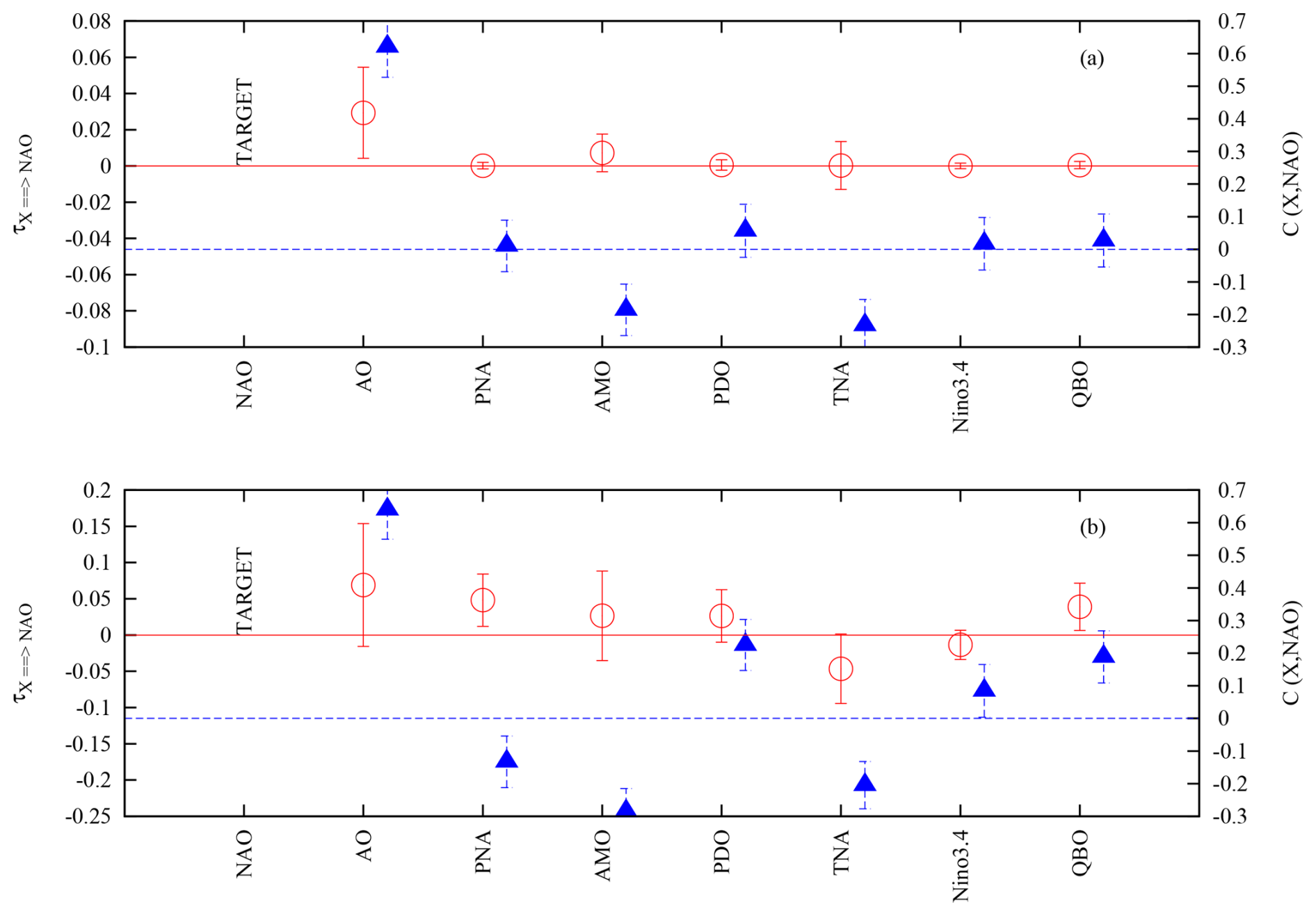
Figure 2 The rate of information transfer (left y axis, red open circles) and the correlation (right y axis, blue triangles) are plotted as functions of the observables for the targeted observable (labelled TARGET in the plot): the NAO. Panels (a) and (b) are for the original and LFV time series, respectively.

This linear approach could, of course, miss the impact of the joint influence or co-variability of indices. In Vannitsem et al. (2024), this question was addressed in the context of a reduced-order atmospheric model, and it was shown that joint influences in the form of polynomial nonlinearities could be very large and dominate the sources of information transfer. To deal with that aspect in the context of time series analysis, they also propose to use new types of observables in the context of Liang's approach as products of system variables. It was indeed found that, if nonlinearities do not play a role in the dynamical equations, the corresponding rate of information transfer obtained from the time series generated by the model would be negligible. This result provides some hope of also being able to isolate nonlinear influences in the real atmosphere and in the climate system.

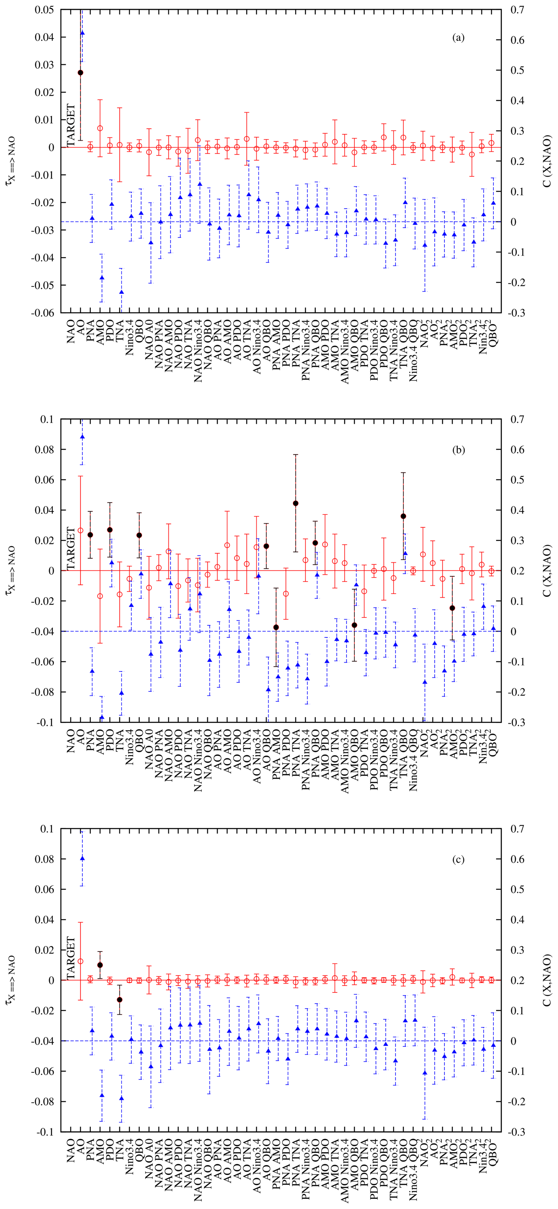
Figure 3 The rate of information transfer (left y axis, red open circles) and the correlation (right y axis, blue triangles) are plotted as functions of the observables for the targeted observable (labelled TARGET in the plot): the NAO. Panels (a), (b), and (c) are for the original, the LFV, and the high-frequency time series, respectively. The observable set is composed of 7 linear terms and 36 nonlinear quadratic terms, all listed along the x axis. The points in black refer to the significant dependencies at the 1 % level.

To disentangle the role of nonlinearities in the context of the eight climate indices, all combinations of quadratic terms are constructed. This choice is made, since, in many dynamical systems, such nonlinearities are present. These quadratic nonlinearities are typically associated with the presence of nonlinear advection terms in the classical conservation laws (momentum equation, thermodynamic equation, etc.), for instance, as illustrated in the work done recently in the context of the Charney–Straus model (Vannitsem et al., 2024). However, these could be viewed as restrictive, and tests should be done in the future to evaluate the impact of higher-order or more complicated nonlinearities.

Figure 3a displays the application of Liang's approach with the additional 36 quadratic observables in the original series. The only influence emerging in this panel is associated with the AO index, as in the analysis based on the purely linear approach of Fig. 2. It is striking to see that there is no quadratic nonlinearity which emerges here, as these observables are very close to 0. This negative result is very useful, as it shows that, if there is no nonlinear influence in the form considered here, it will not show up and that the linear dependence on the AO is a robust feature of the influence on the NAO in the original series.

An even more striking result is found when only investigating the low-frequency variability of these indices. Figure 3b displays the results with the nonlinear observables. As with the previous discussion of Fig. 3a, the dependencies of the NAO from the PNA and QBO again emerge, but additional dependencies are found from the PDO and seven different nonlinearities: PNA TNA, TNA QBO, PNA AMO, AMO QBO, AMO², PNA QBO, and AO QBO. In all those cases, correlation is significantly different from zero, though the reverse is not true, as expected (i.e. correlation does not imply causation). The PDO influence on the low-frequency variability of the NAO is consistent with the findings of Nigam et al. (2020). The influence of the QBO is also consistent with the important role played by the stratosphere, as found in Ambaum and Hoskins (2002) and Scaife et al. (2005). This indicates that the influence of the Atlantic Ocean through the TNA and AMO is only emerging jointly with the PNA and QBO and through the quadratic amplitude of the AMO. At the same time, the influence of the AO is now mediated through the joint influence with the QBO. Interestingly, the nonlinear joint influence of the QBO with the Atlantic multidecadal variability is consistent with the results presented in Omrani et al. (2014, 2022), who demonstrated the essential influence of the stratosphere on the extratropical atmospheric response to ocean variability. The latter interesting investigation of joint influences, consistent with our findings, should be extended to the other nonlinearities uncovered in the current analysis. A visual picture of the dependencies is provided in Fig. 4.

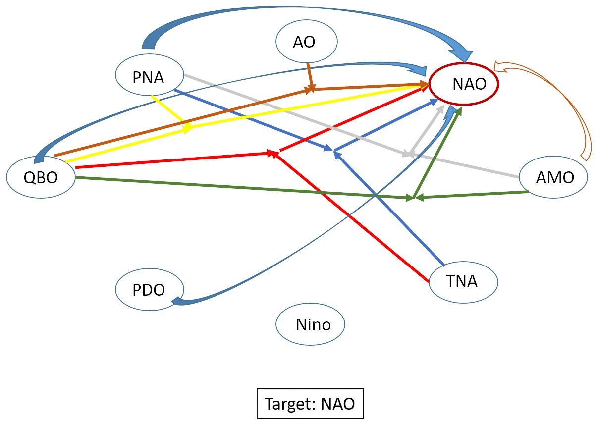
Figure 4 A visual representation of the linear and nonlinear influences from the set of indices on the NAO for the low-frequency-variability dataset. The curved plain arrows refer to the linear influence, and the triple straight arrows with the same colours refer to the influence of the quadratic nonlinearities: two straight arrows emanate from two indices, joining somewhere in between the indices, and from there the third straight arrow indicates the target.

Related to the sign of influence, it is interesting to note that all nonlinear predictors involving the AMO show a negative influence on the NAO. This feature suggests that the AMO, in combination with several indices, tends to reduce the variability of the NAO. This conjecture should be checked in the future, either through additional analyses with a wider set of indices or through a process-based analysis, as done, for instance, in Omrani et al. (2014, 2022).

A test on the high-frequency variability computed as the difference between the original series and the LFV series is also performed to clarify whether nonlinearities also play an important role at these frequencies. Two weak linear dependencies emerge from the AMO and the TNA, suggesting some quick response of the NAO to the Atlantic Ocean temperature, but no nonlinear influences emerge here. This interesting feature suggests that nonlinear couplings between the different climate modes are only present at long timescales. This point is also taken up in the next section.

Here, a few important considerations are in order:

• As in Vannitsem et al. (2024), the use of new nonlinear observables could also modify the contributions of linear influences, such as the emergence in Fig. 3b of the influence of the PDO and the reduction in the TNA influence in the low-frequency NAO signal. The modifications can either be present in the average influence or in the amplitude of the confidence intervals.

• A few influences in the low-frequency variability of climate indices could emerge only through nonlinearities, revealing the joint impact of pairs of indices.

• The high-frequency variability of the NAO is only influenced through linear terms associated with the ocean variability over the Atlantic.

• The fact that the use of nonlinear terms in the original and high-frequency series does not provide any substantial influence suggests that the scheme proposed is unlikely to produce spurious influence through nonlinear terms if indeed not present.

4.2 Influence on an oceanic index: El Niño

Let us now perform the same analysis for the well-known dynamics in the tropical Pacific. Figure 5a shows the influence at the 1% level of confidence of the PNA and TNA; again, this is in agreement with Docquier et al. (2024a). If one considers the low-frequency variability only, the influence of the PNA is not statistically significant at the 1 % level but is significant at the 5 % level. On the other hand, there is a very strong influence of the TNA and PDO with amplitudes of −0.181 and −0.163, both accounting for more than 35 % of the total influence. Both characterize ocean processes known to be connected with the dynamics of El Niño (Levine et al., 2017; Park and Li, 2019; Johnson et al., 2020).

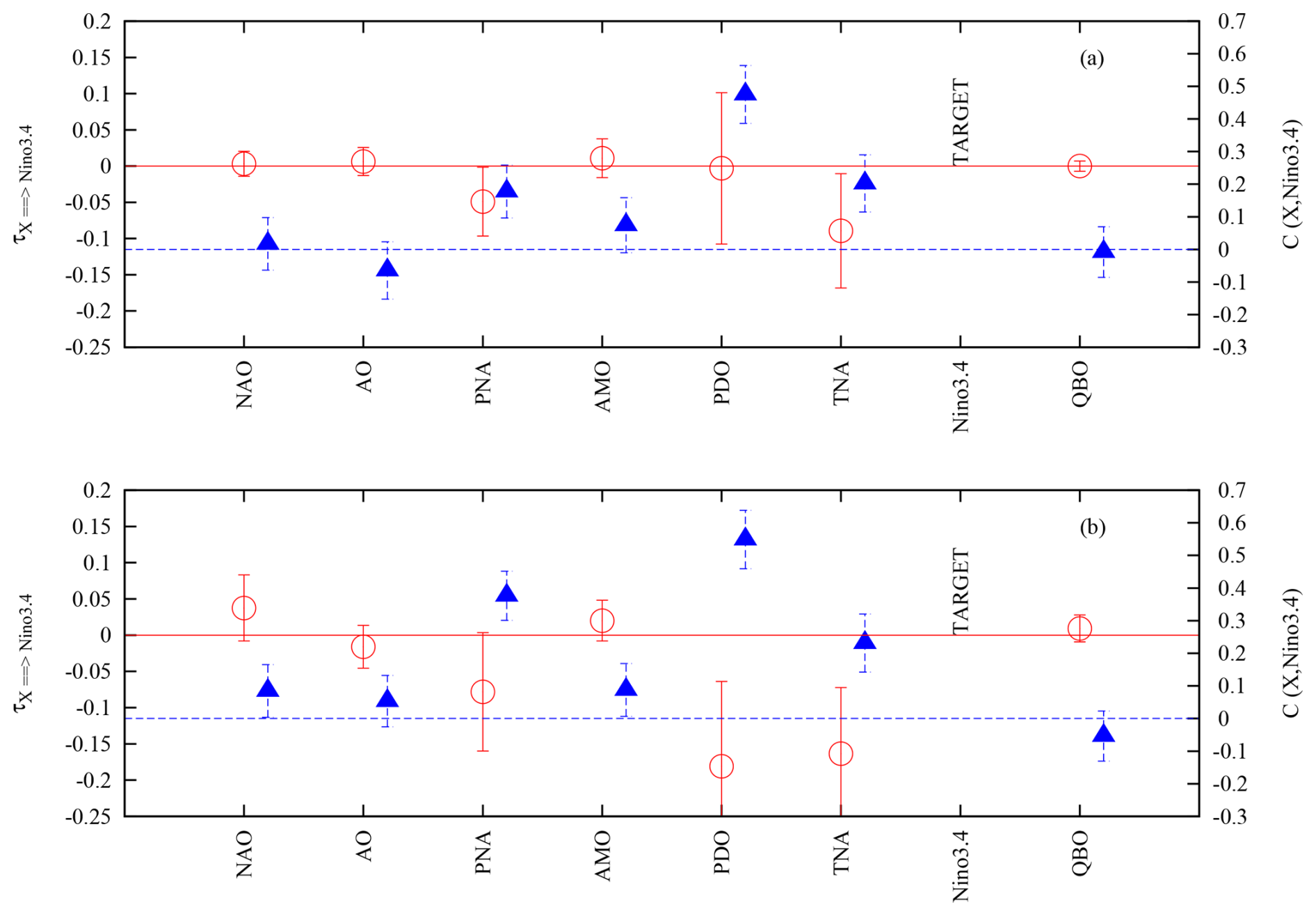
Figure 5 The rate of information transfer (left y axis, red open circles) and the correlation (right y axis, blue triangles) are plotted as functions of the observables for the targeted observable (labelled TARGET in the plot): Niño3.4. Panels (a) and (b) are for the original and LFV time series, respectively.

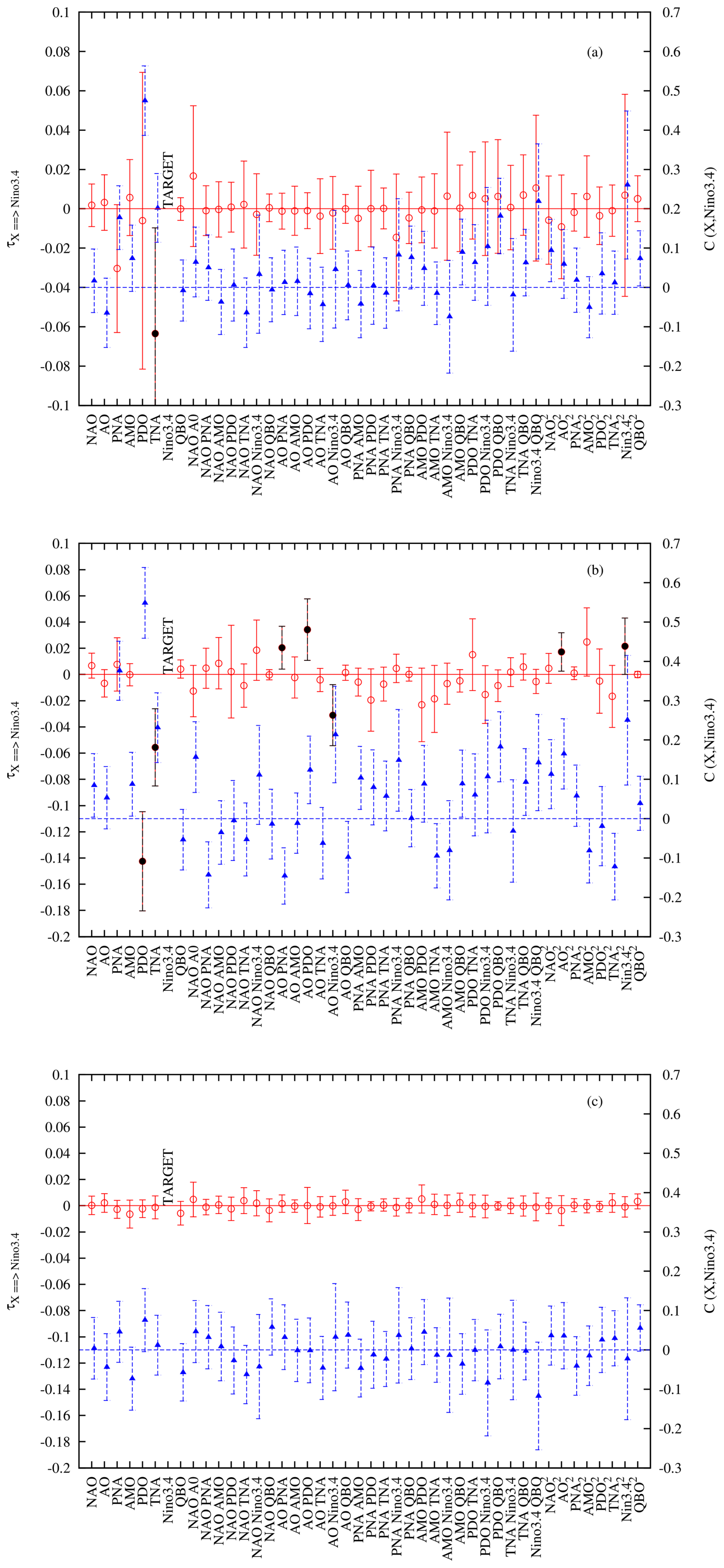
Figure 6 The rate of information transfer (left y axis, red open circles) and the correlation (right y axis, blue triangles) are plotted as functions of the observables for the targeted observable (labelled TARGET in the plot): Niño3.4. Panels (a), (b), and (c) are for the original, the LFV, and the high-frequency time series, respectively. The observable set is composed of 7 linear terms and 36 nonlinear quadratic terms, all listed along the x axis. The points in black refer to the significant dependencies at the 1 % level.

Figure 6a displays the analysis done with all the quadratic nonlinearities. Firstly, there is no specific nonlinearity which emerges here. Secondly, the dominant influence is now in the TNA at the 1 % level, while the PNA will only appear at a lower level of confidence. As for the NAO, the extension of the analysis of the original series using the nonlinear terms did not show any nonlinear influence and only revealed the influences already isolated with the original variables.

Let us now turn to the nonlinear analysis of the low-frequency series (Fig. 6b). The influences of the PDO and TNA still remains dominant, although with lower amplitudes. Interestingly, most of the nonlinearities that show significant influence (AO PDO, AO Niño3.4, AO PNA, AO²) involve the influence of the AO; the only additional nonlinearity is Niño3.4². This influence clearly does not emerge in the purely linear analysis, suggesting that the AO influences the low-frequency variability of El Niño only in conjunction with other key climate indices. To our knowledge, this specific influence of the AO on El Niño was not reported before, which is worth exploring further in the future. The additional positive causation comes from the nonlinear term Niño3.4², which is related to the positive El Niño skewness (Burgers and Stephenson, 1999) and the tendency for extreme El Niños or La Niñas to generate future El Niños, 2–3 years later, as shown by cross-bicovariance and bi-spectral analysis of El Niño time series (Pires and Hannachi, 2021). A visual picture of the dependencies on Niño3.4 is provided in Fig. 7.

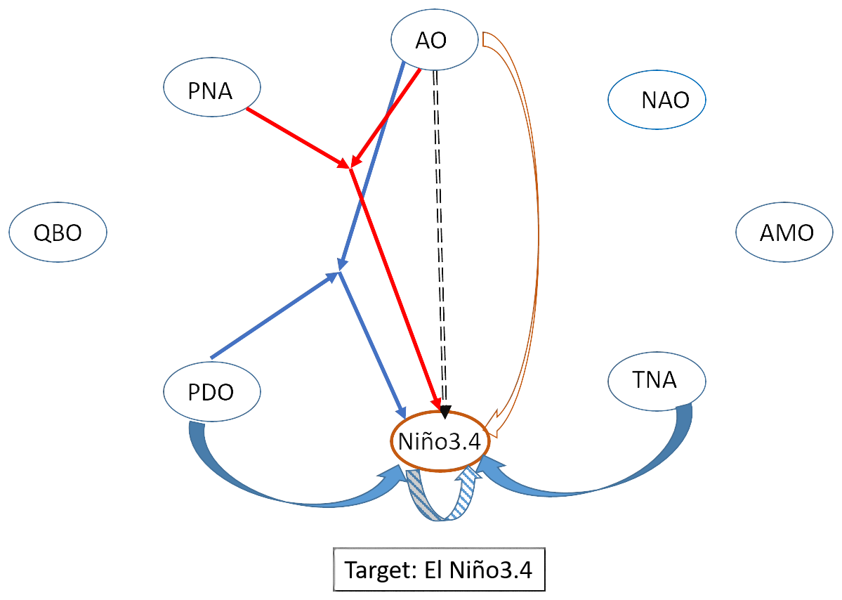
Figure 7 A visual representation of the linear and nonlinear influences from the set of indices to Niño3.4 for the low-frequency-variability dataset. The curved plain arrows refer to the linear influence, and the triple straight arrows with the same colours refer to the influence of the quadratic nonlinearities: two straight arrows emanate from two indices, joining somewhere in between the indices, and from there the third straight arrow indicates the target. The double-dashed straight (black) arrow indicates the influence of the product between the source and the target. The empty curved arrow indicates the quadratic influence of the source, while the striped curved arrow indicates the quadratic influence of the target.

Interestingly, there is no influence of any linear or nonlinear predictor at high frequencies as illustrated in Fig. 6c. This result firstly demonstrates that only low-frequency variability in the other indices influences the dynamics of Niño3.4 and secondly, on more technical grounds, that a false positive can indeed be rare, giving confidence in the analyses done on the low-frequency-variability indices. Similar remarks to the ones listed at the end of the previous section are also in order here.

4.3 Influences on the other climate modes

Concerning the other indices, a similar analysis was performed, and a summary of the findings is given in Tables 2 and 3 for the analysis based on the eight original filtered series only and based on the extended set of observables containing the 8 variables themselves and the nonlinearities already described in the previous sections. Note that all detailed figures are given in the Supplement.

Table 2 List of climate indices that have a significant influence on the targets mentioned in the first row. These are listed by order of importance based on the mean value of the rate of information transfer (over 1000 bootstraps). These estimates are shown in Figs. 2 and 5 and in the figures in the Supplement. The value for the dominant information transfer is given between parentheses.

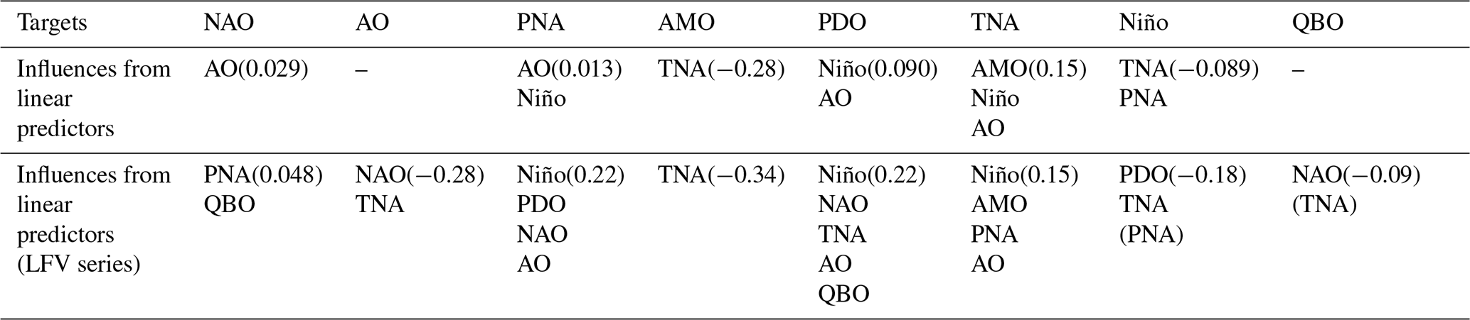
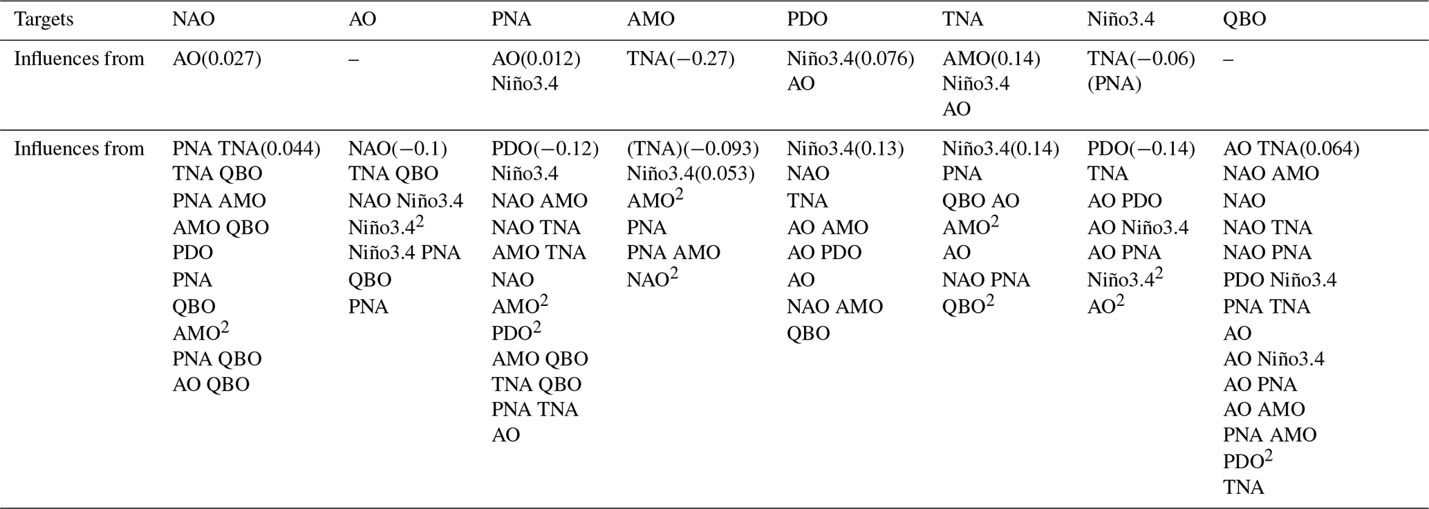
Table 3 List of climate indices and their quadratic products that have a significant influence on the targets mentioned in the first row. These are listed by order of importance based on the mean value of the rate of information transfer (over 1000 bootstraps). These estimates are shown in Figs. 3 and 6 and in the figures in the Supplement. The value for the dominant influence is given between parentheses. In the first row, the results with the use of 44 predictors in the original series are displayed, while, in the second row, the results with 44 predictors in the LFV series are displayed. Note that, for the AMO, the influence of the TNA in parentheses with the set of nonlinear predictors is still intense, but only at the 5 % level.

For the AO, there is no influence detected on the original series. Turning now to the filtered ones containing the low-frequency variability of all series, the linear analysis reveals the presence of influence of the NAO and TNA. If one uses all nonlinearities, the influence of the NAO still remains a linear term, but that of the TNA does not. The TNA now appears in conjunction with the influence of the QBO. Niño3.4 also emerges through the nonlinearities in conjunction with the NAO and PNA. Finally, the QBO and PNA are also emerging as influencing the AO linearly.

The PNA is influenced by Niño3.4 (as also indicated in Silini et al., 2022) and the AO, whatever the original or filtered series, is analysed, whatever the set of predictors used (linear or nonlinear). This shows the robustness of these influences for both the full-variability series and its low-frequency counterpart. When the nonlinear analysis is performed on the filtered series, a large set of new influences emerges: the PDO as the dominant influence which was not present in the linear analysis; the NAO with a linear influence; and a bunch of nonlinear influences involving the NAO, AMO, TNA, PDO, and QBO. Here, all indices show influences either through linear or nonlinear terms. This reflects the complexity of the dynamics of the PNA.

The AMO shows an overall strong influence from the TNA, whatever the series and predictor sets used. When the nonlinear analysis of the filtered series is performed, a set of linear and/or nonlinear influences emerges from the PNA and NAO, together with a quadratic self-influence. Interestingly, a strong NAO is likely to influence the AMO through the term NAO², revealing the importance of extreme NAO events on the AMO, while the influence of the PNA emerges only in conjunction with an amplification of the AMO.

For the PDO, the influences of Niño3.4 and the AO are always detected in the different analyses performed. The analysis confirms results already reported in Silini et al. (2022) and Vannitsem and Liang (2022). When the filtered data are used, additional linear influences are detected from the TNA, NAO, and QBO, together with some nonlinear dependencies combining the AO, NAO, AMO, and PDO.

For the TNA, a similar picture is found, with influences from Niño3.4, the AMO, and the AO found in all analyses performed, either linear or nonlinear or using the original or filtered data. The influence of the PNA emerges only in the analysis of the filtered dataset, and additional influences from the QBO and PNA are felt through nonlinearities. Note also that the AMO does not appear as a linear influence in the fully nonlinear analysis of the filtered data, but rather as the square of this index. The latter reveals that a strong influence of the AMO is only felt when the AMO has high amplitude.

Finally, for the QBO, no influences are felt using the original dataset, while they appear on the filtered data, with a dominant influence of the NAO in the linear analysis. For the fully nonlinear analysis, a large variety of nonlinearities influence the QBO in which all climate modes are involved. Note, however, that these influences are always very small, even if significant.

The analysis based on the high-frequency time series reveals that there are no nonlinear influences affecting the different indices: For the NAO, weak influences on the AMO and TNA are detected; for the AO, there is a weak influence of the TNA; for the PNA, there are weak influences of the AO and PDO; for the AMO, there is a large influence of the TNA; for the PDO, there is a weak influence of the AO; for the TNA, there are influences by the AO and AMO; and, finally, for the QBO, there is no influence detected.

All these complicated nonlinear dependencies between the climate modes are also worth exploring more from a process dynamics perspective, as was done for the interaction between the stratosphere, the troposphere, and the ocean in Omrani et al. (2014).

5 Conclusions

This work investigates the quadratic nonlinear influences on a set of climate indices. This is done by regarding products of indices as predictors in the analysis. This extension to nonlinear predictors has proven to be successful in the idealized context of a reduced-order model Vannitsem et al. (2024). The analysis reveals that nonlinearities indeed couple the low-frequency variability of climate indices, revealing the complexity of the climate system at timescales from years to decades. A few additional key conclusions may be drawn from this analysis:

• The method of Liang, extended to nonlinear observables, is indeed an interesting approach to disentangle the impact of nonlinearities on the evolution of the climate modes, as suggested in Vannitsem et al. (2024).

• The analysis of the climate modes indicates that the low-frequency variability of the climate system over the dynamics of the northern tropics and extratropics also involves nonlinearities that reflect the joint influences of several climate modes on the target one. This may explain the “nonstationarity” of influences often raised in the climate system, e.g. García-Serrano et al. (2017), related to conditional influences of one climate mode given the evolution of a second mode. For instance, the influence of the AO on Niño3.4 can only be seen depending on the actual state of the PDO, Niño3.4, and the PNA (see Table 3). The latter result is worth exploring further through process-based analyses.

• Robust linear influences have also been isolated for both the original and filtered (LFV) time series and whatever the number of predictors used (linear and nonlinear).

• Intricate nonlinear relations between all the modes emerge at low frequencies, suggesting that these modes and their dynamics cannot be regarded as isolated or as pure forcing and forced subsystems.

The last conclusion points to the general question of the nature of the dynamics of the climate system on timescales from years to decades or, in other words, what processes drive others. In view of the linear and nonlinear dependencies disentangled in the current work at low frequencies, the number of connections and the complexity of the interplay of processes that could join “forces” to influence a third one through nonlinearities are high. This is reminiscent of triadic wave resonances in fluid dynamics (Pires and Perdigão, 2015). This suggests in turn that the simplistic viewpoint of having forcing and forced subsystems should be revisited, and the climate system at low frequencies should rather be viewed as a nonlinear dynamical system with a collective behaviour all over the globe. This vision of the large-scale climate system supports similar visions found in earlier works on the collective behaviour of the different large-scale atmospheric and ocean processes (e.g. Wang et al., 2009; Tsonis and Swanson, 2012; Wyatt et al., 2012; de Viron et al., 2013; Runge et al., 2019; Silini et al., 2022).

In the current analysis, a limited set of modes is considered. This, of course, has implications, as some important connections would have been missed, for instance, with the Indian Ocean, with the large-scale dynamics in the Southern Hemisphere, or with the northern circumglobal pattern (e.g. Ding and Wang, 2005; Ding et al., 2017; Di Capua et al., 2020a). Other multiple synergies among oceanic basins can emerge like that between the Pacific and Atlantic El Niños and the AMO, as shown by Martín-Rey et al. (2014). The absence of these large-scale modes may also affect the linear and nonlinear dependencies isolated in the current work. Extending to a larger number of large-scale modes as in de Viron et al. (2013) and Silini et al. (2022) is certainly worth doing in the future, but it is more important to figure out if the set of modes would be enough to have a sufficiently accurate and complete description of the global climate dynamics. This is left as an key open-research topic. This knowledge could also provide hints on the nonlinearities that would be useful to build a data-driven model of the large-scale climate indices. A possible avenue is to use techniques of machine learning, with the help of information theory to isolate these dominant modes and their interactions, (e.g. Liang et al., 2023; Tyrovolas et al., 2023). Another path is to build simplified stochastic models as, for instance, in a recent application by Kravtsov et al. (2005). Finally, the modifications of these influences with climate change should be investigated as, for instance, in Stips et al. (2016) and Docquier et al. (2022, 2024b).

Finally, it would be very useful to compare these results using another approach, such as the network approach developed and used in Runge (2018), Runge et al. (2019), Di Capua et al. (2020a), and Docquier et al. (2024a), and to check whether similar nonlinearities (with lags) at low frequencies would emerge.