High probability of triggering climate tipping points under current policies modestly amplified by Amazon dieback and permafrost thaw

We investigate the probabilities of triggering climate tipping points under five Shared Socioeconomic Pathways (SSPs) and how they are altered by including the additional carbon emissions that could arise from tipping points within the Earth's carbon cycle. The crossing of a climate tipping point at a threshold level of global mean surface temperature (threshold temperature) would commit the affected subsystem of the Earth to abrupt and largely irreversible changes with negative impacts on human well-being. However, it remains unclear which tipping points would be triggered under the different SSPs due to uncertainties in the climate sensitivity to anthropogenic greenhouse gas emissions, the threshold temperatures and timescales of climate tipping points, and the response of tipping points within the Earth's carbon cycle to global warming. We include those uncertainties in our analysis to derive probabilities of triggering for 16 previously identified climate tipping points within the Earth system. To conduct our analysis, we use the reduced complexity climate model FaIR (Finite amplitude Impulse Response) which is coupled to a conceptual model of the tipping processes within the Amazon rainforest and permafrost, which are the two major tipping points within the Earth's carbon cycle. Uncertainties are propagated by employing a Monte Carlo approach for the construction of large model ensembles. We find that carbon tipping points increase the risk for high-temperature pathways, but on average their warming effect remains small, with its median staying 1 order of magnitude lower than the median anthropogenic warming for all SSPs. Therefore, they have low potential to increase the probability of triggering other tipping points. The maximum triggering probability increase from carbon tipping points among all SSPs occurs under SSP2-4.5, with a 3 percentage point increase averaged over all tipping points. The warming trajectory expected from current policies compares best to SSP2-4.5, which we find to be unsafe with regard to triggering climate tipping points. Our most conservative estimate of triggering probabilities averaged over all tipping points is 62 % under SSP2-4.5, and nine tipping points have a more than 50 % probability of getting triggered. Under SSP1-2.6 and SSP1-1.9, the risk of triggering climate tipping points is reduced significantly compared to SSP2-4.5; however, it also remains less constrained since the behaviour of climate tipping points in the case of a temperature overshoot is still highly uncertain.

1 Introduction

The term “tipping point” is commonly used to describe a critical threshold in the forcing of a system at which small additional forcing leads to significant and long-term changes of the system (Lenton et al., 2008). The debate about tipping points in the climate system, referred to as “climate tipping points”, has intensified over the past 2 decades. Increasing numbers of Earth system components have been identified which could possibly exhibit tipping behaviour (e.g. Lenton et al., 2008; Kriegler et al., 2009; Steffen et al., 2018), with 15 candidates being shortlisted in the latest IPCC report (Lee et al., 2021). These Earth system components are referred to as “tipping elements” (TEs) and occur within the biosphere, cryosphere, and oceanic or atmospheric circulation (Lenton et al., 2008). The global mean surface temperature (GMST) relative to pre-industrial levels is used as a common metric to describe the forcing of the TEs (Armstrong McKay et al., 2022). This means that a tipping point can be associated with a “threshold temperature” after which the respective TE is expected to exhibit tipping behaviour. There is growing concern about the possible proximity of climate tipping points, as threshold temperatures have been revised to lower levels, with some TEs being at risk of getting “triggered” (crossing of their threshold temperature) at GMST values as low as 1 °C (Lenton et al., 2019).

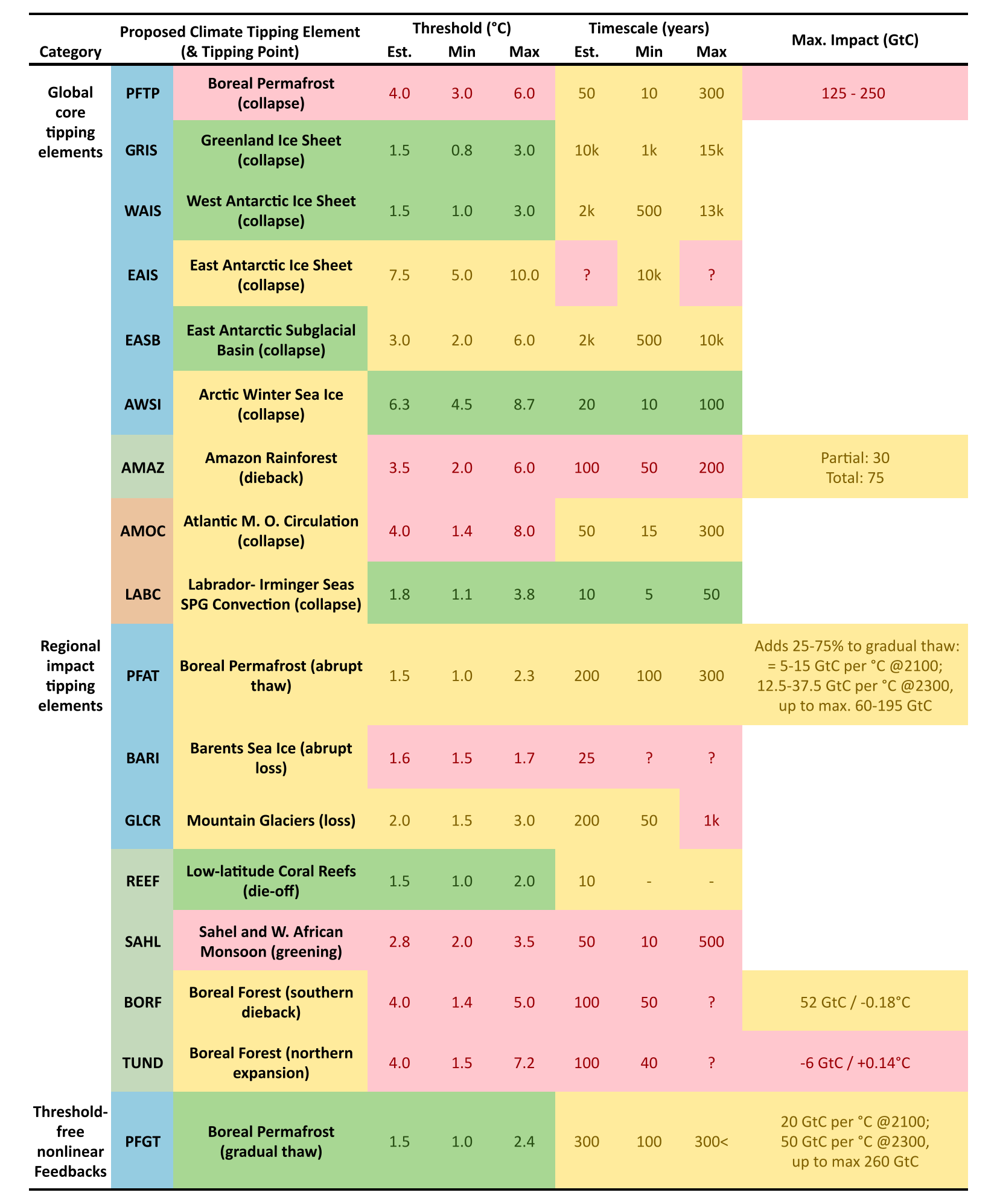
In their recent literature synthesis, Armstrong McKay et al. (2022) identify 16 TEs within the Earth system and provide estimates of their threshold temperatures, the characteristic timescales their tipping is assumed to unfold over and their impact on global warming (Table 1 – we will use the abbreviations defined in the table for the different TEs). Building on the definition of TEs by Lenton et al. (2008), Armstrong McKay et al. (2022) distinguish between “global core” and “regional impact” TEs. To qualify as a global core TE, a tipping point has to occur uniformly across a sub-continental scale (∼ 1000 km) for a subsystem of the Earth. However, if the change in forcing is approximately uniform across a large spatial area, small-scale tipping points can be crossed near-synchronously at a sub-continental scale, which qualifies the affected subsystem as a regional impact TE. Furthermore, in their intact (not tipped) state, global TEs have to contribute significantly to the overall operation mode of the Earth system, while regional impact TEs are required either to contribute significantly to human welfare or to have great value in themselves as unique features of the Earth system.

Since the triggering of TEs will negatively affect human welfare, political efforts should be increased to avoid them (Cai et al., 2016). However, it is not straightforward to determine how safe a specific emission scenario is with regard to triggering TEs, since several uncertainties need to be accounted for within this calculation. The climate sensitivity to anthropogenic emissions remains poorly constrained, with a likely range of the equilibrium climate sensitivity to a doubling of atmospheric CO₂ concentrations of 2.5–4 °C (Chen et al., 2021). Furthermore, climate tipping points include uncertainties within their threshold temperatures, timescales and impacts, and for some even their existence remains uncertain (Armstrong McKay et al., 2022). Additional uncertainty is introduced by potential interactions of climate tipping points, which tend to destabilise them (Wunderling et al., 2021). Such interactions can be of manifold nature and often involve complex mechanisms. One example are TEs within the Earth's carbon cycle, which have the potential to release large amounts of greenhouse gases (GHGs) and thereby amplify global warming, which in turn increases the probability of triggering other TEs (Steffen et al., 2018).

In this study, we calculate probabilities of triggering for the 16 TEs that Armstrong McKay et al. (2022) identify within the Earth system, including the uncertainties in climate sensitivities and the threshold temperatures, by employing a Monte Carlo approach (Metropolis et al., 1953). Herewith, we provide an update of the widely used but somewhat outdated probabilities of triggering derived from an expert elicitation conducted by Kriegler et al. (2009). Furthermore, we quantify the additional warming that might arise from TEs within the Earth's carbon cycle and how it increases the probabilities of triggering other TEs.

TEs with the potential to significantly impact the Earth's carbon cycle include abrupt permafrost thaw or collapse, Amazon rainforest dieback, and the northern expansion and the southern dieback of boreal forest (Armstrong McKay et al., 2022). Since northern expansion and southern dieback of boreal forests balance out in terms of global warming, we exclude them from our analysis. The exact nature of this balance remains contested. The latest IPCC report assumes that the expansion of boreal forests at their northern edge and dieback of boreal forests accompanied by temperate forest invasion at the southern edge of boreal forests will roughly balance out in terms of carbon emissions (Canadell et al., 2021). On the other hand, Armstrong McKay et al. (2022) argue that the carbon release from southern dieback will be an order of magnitude larger than the sequestered carbon from the northern expansion of boreal forests, but the warming would still balance out since it is to first order determined by albedo and evapotranspiration changes (Table 1). Permafrost thaw can be further subdivided into three distinct processes: gradual permafrost thaw, which is a threshold-free feedback to global warming; abrupt permafrost thaw, which is a regional impact tipping element; and permafrost collapse, which is a global core tipping element (Armstrong McKay et al., 2022). Since the gradual thaw of permafrost, associated with uniform and large-scale deepening of the active layer, is not assumed to include a tipping point, we do not include it in our analysis (Nitzbon et al., 2024). Instead, we focus on abrupt thaw and collapse of permafrost and Amazon dieback, hereafter referred to as the “carbon tipping elements”.

The abrupt thaw of permafrost occurs regionally but near-synchronously over the permafrost region due to thermokarsts which can affect several metres of permafrost within days to weeks (Turetsky et al., 2019). The emerging landscapes mostly include water-saturated soils (Olefeldt et al., 2016); hence high methane emissions from anaerobic respiration of the now accessible soil organic carbon must be expected. Around 20 % of the carbon emissions from abrupt permafrost thaw are assumed to be released as methane (Turetsky et al., 2020). Abrupt permafrost thaw is assumed to amplify gradual thaw, since they spread at similar rates in dedicated permafrost models (Turetsky et al., 2020; Armstrong McKay et al., 2022). The collapse of permafrost can be caused by permafrost degradation becoming self-perpetuating due to the heat released by microbial respiration of soil organic carbon, leading to further thaw of permafrost and resulting in a positive feedback loop, which is referred to as the “compost bomb instability” (Luke and Cox, 2011; Khvorostyanov et al., 2008). This process might occur in the Yedoma region or in abruptly dried permafrost soils (Armstrong McKay et al., 2022). Abrupt dieback of the Amazon is assumed to occur due to reduced moisture recycling and forest-fire feedbacks triggered by initial tree loss due to either global warming or deforestation, whereby only the former is accounted for in this study (Science Panel for the Amazon, 2021; Nobre et al., 2016; Flores et al., 2024). We follow Armstrong McKay et al. (2022) by defining carbon emissions from Amazon dieback as the carbon that would be released from the forest itself, which does not include an increase in atmospheric carbon due to a diminished capability of the Amazon to act as a carbon sink in the case of dieback.

It has recently been shown by Ritchie et al. (2021) that threshold temperatures can be temporarily exceeded without triggering the TE if the overshoot time is small compared to the effective timescale of the TE. It is possible to include this effect in a conceptual representation of tipping processes, based on the internal timescales of TEs from Armstrong McKay et al. (2022), like that demonstrated for a subset of TEs by Wunderling et al. (2023). While the internal timescale of a TE is defined as the time it takes the TE to tip from one stable state to the other, the effective timescale is a measure of the recovery time from perturbations in the initial stable state. Since the connection between the two does not seem straightforward to us and the internal timescales of at least 4 of the 16 TEs discussed in this study remain unconstrained (Table 1), we think it is not yet possible to make precise statements about the timing of triggering TEs. Instead, we adopt the most simple case for which the effective timescales are zero, i.e. a TE is triggered instantaneously once its threshold temperature is crossed. To show that this approach would lead to an overestimation of probabilities of triggering for emission scenarios producing a temperature overshoot, we also discuss the case of equilibrium triggering. Here, we assume that the effective timescales of the TEs are long compared to the overshoot time; i.e. a TE is only triggered if the stabilised temperature at the end of the model period exceeds the threshold temperature. The real probability of triggering will be somewhere between the probability of instantaneous triggering and the probability of equilibrium triggering, but it remains unknown.

To analyse how carbon TEs and our assumption about the effective timescale of TEs affect the probabilities of triggering, we derive three estimates of the probability of triggering with different degrees of conservatism: equilibrium triggering, instantaneous triggering and instantaneous triggering including the effect of carbon TEs. Distinguishing between the probabilities of instantaneous and equilibrium triggering allows us to estimate the magnitude of the uncertainty in the triggering probability resulting from not knowing the effective timescale of the TEs. The probability of instantaneous triggering can be interpreted as an upper bound and the probability of equilibrium triggering as a lower bound on the probability of triggering if interactions between TEs are ignored. The third probability estimate allows us to investigate how much the upper bound of the triggering probabilities could be increased by carbon TEs.

Our model framework relies on the second version of the Finite amplitude Impulse Response model (FaIRv2.0.0), a 0D reduced complexity climate model developed by Leach et al. (2021), and the estimates for the threshold temperatures, timescales and impacts of TEs from Armstrong McKay et al. (2022). These estimates are used to build a conceptual carbon tipping elements model (CTEM), which can be coupled to FaIR to include the additional carbon emissions from carbon TEs. With this setup, we generate a “coupled” (CTEM coupled to FaIR) and an “uncoupled” (FaIR only) large-scale model ensemble for five Shared Socioeconomic Pathways (SSPs) (O'Neill et al., 2016). Hereby, we propagate the involved uncertainties up until the year 2500. To assess the risk of current policies for triggering climate tipping points, we focus our analysis on SSP2-4.5. With a median warming of 2.8 °C in 2100 produced by FaIR, this scenario is closest to the estimated warming in 2100 resulting from current policies (2.7 °C – Climate Action Tracker, 2022; 2.8 °C – United Nations Environment Programme, 2022; 2.6 °C – Meinshausen et al., 2022).

Our approach is explained in more detail in the next section. In Sect. 3 we investigate the carbon emissions and in Sect. 4 the additional warming from carbon TEs, followed by a presentation of the probabilities of triggering TEs in Sect. 5. We discuss our results in Sect. 6 and conclude with Sect. 7.

Table 1 Category, threshold, timescale and impact of the TEs, reproduced from Armstrong McKay et al. (2022). Colours of the second column on the left represent the Earth system domain of the tipping point (blue: cryosphere; green: biosphere; orange: ocean/atmosphere). All other colours represent confidence, with green being high confidence, yellow medium confidence and red low confidence.

2 Data and methods

2.1 SSP emission pathways

We use the CMIP6 GHG and aerosol emissions and effective radiative forcing datasets employed in the Reduced Complexity Model Intercomparison Project (Nicholls et al., 2020). Both datasets contain global average values with an annual time step throughout the historical period (1750–2014) which shifts to a decadal time step for the projection period (2015–2500).

The CMIP6 GHG and aerosol emission projections for the five different SSP scenarios follow Gidden et al. (2019). The emission extensions beyond 2100 follow the conventions described in Meinshausen et al. (2020). Historical emissions (1750–2014) of chemically reactive gases (CO, CH₄, NH₃, NO_x, SO₂, non-methane volatile organic compounds), carbonaceous aerosols (black carbon and organic carbon) and CO₂ come from the Community Emissions Data System (Hoesly et al., 2018). Historical biomass burning emissions of CH₄, black carbon, CO, NH₃, NO_x, organic carbon, SO₂ and non-methane volatile organic compounds come from Van Marle et al. (2017). Global historical CO₂ emissions from land use are taken from the Global Carbon Budget 2016 (Le Quéré et al., 2016). The regional breakdown of land-use CO₂ emissions and N₂O emissions comes from the Potsdam Real-Time Integrated Model for probabilistic Assessment of emissions Paths for historical emissions version 1.0 (Guetschow et al., 2016). Data gaps in the historical emissions were filled with inverse emissions based on CMIP6 concentrations from the Model for the Assessment of Greenhouse Gas Induced Climate Change (MAGICC) 7.0.0 (Meinshausen et al., 2020).

Effective radiative forcing from changes in land use, solar insulation and volcanic activity used within FaIR follows the data provided by Smith (2020).

2.2 The FaIR model

To map GHG and aerosol emissions to GMST, including the uncertainty in equilibrium climate sensitivities (ECSs), we use the FaIRv2.0.0 model developed by Leach et al. (2021), which is run with an annual time step. It consists of six equations, five of which are adopted from Myhre et al. (2013). The sixth equation implements a state dependency of the carbon cycle, which enables a better representation of the relationship between emissions and atmospheric concentrations for historical observations and projections (Leach et al., 2021). Despite its relative simplicity, FaIR is flexible enough to emulate more complex Earth system models (ESMs) from CMIP6. FaIR allows for probabilistic projections of GMST by relying on a parameter ensemble informed by CMIP6 models and constrained with the observed trend and level of global warming. However, the parameterisation of FaIRv2.0.0 developed by Leach et al. (2021) is not constrained enough to rule out potentially unrealistically high ECSs with a 95th percentile of 6.59 °C compared to 5 °C reported by Forster et al. (2021). Since we rely on this constrained parameter ensemble to include the uncertainty in ECSs in our predictions of GMST, extremely high temperatures towards the end of the model period might be unrealistic.

2.3 Carbon tipping elements model

We introduce the simple, system-dynamics-type model CTEM to investigate the carbon emissions that might arise from the tipping of AMAZ, PFTP and PFAT and the respective warming caused by them, which, in turn, increases the probabilities of triggering other TEs. CTEM is able to represent the carbon emissions from AMAZ, PFAT and PFTP, with threshold temperatures, timescales and impacts consistent with the estimates from Armstrong McKay et al. (2022) (Table 1). Each TE is represented by the stock of cumulative carbon emissions it adds to the SSP carbon emissions. The cumulative emissions are represented by the following logistic equation:

$$\begin{array}{}\text{(1)}& {\displaystyle \frac{\mathrm{d}S}{\mathrm{d}t}}=r\left({\displaystyle \frac{T}{Q}}\right)S\left(\mathrm{1}-{\displaystyle \frac{S}{K}}\right),\end{array}$$

with S being cumulative carbon emissions (in Gt C), r the maximum growth rate (in yr⁻¹), K the maximum impact (in Gt C), Q the threshold temperature (in °C), T the GMST relative to pre-industrial levels (in °C) and t the time (in years). The rate dependence of all three TEs found by Armstrong McKay et al. (2022) is included with the term $T/P$, which means a higher exceedance of the threshold temperature causes faster change in S. Once T exceeds Q, the carbon TE will be triggered; i.e. we assume the case of instantaneous triggering.

For AMAZ and PFTP, the impact is independent of GMST once they are triggered (Table 1). Therefore, Eq. (1) can be used to represent them without further modifications being necessary. PFAT, however, is assumed to amplify PFGT, which is a threshold-free feedback. Therefore, the impact of PFAT also depends on GMST, with higher temperatures leading to increased carbon emissions, as well as different values for this feedback in 2100 and 2300 (Table 1). Hence, for PFAT K from Eq. (1) needs to be calculated as

$$\begin{array}{}\text{(2)}& K=min(F\cdot T,K_{\max }),\end{array}$$

with

$$\begin{array}{}\text{(3)}& F=\left\{\begin{array}{l}{F}_{\mathrm{100}}\forall t\le \mathrm{2100},\\ F_{\mathrm{100}}\cdot \frac{\mathrm{2300}-t}{\mathrm{200}}+F_{\mathrm{300}}\cdot \frac{t-\mathrm{2100}}{\mathrm{200}}\forall \mathrm{2100}<t<\mathrm{2300},\\ F_{\mathrm{300}}\forall t\ge \mathrm{2300}.\end{array}\right.\end{array}$$

Here, K is calculated as the product of the feedback strength F (in Gt C °C⁻¹) and GMST (in °C), limited to the maximum impact K_max (in Gt C) of PFAT. In Eq. (3), we define F as the feedback strength for the year 2100 (F₁₀₀) before and in 2100 and as the feedback strength for the year 2300 (F₃₀₀) in and after 2300, and we interpolate linearly between these two values between 2100 and 2300.

The resulting set of three differential equations (one for each TE) is solved using a forward difference scheme, similar to the implementation of FaIR (supplement of Leach et al., 2021). In FaIR, output variables such as T are assumed to be average values between two consecutive time steps (denoted by a bar over t), while the values for the input variables such as the annual SSP GHG emissions (E_SSP) reside at each time step (no bar over t). To be consistent with this implementation, we define S and the resulting annual carbon emissions from each TE (E_TE) also at each time step (Fig. S1). To calculate S for each time step (t) with a step size (Δt) of 1 year, we integrate Eq. (1), which yields

$$\begin{array}{}\text{(4)}& S\left(t\right)={\left(e^{-a\left(\stackrel{\mathrm{‾}}{t-\mathrm{1}}\right)\mathrm{\Delta }t}\left(S^{-\mathrm{1}}(t-\mathrm{1})-{\displaystyle \frac{b\left(\stackrel{\mathrm{‾}}{t-\mathrm{1}}\right)}{a\left(\stackrel{\mathrm{‾}}{t-\mathrm{1}}\right)}}\right)+{\displaystyle \frac{b\left(\stackrel{\mathrm{‾}}{t-\mathrm{1}}\right)}{a\left(\stackrel{\mathrm{‾}}{t-\mathrm{1}}\right)}}\right)}^{-\mathrm{1}},\end{array}$$

with the auxiliary variables a and b being calculated as

$$\begin{array}{c}{\displaystyle }a\left(\stackrel{\mathrm{‾}}{t-\mathrm{1}}\right)=r{\displaystyle \frac{T\left(\stackrel{\mathrm{‾}}{t-\mathrm{1}}\right)}{P}},\\ {\displaystyle }b\left(\stackrel{\mathrm{‾}}{t-\mathrm{1}}\right)={\displaystyle \frac{rT\left(\stackrel{\mathrm{‾}}{t-\mathrm{1}}\right)}{PK}}.\end{array}$$

For PFTP and AMAZ Eq. (4) can be used directly to calculate S, but for PFAT K needs to be calculated using Eq. (2) with $T=T\left(\stackrel{\mathrm{‾}}{t-\mathrm{1}}\right)$ and is therefore also time-dependent (for the full derivation please see Sect. S2). The irreversibility of carbon emissions from all three TEs is implemented by setting negative changes of S to zero.

CTEM needs to be calibrated to match the estimated behaviour summarised in Table 1. While values for F₁₀₀, F₃₀₀, K, K_max and Q can be used in CTEM directly, r and the initial stock (S₀) need to be calibrated or defined for the model to match the proposed tipping timescales (H). For this purpose, we define the H as the period over which 99 % of the cumulative emissions occur. While H and the corresponding value of r are calibrated for the whole range of H given in Table 1 for PFTP and AMAZ, PFAT is implemented slightly differently since K depends on T (Eq. 2). For PFAT, H is included implicitly in the feedback parameters F₁₀₀ and F₃₀₀, with high values corresponding to short H and vice versa. Therefore, we keep H and the corresponding r fixed at their mean value for PFAT, with varying values for the feedback parameters. In the calibrated version of CTEM, the evolution of S follows the characteristic “S” shape of logistic equations (Fig. 1). Further information on the calibration of CTEM is given in Sect. S3. A test of the calibration shows that the timescales produced by CTEM are generally matching the expected behaviour for AMAZ and PFTP (Fig. S3) but not for PFAT (Fig. S4). For PFAT we find that the carbon emissions are generally too low in 2100; however, this emission deficit is removed until 2300, when emissions of PFAT match the estimates. We regard this deviation to be acceptable given the simplicity of our model approach (see Sect. S4 for further information).

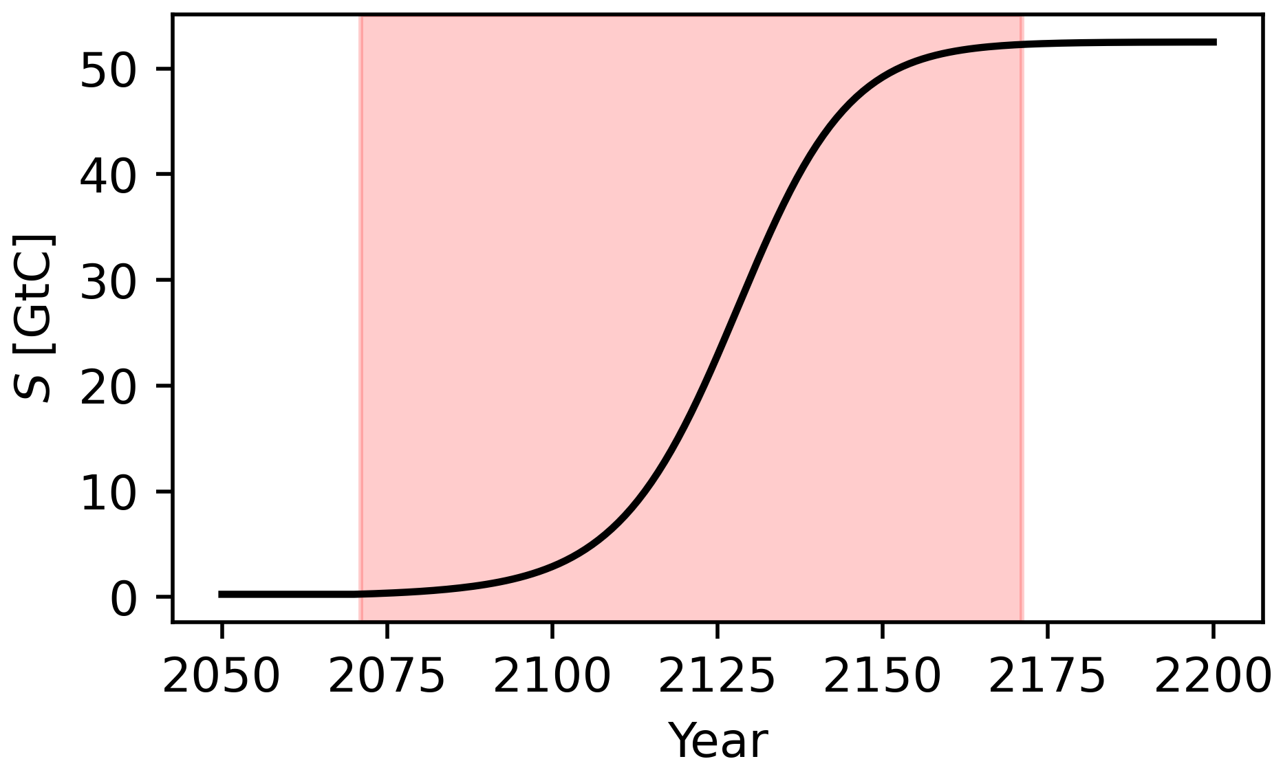
Figure 1 S for the calibration of the mean timescale of AMAZ (under SSP5-8.5). The red shaded area denotes the period over which 99 % of the cumulative carbon emissions occur.

Coupling to FaIR

CTEM is coupled to FaIR every time step by adding E_TE to E_SSP. For each TE, we calculate E_TE from S as

$$E_{\mathrm{TE}}\left(t\right)=S\left(t\right)-S(t-\mathrm{1}).$$

The total carbon emissions E_TE are split up into CO₂ and CH₄ emissions for all three TEs. For PFAT, we assume that 20 % of the carbon is emitted as CH₄, following Turetsky et al. (2020), while no CH₄ emissions are expected from AMAZ (Armstrong McKay et al., 2022). Quantifying the fraction of CH₄ emissions arising from PFTP is challenging due to the lack of previous model studies and limited process understanding. We rely on the 2D model study conducted by Schneider von Deimling et al. (2015), who report 40 % of additional warming due to CH₄ emissions from the Yedoma deposits, which can be associated with PFTP. Since this amplification is within the uncertainty range of additional warming caused by CH₄ emissions from gradual permafrost thaw of 35 %–48 % for which 2.3 % of the carbon is emitted as methane (Schuur et al., 2015), we assume that this fraction of CH₄ emissions also holds for PFTP. The annual CH₄ and CO₂ emissions of all three TEs are then added to the E_SSP(t) of the respective SSP, and the sum is used to run the next time step of FaIR, calculating $T\left(\stackrel{\mathrm{‾}}{t}\right)$ which is then used to force CTEM and so on.

To avoid the double-counting of carbon emissions, carbon emissions from the carbon TEs modelled by CTEM must not be included in FaIR. We can rule this possibility out, since carbon emissions from carbon TEs are neither accounted for by the CMIP6 models used to parameterise FaIR nor of major importance for the observed warming signal used to constrain the parameter ensemble (see Sect. S6 for further explanation and references).

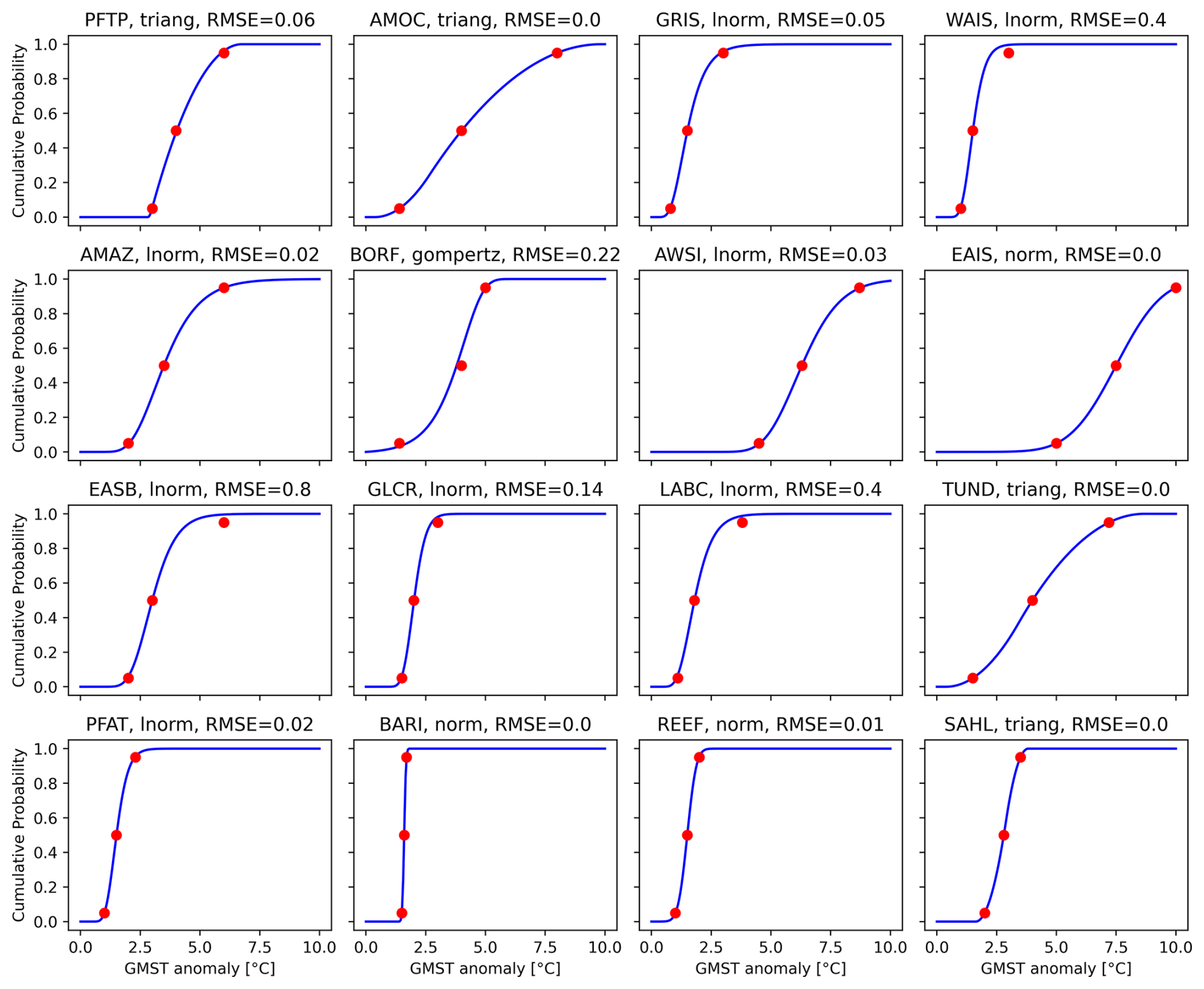
Figure 2 Cumulative distribution functions of Q for all TEs, together with the RMSE between the given percentiles (red dots) and the actual percentiles of the respective distribution. The title states TE, distribution type and RMSE in °C.

2.4 Generation of model ensembles

We construct a coupled (FaIR coupled to CTEM) and an uncoupled (FaIR only) 5000-member model ensemble for SSP1-1.9, SSP1-2.6, SSP2-4.5, SSP3-7.0 and SSP5-8.5. Hereby, we follow a Monte Carlo scheme (Metropolis et al., 1953) to propagate the uncertainties within FaIR and CTEM.

For the parameterisation of FaIR, we randomly select 5000 members of its constrained parameter ensemble. We use the same parameter sample for FaIR in both the coupled and the uncoupled ensemble to make sure that changes in the climate response only arise from carbon emissions of the carbon TEs.

For the parameterisation of CTEM and the calculation of triggering probabilities, we construct probability distributions of the respective parameters based on the estimates given in Table 1. From those probability distributions, we sample parameter values, employing Latin hypercube sampling (McKay et al., 1979).

To calculate the probability of triggering, we sample the uncertainty range of Q for all TEs, again using the same parameter sample for both ensembles. For the sampling process of Q, we infer probability distributions from the estimates in Table 1, deciding that the minimum estimate, the best estimate and the maximum estimate should correspond to the 5th, the 50th and the 95th percentile of the respective probability distribution. To determine the probability distributions which best fit those percentiles, we use the “rriskDistributions” package (Belgorodski et al., 2017), which chooses from 17 continuous probability distributions, minimising the absolute difference between the given and the actual percentiles. We derive eight log-normal, four triangular, three normal and one Gompertz distribution (Fig. 2). While some distributions of Q agree perfectly with the given percentiles (AMOC, EAIS, TUND, BARI, SAHL), others deviate substantially with RMSEs higher than 0.2 °C (WAIS, BORF, EASB, LABC). In the case of WAIS, EASB and LABC, this deviation is mainly caused by values that are too low at the 95th percentile, which is reached at 2.3 °C rather than 3 °C for WAIS, 4.6 °C rather than 6 °C for EASB and 3.1 °C rather than 3.8 °C for LABC. In the case of BORF, the relatively high RMSE is caused by a value that is too high at the 5th percentile (1.7 °C rather than 1.4 °C) and a value that is too low at the 50th percentile (3.8 °C rather than 4 °C), while the 95th percentile agrees well with the expected value (less than 0.02 °C deviation). Even though the deviations between the given and the actual percentiles of those four TEs are significant, we regard them to be acceptable, since the given percentiles of Q from Armstrong McKay et al. (2022) also remain somewhat speculative. Nevertheless, it must be kept in mind that high probabilities of tipping might be reached at values of GMST that are too low for WAIS, EASB and LABC due to their imperfect probability distributions of Q.

We now turn to the parameterisation of CTEM. For the distribution of H for PFTP and AMAZ, we derive one log-normal distribution each, following the same approach as for the generation of probability distributions of Q (Fig. S5). The impacts K of PFTP and AMAZ and the maximum impact K_max of PFAT are sampled from continuous uniform distributions, with the same probability for all values within the given ranges from Table 1 (Fig. S6). We regard this reasonable since Armstrong McKay et al. (2022) only give maximum and minimum values for those variables, and we do not have any additional information about their distribution. The feedback strengths F₁₀₀ and F₃₀₀ of PFAT are also sampled from continuous uniform distributions, with the same probability for all values within the given ranges from Table 1 (Fig. S7). Here, the same argument holds as for the selection of the distributions of K and K_max.

We assume that all parameters within the parameter set of CTEM are uncorrelated except for F₁₀₀ and F₃₀₀, which are correlated with a correlation coefficient of 1. The decision about the correlation of the parameters represents our understanding that there are no correlations, or at least no clear evidence for them, between the threshold temperatures, the timescales or the impacts of AMAZ, PFAT and PFTP. The correlation between F₁₀₀ and F₃₀₀ is established since H of PFAT is included in those parameters, and we assume that H is constant over time; e.g. a low feedback in 2100 associated with a high H also means low feedback in 2300 due to the same high H that the emissions occur over.

2.5 Calculation of tipping probabilities

To calculate the probabilities of triggering any of the 16 TEs discussed in this study, we sample one value of Q from the respective distribution (Fig. 2) for each TE and each ensemble member. For both ensembles, we calculate the probability of instantaneous triggering by counting a TE as triggered once T of an ensemble member exceeds Q. Since all TEs discussed here are by definition irreversible on the considered timescale, the share of triggered TEs cannot decrease with time, even if T would decrease. For the uncoupled ensemble, we calculate the probability of equilibrium triggering by checking for each ensemble member if the average T between 2400 and 2500 exceeds Q. Probabilities of triggering are defined as the ratio between ensemble members for which the TE is triggered and the total ensemble members.

2.6 Robustness of the results

To examine whether an ensemble of size 5000 is sufficiently large to approximate the distributions of the output variables with our Monte Carlo approach, we create 20 coupled ensembles with 5000 members and run under SSP5-8.5, sampling uncertainties within FaIR and CTEM. As carbon emissions from CTEM are used to calculate T, which is also the final output variable of FaIR, it includes uncertainties from all parameters and is hence expected to vary most between different ensembles. Therefore, we inspect the deviation of T between the 20 ensembles. While the 5th percentile and the mean of T are nearly equal for all ensembles, with standard deviations below 0.06 °C at all times, the 95th percentile deviates slightly between the ensembles, with a standard deviation of up to 0.24 °C (Fig. S8). Given the range of T between the 5th and the 95th percentile of ∼11 °C, we regard those deviations to be sufficiently small.

3 Carbon emissions from carbon tipping elements

The carbon emissions from carbon TEs increase from SSP1-1.9 to SSP5-8.5 (Fig. 3, Table 2). While zero carbon emissions from carbon TEs remain possible under SSP1-1.9 and SSP1-2.6, high carbon emissions become much more likely under SSP2-4.5, with the maximum emissions being nearly as high as under SSP5-8.5. This is a direct consequence of the probabilities of instantaneous triggering of carbon TEs. Under SSP1-2.6, the triggering of PFAT occurs for 79 % of the ensemble members, while the triggering of AMAZ and PFTP only happens for 13 % and 5 % respectively. Under SSP2-4.5, triggering probabilities are increased substantially to 98 % for PFAT, 53 % for AMAZ and 37 % for PFTP. This means that maximum carbon emissions with all three carbon TEs triggered become more likely under SSP2-4.5 compared to SSP1-2.6.

Even though the highest carbon emissions from carbon TEs occur under SSP3-7.0 and SSP5-8.5, they remain small compared to anthropogenic carbon emissions (Fig. 3). The 95th percentile of cumulative carbon emissions from carbon TEs only reaches 14 % of the cumulative anthropogenic carbon emissions in 2500 under SSP3-7.0 and 10 % under SSP5-8.5. The relative contribution of carbon emissions from carbon TEs to the total carbon emissions increases towards lower-emission scenarios. Under SSP2-4.5 the 95th percentile of cumulative carbon emissions from carbon TEs reaches 35 % of the cumulative anthropogenic carbon emissions in 2500, 40 % under SSP1-2.6 and 84 % under SSP1-1.9.

Hence, SSP2-4.5 is special in the sense that maximum carbon emissions from carbon TEs are already possible and are large relative to the anthropogenic emissions.

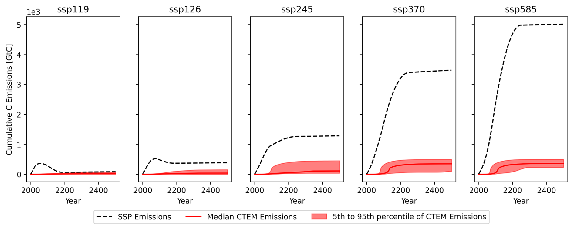
Figure 3 Cumulative carbon emissions from all SSP scenarios and the carbon TEs (modelled by CTEM) between 2000 and 2500.

Table 2 Median and 5th–95th percentile range of cumulative CO₂ and CH₄ emissions from the carbon TEs and the GMST increase (dT) caused by them. All quantities are calculated individually for each ensemble member as the increase caused by carbon TEs compared to the respective uncoupled ensemble member.

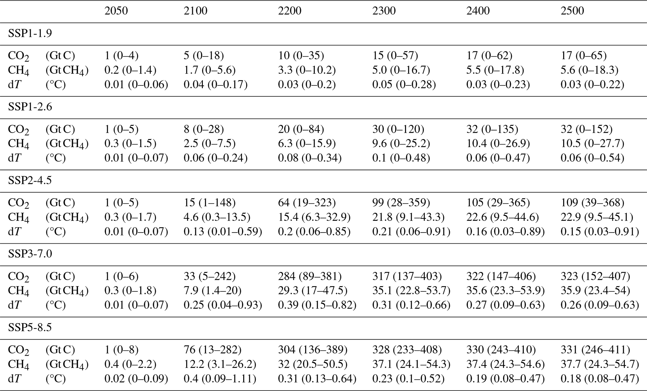
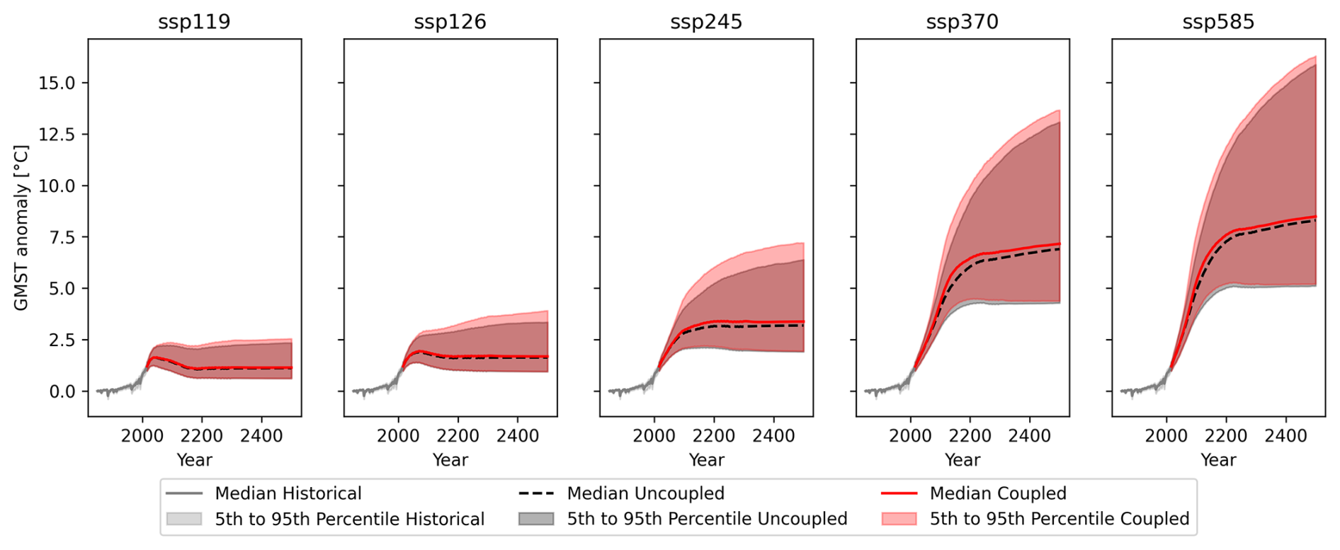
Figure 4 GMST relative to the 1850–1900 period of the coupled and the uncoupled ensemble, together with the historical evolution.

4 Increase in global warming caused by carbon tipping elements

The carbon emissions from carbon TEs cause an increase in global warming (Fig. 4). Under SSP1-1.9 and SSP1-2.6, high temperature increases from carbon TEs are possible but not common, with the temperature distributions skewed towards higher values. No additional warming from carbon TEs remains possible under both scenarios, with the 5th percentile being zero at all times (Table 2). Under SSP2-4.5, high impacts from carbon TEs become more common compared to SSP1-2.6. This is indicated by the median temperature increase, which reaches its maximum of 0.22 °C in 2300 under SSP2-4.5, compared to only 0.08 °C being reached in the same year under SSP1-2.6 (Table 2). Additional warming from carbon TEs becomes the default case under the high-emission scenarios SSP3-7.0 and SSP5-8.5. The 5th percentile of the temperature increase is well above zero after 2100 for both scenarios, and the median reaches 0.39 and 0.4 °C in 2300 and 2200 under SSP3-7.0 and SSP5-8.5 respectively (Table 2).

High additional warming from carbon TEs mostly occurs for ensemble members with a high climate sensitivity. This is indicated by the 95th percentile of the temperature distribution increasing more than all other percentiles if the warming from carbon TEs is included (Fig. 4). This effect is especially pronounced under SSP1-2.6 and SSP2-4.5.

It is interesting to see that the highest long-term temperature increase from carbon TEs becomes possible under SSP2-4.5, with the 95th percentile reaching 0.91 °C in 2500, and not under scenarios with higher anthropogenic emissions (Table 2). This is in contradiction to the cumulative CO₂ and CH₄ emissions from carbon TEs, which are higher under high-emission scenarios than under SSP2-4.5. The reason for this behaviour is the implementation of the forcing relationship translating atmospheric CO₂ and CH₄ concentrations to radiative forcing developed by Etminan et al. (2016) and used in FaIR. It is approximated by a logarithmic and a square-root term for CO₂ and by a square-root term for CH₄, meaning that the effect of additional atmospheric concentrations of both GHGs on GMST is decreasing for higher atmospheric concentration levels. Therefore, the amount of carbon emissions from carbon TEs relative to the anthropogenic emissions is decisive to determine the additional warming from carbon TEs.

Nevertheless, it must be noted that the highest short-term temperature increase from carbon TEs becomes possible under the high-emission scenarios SSP3-7.0 and SSP5-8.5, with the 95th percentile reaching 0.93 and 1.11 °C in 2100 under SSP3-7.0 and SSP5-8.5 respectively. This can be linked to high CH₄ emissions from fast PFAT degradation due to rapidly increasing temperatures, which leads to peaks in the atmospheric CH₄ concentration anomaly around 2100 (Fig. S9).

The temperature increase from carbon TEs occurs earlier under high-emission scenarios (Table 2), which can be explained by threshold temperatures of the carbon TEs being crossed earlier under those scenarios, as the general temperature increase is faster (Fig. 4). Interestingly, the median temperature increase from carbon TEs is declining towards the end of the model period under all SSPs (Table 2). This can be linked to the decreasing atmospheric methane concentrations (Fig. S9).

When comparing the different SSPs, it becomes evident that high temperature increases from carbon TEs are possible but rare under low-emission scenarios, and they become more frequent but less strong compared to the anthropogenic warming under high-emission scenarios (Table 2 and Fig. 4). This means that if anthropogenic carbon emissions can be limited to levels comparable to SSP1-2.6, there remains a risk that the warming might be substantially increased by triggering carbon TEs. On the other hand, if anthropogenic emissions keep increasing like under SSP5-8.5, warming will almost certainly be amplified by carbon TEs; however, this additional warming will remain small compared to the anthropogenic warming. On average, the additional warming from carbon TEs is low compared to the anthropogenic warming and the risk for high temperature increases is limited. This is indicated by the median temperature increase from carbon TEs always remaining at least 1 order of magnitude smaller than the median anthropogenic warming (Table 2 and Fig. 4).

Table 3 Probability (P) of triggering averaged over all TEs for the case of equilibrium triggering, instantaneous triggering and instantaneous triggering including the additional warming from carbon TEs.

5 Probabilities of triggering climate tipping elements

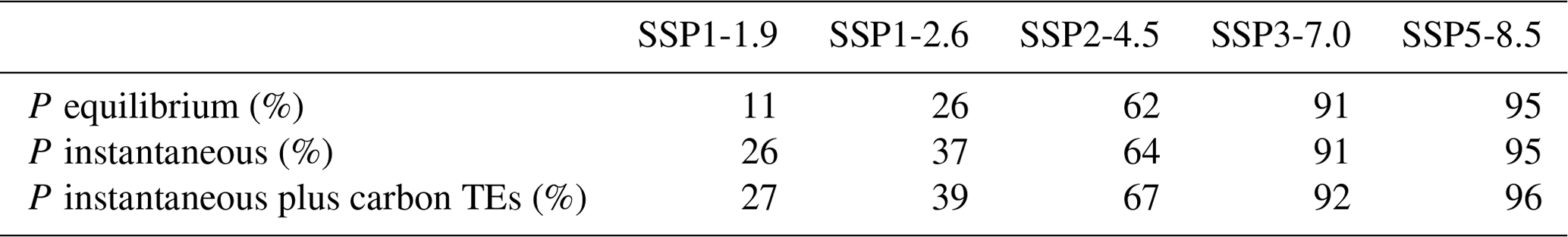
We now turn to the probabilities of triggering any of the 16 TEs proposed by Armstrong McKay et al. (2022) (Table 1) under the five SSPs and how those probabilities are increased by the additional warming from carbon TEs. We distinguish between three probability estimates: the probability of equilibrium triggering, the probability of instantaneous triggering and the probability of instantaneous triggering including the additional warming from carbon TEs. Probabilities of triggering generally increase in this order (Table 3). The increase in probability from the case of equilibrium triggering to the case of instantaneous triggering is due to our assumptions about the effective timescale of TEs, assuming a long effective timescale compared to the temperature overshoot times, or an effective timescale of zero. The additional increase in probability of triggering from carbon TEs becomes visible when comparing the probabilities of instantaneous triggering with and without including the effect of carbon TEs.

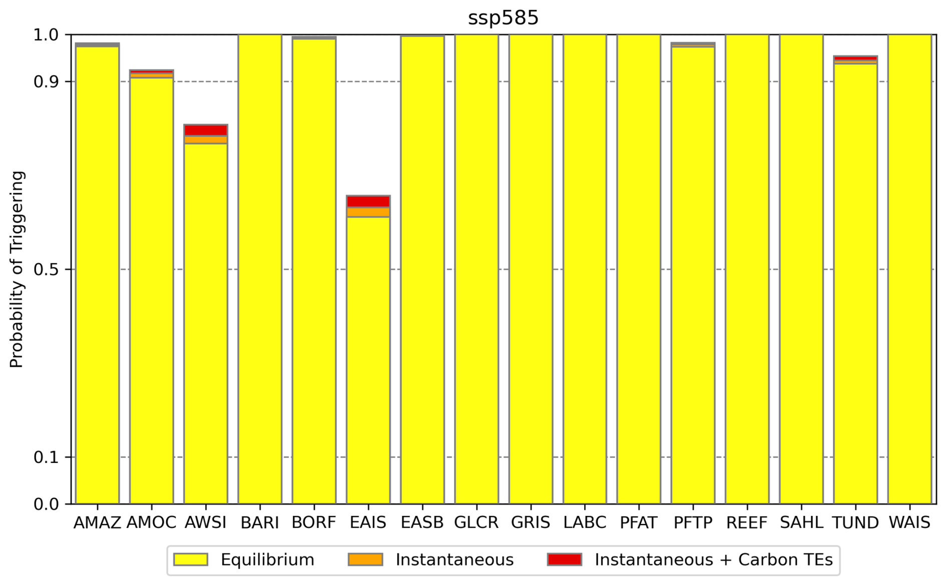
Figure 5 Probabilities of triggering the TEs under SSP5-8.5 for the case of equilibrium triggering, instantaneous triggering and instantaneous triggering including the additional warming from carbon TEs.

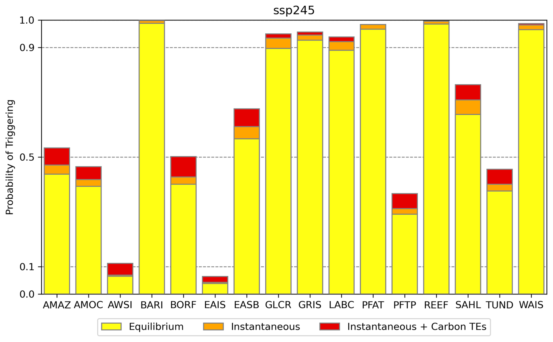
Figure 6 Probabilities of triggering the TEs under SSP2-4.5 for the case of equilibrium triggering, instantaneous triggering and instantaneous triggering including the additional warming from carbon TEs.

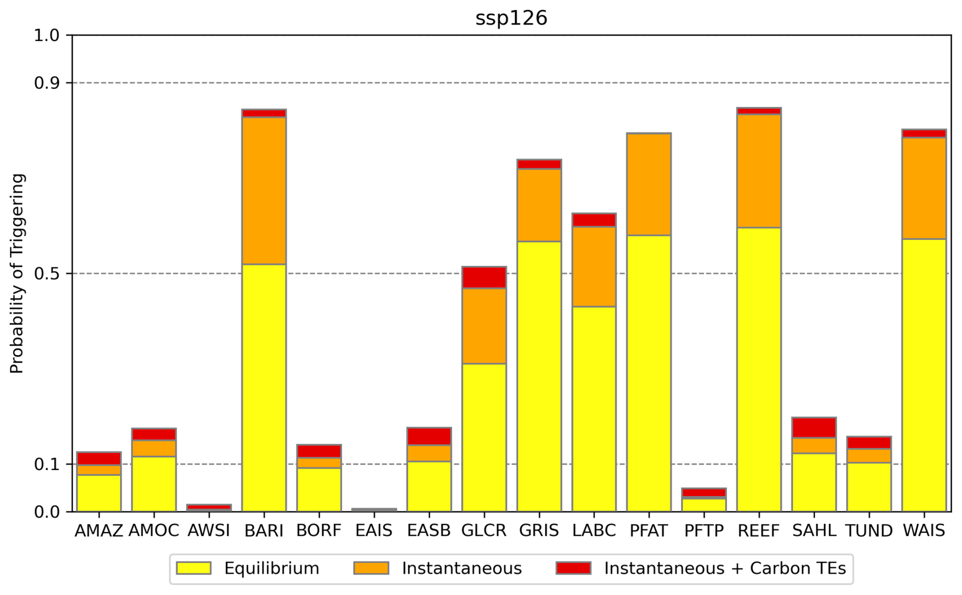
Figure 7 Probabilities of triggering the TEs under SSP1-2.6 for the case of equilibrium triggering, instantaneous triggering and instantaneous triggering including the additional warming from carbon TEs.

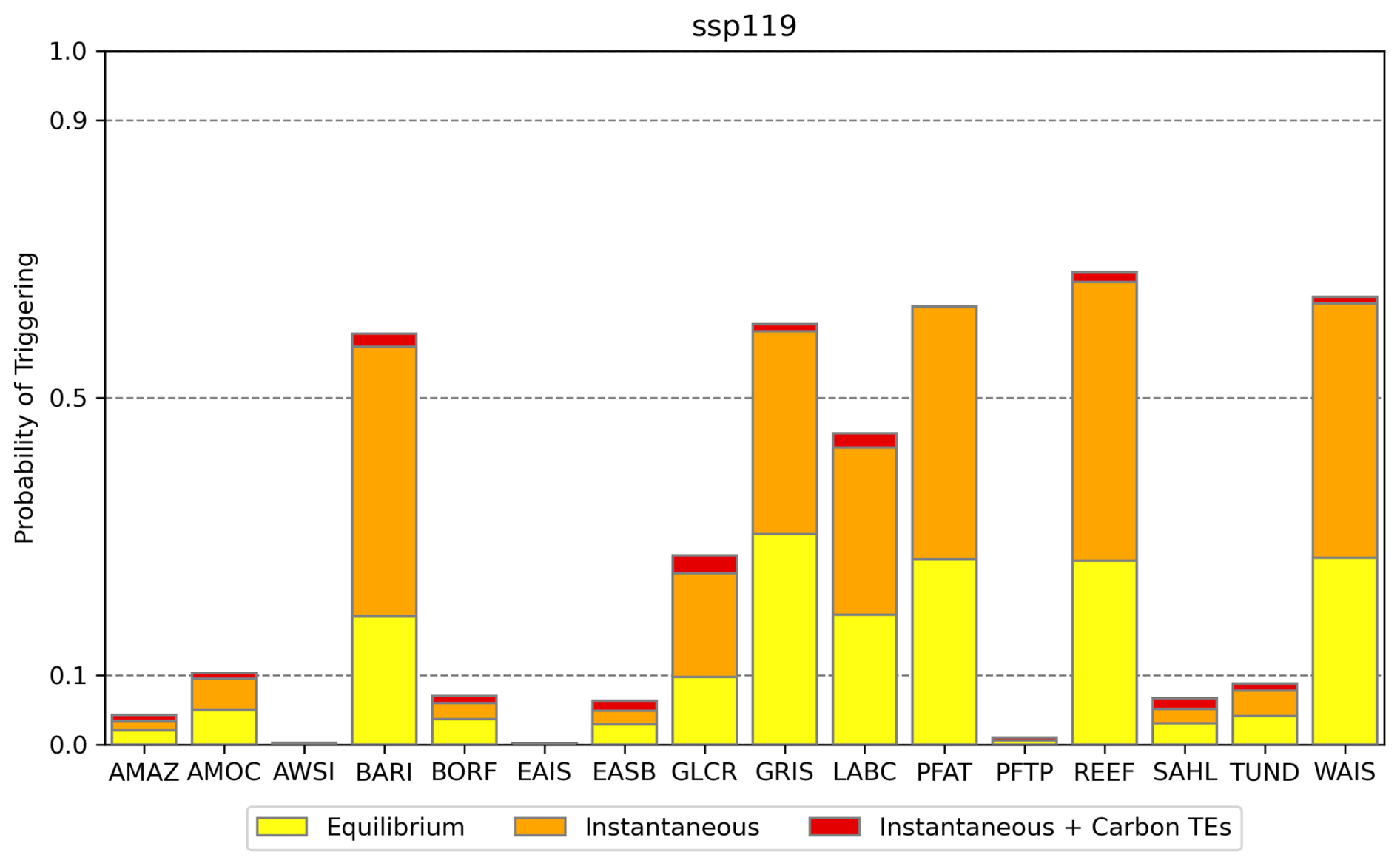
Figure 8 Probabilities of triggering the TEs under SSP1-1.9 for the case of equilibrium triggering, instantaneous triggering and instantaneous triggering including the additional warming from carbon TEs.

Under SSP5-8.5 the probability of triggering is highest among all SSPs with all three probability estimates agreeing on a probability of triggering of around 95 % averaged over all TEs (Table 3). The probability of triggering estimates is above 90 % for all TEs except AWSI and EAIS, which still remain at probabilities of triggering well above 50 % (Fig. 5). Even though the probabilities of triggering are reduced slightly under SSP3-7.0, the general picture remains the same (Table 3, Fig. S10). That the differences between the three probability estimates remain small under both SSP5-8.5 and SSP3-7.0 has two reasons: first, temperatures are increasing monotonously throughout the simulation period in almost all ensemble members (Fig. 4), causing the probability of equilibrium triggering to agree with the probability of instantaneous triggering. Second, temperatures well above the threshold temperatures of most TEs are reached even without the effect of carbon TEs; hence, their impact on the probability of triggering is almost negligible.

The probability of triggering TEs is still high under SSP2-4.5, with a probability of equilibrium triggering of 62 % averaged over all TEs. However, the probability of triggering varies strongly between the different TEs (Fig. 6). While BARI, GRIS, PFAT, REEF and WAIS are triggered with more than 90 % probability in all three cases, the probabilities of triggering AMOC, PFTP, TUND and AWSI remain below 50 % and even below 10 % for EAIS. Among all SSPs, SSP2-4.5 is the one with the highest increase in the probability of instantaneous triggering caused by additional warming from carbon TEs, with a 3 percentage point increase averaged over all TEs (Table 3). This matches our finding that the highest long-term temperature increase from carbon TEs is also possible under SSP2-4.5 (Table 2). However, compared to a baseline probability of instantaneous triggering of 64 %, the probability increase from carbon TEs remains small. Like under higher-emission scenarios, changing our assumption about the effective timescale of the TEs is not changing the probability of triggering estimates much under SSP2-4.5 (Table 3), since the temperature is increasing monotonously throughout the simulation period for most ensemble members (Fig. 4).

Inspecting the probabilities of triggering under SSP1-2.6 and SSP1-1.9, it becomes clear why it is important to distinguish between the concepts of equilibrium and instantaneous triggering. Under both scenarios, the temperature increase is no longer monotonous but includes a peak in the 21st century after which temperatures decline before they stabilise (Fig. 4). This causes the probability of instantaneous triggering, for which we assume an effective timescale of zero, i.e. instantaneous triggering once the threshold temperature is crossed, to be significantly higher than the probability of equilibrium triggering, for which we assume an effective timescale that is long compared to the overshoot time; i.e. triggering occurs only if the stabilised temperature is above the threshold temperature (Table 3). This difference between the probability of equilibrium and the probability of instantaneous triggering can be interpreted as a measure of the uncertainty in the probability of triggering arising from being unable to constrain the effective timescale more rigorously. Under both SSP1-1.9 and SSP1-2.6, this uncertainty is 1 order of magnitude higher than the additional probability of triggering caused by carbon TEs (Table 3).

Despite this uncertainty, it is clear that moving from SSP2-4.5 to SSP1-2.6 reduces the probability of triggering multiple TEs significantly (Table 3). No TE exceeds 90 % probability of getting triggered under SSP1-2.6 (Fig. 7). However, for the five TEs PFAT, REEF, GRIS, WAIS, and BARI all three probability estimates are higher than 50 %. The triggering of PFTP, AWSI and EAIS is unlikely under SSP1-2.6, with their probabilities of triggering remaining well below 10 %.

SSP1-1.9 is the scenario with the most pronounced temperature overshoot (Fig. 4) and hence the highest uncertainty arising from our assumption about the effective timescale of the TEs. Averaged over all TEs, the probability of instantaneous triggering is more than twice as high as the probability of equilibrium triggering (Table 3). Nevertheless, it is safe to say that SSP1-1.9 is the scenario that minimises the risk of triggering TEs. No TE has a probability of equilibrium triggering above 50 %, and for eight TEs the probabilities of triggering remain under 10 % (Fig. 8).

6 Discussion

With CTEM we introduce a simplistic model which is able to represent carbon emissions from the three carbon TEs PFAT, PFTP and AMAZ in line with the estimates from Armstrong McKay et al. (2022). However, the impacts from the carbon TEs estimated in this study remain somewhat speculative, as there is only limited confidence about the actual existence of tipping points within the carbon TEs, with low confidence for PFTP and medium confidence for PFAT and AMAZ (Table 1). The distinction between PFGT, PFAT and PFTP made by Armstrong McKay et al. (2022) for permafrost thaw also remains questionable. Most studies, including the latest IPCC report, assume that permafrost thaw can be divided into gradual and abrupt thaw processes, corresponding to PFGT and PFAT, and do not mention permafrost collapse due to compost bomb instabilities (PFTP) (e.g. Canadell et al., 2021; Turetsky et al., 2020; Schuur et al., 2015; Wang et al., 2023). Since PFTP causes the highest carbon emissions of all three carbon TEs with up to 250 Gt C (Table 1), the impact of tipping elements within the carbon cycle will be less severe than found in this study if PFTP does not include a tipping point.

Yet, additional carbon emissions released by gradual permafrost thaw under continued global warming of up to 260 Gt C (Table 1) need to be expected, which are not considered in this study. One reason to exclude PFGT is that it is not assumed to include tipping points but to be a threshold-free feedback to global warming (Armstrong McKay et al., 2022). Furthermore, sophisticated models of PFGT already exist (e.g. Gasser et al., 2018; Burke et al., 2020); hence, it would not be appropriate to represent PFGT with a simple conceptual model like CTEM.

It is challenging to compare the carbon emissions from carbon TEs identified by us to other studies, as this is to the best of our knowledge the first study to investigate the impact of all TEs within the carbon cycle. Other studies only analyse single TEs, e.g. Cox et al. (2004) and Parry et al. (2022) for AMAZ or Schneider von Deimling et al. (2015) and Gasser et al. (2018) for permafrost thaw as a whole. Since the individual carbon emissions from the carbon TEs modelled by CTEM are based on the estimates of Armstrong McKay et al. (2022), we could only reproduce their analysis by comparing our individual carbon emission estimates to the literature. Nevertheless, it must be noted that even though the uncertainty ranges of the carbon impacts identified by Armstrong McKay et al. (2022) based on numerous studies are large (factor of 2 for PFTP and AMAZ, factor of 3 for PFAT), they do not include all estimates from the literature. Especially the lower bounds of AMAZ and PFTP are questionable. Carbon emissions from the Yedoma region, which make up the major part of PFTP emissions, of only 23 Gt C in 2300 under RCP5-8.5 have been found by an observations-based modelling study (Schneider von Deimling et al., 2015). This is much lower than the minimum carbon emissions of 100 Gt C from the Yedoma region assumed by Armstrong McKay et al. (2022), which led to an estimated minimum impact of PFTP of 125 Gt C. The minimum impact of 30 Gt C for AMAZ might also be too high since no substantial carbon loss from AMAZ is observable in CMIP6 models, even if localised dieback occurs (Parry et al., 2022). Given that the emission estimates from Armstrong McKay et al. (2022) used to parameterise CTEM seem to be on the high side compared to other studies, we are confident about our finding that the warming caused by carbon TEs on average remains small compared to the anthropogenic warming.

The timing of triggering carbon TEs and hence their impact on global warming derived by us is potentially biased towards early times, since we assume instantaneous triggering within CTEM. A more realistic model should include the sluggish behaviour of carbon TEs marked by effective timescales longer than zero. Since this bias would also cause an overestimation of the warming caused by carbon TEs, it does not reduce the confidence in our finding that the warming caused by carbon TEs on average remains small compared to the anthropogenic warming.

The three estimates of the probability of triggering allow us to analyse how probabilities of triggering might be amplified by carbon TEs and how large the respective uncertainties are that result from not knowing the effective timescales of the TEs. While it is clear that the amplification of probabilities of triggering from carbon TEs remains small, the uncertainty arising from not knowing the effective timescale is large for scenarios that include a temperature overshoot (Table 3). The internal timescale of a TE as defined by Armstrong McKay et al. (2022) can give a first indication of whether its probability of triggering will be closer to the probability of instantaneous triggering (short internal timescale) or equilibrium triggering (long internal timescale). It is this approach that Wunderling et al. (2023) follow to include the timescales of TEs in their analysis. However, we think that further research is necessary to better understand the timing of triggering TEs.

The probabilities of triggering derived by us might be slightly overestimated, since the climate sensitivity of FaIRv2.0.0 is not well constrained towards its upper limit (Leach et al., 2021). This is a result of this version of FaIR not being calibrated to match the IPCC range of climate sensitivity. This has been fixed in later versions of the model which we were not aware of when conducting this study. Nevertheless, we regard this possible overestimation to be small, since the median climate sensitivity of Fairv2.0.0 agrees well with the latest IPCC estimate (Forster et al., 2021).

Given the sluggish behaviour of TEs, it is interesting to inspect long time horizons to determine the probability of triggering. This is why we base our analysis beyond 2100 on the emission scenario extensions from Meinshausen et al. (2020). However, they are not backed by integrated assessment modelling (IAM) studies. To derive a more realistic estimate for the risk of triggering TEs that society might face, it would be interesting to generate IAM-backed emission scenarios beyond 2100.

Comparing our probability of triggering estimates to the results of Kriegler et al. (2009), which have found much use in the climate tipping point literature (e.g. Lontzek et al., 2015; Cai et al., 2015, 2016), is tricky, since their expert assessment focuses on the year 2200, while our results do not target a specific time horizon. They provide ranges of probabilities of triggering for the year 2200 under three warming scenarios: a low-temperature corridor comparable to SSP1-1.9, a medium-temperature corridor comparable to SSP2-4.5 and a high-temperature corridor comparable to SSP3-7.0. For the medium-temperature corridor, Cai et al. (2016) infer mean probabilities of triggering from the ranges given in Kriegler et al. (2009) of 22 % for AMOC, 52 % for GRIS, 34 % for WAIS and 48 % for AMAZ. Even our most conservative probability estimate assuming equilibrium triggering is significantly higher for most TEs under SSP2-4.5 with 39 % for AMOC, 93 % for GRIS, 96 % for WAIS and 44 % for AMAZ (Fig. 6).

We think that those deviations are not mainly an artefact of the different treatment of time horizons but are rooted in new scientific literature published since Kriegler et al. (2009), which provides the basis for the threshold temperature estimates from Armstrong McKay et al. (2022) that our calculation of triggering probabilities is largely based on. The increased triggering probability for AMOC can be linked to various studies reporting the unrealistic stability of AMOC in general circulation models (GCMs) (e.g. Liu et al., 2017), together with empirical evidence for the loss of stability of AMOC (Boers, 2021). New indications for the proximity of a tipping point for GRIS are also derived from observations of ice loss (King et al., 2020; Boers and Rypdal, 2021), with recent modelling studies confirming this (Van Breedam et al., 2020; Robinson et al., 2012; Bochow et al., 2023). The loss of WAIS is becoming observable (Shepherd et al., 2019), and a tipping point might already be crossed with several glaciers in the Amundsen Sea currently undergoing marine ice sheet instability (Rignot et al., 2014).

Even though we find an increase in the probabilities of triggering caused by the additional carbon emissions from carbon TEs, this impact is not strong enough to trigger any tipping cascades and remains small compared to the scenario dependence of tipping probabilities. Even under SSP2-4.5, which features the highest long-term increase in temperature of up to 0.91 °C due to carbon emissions from carbon TEs, the additional probability of instantaneous triggering caused by this temperature increase is only 3 percentage points on average. Despite our finding that the impact from carbon TEs alone is too small to trigger tipping cascades, tipping cascades might still emerge as major physical interactions between TEs aside from carbon emissions are not accounted for in this study (Wunderling et al., 2021).

It must also be noted that our findings critically depend on the assessment of climate tipping points by Armstrong McKay et al. (2022). However, we believe that this study best summarises the current state of knowledge about climate tipping points, relying on more than 300 references. Narrowing the uncertainty range of threshold temperatures is an enormous task for future research, which would allow for more precise statements about the probability of triggering climate TEs.

7 Conclusions

We developed a simple model framework to explore the probabilities of triggering climate TEs and how they are amplified by carbon emissions from carbon TEs under five SSPs.

We show that the additional carbon emissions from carbon TEs increase the risk for high-temperature pathways, especially under SSPs with comparably low anthropogenic carbon emissions. On average, however, the additional warming from carbon TEs remains low compared to the anthropogenic warming. Therefore, the probability of triggering climate TEs is to first order determined by the emission scenario and not by whether carbon TEs are triggered or not. Consistent with this, we also do not see any tipping cascades being triggered by carbon TEs.

The uncertainty about the effective timescale of TEs makes it hard to estimate the probability of triggering for scenarios including a temperature overshoot. This is most pronounced under SSP1-1.9, for which the probabilities of triggering more than double if we switch from the conservative assumption that the effective timescales are long compared to the temperature overshoot time to the assumption that the TE is triggered instantaneously once the threshold temperature is crossed.

Despite this uncertainty, it is clear that current policies, steering towards a pathway comparable to SSP2-4.5 (Climate Action Tracker, 2022; United Nations Environment Programme, 2022; Meinshausen et al., 2022), are highly unsafe with regard to triggering climate tipping points. The triggering of multiple TEs is likely under SSP2-4.5 with a 64 % probability of instantaneous triggering on average over all 16 TEs. The temperature increase from carbon TEs increases this number by 3 percentage points, which is the highest probability increase caused by carbon TEs among all SSPs. This is in line with the highest long-term temperature increase caused by carbon TEs becoming possible under SSP2-4.5, with values reaching from 0.03 to 0.91 °C in 2500 (5th to 95th percentile range). Moving from SSP2-4.5 to SSP1-2.6 reduces the probability of triggering TEs substantially, with an average probability of instantaneous triggering of 37 % under SSP1-2.6. The impact of carbon TEs is also less severe under this scenario, ranging from 0 to 0.54 °C, which leads to an increase in the average probability of triggering of 2 percentage points.

The probabilities of triggering climate TEs derived by us are higher than the estimates from the often-cited expert elicitation conducted by Kriegler et al. (2009). This is explained by recent evidence for the proximity of climate tipping points, leading to low estimates of the respective threshold temperatures.

If the risk of triggering TEs is to be reduced, rapid action is needed to reduce greenhouse gas emissions, since climate tipping points are already close, and it will be decided within the coming decades if they will be crossed or not.