A saddle-node bifurcation may be causing the AMOC collapse in the Community Earth System Model

Recently, a collapse of the Atlantic Meridional Overturning Circulation (AMOC) was found in the Community Earth System Model (CESM) under constant pre-industrial greenhouse gas forcing conditions. To determine the stability changes of the AMOC with changing (freshwater) parameters in models, it is important to determine the origin of the collapse behavior. In this paper, we argue that the classical picture of a saddle-node bifurcation holds for the AMOC collapse in the CESM. We provide specific supporting arguments by showing results of additional pre-industrial CESM simulations. The CESM results are compared with those of a five-box AMOC model, which is known to have saddle-node bifurcations, and with which many sensitivity experiments can be performed. Theoretical arguments are also provided showing that the essential dynamics of the CESM can be reduced to a low-dimensional model in which a saddle-node bifurcation causes the AMOC collapse. The underlying physical reason is that the AMOC behaviour in CESM is controlled by a small set of dominant feedback processes. This has important consequences for the value of conceptual AMOC models, for assessing the effect of model biases on the AMOC stability, and for the interpretation of AMOC behaviour under climate change scenarios.

1 Introduction

A hot issue in current climate research is the Atlantic Meridional Overturning Circulation (AMOC) response under future climate change. Climate models participating in the Coupled Model Inter-comparison Project Phase 6 (CMIP6, Eyring et al., 2016) indicate a substantial AMOC weakening during the 21st century (Weijer et al., 2020). Beyond 2100 there is much more uncertainty as the AMOC may (partially) recover or fully collapse (Liu et al., 2017; Bonan et al., 2022; Drijfhout et al., 2025). Transient temperature responses are effective in causing the 21st century AMOC weakening but salinity responses are crucial in further destabilizing the AMOC (Gérard and Crucifix, 2024; van Westen et al., 2025b). The dominant destabilizing AMOC tipping mechanism is the salt-advection feedback, where an AMOC weakening leads to a smaller northward salinity transport amplifying the initial AMOC weakening (e.g., Marotzke, 2000). The existence of the salt-advection feedback is why the AMOC is labelled as a tipping point in the climate system (Lenton et al., 2008; Armstrong McKay et al., 2022).

Stommel (1961) was the first to identify the salt-advection feedback in a simple two-box model and demonstrated that this feedback induces transitions between two stable AMOC steady states. The multi-stable AMOC regime is bounded by two saddle-node bifurcations in this model. Since then, studies using more detailed conceptual (box) models (Cessi, 1994; Cimatoribus et al., 2014; Wood et al., 2019) and numerically fully-implicit ocean-climate models (De Niet et al., 2007; Toom et al., 2012; Mulder et al., 2021) have shown that saddle-node bifurcations bound the multi-stable regime of the AMOC in these models. Rahmstorf (1996) showed that the saddle-node bifurcation associated with the AMOC collapse is linked to a critical value of the freshwater transport carried by the AMOC at 34° S, represented by the quantity F_ovS. When including the stabilizing gyre responses (Sijp, 2012), a F_ovS minimum is found close to this saddle-node bifurcation (Dijkstra, 2007).

In numerically explicit ocean-climate models it is much harder (or not feasible) to determine the steady states versus (freshwater forcing) parameters and the boundaries of the AMOC multi-stable regime. An impression of the multi-stable regime can be obtained by performing quasi-equilibrium simulations, where a freshwater flux forcing is changed very slowly back-and-forth such that the model state stays close to the (slowly changing) statistical equilibrium. Such quasi-equilibrium simulations have been performed with many ocean-only models (Rahmstorf, 1995; Lohmann et al., 2024), Earth System Models of Intermediate Complexity (EMICs) (Rahmstorf et al., 2005; Cini et al., 2024), the FAMOUS model (Hawkins et al., 2011), the Community Climate System Model (CCSM3) (Hu et al., 2012), and recently in the Community Earth System Model (CESM) (van Westen and Dijkstra, 2023; van Westen et al., 2024a).

When the salt-advection feedback is the dominant feedback, as is the case for the Stommel (1961) model, it can be shown that the stable “AMOC on” state has a square-root (or quadratic) solution against varying freshwater flux forcing (see Appendix A) with the normal (most simple) form of $\mathrm{d}x/\mathrm{d}t=r-x^{\mathrm{2}}$ with r>0 (see Appendix B). This square-root relation in the Stommel model can be understood from the fact that the AMOC strength is proportional to the salinity gradient, whereas the salinity gradient is also proportional to the AMOC strength. In more complex (climate) models that resolve more processes and climate feedbacks, a near square-root dependency is also found for the AMOC strength against forcing (Dijkstra, 2007; van Westen et al., 2024b; Vanderborght et al., 2025). Finding indications of a square-root relation in quasi-equilibrium simulations is challenging as it requires very slow rates to follow the steady states of the system (Rahmstorf, 1996). Even if the rate is sufficiently slow, this relation can be masked by relatively large (stochastic) noise (Berglund and Gentz, 2006). An alternative approach is by obtaining statistical equilibria for fixed forcing values, but this is computationally too costly for CESM. Nevertheless, as long as the salt-advection feedback remains dominant amid other AMOC-related feedbacks (Vanderborght et al., 2025), a square-root dependency can be expected when the system is relatively close to its saddle-node bifurcation and hence to tipping.

Here, we focus on the CESM results and address the issue whether its AMOC tipping behavior is also caused by the presence of a saddle-node bifurcation, similar to that in the fully-implicit ocean-climate models (Dijkstra, 2007). This is certainly a non-trivial issue as the CESM is an extremely high-dimensional dynamical system and the atmospheric fluxes create a high frequency forcing on the ocean component of the model. In addition, in the quasi-equilibrium CESM simulation (van Westen et al., 2024a) the forcing rate is rather large compared to the equilibration time scale of the AMOC (van Westen et al., 2024b) and hence the (non-autonomous) dynamical system is not a fast-slow system (Kuehn, 2011). The existence of a saddle-node bifurcation in the CESM is important for assessing the role of model biases on the stability of the AMOC and for understanding the response of the model to transient climate change forcing (Ritchie et al., 2021).

The aim of this paper is to provide a convincing case that a saddle-node bifurcation is causing the AMOC collapse in the CESM, as presented in van Westen et al. (2024a). Thereto, we have performed several additional CESM simulations which were branched from the quasi-equilibrium CESM simulation, we will compare the CESM behavior with that of a five-box AMOC model for which a saddle-node bifurcation is known to exist (van Westen et al., 2024b). The advantage of this five-box model is that we can easily conduct multiple sensitivity experiments to better understand the CESM behaviour. Section 2 describes the model set-up and simulations for the CESM and five-box model. Next, in Sect. 3, the results on the (statistical) steady states and quasi-equilibrium results of both the CESM and five-box model are presented. Section 4 provides detailed arguments for the existence of a saddle-node bifurcation in the CESM, followed by Sect. 5, where the importance of this result for the behavior of the AMOC under climate change is shown. Finally, in Sect. 6, the results are summarized and discussed.

2 Models and Methods

2.1 CESM simulations

The CESM (version 1.0.5) is a fully-coupled climate model and the simulations here have a 1° horizontal resolution for the ocean/sea-ice components and a 2° horizontal resolution for the atmosphere/land components. For more details on the precise CESM set-up, we refer to van Westen and Dijkstra (2023) and van Westen et al. (2024a). In those studies, the pre-industrial forcing is used and in addition a freshwater flux forcing (F_H) is applied between 20° N and 50° N in the Atlantic Ocean and is compensated elsewhere (at the ocean surface) to conserve salinity. This is the same hosing region as in Hu et al. (2012) and Rahmstorf (1996), which has the advantage that the North Atlantic deep convection sites are not directly impacted under the hosing. The sensitivity of the hosing location will be thoroughly analysed below for the five-box AMOC model.

The quasi-equilibrium AMOC hysteresis simulation (van Westen and Dijkstra, 2023) is obtained by slowly increasing F_H from 0 to 0.66 Sv and back to 0 Sv, at a rate of $\mathrm{3}\times {\mathrm{10}}^{-\mathrm{4}}$ Sv yr⁻¹, resulting in a 4400-year long simulation. This simulation remains close to the statistical equilibria, but the deviations become larger near the AMOC collapse and recovery (van Westen et al., 2024b). To determine statistical equilibria (i.e., steady states), two 500-year long CESM simulations were performed (van Westen et al., 2024b) at constant F_H, the steady states are indicated as $\stackrel{\mathrm{‾}}{F_H}$. This was already done for $\stackrel{\mathrm{‾}}{F_H}=\mathrm{0.18}$ Sv (starting at model year 600 of the quasi-equilibrium simulation) and at $\stackrel{\mathrm{‾}}{F_H}=\mathrm{0.45}$ Sv forcing (starting at model year 1500). The last 100 years of these steady states show hardly any model drift, meaning that the AMOC and global climate are dominated by natural climate variability (van Westen and Baatsen, 2025). Below, we will show results of new CESM simulations performed under constant $\stackrel{\mathrm{‾}}{F_H}$ forcing or with a slower rate of F_H, and closer to the values where the AMOC collapse occurs in the quasi-equilibrium simulation (around F_H=0.525 Sv, van Westen et al. (2024a)).

We will (in Sect. 5) also use results from two climate change simulations that were initialized from the end of the steady state with $\stackrel{\mathrm{‾}}{F_H}=\mathrm{0.18}$ Sv and $\stackrel{\mathrm{‾}}{F_H}=\mathrm{0.45}$ Sv (van Westen et al., 2025b). These climate change simulations were first forced under the historical forcing (1850–2005) and followed by either RCP4.5 or RCP8.5 scenario forcing (2006–2100, Representative Concentration Pathway). Subsequently, they were further integrated for 400 years under their 2100 radiative forcing conditions to study the equilibrium behaviour.

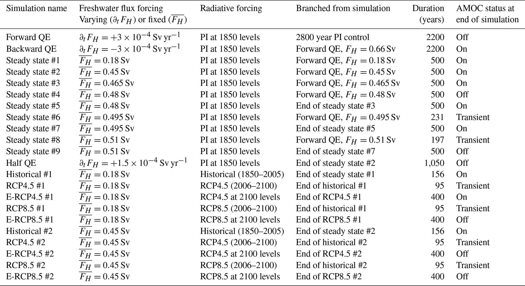
An overview of all the different CESM simulations are presented below in Table 1. In total, we present 11 670 model years of model output. Ideally, one would determine even more steady states or lower the varying F_H rate in the quasi-equilibrium simulation, but this is computationally not feasible. These additional simulations, however, can be done with the five-box AMOC model.

Table 1 Overview of the different simulations conducted with the CESM, which includes: simulation name, freshwater flux forcing (varying or fixed), radiative forcing, branched from simulation, duration, and the AMOC status at the end of simulation (on, transient or off). Note that the forward QE was branched from the 2800-year long pre-industrial control simulation from Baatsen et al. (2020). The simulations are sorted in order of appearance. Abbreviations: QE, quasi-equilibrium; PI, pre-industrial; RCP, Representative Concentration Pathway; E-RCP, Extended Representative Concentration Pathway.

2.2 The five-box AMOC model

The five-box AMOC model (Fig. 1) was developed by Cimatoribus et al. (2014), extended by Castellana et al. (2019), and was recently further extended (hereafter the E-CCM, the Extended Cimatoribus-Castellana Model) by including oceanic temperatures (van Westen et al., 2024b). The E-CCM has four surface boxes, where the Atlantic Ocean is represented by boxes t and n, the Southern Ocean channel by box s, and the Southern Ocean Atlantic sector by box ts. There is one deep ocean box d, hence this model does not include the Indo-Pacific Ocean nor Arctic Ocean. The Atlantic Ocean pycnocline depth, indicated by the D, may vary in the E-CCM. The temperature and salinity are volume averaged over each box and heat and salinity are exchanged between the boxes, and also heat between the surface boxes and overhead atmosphere. Salinity is conserved in the E-CCM.

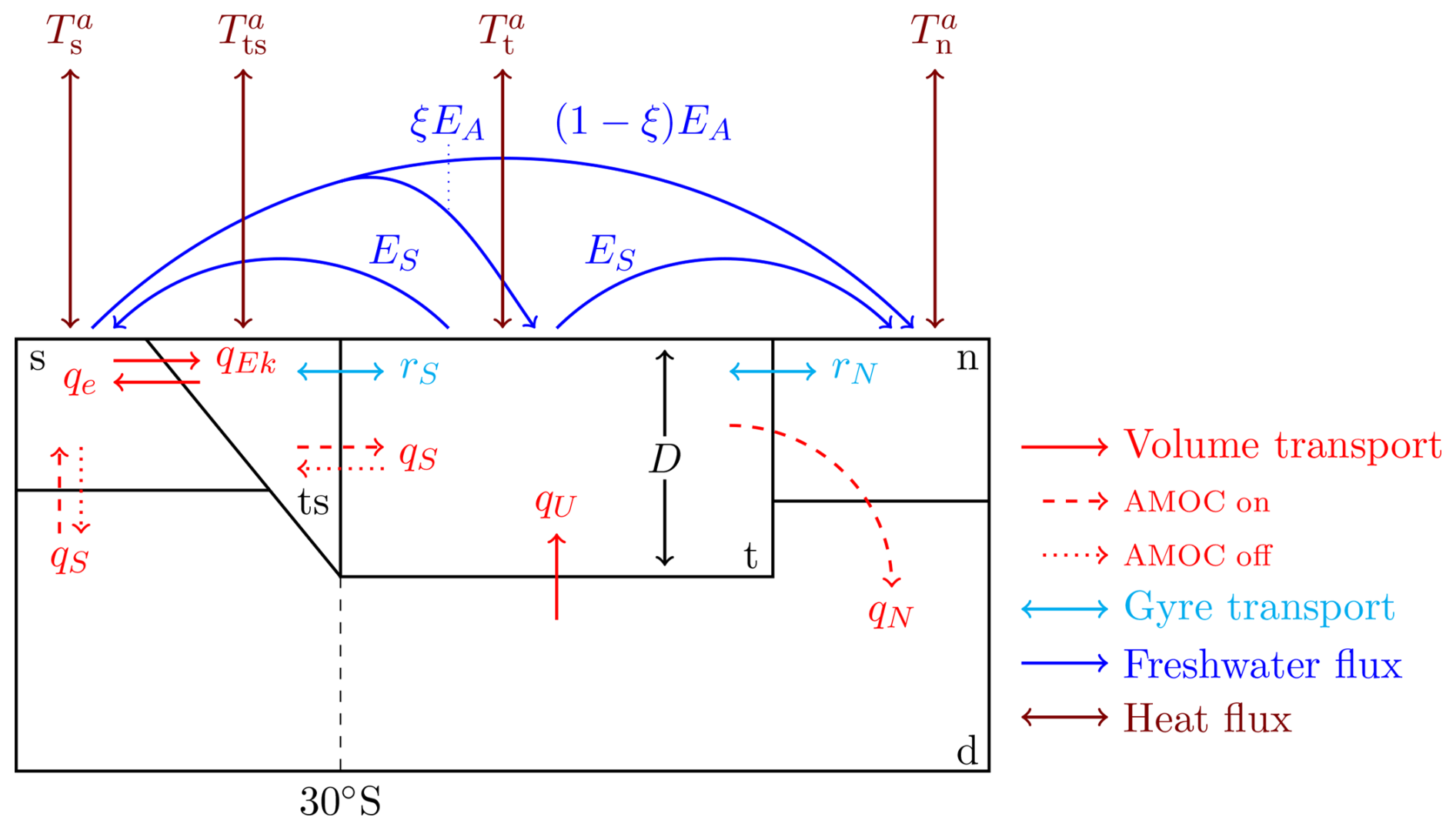
Figure 1 Schematic representation of the five-box AMOC model (the E-CCM), adapted from van Westen et al. (2024b). The red arrows represent volume transports, whereas the dashed and dotted arrows indicate the AMOC on and AMOC off states, respectively. The cyan and blue arrows represent the gyre transport and freshwater fluxes, respectively. The freshwater from box s is distributed linearly over box n and box t using a parameter ξ, where ξE_A is added to box t and (1−ξ)E_A to box n. The original E-CCM configuration van Westen et al. (2024b) is obtained when ξ=0. The brown arrows are the heat fluxes with the overhead atmosphere for each surface box (i.e., box s, ts, t and n).

The AMOC strength in the northern box (q_N) in the E-CCM is given by:

$$\begin{array}{}\text{(1)}& q_{\mathrm{N}}={\mathit{\eta }}_{\mathrm{h}}{\displaystyle \frac{{\mathit{\rho }}_{\mathrm{n}}-{\mathit{\rho }}_{\mathrm{ts}}}{{\mathit{\rho }}_{\mathrm{0}}}}{D}^{\mathrm{2}},\end{array}$$

where η_h is a hydraulic constant, ρ_n−ρ_ts is the meridional density difference between box n and box ts, ρ₀ is a reference density, and D the pycnocline depth. The densities are determined from a linear equation of state. For full details and sensitivity experiments conducted with the E-CCM, we refer to van Westen et al. (2024b), where there is also a link to the publicly-available E-CCM code. We will show results for the version where sea-ice insulation effects are omitted and use the standard values of the parameters given in van Westen et al. (2024b), unless otherwise mentioned.

The E-CCM is forced through the asymmetric freshwater flux forcing (E_A) from box s to box n. Under varying E_A, the E-CCM has an “AMOC on” state (clockwise circulation, red solid and dashed arrows) and an “AMOC off” state (anti-clockwise circulation, red solid and dotted arrows). There is a multi-stable AMOC regime and this regime is bounded by two saddle-node bifurcations (van Westen et al., 2024b). To determine the sensitivity of the AMOC behavior to the hosing location (Rahmstorf, 1996; Ma et al., 2024), we make a modification to the E-CCM by distributing the freshwater flux forcing linearly over box n and box t using a parameter $\mathit{\xi }\in [\mathrm{0},\mathrm{1}]$. When ξ=0, the freshwater flux forcing is only applied to box n and this is the original E-CCM configuration. The freshwater flux forcing is only over box t when ξ=1.

The steady states of the E-CCM against varying parameters (i.e., bifurcation diagram), such as freshwater flux forcing, are determined using the continuation software AUTO-07p (Doedel et al., 2007, 2021). This code solves steady states using a pseudo-arclength continuation combined with a Newton-Raphson method (Wubs and Dijkstra, 2023). It is also able to detect Hopf bifurcations and saddle-node bifurcations. We used a value of 10⁻⁶ for the absolute and relative accuracy of each steady-state solution, and for the accuracy for locating special points, similar to van Westen et al. (2024b).

3 Results

3.1 Statistical equilibria in the CESM

The AMOC strength (at 1000 m and 26° N) and the freshwater transport carried by the AMOC at 34° S (F_ovS) of the quasi-equilibrium CESM simulation (van Westen et al., 2024a) are shown in Fig. 2a, b. The branched simulations from the quasi-equilibrium simulation at a constant forcing $\stackrel{\mathrm{‾}}{F_H}=\mathrm{0.18}$ Sv (Fig. 2c, i), $\stackrel{\mathrm{‾}}{F_H}=\mathrm{0.45}$ Sv (Fig. 2d, j) and $\stackrel{\mathrm{‾}}{F_H}=\mathrm{0.465}$ Sv (Fig. 2e, k) equilibrate after about 300 years. The branched simulation at $\stackrel{\mathrm{‾}}{F_H}=\mathrm{0.48}$ Sv (Fig. 2f, l) collapses and suggests that the upper bound of the multi-stable regime is around this $\stackrel{\mathrm{‾}}{F_H}$ value. The branches initiated from $\stackrel{\mathrm{‾}}{F_H}=\mathrm{0.495}$ Sv (Fig. 2g, m) and $\stackrel{\mathrm{‾}}{F_H}=\mathrm{0.51}$ Sv (Fig. 2h, n) also collapse; these simulations were terminated before the 500-year mark because of computational costs. However, when the equilibrated $\stackrel{\mathrm{‾}}{F_H}=\mathrm{0.465}$ Sv simulation is subjected to an instantaneous increase in freshwater flux to $\stackrel{\mathrm{‾}}{F_H}=\mathrm{0.48}$ Sv ($\mathrm{\Delta }\stackrel{\mathrm{‾}}{F_H}=\mathrm{0.015}$ Sv), we still find a statistical equilibrium in the northward overturning regime (red curves in Fig. 2f, l). We iteratively repeated the same procedure for $\stackrel{\mathrm{‾}}{F_H}=\mathrm{0.495}$ Sv and $\stackrel{\mathrm{‾}}{F_H}=\mathrm{0.51}$ Sv. The AMOC eventually collapses under a constant freshwater flux forcing of $\stackrel{\mathrm{‾}}{F_H}=\mathrm{0.51}$ Sv. This means that the upper bound of the multi-stable regime is found for 0.495 Sv$\le \stackrel{\mathrm{‾}}{F_H}<$ 0.51 Sv. To obtain an even higher precision for this upper bound, we would need to increase $\stackrel{\mathrm{‾}}{F_H}$ with even smaller increments, but is not done here because of computational limitations.

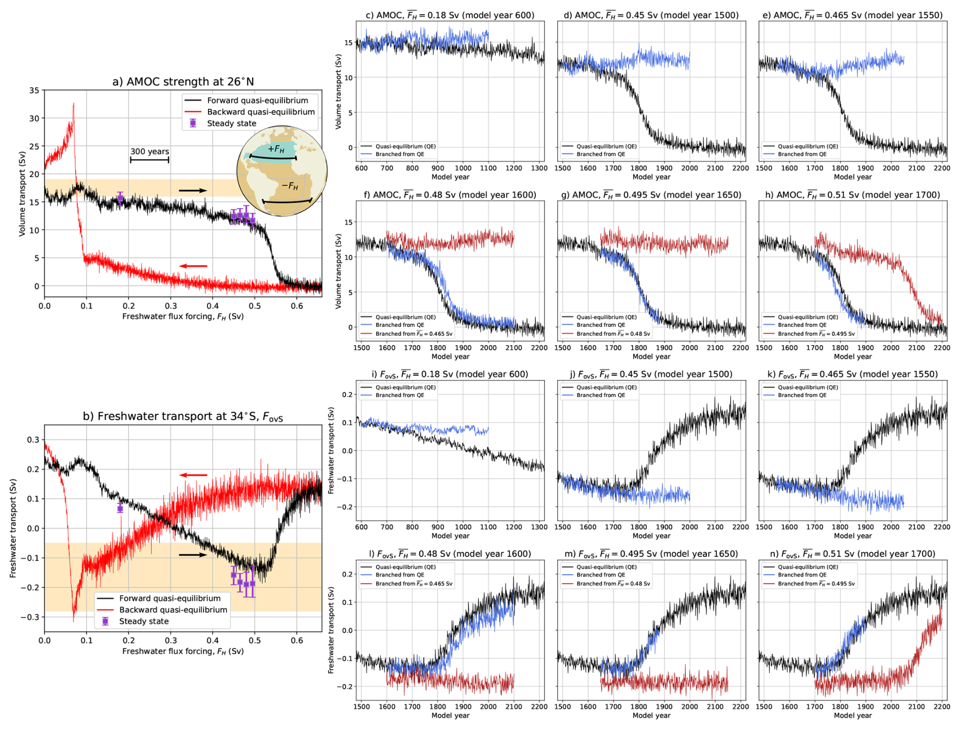
Figure 2 (a) The AMOC strength at 1000 m and 26° N and (b) the freshwater transport by the AMOC at 34° S, F_ovS, for varying freshwater flux forcing F_H (i.e., the quasi-equilibrium simulation). Inset: The hosing experiment where fresh water is added to the ocean surface between 20–50° N in the Atlantic Ocean (+F_H) and is compensated over the remaining ocean surface (−F_H). The statistical equilibria for various constant values of F_H (i.e., $\stackrel{\mathrm{‾}}{F_H}$, steady states) in the northward overturning regime are also shown, where the marker indicates the mean and the error bars show the minimum and maximum over the last 50 years of the 500-year long branched simulations. The black sections indicate the 26° N and 34° S latitudes over which the AMOC strength and F_ovS are determined, respectively. The yellow shading in the two panels indicates observed ranges for the presented quantity (Smeed et al., 2018; Arumí-Planas et al., 2024). (c–n) Similar to panels a,b, but now the entire branched simulations for different $\stackrel{\mathrm{‾}}{F_H}$ values. The branches are initiated from the quasi-equilibrium simulation (blue curves) or from the end of the previous statistical equilibria (red curves).

The AMOC in the quasi-equilibrium simulation starts to tip around F_H=0.525 Sv (0.522 to 0.533 Sv, 10th and 90th percentiles, van Westen et al. (2024a)) and is at larger F_H values than the upper bound found from the statistical equilibria simulation (0.495 Sv$\le \stackrel{\mathrm{‾}}{F_H}<$ 0.51 Sv). To determine the overshoot of the quasi-equilibrium simulation, we use a reference value of $\stackrel{\mathrm{‾}}{F_H}=\mathrm{0.5}$ Sv, but any other $\stackrel{\mathrm{‾}}{F_H}$ value within the interval $\stackrel{\mathrm{‾}}{F_H}\in [\mathrm{0.495},\mathrm{0.51}]$ can be used as a reference (giving slightly different numerical results). Using this reference, the quasi-equilibrium AMOC overshoots by ΔF_H=0.025 Sv (≈ 80 years). Do note that the AMOC collapses for the simulations branched from the quasi-equilibrium simulation for $\stackrel{\mathrm{‾}}{F_H}\ge \mathrm{0.48}$ Sv (blue curves in Fig. 2c–n). In other words, the branched simulations for $\stackrel{\mathrm{‾}}{F_H}\ge \mathrm{0.48}$ Sv already surpassed a critical forcing value upon branching, which means that the standard quasi-equilibrium also surpassed its critical value and actually undershoots the upper bound of the multi-stable regime. This critical value for the quasi-equilibrium is located for 0.465 Sv $<\stackrel{\mathrm{‾}}{F_H}\le$ 0.48 Sv. The apparent overshoot with the reference value of $\stackrel{\mathrm{‾}}{F_H}=\mathrm{0.5}$ Sv is then the result of inertia and the growth rate of AMOC feedbacks, in particular the destabilising salt-advection feedback. Indeed, these feedbacks develop on centennial timescales (Vanderborght et al., 2025), which we will make more explicit below. The undershooting AMOC can already be seen when comparing the quasi-equilibrium with five different statistical equilibria (last 50 model years are used). The quasi-equilibrium simulation is about 1 Sv weaker than the statistical equilibria, but still reasonably agree. For F_ovS, on the other hand, the quasi-equilibrium is larger and (mostly) outside the ranges of the different statistical equilibria (Fig. 2b).

When we lower the freshwater flux forcing rate, we expect that the system stays closer to the statistical equilibria (Hawkins et al., 2011). To test this, we branched off a quasi-equilibrium simulation with only half the hosing rate (i.e., $\mathrm{1.5}\times {\mathrm{10}}^{-\mathrm{4}}$ Sv yr⁻¹) from the end of the statistical equilibrium at $\stackrel{\mathrm{‾}}{F_H}=\mathrm{0.45}$ Sv. This simulation was integrated for 1,050 model years, where F_H varied from 0.45 Sv to 0.608 Sv (red curves in Fig. 3a, b). In the ideal case, the half-forcing quasi-equilibrium simulation should have been initiated from the same initial conditions as the standard quasi-equilibrium simulation for direct comparison, which would also allow to address the sensitivity in the overshoot/undershoot with the reference value of $\stackrel{\mathrm{‾}}{F_H}=\mathrm{0.5}$ Sv. Nevertheless, this half-forcing simulation can be used to check whether the AMOC collapse happens faster in F_H space. The faster transition (in F_H) is a characteristic of a saddle-node bifurcation (see Appendix B), but this is also the case for other bifurcation types (e.g., Hopf) (Berglund and Gentz, 2006).

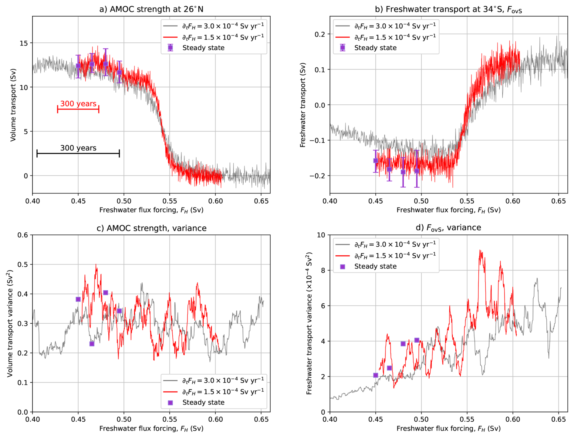
Figure 3 (a , b) The AMOC strength and F_ovS of the quasi-equilibrium simulations, one similar to Fig. 2a, b, and including the simulation with varying $\mathrm{1.5}\times {\mathrm{10}}^{-\mathrm{4}}$ Sv yr⁻¹ hosing rate (red curves). This quasi-equilibrium hosing with $\mathrm{1.5}\times {\mathrm{10}}^{-\mathrm{4}}$ Sv yr⁻¹ was branched from the end of the statistical equilibria at $\stackrel{\mathrm{‾}}{F_H}=\mathrm{0.45}$ Sv. (c, d) The variance in AMOC strength and F_ovS, using a sliding window of 50 years. For each 50-year window, a linear trend was removed and then the variance was determined.

The half-rate simulation remains (very) close to the different statistical equilibria for both AMOC strength and F_ovS. Following van Westen et al. (2024a), we used a break regression analysis (Mudelsee et al., 2014) to find the AMOC tipping event at F_H=0.534 Sv, with the 10th and 90th percentiles at F_H = 0.533 Sv and F_H = 0.536 Sv, respectively. There is an overshoot of ΔF_H=0.034 Sv (227 years) compared to our reference value of $\stackrel{\mathrm{‾}}{F_H}=\mathrm{0.5}$ Sv, but keep in mind that AMOC feedbacks take a considerable time to develop. These feedbacks can be quantified by following the procedure outlined in Vanderborght et al. (2025), see also Sect. 4 below. We decompose the different AMOC feedbacks for the $\stackrel{\mathrm{‾}}{F_H}=\mathrm{0.51}$ Sv simulation (branched from the previous statistical equilibrium of $\stackrel{\mathrm{‾}}{F_H}=\mathrm{0.495}$ Sv) and the half-rate forcing simulation, where the most important feedbacks are shown in Fig. 4; the standard quasi-equilibrium simulation decomposition is presented in Vanderborght et al. (2025).

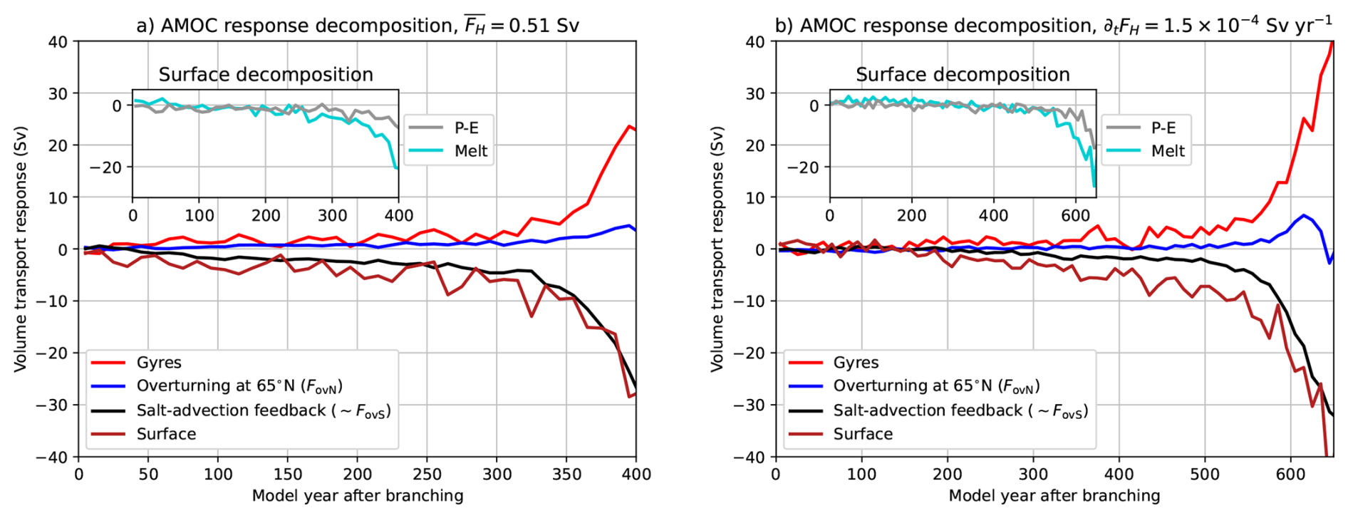
Figure 4 (a, b) Decomposition of the AMOC feedbacks (Vanderborght et al., 2025) for the (a) $\stackrel{\mathrm{‾}}{F_H}=\mathrm{0.51}$ Sv simulation (i.e., red curve in panel 2h) and the (a) half-rate forcing simulation ($\mathrm{1.5}\times {\mathrm{10}}^{-\mathrm{4}}$ Sv yr⁻¹). The inset shows the two surface components of Arctic sea-ice melt and precipitation minus evaporation (P−E). The time series are presented as 10-year averages (to reduce the variance). Note the different horizontal ranges between the two panels.

First the $\stackrel{\mathrm{‾}}{F_H}=\mathrm{0.51}$ Sv simulation (Fig. 4a), in which the AMOC weakens by about 1.5 Sv during the first 100 model years. This weakening is attributed to the slightly larger freshwater forcing (+0.015 Sv) compared to the starting equilibrium solution at $\stackrel{\mathrm{‾}}{F_H}=\mathrm{0.495}$ Sv. The destabilizing salt-advection feedback (linked to F_ovS) and surface (mainly sea-ice melt) feedback slowly grow over the following 250 years. Over the same period (model years 100–350), the gyres and overturning component at 65° N partly stabilize the AMOC. The combined effect results in an AMOC weakening of only 1.5 Sv over these 250 years and after model year 350 the AMOC fully collapses. The salt-advection feedback eventually becomes dominant and this destabilising feedback fully develops over centennial timescales (under constant freshwater flux forcing).

Next the half-rate forcing simulation (Fig. 4b), where we find a similar centennial timescale for the destabilizing AMOC feedbacks. The AMOC feedbacks remain relatively small up to model year 350 (F_H=0.503 Sv), then slowly increase in the following 200 years (model years 350–550) and thereafter the AMOC fully collapses. This gradual increase of the destabilizing feedbacks between model year 350 to 500, suggests that the AMOC will eventually tip and hence branching simulations with fixed F_H for F_H≥0.503 Sv will also result in an AMOC collapse, similarly as the standard quasi-equilibrium simulation. However, additional simulations are needed to find this critical value, which were not done here.

In other words, there is a certain critical value of forcing and, once crossed, the AMOC will eventually tip over centennial timescales (≈200 model years). This critical value is dependent on the initial condition and rate of forcing, which we will make more explicit with the E-CCM below. As argued above, for the half-forcing quasi-equilibrium simulation this critical value is likely around F_H=0.503 Sv, which is well within the interval 0.495 Sv $\le \stackrel{\mathrm{‾}}{F_H}<$ 0.51 Sv. The AMOC collapse starts at F_H=0.525 Sv in the standard quasi-equilibrium simulation, meaning that the destabilizing feedbacks were growing during the 200 model years (ΔF_H=0.06 Sv) prior to the collapse (Vanderborght et al., 2025). This suggests that $\stackrel{\mathrm{‾}}{F_H}=\mathrm{0.525}-\mathrm{0.06}=\mathrm{0.465}$ Sv is the latest statistical equilibrium which can be found when directly branching from the quasi-equilibrium simulation, which is indeed the case here (Fig. 2e, k). This confirms again that the standard quasi-equilibrium simulation undershoots the upper bound of the multi-stable regime. The implication is that an overshooting (or undershooting) AMOC cannot be assessed by only analysing the onset of the AMOC tipping event. In fact, the onset of the AMOC tipping event only indicates where the destabilising feedbacks become dominant and it is much more useful to analyse the changes in AMOC feedback strengths.

What is important here, is that the half-rate forcing's transition to the collapsed state is twice as fast (in F_H space), which is a typical characteristic of transitions near a saddle-node bifurcation (Berglund and Gentz, 2006) (see also Appendix B). The duration of AMOC transitions in both quasi-equilibria and in the statistical equilibrium simulations (Fig. 2) is about 100 years and the full equilibration to the collapsed AMOC state requires more than 500 years (van Westen et al., 2024a). Another characteristic of a saddle-node bifurcation is the loss of resilience (i.e., critical slow down) near the tipping point (van Westen et al., 2024b). This can be quantified by determining the variance and (lag-1) autocorrelation of specific observables. For the AMOC strength, we find no indications of critical slow down (not shown) which is consistent with the results in van Westen et al. (2024a). There is also no increase in the variance for the AMOC strength for both the quasi-equilibria and the statistical equilibria (Fig. 3c). However, for the physics-based quantity F_ovS we find indications of critical slowdown (van Westen et al., 2024a; Smolders et al., 2025). Indeed, the F_ovS variance increases for larger F_H up to the tipping event (Fig. 3d). This increase in variability indicates that the AMOC loses resilience and makes it more prone to transitions.

3.2 Equilibria in the E-CCM

The AMOC behaviour in the CESM can be reproduced with the E-CCM under varying freshwater flux forcing (now E_A). For the E-CCM, the steady states obtained using continuation techniques (cf. Sect. 2.2) are presented in Fig. 5a, b for the AMOC strength and F_ovS, respectively. The continuation indicates two saddle-node bifurcations at $E_{\mathrm{A}}^{\mathrm{1}}=\mathrm{0.4861}$ Sv (AMOC on) and at $E_{\mathrm{A}}^{\mathrm{2}}=\mathrm{0.1857}$ Sv (AMOC off). The AMOC on and unstable steady states clearly show the square-root behaviour between AMOC strength and E_A, which arises from the dominant salt-advection feedback close to $E_{\mathrm{A}}^{\mathrm{1}}$. The probabilities under (stochastic) noise for the transition from an AMOC on to an AMOC off state approach 1 when moving closer to $E_{\mathrm{A}}^{\mathrm{1}}$ (van Westen et al., 2024b), indicative of the loss of resilience. Here, we performed deterministic quasi-equilibrium and equilibrium simulations with the E-CCM, which are shown in Fig. 5. Note that we used slightly different freshwater flux forcing (E_A) values in the E-CCM than in the CESM.

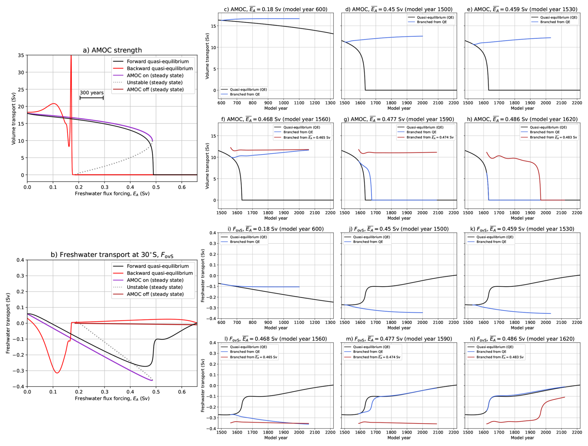
Figure 5 Similar to Fig. 2, but now for the E-CCM. Note that in panels (a) and (b) the steady and unstable states (from the continuation) are also shown.

The quasi-equilibrium hysteresis simulation in the E-CCM is (qualitatively) comparable to that of the CESM (compare Figs. 2 and 5); the large overshoot (>35 Sv) in the E-CCM upon AMOC recovery is a model artefact (van Westen et al., 2024b). In the forward quasi-equilibrium simulation the AMOC strength is lower compared to the value at the steady states, while the F_ovS values are higher. The branches from the quasi-equilibrium eventually collapse for $\stackrel{\mathrm{‾}}{E_{\mathrm{A}}}=\mathrm{0.477}$ Sv and $\stackrel{\mathrm{‾}}{E_{\mathrm{A}}}=\mathrm{0.486}$ Sv, meaning that a critical $\stackrel{\mathrm{‾}}{E_{\mathrm{A}}}$ value was surpassed, which is then also the case for the quasi-equilibrium simulation.

In contrast to the CESM, it is computationally feasible to quantify this critical value in the E-CCM. Here, we define the critical branch as the branch from the quasi-equilibrium that collapses at the lowest possible $\stackrel{\mathrm{‾}}{E_{\mathrm{A}}}$ value. We use an accuracy of $\mathrm{\Delta }\stackrel{\mathrm{‾}}{E_{\mathrm{A}}}=\mathrm{0.001}$ Sv (but can be even higher when needed). Ultimately, the AMOC collapses when branching from the quasi-equilibrium simulation for $\stackrel{\mathrm{‾}}{E_{\mathrm{A}}}\ge \mathrm{0.474}$ Sv (Fig. 6a). As was argued in the previous section, this critical value is also dependent on the initial condition and rate of forcing. For example, when we use the steady state at $\stackrel{\mathrm{‾}}{E_{\mathrm{A}}}=\mathrm{0.45}$ Sv as initial condition, we can increase E_A up to 0.479 Sv (with $\mathrm{3}\times {\mathrm{10}}^{-\mathrm{4}}$ Sv yr⁻¹) and then keeping the freshwater flux forcing constant. In this case, the AMOC eventually equilibrates to the AMOC on state (not shown), meaning that the critical value is found for $\stackrel{\mathrm{‾}}{E_{\mathrm{A}}}\ge \mathrm{0.480}$ Sv. When we initiate from E_A=0 Sv while using a ten times smaller forcing rate ($\mathrm{3}\times {\mathrm{10}}^{-\mathrm{5}}$ Sv yr⁻¹), the AMOC also equilibrates to the AMOC on state when increasing E_A up to 0.483 Sv and then keeping the freshwater flux forcing constant (not shown). The critical value for this other case is for $\stackrel{\mathrm{‾}}{E_{\mathrm{A}}}\ge \mathrm{0.484}$ Sv. Depending on the initialisation and forcing rate, the saddle-node bifurcation can only be reached with a limited accuracy.

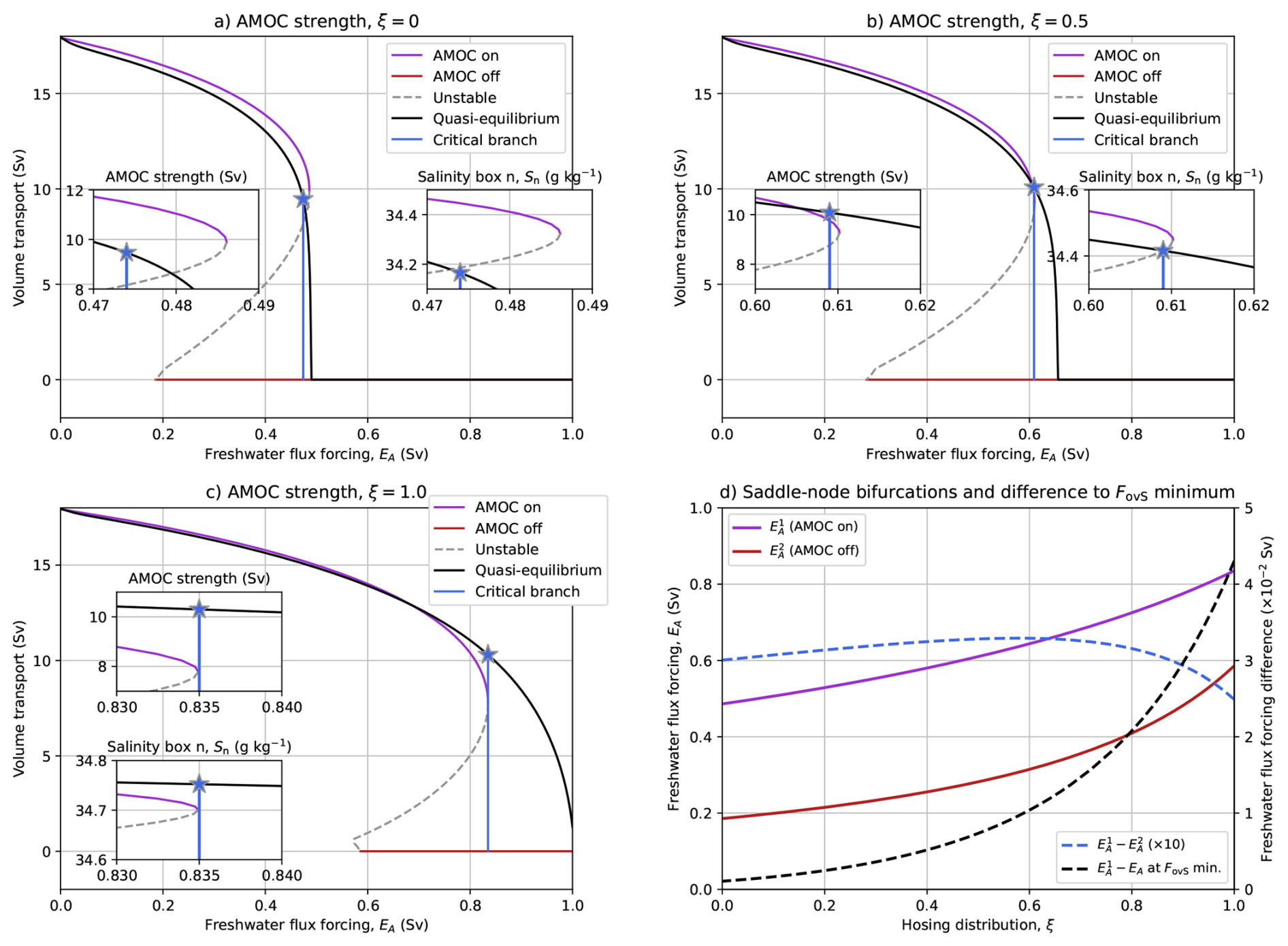
Figure 6 (a) The steady states for the AMOC strength and a quasi-equilibrium simulation (rate $\mathrm{3}\times {\mathrm{10}}^{-\mathrm{4}}$ Sv yr⁻¹) for the hosing over box n (ξ=0). A simulation was branched from the quasi-equilibrium simulation for $\stackrel{\mathrm{‾}}{E_{\mathrm{A}}}=\mathrm{0.474}$ Sv (blue star), which was integrated into equilibrium. The two insets show zoomed-in versions of the AMOC strength and salinity of box n near the saddle-node bifurcation. (b, c) Similar to panel a, but now for (b) ξ=0.5 and (c) ξ=1, where the branched simulations were initiated at $\stackrel{\mathrm{‾}}{E_{\mathrm{A}}}=\mathrm{0.609}$ Sv and $\stackrel{\mathrm{‾}}{E_{\mathrm{A}}}=\mathrm{0.835}$ Sv, respectively. (d) The position of the saddle-node bifurcations of the AMOC on ($E_{\mathrm{A}}^{\mathrm{1}}$) and AMOC off ($E_{\mathrm{A}}^{\mathrm{2}}$) states (solid curves). The distance (expressed in ΔE_A) between $E_{\mathrm{A}}^{\mathrm{1}}$ and $E_{\mathrm{A}}^{\mathrm{2}}$ and between the $E_{\mathrm{A}}^{\mathrm{1}}$ and the F_ovS minimum.

Since the AMOC collapses at critical values lower than (i.e., undershooting) the saddle-node bifurcation (blue curve in Fig. 6a), the system must cross the basin boundary of attraction between the AMOC on and AMOC off states. The continuation allows us to explore which variable (temperature, salinity, and pycnocline depth), or which specific combination of variables (e.g., AMOC strength, see Eq. 1), crosses this boundary of attraction. Notably, the critical branch at $\stackrel{\mathrm{‾}}{E_{\mathrm{A}}}=\mathrm{0.474}$ Sv does not cross the basin boundary with respect to AMOC strength and one expects AMOC recovery to the AMOC on state, and yet the AMOC collapses (left inset in Fig. 6a). This means that the AMOC strength is no good predictor for the future evolution of the system for the critical branch. When we analyse a different quantity, such as the salinity of box n (right inset in Fig. 6a), it does cross the basin boundary. The salinity in box n is important here as it (partly) sets the AMOC strength (relation 1) and is influenced under the destabilizing salt-advection feedback, which gives rise to the quadratic relation between AMOC strength and freshwater flux forcing.

When we equally distribute the hosing over box n and box t (ξ=0.5, Fig. 6b), the saddle-node bifurcations shift to higher values of E_A. The quasi-equilibrium for this case has weaker AMOC strengths than the stable AMOC on state and close to the saddle-node bifurcation it has stronger strengths than the AMOC on state (left inset in Fig. 6b). The critical branch (at $\stackrel{\mathrm{‾}}{E_{\mathrm{A}}}=\mathrm{0.609}$ Sv) has a stronger AMOC strength than the steady AMOC on state upon branching, but it still collapses. The salinity in box n does cross the basin boundary (right inset in Fig. 6b), demonstrating again that AMOC strength is no good indicator for predicting the future AMOC trajectory. Only when the hosing is applied over box t (ξ=1.0, Fig. 6c), the AMOC collapses when increasing the freshwater flux forcing beyond the saddle-node bifurcation of $E_{\mathrm{A}}^{\mathrm{1}}=\mathrm{0.83495}$ Sv. When we branch from the quasi-equilibrium for lower E_A than the saddle-node bifurcation (e.g., $\stackrel{\mathrm{‾}}{E_{\mathrm{A}}}=\mathrm{0.8348}$ Sv, not shown), the solution equilibrates to the stable AMOC on state.

The AMOC dynamics and the under- and overshooting behaviour can be understood from these three different cases. When a hosing perturbation is (partly) applied over box n, the AMOC strength directly reduces as the meridional salinity difference between box n and box ts increases. The largest part of the freshwater perturbation is carried away by the AMOC to box d, but a small part of the perturbation remains in box n (due to a weaker AMOC) and causes freshwater accumulation over box n. This freshwater accumulation results in a slightly weaker AMOC strengths compared to the steady states. Once the system has a sufficient amount of time to adjust to the imposed freshwater perturbation, the entire freshwater perturbation is redistributed over the boxes and the AMOC strength eventually increases (e.g., blue curves in Fig. 5c, d, e, f). In other words, the advective (“flushing”) timescale is slower than the hosing timescale, resulting in an enhanced AMOC strength decline. This makes the AMOC more prone to freshwater perturbations and explains why there is hardly any overshoot in the quasi-equilibrium simulation with the saddle-node bifurcation (for ξ=0). This is qualitatively different than the quasi-equilibrium CESM, meaning that ξ=0 is not very likely for the CESM.

The direct AMOC weakening effect is smaller when adding (part of) the hosing over box t and there are two effects contributing to this different behaviour. First, the hosing is now distributed over the (much) larger box t than box n and making the salinity anomalies (averaged over box t) effectively smaller. Second, only a part of the salinity perturbations from box t is carried by the AMOC into box n and most of it is directly carried to box d (see also Fig. 1). This implies that the role of the overturning contribution in redistributing salinity anomalies between box t and box n is getting smaller, while the (northern) gyre contribution is getting more important. These combined effects explain why the saddle-node bifurcations shift to larger E_A values for increasing ξ (Fig. 6d). The larger gyre contribution is also reflected in a greater ΔE_A between the $E_{\mathrm{A}}^{\mathrm{1}}$ and F_ovS minimum, which also modifies the hysteresis width which is measured as the distance between the two saddle-node bifurcations (Fig. 6d).

In the standard quasi-equilibrium CESM simulation (rate $\mathrm{3}\times {\mathrm{10}}^{-\mathrm{4}}$ Sv yr⁻¹), the AMOC strength is also smaller than that of the statistical equilibria. Thereafter, the AMOC appears to overshoot the upper bound of the multi-stable regime. The CESM trajectory shares similar characteristics as the E-CCM in the ξ=0.5 configuration, which is consistent with the applied hosing region in the CESM (20° N–50° N), though the CESM is much more complex than the E-CCM. Depending on the hosing region, one can change the relative contributions of important AMOC feedbacks and this results in differences in AMOC sensitivity, the onset of the AMOC tipping event and width of the multi-stable regime. It is therefore important to use a fixed hosing region, as was done for our CESM simulations or in the outlined procedure of the North Atlantic Hosing Model Intercomparison Project (NAHosMIP, Jackson et al., 2023). Sensitivity experiments indicate that the northern portion of the North Atlantic (e.g., the Irminger basin) is most sensitive under hosing (Rahmstorf, 1996; Ma et al., 2024). Nevertheless, the destabilising salt-advection feedback becomes more dominant under increasing hosing strengths and causes the square-root dependency near the saddle-node bifurcation.

4 Feedback analysis in the CESM

The results from Sect. 3.2 demonstrate that as long as the salt-advection feedback dominates, one may expect a square root dependence in the AMOC on state under increasing freshwater flux forcing, similar to the Stommel model (see Appendix A). Although the AMOC is (highly) idealised in the E-CCM, it is qualitatively able to reproduce almost all AMOC characteristics of that in a much more complex and fully-coupled climate model (i.e., the CESM). This makes the existence of a saddle-node bifurcation in the CESM plausible, but this can not easily be demonstrated using only a limited number of equilibrium simulations. However, it turns out that from performing a feedback analysis as in Vanderborght et al. (2025), we can (under reasonable assumptions) derive a reduced model explicitly showing the dependence of AMOC strength on F_H.

4.1 Reduced model derivation

We start from the total Atlantic (34° S to 65° N) freshwater budget as governed by (Vanderborght et al., 2025):

$$\begin{array}{}\text{(2)}& {\displaystyle \frac{\mathrm{d}W}{\mathrm{d}t}}=F_{\mathrm{azS}}-F_{\mathrm{azN}}+F_{\mathrm{ovS}}-F_{\mathrm{ovN}}+F_{\mathrm{surf}}+F_{\mathrm{res}},\end{array}$$

where W is the total freshwater content. The Atlantic freshwater content can be modified through azonal (gyre) contributions (i.e., F_azS and F_azN), overturning contributions (i.e., F_ovS and F_ovN), surface contribution (i.e., F_surf) and residual contribution (i.e., F_res). The quantities F_azS and F_ovS are evaluated at 34° S, hence indicated with subscript “S”, and we follow a similar notation for the northern boundary (65° N) by using a subscript “N”.

Upon a freshwater perturbation, the evolution of the different contributions depends on the background state and the AMOC strength (Vanderborght et al., 2025). The AMOC strength is fairly homogeneous over the Atlantic basin (van Westen et al., 2024a) and we assume a northward volume transport in the upper AMOC limb which we indicate here as Ψ; the lower AMOC limb then carries Ψ southward. The velocity-weighted average salinity over the upper AMOC limb is indicated with S_→, and similarly for the lower AMOC limb we use S_←. The vertical salinity difference between the upper AMOC limb and lower AMOC limb is then indicated by $S_{\rightleftarrows }=S_{\to }-S_{\leftarrow }$. Under this idealization it directly follows that:

$$\begin{array}{}\text{(3)}& F_{\mathrm{ovS}}=-{\displaystyle \frac{S_{\rightleftarrows }}{S_{\mathrm{0}}}}\mathrm{\Psi },\end{array}$$

where S₀=35 g kg⁻¹. Because the salinity transport in the lower AMOC limb is approximately adiabatic, the vertical salinity contrast at 34° S is closely related to a meridional salinity contrast between 34° S and the North Atlantic sinking region. This meridional salinity contrast is related to the AMOC strength via thermal wind balance (Butler et al., 2016). Therefore, the vertical salinity contrast scales with the AMOC strength as (Vanderborght et al., 2025):

$$\begin{array}{}\text{(4)}& \mathrm{\Psi }={\mathrm{\Psi }}_{\mathrm{0}}+c_{\mathrm{2}}\left(\mathrm{1}-c_{\mathrm{1}}\right)\left(S_{\rightleftarrows }\left(\mathrm{0}\right)-S_{\rightleftarrows }\right),\end{array}$$

where c₁ represents the stabilizing thermal-advective feedback and c₂ is a scaling factor. Both c₁ and c₂ are positive constants and, for the CESM, their values are about 0.52 and 20 Sv kg g⁻¹ (Vanderborght et al., 2025). The terms Ψ₀ and S_⇄(0) are the AMOC strength and vertical salinity difference for F_H=0 Sv (no hosing), respectively.

Under the applied hosing (indicated by δF_H in the CESM) the value of F_surf increases and is primarily (i.e., to first order) balanced by a declining F_ovS (van Westen et al., 2024a). On the other hand, the gyres flush freshwater anomalies out of the Atlantic Ocean and stabilize the AMOC (Vanderborght et al., 2025). Sijp (2012) argued that S_⇄ linearly scales with the integrated Atlantic freshwater content. This integrated freshwater content in turn scales with the anomalous freshwater transport by the gyres (Huisman et al., 2010), i.e.:

$$\begin{array}{}\text{(5)}& F_{\mathrm{gyre}}=F_{\mathrm{azS}}-F_{\mathrm{azN}}=-g_{\mathrm{1}}{S}_{\rightleftarrows }+g_{\mathrm{2}}.\end{array}$$

This linear relation is also applicable for the CESM, where g₁=0.032 Sv kg g⁻¹ and g₂=0.49 Sv (Fig. 7a). The last contribution which we consider is the overturning component at the northern boundary, F_ovN. The AMOC strength almost vanishes at the northern boundary and the expression for F_ovN is different than that of the F_ovs (relation 3). The F_ovN scales linearly with S_⇄ and can be approximated by:

$$\begin{array}{}\text{(6)}& F_{\mathrm{ovN}}=n_{\mathrm{1}}{S}_{\rightleftarrows }+n_{\mathrm{2}}\end{array}$$

with n₁=0.025 Sv kg g⁻¹ and $n_{\mathrm{2}}=-\mathrm{0.021}$ Sv for the CESM as shown in Fig. 7b. The contributions by the gyres and F_ovN scale linearly with increasing S_⇄ (or decreasing Ψ), whereas the F_ovS has a non-linear contribution. To be more precise, the F_ovS is determined by the product of the vertical salinity difference and the AMOC strength, where the latter scales linearly with the vertical salinity difference (i.e., relation 4). The F_ovS scales quadratically with AMOC strength, and conversely AMOC strength scales with the square root dependence on F_ovS. As the imposed freshwater flux forcing is primarily balance by F_ovS in the CESM (van Westen et al., 2024a), one expects a square root dependence in AMOC strength under increasing freshwater flux forcing.

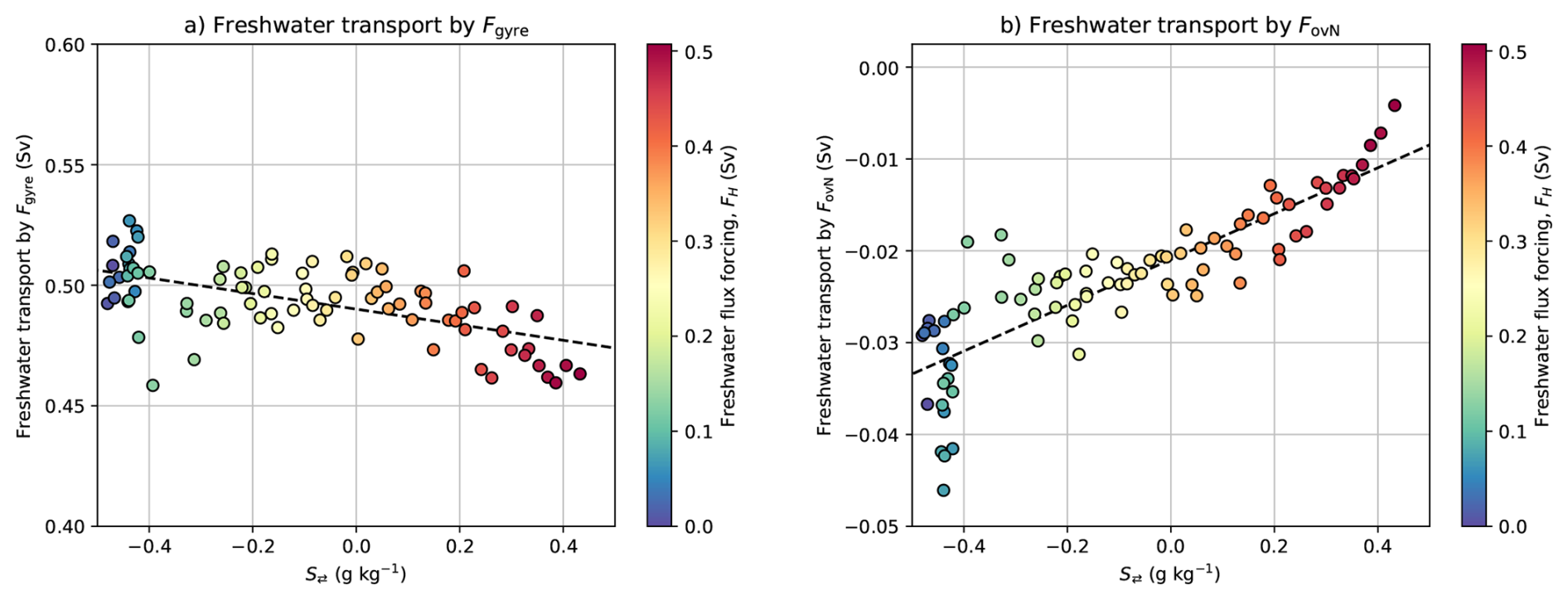
Figure 7 (a) The relation between F_gyre and S_⇄, where the linear fit is determined over the 20-year averages up to model year 1700 (F_H=0.51 Sv) of the standard quasi-equilibrium simulation. (b) Similar to panel a, but now for the F_ovN and S_⇄.

A perturbation in the Atlantic freshwater content (cf. 2) around an equilibrium state then gives:

$$\begin{array}{}\text{(7)}& -\mathit{\delta }{F}_{\mathrm{ovS}}+\mathit{\delta }{F}_{\mathrm{ovN}}-\mathit{\delta }{F}_{\mathrm{gyre}}=\mathit{\delta }{F}_{\mathrm{surf}},\end{array}$$

and using the expressions for F_ovS, F_gyre and F_ovN, this yields:

$$\begin{array}{}\text{(8)}& \mathrm{\Psi }\mathit{\delta }{S}_{\rightleftarrows }+S_{\rightleftarrows }\mathit{\delta }\mathrm{\Psi }+n_{\mathrm{1}}{S}_{\mathrm{0}}\mathit{\delta }{S}_{\rightleftarrows }+g_{\mathrm{1}}{S}_{\mathrm{0}}\mathit{\delta }{S}_{\rightleftarrows }=S_{\mathrm{0}}\mathit{\delta }{F}_H\end{array}$$

Using the relation between Ψ and S_⇄ (from 4) we find:

$$\begin{array}{}\text{(9)}& \begin{array}{rl}-{\displaystyle \frac{\mathrm{\Psi }}{c_{\mathrm{2}}(\mathrm{1}-c_{\mathrm{1}})}}\mathit{\delta }\mathrm{\Psi }& +(-{\displaystyle \frac{\mathrm{\Psi }}{c_{\mathrm{2}}(\mathrm{1}-c_{\mathrm{1}})}}+{\displaystyle \frac{{\mathrm{\Psi }}_{\mathrm{0}}}{c_{\mathrm{2}}(\mathrm{1}-c_{\mathrm{1}})}}\\ & +S_{\rightleftarrows }\left(\mathrm{0}\right)-{\displaystyle \frac{(n_{\mathrm{1}}+g_{\mathrm{1}})S_{\mathrm{0}}}{c_{\mathrm{2}}(\mathrm{1}-c_{\mathrm{1}})}})\mathit{\delta }\mathrm{\Psi }\\ & =S_{\mathrm{0}}\mathit{\delta }{F}_H,\end{array}\end{array}$$

which can be rewritten as:

$$\begin{array}{}\text{(10)}& \begin{array}{rl}(-\mathrm{2}\mathrm{\Psi }& +{\mathrm{\Psi }}_{\mathrm{0}}+c_{\mathrm{2}}(\mathrm{1}-c_{\mathrm{1}})S_{\rightleftarrows }\left(\mathrm{0}\right)-(n_{\mathrm{1}}+g_{\mathrm{1}})S_{\mathrm{0}})\mathit{\delta }\mathrm{\Psi }\\ & =c_{\mathrm{2}}(\mathrm{1}-c_{\mathrm{1}})S_{\mathrm{0}}\mathit{\delta }{F}_H,\end{array}\end{array}$$

and integrating both sides gives:

$$\begin{array}{}\text{(11)}& \begin{array}{rl}{\mathrm{\Psi }}^{\mathrm{2}}& -({\mathrm{\Psi }}_{\mathrm{0}}+c_{\mathrm{2}}(\mathrm{1}-c_{\mathrm{1}}\left)S_{\rightleftarrows }\right(\mathrm{0})-(n_{\mathrm{1}}+g_{\mathrm{1}}\left)S_{\mathrm{0}}\right)\mathrm{\Psi }\\ & +c_{\mathrm{2}}(\mathrm{1}-c_{\mathrm{1}})S_{\mathrm{0}}{F}_H+C=\mathrm{0},\end{array}\end{array}$$

with integration constant C. The solution with $\mathrm{\Psi }(F_H=\mathrm{0})={\mathrm{\Psi }}_{\mathrm{0}}$ is:

$$\begin{array}{}\text{(12)}& \begin{array}{rl}\mathrm{\Psi }\left(F_H\right)& ={\displaystyle \frac{{\mathrm{\Psi }}_{\mathrm{0}}}{\mathrm{2}}}+{\displaystyle \frac{c_{\mathrm{2}}(\mathrm{1}-c_{\mathrm{1}})S_{\rightleftarrows }\left(\mathrm{0}\right)}{\mathrm{2}}}-{\displaystyle \frac{(n_{\mathrm{1}}+g_{\mathrm{1}})S_{\mathrm{0}}}{\mathrm{2}}}\\ & \pm \sqrt{{\left({\displaystyle \frac{\begin{array}{c}{\mathrm{\Psi }}_{\mathrm{0}}-c_{\mathrm{2}}(\mathrm{1}-c_{\mathrm{1}})S_{\rightleftarrows }\left(\mathrm{0}\right)\\ +(n_{\mathrm{1}}+g_{\mathrm{1}})S_{\mathrm{0}}\end{array}}{\mathrm{2}}}\right)}^{\mathrm{2}}-c_{\mathrm{2}}(\mathrm{1}-c_{\mathrm{1}})S_{\mathrm{0}}{F}_H}\end{array}\end{array}$$

Rather using S_⇄(0), we express it as the initial F_ovS using Eq. (3), i.e., $S_{\rightleftarrows }\left(\mathrm{0}\right)=-\frac{S_{\mathrm{0}}{F}_{\mathrm{ovS}}\left(\mathrm{0}\right)}{{\mathrm{\Psi }}_{\mathrm{0}}}$. The final expression becomes:

$$\begin{array}{}\text{(13)}& \begin{array}{rl}\mathrm{\Psi }\left(F_H\right)& ={\displaystyle \frac{{\mathrm{\Psi }}_{\mathrm{0}}}{\mathrm{2}}}-{\displaystyle \frac{c_{\mathrm{2}}\left(\mathrm{1}-c_{\mathrm{1}}\right)S_{\mathrm{0}}{F}_{\mathrm{ovS}}\left(\mathrm{0}\right)}{\mathrm{2}{\mathrm{\Psi }}_{\mathrm{0}}}}-{\displaystyle \frac{(n_{\mathrm{1}}+g_{\mathrm{1}})S_{\mathrm{0}}}{\mathrm{2}}}\\ & \pm \sqrt{{\left({\displaystyle \frac{\begin{array}{c}{\mathrm{\Psi }}_{\mathrm{0}}^{\mathrm{2}}+c_{\mathrm{2}}\left(\mathrm{1}-c_{\mathrm{1}}\right)S_{\mathrm{0}}{F}_{\mathrm{ovS}}\left(\mathrm{0}\right)\\ +(n_{\mathrm{1}}+g_{\mathrm{1}})S_{\mathrm{0}}{\mathrm{\Psi }}_{\mathrm{0}}\end{array}}{\mathrm{2}{\mathrm{\Psi }}_{\mathrm{0}}}}\right)}^{\mathrm{2}}-c_{\mathrm{2}}\left(\mathrm{1}-c_{\mathrm{1}}\right)S_{\mathrm{0}}{F}_H}\end{array}\end{array}$$

Do note that several assumptions are required to arrive at this final expression. For example, various residual (F_res) and climate feedbacks were not considered, such as ocean-sea ice interactions (destabilizing), ocean-atmosphere fluxes (destabilizing), pycnocline deepening (stabilising), open Bering strait (stabilizing) and the effect of ocean eddies (stabilizing) (Vanderborght et al., 2025). The linear relation in F_gyre and F_ovN with S_⇄ is less accurate and c₁ is less constant close to the tipping point. Freshwater anomalies may be stored in the Atlantic Ocean and hence we assumed that changes in the freshwater content are much smaller than changes in the freshwater balance terms (i.e., $\frac{\mathrm{d}W}{\mathrm{d}t}\ll \mathrm{\Delta }\left(F_{\mathrm{azS}}-F_{\mathrm{azN}}+F_{\mathrm{ovS}}-F_{\mathrm{ovN}}+F_{\mathrm{surf}}+F_{\mathrm{res}}\right)$). These additional feedbacks and processes modify the idealized AMOC response and make it more difficult to derive an analytical solution for the northward overturning regime, as these processes (ideally) need to be expressed as a function of S_⇄ (if it exists). We stress that this idealized AMOC response under hosing should be interpreted with care and one needs to consider the appropriate feedback contributions for each (climate) model set-up. The key point is that the AMOC strength exhibits a square-root dependence on the freshwater flux forcing, leading to a saddle-node bifurcation when the dominant balance is between the applied freshwater flux forcing and the overturning component. As long as other contributions remain sufficiently small, their effect will not change the structure (and therefore the type) of the bifurcation diagram. Indeed, the F_gyre and F_ovN remain fairly linear up to F_H=0.51 Sv (Fig. 7) and this is beyond the critical forcing (0.465 Sv$<\stackrel{\mathrm{‾}}{F_H}\le$ 0.48 Sv, Fig. 2) for which the salt-advection feedback becomes dominant. Once the AMOC starts to collapse, the different AMOC contributions become much larger (e.g., Fig. 4) and their responses are attributed to large-scale adjustments under a collapsing AMOC.

For the Stommel 2-box model, we can demonstrate that a similar AMOC response holds (see Appendix A). Under no freshwater flux forcing (η=0) in this model, the salinity difference between the two boxes is zero. This constraint gives the initial AMOC strength of Ψ₀=kαΔT^a and $F_{\mathrm{ovS}}(\mathit{\eta }=\mathrm{0})=\mathrm{0}$, where k is a hydraulic pumping coefficient, α the (dimensionless) thermal expansion coefficient, and ΔT^a the (dimensionless) atmospheric temperature difference. The northern boundary is closed (n₁=0) and gyres are not represented (g₁=0) in the Stommel model. The oceanic temperatures in the Stommel model are fixed (under steady state assumption), and in this case c₁=0. Relation (13) for the Stommel model reduces to:

$$\begin{array}{}\text{(14)}& \mathrm{\Psi }\left(F_H\right)={\displaystyle \frac{k\mathit{\alpha }\mathrm{\Delta }{T}^{\mathrm{a}}}{\mathrm{2}}}\pm \sqrt{{\left({\displaystyle \frac{k\mathit{\alpha }\mathrm{\Delta }{T}^{\mathrm{a}}}{\mathrm{2}}}\right)}^{\mathrm{2}}-c_{\mathrm{2}}{S}_{\mathrm{0}}{F}_H}\end{array}$$

and is similar to relation (A9), apart from some scaling coefficients.

4.2 Application of the reduced model

Using the reduced model, the critical value of F_H for an AMOC collapse in the CESM can be estimated by assuming that the freshwater flux forcing is (in its first order) balanced by the overturning and azonal (gyre) components, which is the case for the CESM (van Westen et al., 2024a). The critical freshwater flux forcing is obtained by setting the terms under the square root in Eq. (13) equal to zero. Solving this yields:

$$\begin{array}{}\text{(15)}& F_H^{\mathrm{c}}={\displaystyle \frac{\mathrm{1}}{c_{\mathrm{2}}\left(\mathrm{1}-c_{\mathrm{1}}\right)S_{\mathrm{0}}}}{\left({\displaystyle \frac{\begin{array}{c}{\mathrm{\Psi }}_{\mathrm{0}}^{\mathrm{2}}+c_{\mathrm{2}}\left(\mathrm{1}-c_{\mathrm{1}}\right)S_{\mathrm{0}}{F}_{\mathrm{ovS}}\left(\mathrm{0}\right)\\ +(n_{\mathrm{1}}+g_{\mathrm{1}})S_{\mathrm{0}}{\mathrm{\Psi }}_{\mathrm{0}}\end{array}}{\mathrm{2}{\mathrm{\Psi }}_{\mathrm{0}}}}\right)}^{\mathrm{2}}.\end{array}$$

The $F_H^{\mathrm{c}}$ is dependent on the initial AMOC strength and initial F_ovS value. In the CESM, the Atlantic Ocean surface area outside 20–50° N receives a negative freshwater flux as part of the global compensation (see inset Fig. 2a). This makes the applied hosing 86 % effective when considering the total Atlantic Ocean surface area (34° S–65° N) and $F_H^{\mathrm{c}}$ needs to be adjusted by a factor $\frac{\mathrm{1}}{\mathrm{0.86}}$. The time-means (first 50 model years) in the CESM quasi-equilibrium simulation are Ψ₀=16 Sv and F_ovS(0)=0.22 Sv, which give: $F_H^{\mathrm{c}}=\frac{\mathrm{1}}{\mathrm{0.86}}\mathrm{0.38}=\mathrm{0.44}$ Sv (Fig. 8a, b). When using the maximum and minimum values (over the first 50 model years) for AMOC strength and F_ovS, we find $F_H^{\mathrm{c}}=\frac{\mathrm{1}}{\mathrm{0.86}}\mathrm{0.44}=\mathrm{0.52}$ Sv and $F_H^{\mathrm{c}}=\frac{\mathrm{1}}{\mathrm{0.86}}\mathrm{0.33}=\mathrm{0.38}$ Sv, respectively (Fig. 8a, b).

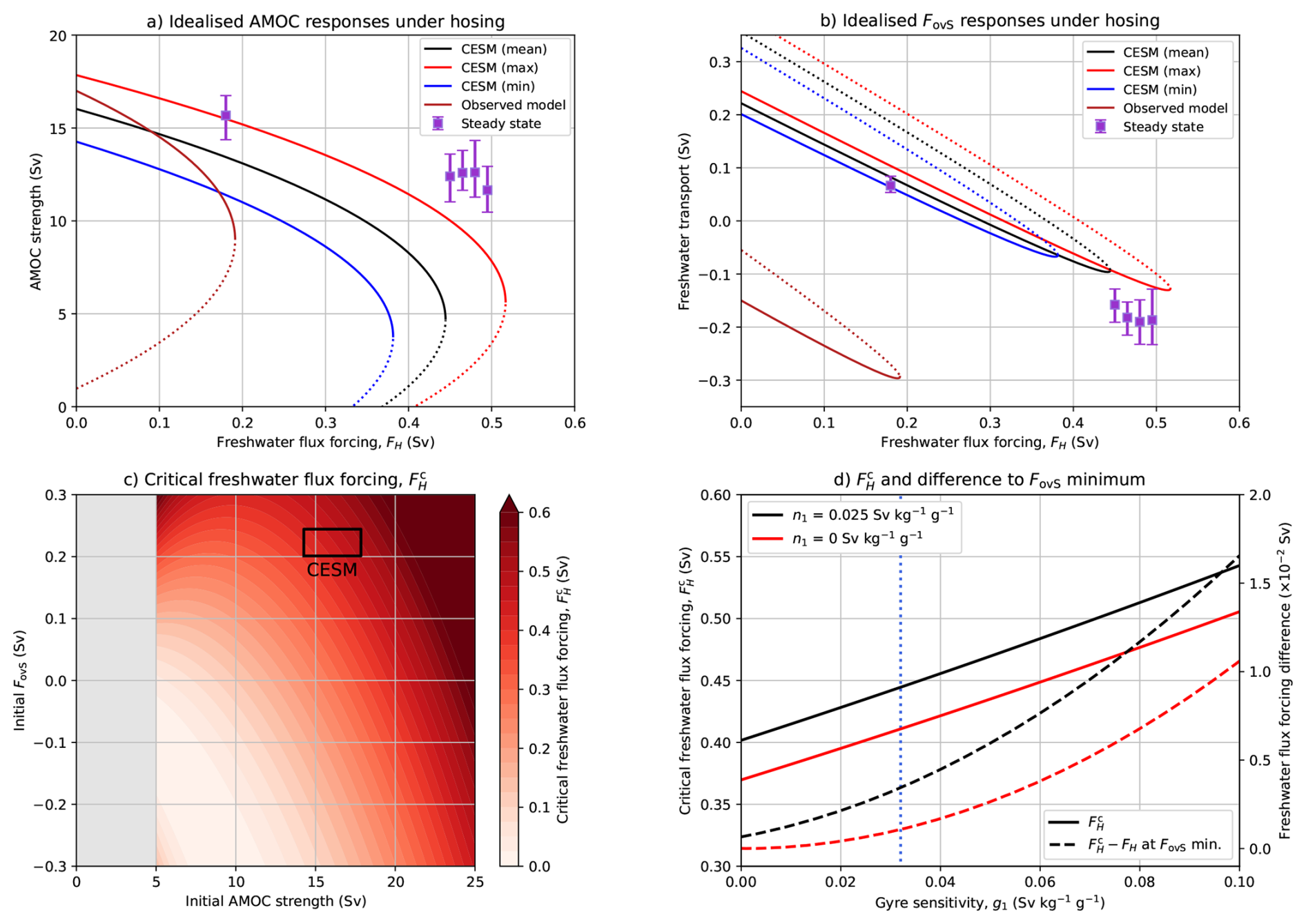
Figure 8 (a, b) The AMOC and F_ovS responses of the reduced model under the freshwater flux forcing (cf. Eqs. 13 and 3, respectively), where the solid curves indicate the steady AMOC on state and dotted curves the unstable branch. The initial values for both the AMOC strength and F_ovS were obtained from the first 50 model years of the quasi-equilibrium. The AMOC strength values are 16.0 Sv (mean), 17.8 Sv (maximum) and 14.3 Sv (minimum), and F_ovS values are 0.22 Sv (mean), 0.24 Sv (maximum) and 0.20 Sv (minimum). For the “Observed model”, we use the reduced model in combination with observed values of 17 Sv (Smeed et al., 2018) and −0.15 Sv (Arumí-Planas et al., 2024) for the AMOC strength and F_ovS, respectively. (c) The critical freshwater flux forcing ($F_H^{\mathrm{c}}$) for varying initial AMOC strength and initial F_ovS. The ranges for the CESM (first 50 model years of quasi-equilibrium) are indicated. The critical freshwater flux forcing was not determined for relatively weak AMOC strengths (<5 Sv). (d) Values of $F_H^{\mathrm{c}}$ (solid curves) and difference to F_ovS minimum (dashed curves) for varying gyre sensitivity (g₁) and two cases for the northern overturning sensitivity (n₁), using the time-mean (first 50 model years) AMOC strength and F_ovS. The standard CESM values are g₁=0.032 Sv kg g⁻¹ (blue dotted line) and n₁=0.025 Sv kg g⁻¹ (black curves). For all CESM results, we consider the hosing over 20–50° N (with global surface compensation), making the applied hosing 86 % effective (see main text).

The $F_H^{\mathrm{c}}$ determined from the reduced model is somewhat smaller (0.06 Sv for the mean) than our reference of $\stackrel{\mathrm{‾}}{F_H}=\mathrm{0.5}$ Sv. By increasing the gyre (or northern overturning) responses, we can reduce this difference (Fig. 8d). The gyre contributions also control the distance between $F_H^{\mathrm{c}}$ and value of F_H at the F_ovS minimum (Dijkstra, 2007; Huisman et al., 2010; Dijkstra and van Westen, 2024). For the reduced model and with standard values of the parameters n₁ and g₁, this difference is about $\mathrm{\Delta }{F}_H=\mathrm{0.34}\times {\mathrm{10}}^{-\mathrm{2}}$ Sv (Fig. 8d), and decreasing with smaller g₁ (or n₁).

The actual F_ovS minimum in CESM is found for the statistical equilibrium of $\stackrel{\mathrm{‾}}{F_H}=\mathrm{0.48}$ Sv (Fig. 9a), whereas the F_ovS minimum in the quasi-equilibrium was found around F_H=0.52 Sv (van Westen et al., 2024a). There is substantial overlap in the statistical properties of the four statistical equilibria closest to the tipping point, which complicates the F_ovS minimum assessment. Alternatively, van Westen et al. (2024a) used cubic splines to determine the F_ovS minimum, in which cubic polynomials are interpolated between so-called knots. For these knots, the F_ovS values from the four statistical equilibria can be used, but this results in spurious fits (thin curves in Fig. 9a) due to the limited number of knots. To obtain an unbiased estimate of the F_ovS minimum, all F_ovS combinations of the four statistical equilibria (i.e., 6 250 000 combinations) are considered, from which the frequency of the F_ovS minimum per statistical equilibrium is determined. These frequencies are: 1.1 % ($\stackrel{\mathrm{‾}}{F_H}=\mathrm{0.45}$ Sv), 21.7 % ($\stackrel{\mathrm{‾}}{F_H}=\mathrm{0.465}$ Sv), 43.2 % ($\stackrel{\mathrm{‾}}{F_H}=\mathrm{0.48}$ Sv) and 34.0 % ($\stackrel{\mathrm{‾}}{F_H}=\mathrm{0.495}$ Sv), with the weighted F_ovS minimum at F_H=0.482 Sv. This indeed confirms that the F_ovS minimum is most likely found for $\stackrel{\mathrm{‾}}{F_H}=\mathrm{0.48}$ Sv, where 66 % of the combinations has the minimum for $\stackrel{\mathrm{‾}}{F_H}\le \mathrm{0.48}$ Sv. The former is also reflected in the cumulative distribution function of F_ovS for the four statistical equilibria (upper panel in Fig. 9b), where $\stackrel{\mathrm{‾}}{F_H}=\mathrm{0.48}$ Sv (black curve) has the largest cumulative frequency for most F_ovS values. This result is robust when using a different 50-year window or the last 150 years of the equilibrium simulations (lower panel in Fig. 9b). For the latter case, the F_ovS minimum frequencies are: 1.2 % ($\stackrel{\mathrm{‾}}{F_H}=\mathrm{0.45}$ Sv), 21.4 % ($\stackrel{\mathrm{‾}}{F_H}=\mathrm{0.465}$ Sv), 42.6 % ($\stackrel{\mathrm{‾}}{F_H}=\mathrm{0.48}$ Sv) and 34.8 % ($\stackrel{\mathrm{‾}}{F_H}=\mathrm{0.495}$ Sv) over all the combinations (i.e., 506 250 000), with the weighted F_ovS minimum also at F_H=0.482 Sv. What is important here, is that the F_ovS minimum is found ΔF_H = 0.013 to 0.028 Sv before the upper bound of the multi-stable regime. A similar freshwater flux forcing difference is found in a fully-implicit global ocean model (Dijkstra and van Westen, 2024), where it was shown that the F_ovS minimum is connected to a saddle-node bifurcation.

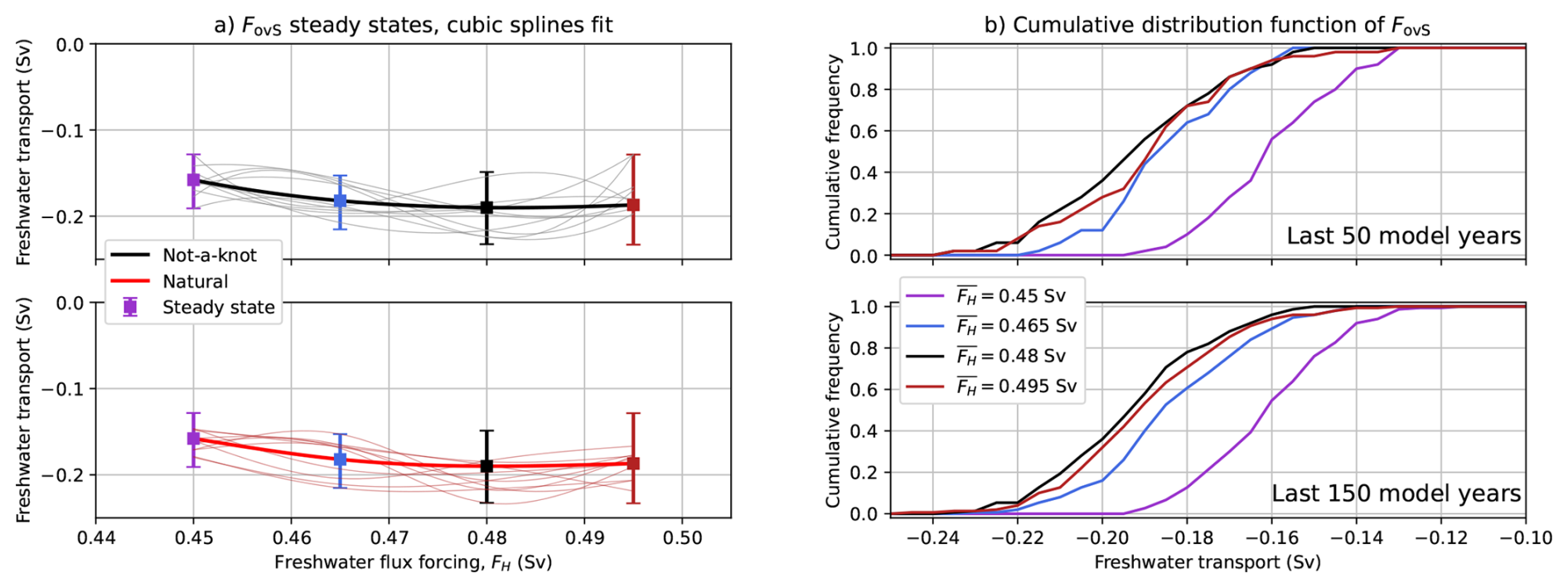
Figure 9 (a) Cubic splines fits (thin curves) using random F_ovS values from the four statistical equilibria. The mean over 100 000 random cubic splines are shown by the thick curves. We use the not-a-knot boundary condition (upper panel) and the natural boundary condition (lower panel). (b) The cumulative distribution function of the F_ovS for the four statistical equilibria, showing the last 50 model years (upper panel) and last 150 model years (lower panel).

The overlap in the statistical properties of the four statistical equilibria closest to the tipping point also complicates the shape (i.e., square-root) estimate between AMOC strength and F_H. These four equilibria are clearly insufficient and one needs more equilibria to obtain a better estimate of the shape. This is computationally expensive for the CESM, but can easily be done for the E-CCM and also under stochastic noise. Even if more equilibria were available for the CESM, there is a possibility that the structure of multiple equilibria is much more complicated (Lohmann et al., 2024). The latter may explain the relatively strong AMOC strength for $\stackrel{\mathrm{‾}}{F_H}=\mathrm{0.48}$ Sv, but this can not be verified from the results presented here. It is therefore more relevant to analyse the different AMOC feedback strengths over large F_H intervals, which clearly indicate a square root dependence between AMOC strength and F_H (Vanderborght et al., 2025) and this is also supported by the reduced model here.

Using the reduced model (with the c₁, c₂, g₁ and n₁ from the CESM), one can make a rough estimate of the critical freshwater flux forcing needed to collapse the present-day AMOC. For observed values, we used 17 Sv (Smeed et al., 2018) and −0.15 Sv (Arumí-Planas et al., 2024) for AMOC strength and F_ovS, respectively. We assume that all the Greenland Ice Sheet melt is added to the Atlantic Ocean surface, making the hosing 100 % effective, and we find $F_H^{\mathrm{c}}=\mathrm{0.19}$ Sv (Fig. 8). Although this critical freshwater flux forcing is substantially smaller than the CESM, it still boils down to 25 times the present-day melt rate of the Greenland Ice Sheet (Sasgen et al., 2020). Nevertheless, what is most relevant here is that the present-day AMOC is more sensitive (i.e., relatively large $\frac{\partial \mathrm{AMOC}}{\partial F_H}$) compared to CESM and typical CMIP6 models, as most climate models are positively biased in their F_ovS (van Westen and Dijkstra, 2024; van Westen et al., 2025b). In other words, the AMOC is overly stable when having positive F_ovS biases and underestimate the risk of AMOC tipping (Liu et al., 2017). As was argued in Vanderborght et al. (2025), the reduced model only holds under (quasi-)equilibrium conditions, making this analysis less useful under transient climate change (van Westen et al., 2025b).

5 Transient AMOC behavior under climate change

The existence of a saddle-node bifurcation in the E-CCM helps to understand how AMOC stability in CESM is influenced under climate change. Changes in the background climate conditions can be interpreted as a shift in the position of the saddle-node bifurcation. This can already be demonstrated in the Stommel model where the saddle-node bifurcation shifts to lower freshwater flux forcing values under a smaller atmospheric temperature gradient (Fig. A2).

We first analyse the CESM simulations under the Hist/RCP4.5 and Hist/RCP8.5 scenarios. The AMOC collapses in three out of the four CESM simulation under climate change (Fig. 10a, b). The simulation under the higher freshwater flux forcing of $\stackrel{\mathrm{‾}}{F_H}=\mathrm{0.45}$ Sv are closer to the tipping point (under PI conditions) and hence are more prone to undergo transitions, which is indeed the case. For $\stackrel{\mathrm{‾}}{F_H}=\mathrm{0.18}$ Sv, only the Hist/RCP8.5 scenario shows an AMOC collapse while in the Hist/RCP4.5 scenario the AMOC eventually recovers. In the latter scenario, the AMOC shows distinct centennial variability and this is associated with the typical overturning time scale (Winton and Sarachik, 1993).

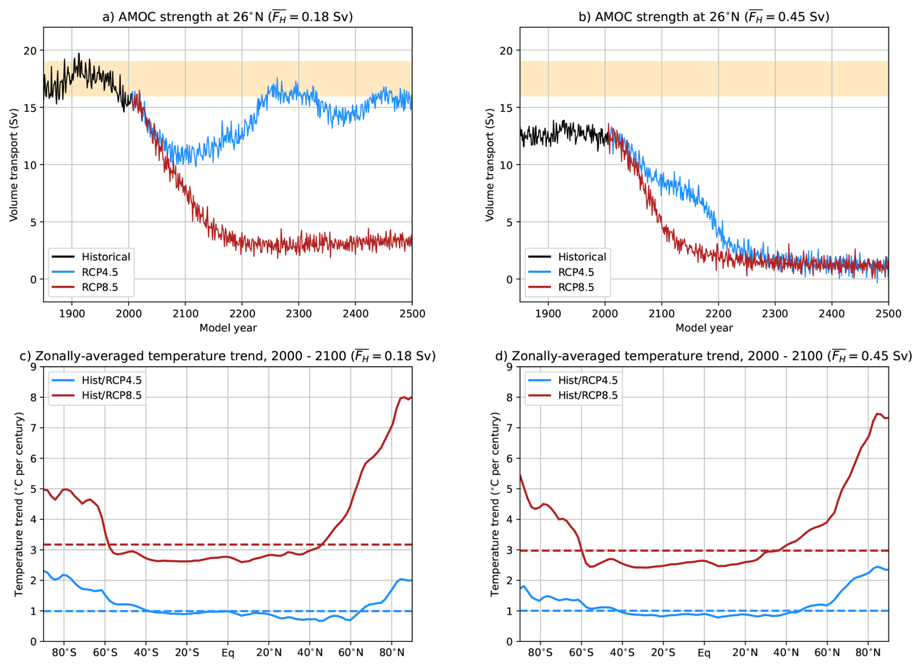
Figure 10 (a, b) The AMOC strength at 1000 m and 26° N under the different climate change scenarios, the yellow shading indicates observed ranges (Smeed et al., 2018). (c, d) The zonally-averaged (2 m) surface temperature trend (model year 2000–2100) under the different climate change scenarios. The globally-averaged temperature trend is indicated by the dashed lines.

The imposed transient climate change forcing induces above average surface temperature trends (compared to the global mean) at the higher latitudes (i.e., polar amplification, Fig. 10c, d). This temperature response reduces the meridional (equator-to-pole) temperature gradient and may influence the multi-stable AMOC regime, as is the case for the Stommel model (Fig. A2). We can test this in the E-CCM by reducing the atmospheric meridional temperature gradient by imposing a (positive) atmospheric temperature anomaly ($\mathrm{\Delta }{T}_{\mathrm{n}}^{\mathrm{a}}$) over box n (and also over atmospheric box s as they are coupled (van Westen et al., 2024b)). We keep the atmospheric temperatures the same for boxes t and ts to limit the degrees of freedom.

The steady states (with ξ=0) for the reference case ($\mathrm{\Delta }{T}_{\mathrm{n}}^{\mathrm{a}}=\mathrm{0}$ °C) and climate change case ($\mathrm{\Delta }{T}_{\mathrm{n}}^{\mathrm{a}}=\mathrm{5}$ °C) are shown in Fig. 11a. Both saddle-node bifurcations shift to lower E_A values and the hysteresis width decreases from 0.30 Sv (reference) to 0.22 Sv (climate change). This shift can be understood from the smaller meridional density difference between box n and box ts (Eq. 1) due to higher temperatures and this requires a smaller freshwater flux forcing to reach the critical AMOC strength corresponding to the tipping point. The reduced meridional temperature gradient also weakens the AMOC on strength by a few Sv when comparing the two cases. The shift of the upper saddle-node bifurcation to lower E_A values indicates that the AMOC on state loses stability under climate change.

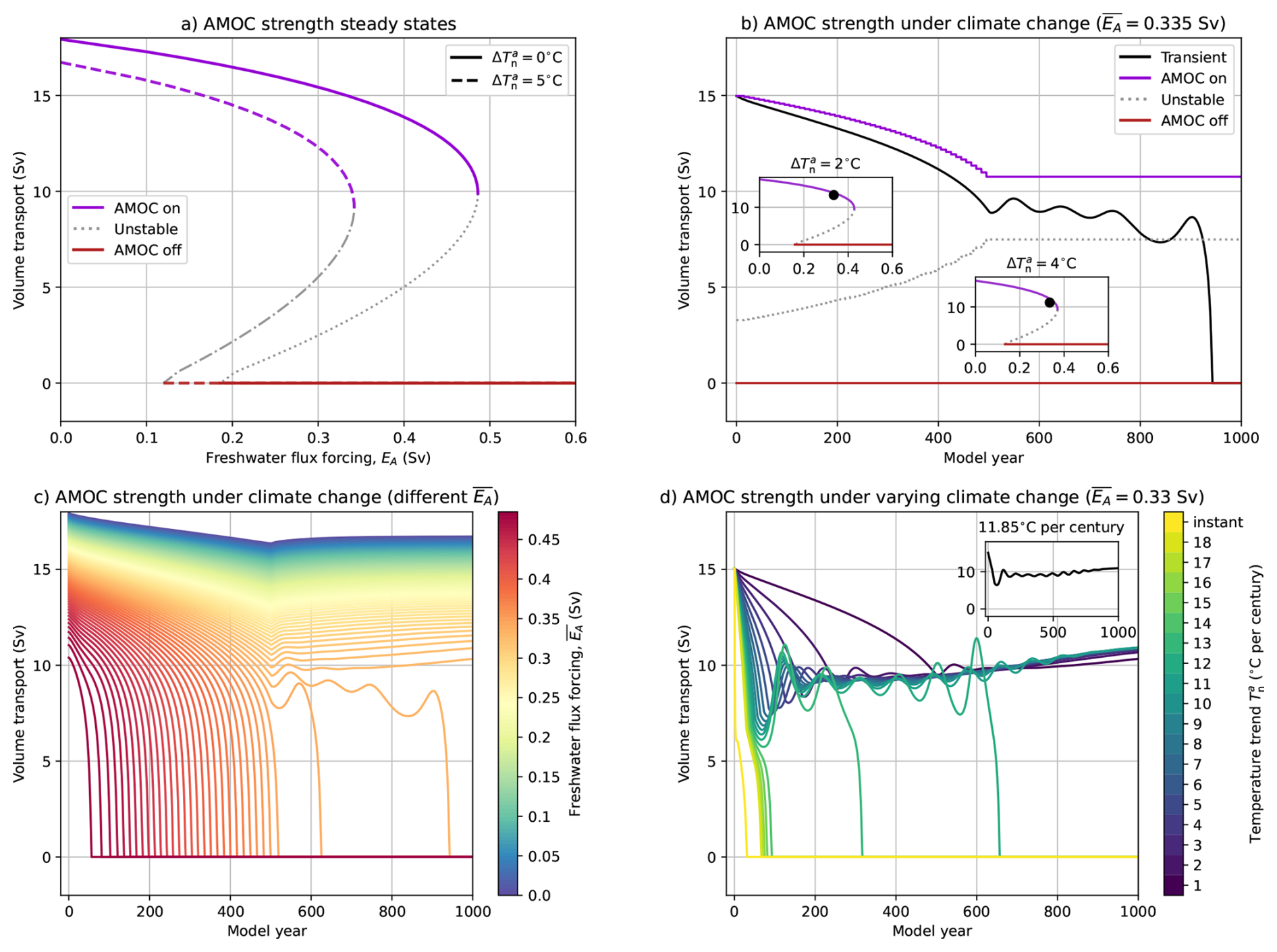
Figure 11 (a) The steady states for the AMOC strength for the standard set-up (solid curves) and under climate change (dashed curves). (b) The AMOC strength under transient climate change and $\stackrel{\mathrm{‾}}{E_{\mathrm{A}}}=\mathrm{0.335}$ Sv, where $\mathrm{\Delta }{T}_{\mathrm{n}}^{\mathrm{a}}$ linearly increases up to 5 °C up to model year 500 (trend of 1 °C per century) and then remains constant. The steady states at $\stackrel{\mathrm{‾}}{E_{\mathrm{A}}}=\mathrm{0.335}$ Sv for each climate change anomaly (with an accuracy of 0.1 °C) are also displayed. The insets show the steady states and the transient AMOC state (black dot) at $\mathrm{\Delta }{T}_{\mathrm{n}}^{\mathrm{a}}=\mathrm{2}$ °C (model year 200) and $\mathrm{\Delta }{T}_{\mathrm{n}}^{\mathrm{a}}=\mathrm{4}$ °C (model year 400). (c) Similar to panel b, but now for different values of $\stackrel{\mathrm{‾}}{E_{\mathrm{A}}}$ with $\mathrm{\Delta }\stackrel{\mathrm{‾}}{E_{\mathrm{A}}}=\mathrm{0.005}$ Sv. (d) The transient AMOC strength under climate change and $\stackrel{\mathrm{‾}}{E_{\mathrm{A}}}=\mathrm{0.33}$ Sv, but now for varying temperature trends in $\mathrm{\Delta }{T}_{\mathrm{n}}^{\mathrm{a}}$. The inset shows the transient AMOC strength for a temperature trend of 11.85 °C per century.

To study the transient climate change forcing in the E-CCM, we linearly increase $T_{\mathrm{n}}^{\mathrm{a}}$ by 1 °C per century up to model year 500 and then keep the temperature anomaly constant at $\mathrm{\Delta }{T}_{\mathrm{n}}^{\mathrm{a}}=\mathrm{5}$ °C. The AMOC strength (black curve in Fig. 11b) under climate change is shown for constant $\stackrel{\mathrm{‾}}{E_{\mathrm{A}}}=\mathrm{0.335}$ Sv, a similar set-up as in the CESM. For each temperature anomaly $\mathrm{\Delta }{T}_{\mathrm{n}}^{\mathrm{a}}$ we determined the steady states (with an accuracy of 0.1 °C) and the values for the AMOC on, unstable branch and AMOC off states for $\stackrel{\mathrm{‾}}{E_{\mathrm{A}}}=\mathrm{0.335}$ Sv are also shown in Fig. 11b. These steady states represent the “frozen” bifurcation diagrams for a given temperature anomaly (insets in Fig. 11b). The transient AMOC is clearly deviating from the AMOC on state. Up to model year 500, the AMOC gradually weakens and after a few oscillations eventually collapses in model year 900. These oscillations are related to a (sub-critical) Hopf bifurcation close to the saddle-node bifurcation. When lowering the $T_{\mathrm{n}}^{\mathrm{a}}$ trend to 0.726 °C per century and then keeping $\mathrm{\Delta }{T}_{\mathrm{n}}^{\mathrm{a}}=\mathrm{5}$ °C fixed, the AMOC strength also displays substantial oscillatory behaviour but does recover (not shown). This means that rate-induced effects are present and the AMOC collapses for $T_{\mathrm{n}}^{\mathrm{a}}$ trends larger than 0.726 °C per century for $\stackrel{\mathrm{‾}}{E_{\mathrm{A}}}=\mathrm{0.335}$ Sv.

When using a trend of 1 °C per century for $T_{\mathrm{n}}^{\mathrm{a}}$ (up to $\mathrm{\Delta }{T}_{\mathrm{n}}^{\mathrm{a}}=\mathrm{5}$ °C) and varying $\stackrel{\mathrm{‾}}{E_{\mathrm{A}}}$ (Fig. 11c), we always find an AMOC collapse for $\stackrel{\mathrm{‾}}{E_{\mathrm{A}}}>\mathrm{0.342}$ Sv as there are no stable AMOC on states at larger E_A values (Fig. 11a). The AMOC always recovers for $\stackrel{\mathrm{‾}}{E_{\mathrm{A}}}\le \mathrm{0.33}$ Sv, again demonstrating that rate-induced effects are present for $\stackrel{\mathrm{‾}}{E_{\mathrm{A}}}=\mathrm{0.335}$ Sv and $\stackrel{\mathrm{‾}}{E_{\mathrm{A}}}=\mathrm{0.34}$ Sv. Rate-induced effects are also present for $\stackrel{\mathrm{‾}}{E_{\mathrm{A}}}\le \mathrm{0.33}$ Sv, however, the AMOC is much more stable compared to the previous presented case of $\stackrel{\mathrm{‾}}{E_{\mathrm{A}}}=\mathrm{0.335}$ Sv. This is also demonstrated in Fig. 11d, where we vary the $T_{\mathrm{n}}^{\mathrm{a}}$ temperature trend and then keeping $\mathrm{\Delta }{T}_{\mathrm{n}}^{\mathrm{a}}=\mathrm{5}$ °C fixed for $\stackrel{\mathrm{‾}}{E_{\mathrm{A}}}=\mathrm{0.33}$ Sv. Oscillatory behaviour becomes more pronounced when increasing the $T_{\mathrm{n}}^{\mathrm{a}}$ temperature trend and the greatest AMOC weakening is found for relatively large temperature trends. For a temperature trend of 11.85 °C per century (inset in Fig. 11d), the AMOC strength (and other quantities) crosses the basin boundary between model years 43 and 87 and the AMOC displays oscillatory behavior. These oscillations decrease in amplitude after model year 800 and then the AMOC recovers. For larger temperature trends than 11.85 °C per century the AMOC eventually collapses, which is a factor of 16 larger than the critical temperature trend of 0.726 °C per century for $\stackrel{\mathrm{‾}}{E_{\mathrm{A}}}=\mathrm{0.335}$ Sv. This demonstrates that slightly lower E_A values can make the AMOC substantially more stable. It is possible to collapse the AMOC for $\stackrel{\mathrm{‾}}{E_{\mathrm{A}}}<\mathrm{0.33}$ Sv and this requires even larger climate change anomalies ($\mathrm{\Delta }{T}_{\mathrm{n}}^{\mathrm{a}}>\mathrm{5}$ °C).

6 Summary and Discussion

The Community Earth System Model (CESM) as used here (version 1.0.5) is an extremely high-dimensional dynamical system, representing the interaction of the ocean, atmosphere, land and sea-ice processes. In a pre-industrial configuration, the AMOC collapses under a quasi-equilibrium input of freshwater in the 20–50° N region, with surface freshwater compensation over the rest of the global domain (van Westen et al., 2024a).

In this paper, we have provided arguments for the case that, as in ocean-climate models lower in the model hierarchy (box models (Cessi, 1994) and fully-implicit ocean models (Dijkstra, 2007)), the AMOC collapse behavior in CESM is caused by the presence of a saddle-node bifurcation in the high-dimensional dynamical system. While one indeed would expect such a bifurcation in a deterministic dynamical system when varying a single parameter (where the saddle-node and the Hopf bifurcation are the only two generic codimension-1 bifurcations), this is far from trivial in the CESM. The ocean component of the CESM is much more complicated with several interacting positive and negative feedbacks (Vanderborght et al., 2025) and which is forced by a rapidly varying atmosphere. So attractors of the CESM are expected to have a quite complicated geometrical structure and transitions between those (such as between the AMOC on state and AMOC off state) could in principle be much more complicated than the traditional saddle-node bifurcation picture as suggested by conceptual models (Dijkstra, 2024).

For a saddle-node bifurcation, one would have to demonstrate a square root dependence of the AMOC strength on the freshwater forcing near the collapse point, which arises from the destabilising salt-advection feedback (Vanderborght et al., 2025). This is not feasible for the CESM due to its strong internal variability and hence our case is built using three more indirect arguments. The first argument is that in the CESM, there is a strict critical boundary of existence of the statistical steady “AMOC on” state. We showed this by subsequent near-equilibrium computations near the collapse point in the quasi-equilibrium simulation, similar to the approach in Hawkins et al. (2011). Such a strict boundary is characteristic of a saddle-node bifurcation as shown for the E-CCM. The full AMOC hysteresis experiment (van Westen and Dijkstra, 2023) shows that the AMOC recovers at a much lower freshwater flux forcing (F_H≈0.09 Sv) compared to the collapse point ($\mathrm{0.495}\le \stackrel{\mathrm{‾}}{F_H}<\mathrm{0.51}$ Sv), demonstrating non-linear behaviour that is also essential to saddle-node bifurcations. The second argument is based on the CESM results with a slower freshwater forcing rate. Here, we show that the AMOC collapse precisely follows the behaviour (Ritchie et al., 2021) one would expect near a saddle-node bifurcation, i.e., with a steeper transition (in F_H space) than for the standard forcing rate. Do note that this characteristics is also found for other bifurcation types (Berglund and Gentz, 2006). The third, and probably strongest, argument relies on the assumption that overturning freshwater transport predominately compensates any freshwater flux forcing, which holds approximately for the CESM (van Westen et al., 2024a). In this case, one can show that the AMOC strength has a square-root dependence with the freshwater forcing using a reduced model (cf. Sect. 4).

To these arguments, we can add the support from early warning indicators as found for the CESM (van Westen et al., 2024a). A characteristic property of saddle-node bifurcations is the loss of resilience (i.e., critical slowdown) near the tipping point, measured by the increase in variance and autocorrelation (van Westen et al., 2024b). Although these early warning indicators based on the AMOC strength were not giving any critical slowdown, optimal regions for early warning signal detection were found near 34° S (Smolders et al., 2025). The results presented here (cf. Fig. 3) show an increase in the F_ovS variance close to the tipping point. This increase in variability indicates that the AMOC loses resilience, making it more prone to transitions, characteristic of approaching a saddle-node bifurcation (van Westen et al., 2024b).

The implications of this result are substantial. First of all, it shows that, for the AMOC tipping problem, conceptual models that capture only the dominant feedbacks are useful (Dijkstra, 2024). For example, in the E-CCM only the salt-advection feedback and gyre feedback are captured which are also dominant in CESM and hence it is relatively easy to tune the behavior of the E-CCM to the CESM. Similarly, Wood et al. (2019) tuned a box model (only representing the salt-advection feedback) to the FAMOUS (Hawkins et al., 2011) where likely due to its low resolution the gyre feedback is relatively weak. Sensitivity studies in the conceptual model can then be used to design useful simulations in the complex model and also physical explanations can be sought in the reduced model. Second, if the multi-stable regime of the AMOC is bounded by saddle-node bifurcations, then the effect of model biases can be studied in terms of shifts of the saddle-node bifurcations. In fully-implicit ocean models, it was recently shown that a bias in Indian Ocean precipitation leads to a right shift (i.e., to higher Atlantic freshwater flux forcing strengths) of the bifurcation diagram (Dijkstra and van Westen, 2024; Boot and Dijkstra, 2025). Our reduced model (cf. Sect. 4.2) also shows that positive freshwater transport biases at 34° S make the AMOC more stable under hosing. If indeed a saddle-node bifurcation is present in all global climate models (GCMs), this would indicate that GCMs having such a bias would be too stable (van Westen and Dijkstra, 2024; van Westen et al., 2025b).

So far, the saddle-node bifurcation was discussed only in the case of an AMOC collapse when changing the freshwater flux forcing. However, under climate change mainly the heat flux forcing will change and not in a quasi-equilibrium way. Also in this case, we have shown that the existence of the saddle-node bifurcation is an important aspect to explain the transient behavior of the CESM. Climate change modifies the atmospheric meridional temperature gradient and shifts the saddle-node bifurcation to lower freshwater flux forcings, making the “AMOC on” state less resilient. This was shown in greater detail by the idealized results of the E-CCM, the collapse behavior can be viewed as crossing a moving saddle-node bifurcation in time (Ritchie et al., 2021). Rate-induced effects are also highly relevant under climate change (Hankel, 2025), with the strongest evidence for rate-induced tipping when comparing the RCP4.5 (AMOC recovery) and RCP8.5 (AMOC collapse) and $\stackrel{\mathrm{‾}}{F_H}=\mathrm{0.18}$ Sv. Although the AMOC collapses for both the RCP4.5 and RCP8.5 under $\stackrel{\mathrm{‾}}{F_H}=\mathrm{0.45}$ Sv, which suggests a moving saddle-node bifurcation under climate change, rate-induced effects cannot be dismissed and to test this we need to conduct more climate change forcing experiments, this is out of the scope of this paper. Note that the E-CCM is limited in representing other (non-linear) climate change feedbacks, such as enhanced evaporation (due to higher temperatures) which could partly stabilize the AMOC (van Westen et al., 2025b).

Finally, as the phase space of the CESM is so high-dimensional, why would a saddle-node bifurcation appear in such a model (as there are many instabilities)? This result can be possibly explained by looking at the Lorenz84-Stommel1961 model or the PlaSim sea-ice model (Tantet et al., 2018), which both display chaotic behavior, but also show a large-scale transition under variation of one parameter. Here, the chaotic behavior is only in the atmosphere component and the large-scale transition dynamics is governed only by the slow component, which is then noise-forced. While in the total phase space, this may be a crisis bifurcation, in the reduced phase space of the slow component, this would appear then as a saddle-node bifurcation. However, more work is needed to make this more precise.

Appendix A: The Analytical Solutions of the Stommel Box Model

The Stommel 2-box model (Stommel, 1961) consists of two well-mixed boxes (equal volume) and the boxes exchange water mass properties over time (Fig. A1). The circulation strength, ψ, is set by the density difference between the high-latitude (T₁, S₁) and equatorial box (T₂, S₂):

$$\begin{array}{}\text{(A1)}& \mathit{\psi }=k({\mathit{\rho }}_{\mathrm{1}}-{\mathit{\rho }}_{\mathrm{2}})\end{array}$$

where k is a hydraulic pumping constant. A linear equation of state ($\mathit{\rho }={\mathit{\rho }}_{\mathrm{0}}-\mathit{\alpha }(T-T_{\mathrm{0}})+\mathit{\beta }(S-S_{\mathrm{0}})$) yields:

$$\begin{array}{}\text{(A2)}& \mathit{\psi }=k(\mathit{\alpha }\mathrm{\Delta }T-\mathit{\beta }\mathrm{\Delta }S)\end{array}$$

where $\mathrm{\Delta }T=T_{\mathrm{2}}-T_{\mathrm{1}}$ and $\mathrm{\Delta }S=S_{\mathrm{2}}-S_{\mathrm{1}}$. The governing (dimensionless) differential equation for the Stommel model are then given by:

$$\begin{array}{}\text{(A3)}& {\displaystyle \frac{\mathrm{d}{T}_{\mathrm{1}}}{\mathrm{d}t}}=\left|\mathit{\psi }\right|\mathrm{\Delta }T+{\mathit{\lambda }}_T(T_{\mathrm{1}}^{\mathrm{a}}-T_{\mathrm{1}})\text{(A4)}& {\displaystyle \frac{\mathrm{d}{T}_{\mathrm{2}}}{\mathrm{d}t}}=-\left|\mathit{\psi }\right|\mathrm{\Delta }T+{\mathit{\lambda }}_T(T_{\mathrm{2}}^{\mathrm{a}}-T_{\mathrm{2}})\text{(A5)}& {\displaystyle \frac{\mathrm{d}{S}_{\mathrm{1}}}{\mathrm{d}t}}=\left|\mathit{\psi }\right|\mathrm{\Delta }S-\mathit{\eta }\text{(A6)}& {\displaystyle \frac{\mathrm{d}{S}_{\mathrm{2}}}{\mathrm{d}t}}=-\left|\mathit{\psi }\right|\mathrm{\Delta }S+\mathit{\eta }\end{array}$$

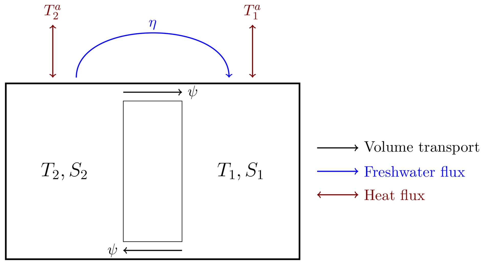
Figure A1 Schematic representation of the Stommel 2-box model in its northward overturning state with AMOC strength ψ. The blue and brown arrows are freshwater and heat fluxes, respectively. The hosing is directed from the equatorial box (with T₂, S₂) to the high-latitude box (with T₁, S₁).

In these relations λ_T is the thermal exchange coefficient with the overhead atmosphere, the atmospheric temperatures are fixed.

Under the assumption that the thermal exchange with the atmosphere is much faster than the thermal exchange between the boxes ($\mathit{\psi }\mathrm{\Delta }T\ll {\mathit{\lambda }}_T(T_i^{\mathrm{a}}-T_i)$, with $i=\mathrm{1},\mathrm{2}$), the steady state for the temperatures has $T_{\mathrm{1}}=T_{\mathrm{1}}^{\mathrm{a}}$ and $T_{\mathrm{2}}=T_{\mathrm{2}}^{\mathrm{a}}$. Using this steady state assumption, the time-evolution equation of the circulation strength (from Eqs. A2 and A3–A6) reduces to:

$$\begin{array}{}\text{(A7)}& \begin{array}{rl}{\displaystyle \frac{\mathrm{d}\mathit{\psi }}{\mathrm{d}t}}& =-k\mathit{\beta }{\displaystyle \frac{\mathrm{d}\mathrm{\Delta }S}{\mathrm{d}t}}=-k\mathit{\beta }\left({\displaystyle \frac{\mathrm{d}{S}_{\mathrm{2}}}{\mathrm{d}t}}-{\displaystyle \frac{\mathrm{d}{S}_{\mathrm{1}}}{\mathrm{d}t}}\right)\\ & =\mathrm{2}k\mathit{\beta }\left(\left|\mathit{\psi }\right|\mathrm{\Delta }S-\mathit{\eta }\right)\end{array}\end{array}$$

where the temperature contribution vanishes as the atmospheric temperatures are constant ($\frac{\mathrm{d}\mathrm{\Delta }T}{\mathrm{d}t}=\frac{\mathrm{d}\mathrm{\Delta }{T}^{\mathrm{a}}}{\mathrm{d}t}=\mathrm{0}$). The final step is to substitute $\mathrm{\Delta }S=\frac{k\mathit{\alpha }\mathrm{\Delta }{T}^{\mathrm{a}}-\mathit{\psi }}{k\mathit{\beta }}$ from Eq. (A2) to obtain:

$$\begin{array}{}\text{(A8)}& {\displaystyle \frac{\mathrm{d}\mathit{\psi }}{\mathrm{d}t}}=-\mathrm{2}\left|\mathit{\psi }\right|\mathit{\psi }+\mathrm{2}k\mathit{\alpha }\mathrm{\Delta }{T}^{\mathrm{a}}\left|\mathit{\psi }\right|-\mathrm{2}k\mathit{\beta }\mathit{\eta }\end{array}$$

The steady states ($\frac{\mathrm{d}\mathit{\psi }}{\mathrm{d}t}=\mathrm{0}$) with northward overturning (ψ>0) are given by:

$$\begin{array}{}\text{(A9)}& {\mathit{\psi }}_{\mathrm{1},\mathrm{2}}={\displaystyle \frac{k\mathit{\alpha }\mathrm{\Delta }{T}^{\mathrm{a}}}{\mathrm{2}}}\pm \sqrt{{\left({\displaystyle \frac{k\mathit{\alpha }\mathrm{\Delta }{T}^{\mathrm{a}}}{\mathrm{2}}}\right)}^{\mathrm{2}}-k\mathit{\beta }\mathit{\eta }}\end{array}$$

For the reversed circulation (ψ<0), these are:

$$\begin{array}{}\text{(A10)}& {\mathit{\psi }}_{\mathrm{3},\mathrm{4}}={\displaystyle \frac{k\mathit{\alpha }\mathrm{\Delta }{T}^{\mathrm{a}}}{\mathrm{2}}}\pm \sqrt{{\left({\displaystyle \frac{k\mathit{\alpha }\mathrm{\Delta }{T}^{\mathrm{a}}}{\mathrm{2}}}\right)}^{\mathrm{2}}+k\mathit{\beta }\mathit{\eta }}\end{array}$$

but note that ψ₃ has to be rejected since ψ₃≮0. The stable AMOC on state is given by ψ₁, the stable AMOC off state by ψ₄, and the unstable state by ψ₂. The (dimensionless) solutions for two different atmospheric temperature differences are shown in Fig. A2.

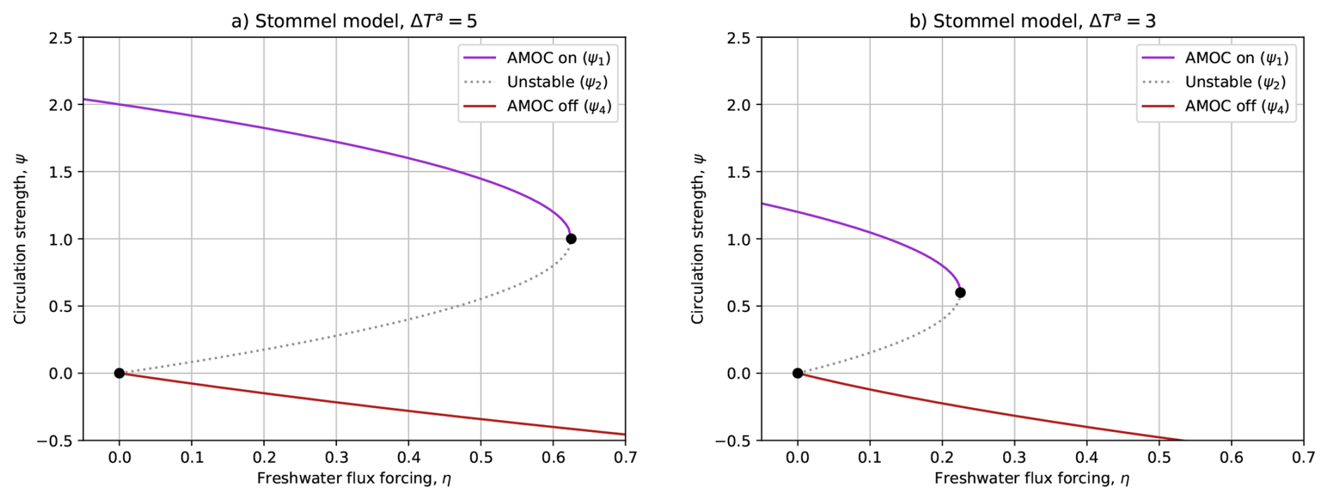
Figure A2 Bifurcation diagram for the Stommel 2-box model, where the black dots indicate saddle-node bifurcations. The atmospheric temperature differences are (a) ΔT^a=5 and (b) ΔT^a=3. For the other dimensionless coefficients, we used: $\mathit{\alpha }=\mathrm{2}\times {\mathrm{10}}^{-\mathrm{4}}$, $\mathit{\beta }=\mathrm{8}\times {\mathrm{10}}^{-\mathrm{4}}$ and $k=\mathrm{2}\times {\mathrm{10}}^{\mathrm{3}}$.

Appendix B: The Normal Form of the Saddle Node Bifurcation

For the Stommel model, the dynamics of the AMOC strength in the AMOC on state is given by:

$$\begin{array}{}\text{(B1)}& {\displaystyle \frac{\mathrm{d}\mathit{\psi }}{\mathrm{d}t}}=-\mathrm{2}{\mathit{\psi }}^{\mathrm{2}}+\mathrm{2}k\mathit{\alpha }\mathrm{\Delta }{T}^{\mathrm{a}}\mathit{\psi }-\mathrm{2}k\mathit{\beta }\mathit{\eta },\end{array}$$

which can be generalised for the saddle-node bifurcation to:

$$\begin{array}{}\text{(B2)}& {\displaystyle \frac{\mathrm{d}\mathit{\psi }}{\mathrm{d}t}}=A{\mathit{\psi }}^{\mathrm{2}}+B\mathit{\psi }+C-Dt.\end{array}$$

where A, B, C and D are constants, and the freshwater flux forcing is now varied linearly with time (i.e., η(t)=Dt). This generalised form also holds for the reduced model (Sect. 4.1).

Relation (B2) is rewritten as:

$$\begin{array}{}\text{(B3)}& {\displaystyle \frac{\mathrm{d}\mathit{\psi }}{\mathrm{d}t}}=A{\left(\mathit{\psi }+{\displaystyle \frac{B}{\mathrm{2}A}}\right)}^{\mathrm{2}}+\left(C-{\displaystyle \frac{B^{\mathrm{2}}}{\mathrm{4}A}}\right)-Dt.\end{array}$$

and we follow the procedure outlined in Faure Ragani and Dijkstra (2025), where time t is considered as a parameter and the saddle-node bifurcation can be found by setting the last two terms on the right hand side of (B3) to zero. Solving for t yields:

$$\begin{array}{}\text{(B4)}& t^{\mathrm{SN}}={\displaystyle \frac{C}{D}}-{\displaystyle \frac{B^{\mathrm{2}}}{\mathrm{4}AD}}.\end{array}$$

To obtain the normal form, we apply a rescaling of the variables:

$$\begin{array}{}\text{(B5)}& x=-A{t}^{\mathrm{SN}}\left(\mathit{\psi }+{\displaystyle \frac{B}{\mathrm{2}A}}\right)\mathrm{and}\mathit{\tau }={\displaystyle \frac{t}{t^{\mathrm{SN}}}}\end{array}$$

and the dynamics of the AMOC in the rescaled variables are:

$$\begin{array}{}\text{(B6)}& \begin{array}{rl}{\displaystyle \frac{\mathrm{d}x}{\mathrm{d}\mathit{\tau }}}& ={\displaystyle \frac{\mathrm{d}x}{\mathrm{d}t}}{\displaystyle \frac{\mathrm{d}t}{\mathrm{d}\mathit{\tau }}}=-A{t}^{\mathrm{SN}}{\displaystyle \frac{\mathrm{d}\mathit{\psi }}{\mathrm{d}t}}{t}^{\mathrm{SN}}\\ & =-A(t^{\mathrm{SN}}{)}^{\mathrm{2}}\left(A{\left(\mathit{\psi }+{\displaystyle \frac{B}{\mathrm{2}A}}\right)}^{\mathrm{2}}+\left(C-{\displaystyle \frac{B^{\mathrm{2}}}{\mathrm{4}A}}\right)-Dt\right).\end{array}\end{array}$$

Now using Eqs. (B4) and (B5) to find the normal form of:

$$\begin{array}{}\text{(B7)}& \begin{array}{rl}{\displaystyle \frac{\mathrm{d}x}{\mathrm{d}\mathit{\tau }}}& =-A(t^{\mathrm{SN}}{)}^{\mathrm{2}}\left(A{\displaystyle \frac{x^{\mathrm{2}}}{(-A{t}^{\mathrm{SN}}{)}^{\mathrm{2}}}}+D{t}^{\mathrm{SN}}-D{t}^{\mathrm{SN}}\mathit{\tau }\right)\\ & =r-x^{\mathrm{2}}\end{array}\end{array}$$

where $r=-AD(t^{\mathrm{SN}}{)}^{\mathrm{3}}\left(\mathrm{1}-\mathit{\tau }\right)$. Note that r>0 for τ<1 as A<0 and D>0.

The non-autonomous system (B7) can be solved analytically (Li et al., 2019) and it was shown that the collapse time $t^{*}=\mathrm{1}+\mathrm{2.333}{\mathit{\alpha }}^{-\mathrm{1}/\mathrm{3}}$, where $\mathit{\alpha }=-AD(t^{\mathrm{SN}}{)}^{\mathrm{3}}>\mathrm{0}$. If the forcing value at which the collapse occurs for a rate D is indicated by ${\mathit{\gamma }}_f=D{t}^{*}$, then for the collapse forcing (γ_s) at half rate $D/\mathrm{2}$, we find that α_s=4α_f and hence ${\mathit{\gamma }}_s=D(\mathrm{1}+\mathrm{2.333}{\mathit{\alpha }}_s^{-\mathrm{1}/\mathrm{3}})=D(\mathrm{1}+\mathrm{0.177}{\mathit{\alpha }}_f^{-\mathrm{1}/\mathrm{3}})<{\mathit{\gamma }}_f$. Hence, the transition occurs at lower forcing strength (and faster) when the rate is lower (see also Figs. 3b and  4 in Li et al. (2019)).