On a simplified solution of climate-carbon dynamics in idealized flat10MIP simulations

Idealized experiments with coupled climate-carbon Earth system models (ESMs) provide a basis for understanding the response of the carbon cycle to external forcing and for quantifying climate-carbon feedbacks. Here, we analyze globally-averaged results from idealized esm-flat10 experiments and show that most models exhibit a quasi-linear relationship between cumulative carbon uptake on land and in the ocean during a period of constant fossil fuel emissions of 10 Pg C yr⁻¹. We hypothesize that this relationship does not depend on emission pathways. Further, as a simplification, we quantify the relationship between cumulative ocean carbon uptake and changes in ocean heat content using a linear approximation. In this way, changes in oceanic heat content and atmospheric CO₂ concentration become interdependent variables, reducing the coupled temperature-CO₂ system to just one differential equation. The equation can be solved analytically or numerically for the atmospheric CO₂ concentration as a function of fossil fuel emissions. This approach leads to a simplified description of global carbon and climate dynamics, which could be used for applications beyond existing analytical frameworks.

1 Introduction

The relationship between climate change and carbon emissions has been extensively studied (Cox et al., 2000; Friedlingstein et al., 2006; Matthews and Zickfeld, 2012; Williams et al., 2016; Jones and Friedlingstein, 2020). The framework of idealized experiments of the Coupled Climate–Carbon Cycle Model Intercomparison Project (C4MIP) (Jones et al., 2016) allowed the climate-carbon feedback (Arora et al., 2020) to be quantified in the Coupled Model Intercomparison Project phase 6 (CMIP6) while experiments in the Zero Emissions Commitment Model Intercomparison Project (ZECMIP) helped to assessed the zero-emission climate commitment (Jones et al., 2019; MacDougall et al., 2020). Recently, “flat10” Model Intercomparison (flat10MIP) experiments (Sanderson et al., 2024) were conducted with a suite of ESMs to assess the carbon-climate dynamics relevant to mitigation (Sanderson et al., 2025). The core experiment in flat10MIP, esm-flat10, was designed to assess the response of temperature change and land/ocean carbon dynamics as a function of cumulative emissions. In this scenario, constant emissions of 10 Pg C yr⁻¹ continue for 100 years with the expectation of a near-linear increase in global temperature according to the concept of a constant Transient Climate Response to cumulative CO₂ Emissions (TCRE; Canadell et al., 2021). Here we evaluate the results of the flat10MIP experiments from participating models against a simple model of the energy and carbon budget of the coupled climate-carbon system.

These idealized climate-carbon experiments differ from historical CMIP6 experiments, where, in addition to the CO₂ forcing, historical forcings such as emissions of aerosols, non-CO₂ greenhouse gases and land-use changes were used for model evaluation against observed global and regional climate changes and atmospheric CO₂ concentrations.

For the carbon budget, historical simulations of ESMs were evaluated against observed atmospheric CO₂ concentration (Hajima et al., 2025) and results from stand-alone land and ocean carbon models which contributed to the Global Carbon Project (GCP; Friedlingstein et al., 2023). Idealized experiments cannot be directly evaluated against observations; however, they are very useful in understanding the role of different climate and carbon processes and the timescales of their dynamics.

The global energy balance of the climate system is a useful framework for analyzing climate models and observations (Forster et al., 2021; Gregory et al., 2009, 2024). Energy balance models assume that the Earth's annual energy budget was in equilibrium in the pre-industrial period, i.e., solar energy reaching the Earth was fully compensated by longwave radiation outgoing into space. The increase in greenhouse gases, especially CO₂, has disrupted this balance. The equation for the global energy balance can be formulated as follows:

$$\begin{array}{}\text{(1)}& N=F-\mathit{\lambda }T\end{array}$$

where N is the Earth's heat uptake, [W m⁻²], F is a forcing dependent on the anthropogenic greenhouse gases concentration in the atmosphere, [W m⁻²], λ is the climate feedback parameter, [W m⁻² K⁻¹], and T is the global temperature change relative to equilibrium [K]. Since the heat capacity of the land is negligible compared to the heat capacity of the ocean on annual time scales (Palmer and McNeall, 2014), the heat uptake could be interpreted solely as the heat uptake of the ocean (Gregory et al., 2024). The processes of oceanic heat uptake, mainly the warming of the mixed layer of the ocean and the transfer of heat to the deep ocean by convection and diffusion, are similar to the processes of inorganic oceanic carbon uptake (Seferian et al., 2024). The recently explored link between ocean warming and carbon uptake indicates a strong role of the Southern Ocean in the ocean carbon uptake (Williams et al., 2024; Bourgeois et al., 2022). In this study, we use the flat10 experiments to simplify the global dynamics and avoid going into such regional analyses. Winkler et al. (2024) showed that there is pathway-independent linear relationship between land and ocean carbon uptake in emission-driven simulations using the MPI Earth system model (MPI-ESM; Mauritsen et al., 2019). We generalize this empirical relationship and use it to simplify the energy budget model (Eq. 1) in such a way that it could be solved analytically or numerically, and then use the example of one model, MPI-ESM, to show how this approach could be applied to idealized experiments. We also use this simplified approach for the trajectory of the ramp-down scenario simulation of MPI-ESM and discuss our results. Afterwards, we apply this approach to some other flat10MIP ESMs and discuss analytical and numerical solutions for the airborne fraction of carbon emissions. Finally, we compare flat10MIP and C4MIP results and hypothesize about the dependence of idealized climate-carbon dynamics on CO₂ emission pathways.

2 Linking carbon cycle with ocean heat uptake

In differential equation form for the change in the ocean heat content (OHC) H, [J], Eq. (1) could be written as

$$\begin{array}{}\text{(2)}& {\displaystyle \frac{\mathrm{d}H}{\mathrm{d}t}}=F-\mathit{\lambda }T\end{array}$$

with initial conditions $H\left(\mathrm{0}\right)=T\left(\mathrm{0}\right)=\mathrm{0}$.

For the carbon cycle variables, let C_a, C_o, and C_l represent anthropogenic carbon content of the atmosphere, ocean, and land respectively, [Pg C], the initial values are zeros (pre-industrial equilibrium). Annual carbon emissions in the initial 100 years of flat10 experiments are prescribed at a constant rate of E=10 Pg C yr⁻¹ (Sanderson et al., 2024, 2025). For the flat10MIP analysis (Sanderson et al., 2025), most of the models show a linear relationship between cumulative land and ocean uptakes (Fig. 1):

$$\begin{array}{}\text{(3)}& C_{\mathrm{l}}\left(t\right)=(k-\mathrm{1})C_{\mathrm{o}}\left(t\right),\end{array}$$

where k is the ratio $(C_{\mathrm{l}}+C_{\mathrm{o}})/C_{\mathrm{o}}$ to be used in the equations hereafter. This linear relationship was also observed in a study using MPI-ESM and different idealized emission pathways (Winkler et al., 2024).

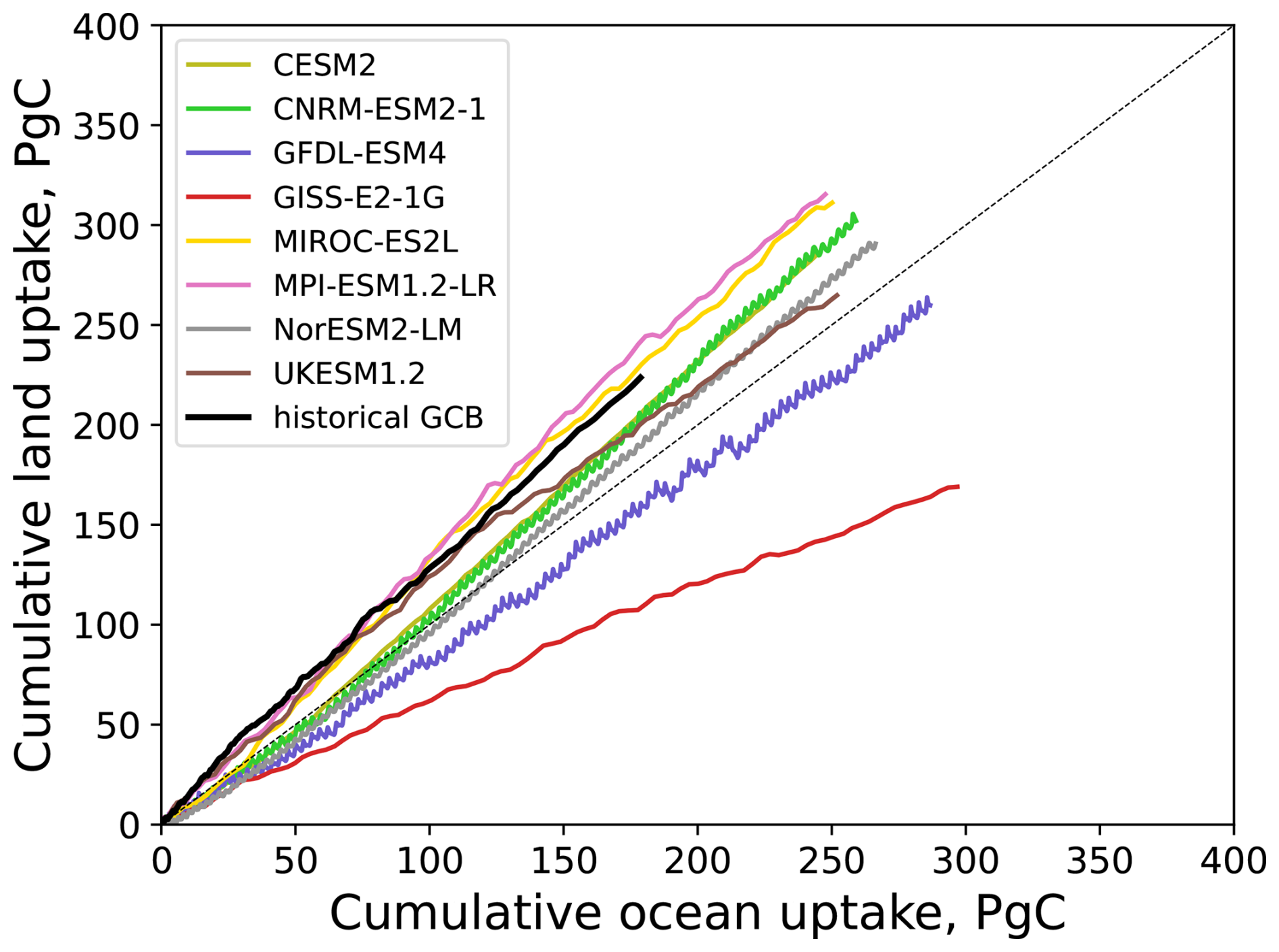
Figure 1 Cumulative land vs. ocean carbon uptakes in the flat10 experiments for the first 100 years. Historical land vs. ocean carbon sinks in the Global Carbon Budget (GCB) (Friedlingstein et al., 2023) for the period 1850–2022 are shown by continuous black line. The land sink in GCB is calculated from simulations in which CO₂ and climate evolved over the historical period, while the land cover stayed at its pre-industrial level (no land use change). The thin dash line is the 1:1 ratio.

Table 1 Parameters of flat10 ESMs. Left, $C_{\mathrm{l}}/C_{\mathrm{o}}=k-\mathrm{1}$, the ratio of cumulative land to ocean carbon uptakes by the year 100. For comparison with C4MIP experiments at the 2xCO₂ level (Arora et al., 2020): middle, ratio of β_l to β_o; right, a ratio of cumulative land to ocean carbon uptake.

* GISS model results are based on slightly older version of GISS-ESM.

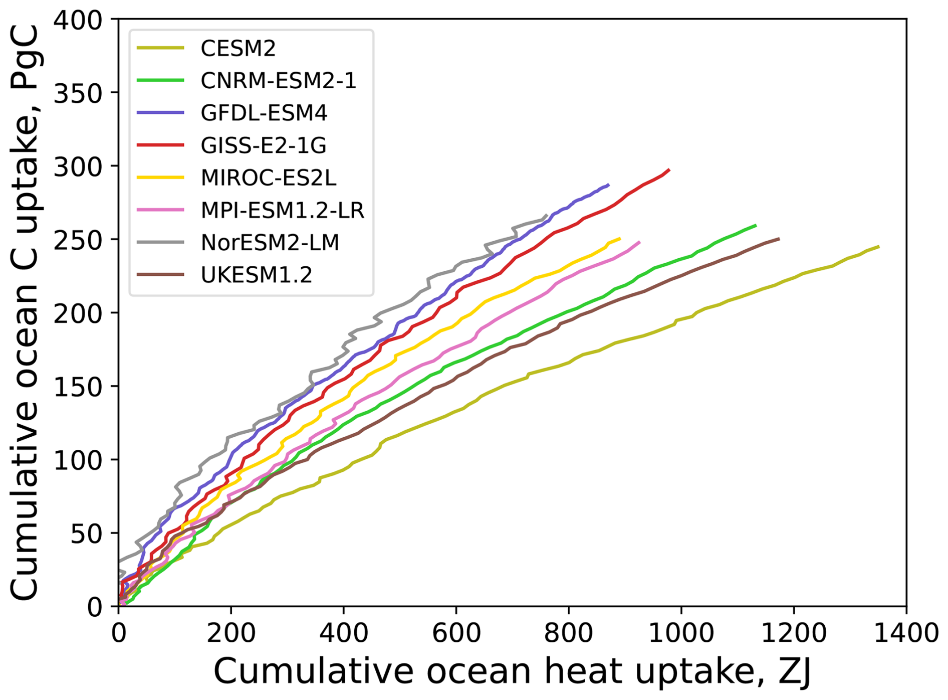
Figure 2 Changes in cumulative ocean carbon (Pg C) and heat uptakes (Zeta Joules) in the flat10 experiments.

The ratios of land to ocean carbon uptakes, $C_{\mathrm{l}}/C_{\mathrm{o}}$, in the flat10 experiments are similar to the ratios ${\mathit{\beta }}_{\mathrm{l}}/{\mathit{\beta }}_{\mathrm{o}}$ of the carbon–concentration feedback parameters as well as to the $C_{\mathrm{l}}/C_{\mathrm{o}}$ ratios at the 2xCO₂ level in the C4MIP experiments of CMIP6 (Table 1). This similarity is expected, as the carbon–concentration feedback parameters β_l and β_o reflect an increase of land and ocean carbon pools, respectively, in response to atmospheric CO₂ changes. However, the linearity of the $C_{\mathrm{l}}/C_{\mathrm{o}}$ ratio for the range of emissions from 0 to 1000 Pg C is unexpected. Although processes that govern land and ocean carbon uptakes are different, the link between them could be explained by increasing atmospheric CO₂ concentration which is a primary forcing for both land and ocean carbon uptakes. We can apply this empirical relationship to simplify the description of carbon cycle dynamics, in particular for MPI-ESM (Fig. 3, left). Additionally, for simplicity one can assume a linear relationship between ocean heat and carbon uptake, as the processes of dissolution and transport of CO₂ into the deep ocean are generally similar to the transport of heat (Figs. 2, 3, right):

$$\begin{array}{}\text{(4)}& C_{\mathrm{o}}\left(t\right)=\mathit{\eta }H\left(t\right),\end{array}$$

where the units of η are [Pg C J⁻¹]. Note that the ocean carbon sink saturates with rising CO₂ concentration and warming, therefore a non-linear logarithmic relationship between carbon and heat uptake might fit better (Fig. 2), but for simplicity we use the linear relationship (Eq. 4) thus allowing us to find an analytical solution of the coupled climate-carbon system. Note that the linear relationship is not valid for annual heat and carbon fluxes (Gillett, 2023) but it is appropriate for cumulative fluxes (Bronselaer and Zanna, 2020a).

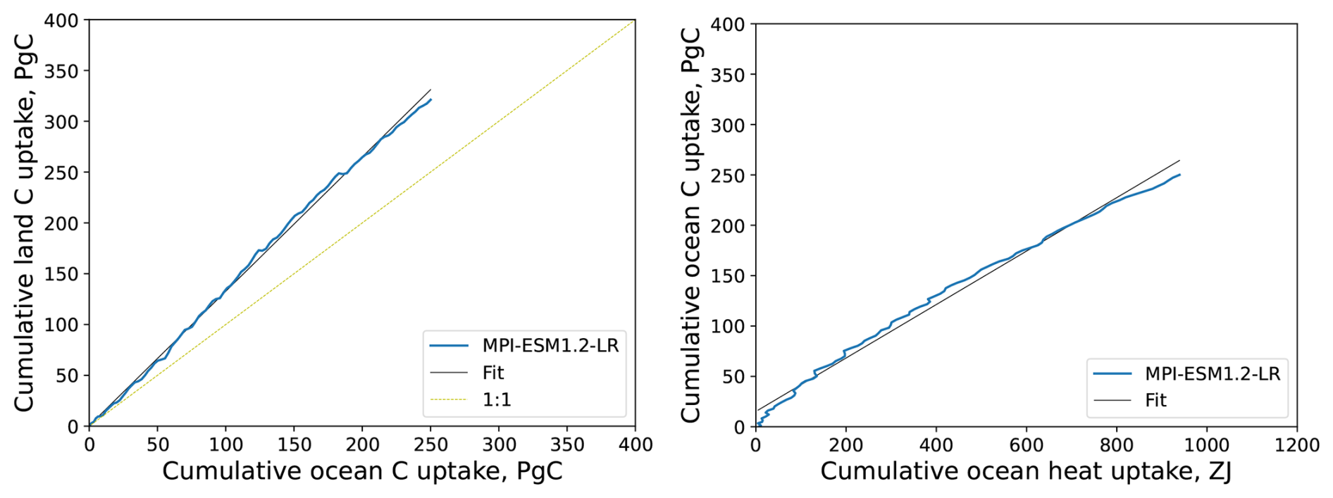
Figure 3 Results of the flat10 experiment with MPI-ESM1.2-LR (blue lines). Left: dynamics of cumulative land vs. ocean carbon uptakes. Right: changes in cumulative ocean carbon and heat uptakes. Black lines are for linear fits.

For the atmospheric carbon content, carbon conservation can be written as:

$$\begin{array}{}\text{(5)}& C_{\mathrm{a}}=Et-C_{\mathrm{l}}-C_{\mathrm{o}}=Et-k{C}_{\mathrm{o}}=Et-k\mathit{\eta }H\end{array}$$

where Et are the cumulative carbon emissions. The derivative of C_a is then

$$\begin{array}{}\text{(6)}& {\displaystyle \frac{\mathrm{d}{C}_{\mathrm{a}}}{\mathrm{d}t}}=E-k\mathit{\eta }{\displaystyle \frac{\mathrm{d}H}{\mathrm{d}t}}.\end{array}$$

From the Eq. (2), it follows

$$\begin{array}{}\text{(7)}& {\displaystyle \frac{\mathrm{d}{C}_{\mathrm{a}}}{\mathrm{d}t}}=E-k\mathit{\eta }(F-\mathit{\lambda }T).\end{array}$$

The Eq. (7), where left and right parts are functions of atmospheric CO₂ and time, reduces the coupled temperature-CO₂ system to just one differential equation. This is the novelty of our approach.

2.1 Analytical solution for the dynamical climate-carbon system with linear approximation of the forcing

We assume that the forcing F is linearly proportional to the CO₂ concentration, F=rC_a, where r is a constant [W m⁻² Pg C⁻¹], and that temperature is growing linearly with time as a consequence of constant TCRE (Transient Climate Response to cumulative CO₂ Emissions; Canadell et al., 2021). Accordingly, T=ζEt, where ζ=TCRE [K Pg C⁻¹], and we can write

$$\begin{array}{}\text{(8)}& {\displaystyle \frac{\mathrm{d}{C}_{\mathrm{a}}}{\mathrm{d}t}}=E-k\mathit{\eta }r{C}_{\mathrm{a}}+k\mathit{\eta }\mathit{\lambda }\mathit{\zeta }Et=E(\mathrm{1}+k\mathit{\eta }\mathit{\lambda }\mathit{\zeta }t)-k\mathit{\eta }r{C}_{\mathrm{a}}\end{array}$$

By renaming constants and writing x instead of C_a, this differential equation can be written in the form

$$\begin{array}{}\text{(9)}& {\displaystyle \frac{\mathrm{d}x}{\mathrm{d}t}}=k_{\mathrm{1}}+k_{\mathrm{2}}t+k_{\mathrm{3}}x\end{array}$$

where $k_i,i=\mathrm{1}$, 2, 3 are constants. By substituting the variable x to $u=k_{\mathrm{1}}+k_{\mathrm{2}}t+k_{\mathrm{3}}x$, Eq. (9) can be written as

$$\begin{array}{}\text{(10)}& {\displaystyle \frac{\mathrm{d}u}{\mathrm{d}t}}=k_{\mathrm{2}}+k_{\mathrm{3}}u\end{array}$$

and solved analytically. The solution for the coupled C_a and T system is

$$\begin{array}{}\text{(11)}& C_{\mathrm{a}}\left(t\right)=E\left({\displaystyle \frac{\mathit{\lambda }\mathit{\zeta }}{r}}t+{\displaystyle \frac{\left(r-\mathit{\lambda }\mathit{\zeta }\right)}{r^{\mathrm{2}}k\mathit{\eta }}}\left(\mathrm{1}-{\mathrm{e}}^{-k\mathit{\eta }rt}\right)\right)\end{array}$$

and

$$\begin{array}{}\text{(12)}& T\left(t\right)=\mathit{\zeta }Et.\end{array}$$

By renaming constants $\mathit{\phi }{}_{\mathrm{0}}=\frac{\mathit{\lambda }\mathit{\zeta }}{r}$, ${\mathit{\tau }}_{\mathrm{l}}=\frac{\left(r-\mathit{\lambda }\mathit{\zeta }\right)}{r^{\mathrm{2}}k\mathit{\eta }}$, ${\mathit{\tau }}_{\mathrm{e}}=\frac{\mathrm{1}}{k\mathit{\eta }r}$, Eq. (11) can be written as

$$\begin{array}{}\text{(13)}& C_{\mathrm{a}}\left(t\right)=Et\left({\mathit{\phi }}_{\mathrm{0}}+{\displaystyle \frac{{\mathit{\tau }}_{\mathrm{l}}}{t}}(\mathrm{1}-{\mathrm{e}}^{-t/{\mathit{\tau }}_{\mathrm{e}}})\right)=Et\mathit{\phi }\left(t\right),\end{array}$$

where $\mathit{\phi }\left(t\right)=\mathit{\phi }{}_{\mathrm{0}}+\frac{{\mathit{\tau }}_{\mathrm{l}}}{t}(\mathrm{1}-{\mathrm{e}}^{-t/{\mathit{\tau }}_{\mathrm{e}}})$ is the airborne fraction of cumulative CO₂ emissions, φ₀ is the asymptotic airborne fraction, τ_l and τ_e are, respectively, linear and exponential time scales of the exponential component of the airborne fraction, [years]. Values of parameters φ₀, τ_l and τ_e for ESMs are given in the Table 2. The airborne fraction at t=0 is about one because emissions are added to the atmosphere and it takes time for land and ocean carbon cycles to respond to the rising atmospheric CO₂ concentration.

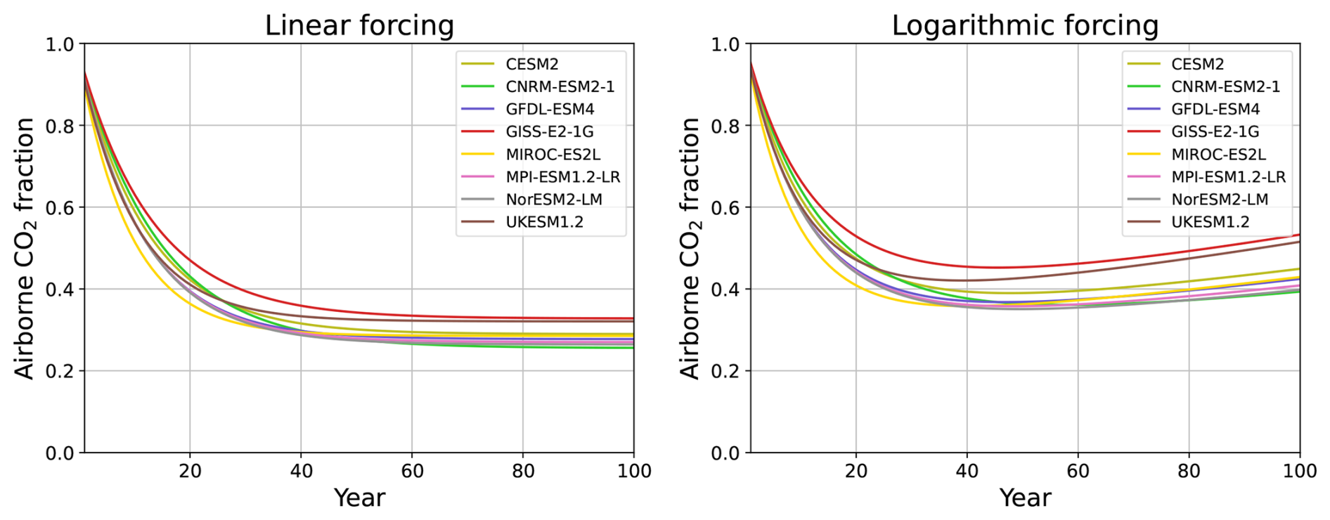
Figure 4 Instantaneous CO₂ airborne fraction in the analytical (left) and numerical (right) solutions for flat10 ESMs.

According to Eq. (13), the cumulative airborne CO₂ fraction, φ(t) includes two terms. The first term φ₀ is a constant, and the second term $\frac{{\mathit{\tau }}_{\mathrm{l}}}{t}(\mathrm{1}-{\mathrm{e}}^{-t/{\mathit{\tau }}_{\mathrm{e}}})$ is time-dependent. Because the latter is proportional to $\frac{\mathrm{1}}{t}$, it decreases with time, therefore, the cumulative airborne fraction φ(t) also decreases with time. The instantaneous airborne fraction φ_i can be written as

$$\begin{array}{}\text{(14)}& \mathit{\phi }{}_i\left(t\right)={\displaystyle \frac{\mathrm{d}{C}_{\mathrm{a}}}{\mathrm{d}t}}{\displaystyle \frac{\mathrm{1}}{E}}=\mathit{\phi }{}_{\mathrm{0}}+{\displaystyle \frac{{\mathit{\tau }}_{\mathrm{l}}}{{\mathit{\tau }}_{\mathrm{e}}}}{\mathrm{e}}^{-t/{\mathit{\tau }}_{\mathrm{e}}}\end{array}$$

Because the exponential term ${\mathrm{e}}^{-t/{\mathit{\tau }}_{\mathrm{e}}}$ is decreasing with time, the instantaneous airborne fraction also decreases with time approaching φ₀ (Fig. 4, left). The land and ocean carbon storages can be written as

$$\begin{array}{}\text{(15)}& C_{\mathrm{l}}\left(t\right)={\displaystyle \frac{k-\mathrm{1}}{k}}\left(Et-C_{\mathrm{a}}\right)\end{array}$$

and

$$\begin{array}{}\text{(16)}& C_{\mathrm{o}}\left(t\right)={\displaystyle \frac{\mathrm{1}}{k}}\left(Et-C_{\mathrm{a}}\right),\end{array}$$

and the derivative of atmospheric CO₂ with respect to temperature:

$$\begin{array}{}\text{(17)}& {\displaystyle \frac{\mathrm{d}{C}_{\mathrm{a}}}{\mathrm{d}T}}={\displaystyle \frac{\mathrm{d}{C}_{\mathrm{a}}}{\mathrm{d}t}}{\displaystyle \frac{\mathrm{d}t}{\mathrm{d}T}}={\displaystyle \frac{\mathit{\lambda }}{r}}+{\displaystyle \frac{\left(r-\mathit{\lambda }\mathit{\zeta }\right)}{r\mathit{\lambda }}}{\mathrm{e}}^{-k\mathit{\eta }rt}.\end{array}$$

These results can be used to understand the dynamics of carbon feedback parameters.

2.2 Numerical solution with forcing as logarithmic function of CO₂

The assumption that the forcing F is linearly proportional to the CO₂ concentration, F=rC_a, is only valid for small changes in CO₂. More correctly, a logarithmic dependence $F=r\ln (\mathrm{1}+\frac{C_{\mathrm{a}}}{C_{\mathrm{a}}^{\mathrm{0}}})$, where $C_{\mathrm{a}}^{\mathrm{0}}$ is pre-industrial atmospheric CO₂ storage, leads to an equation in the form:

$$\begin{array}{}\text{(18)}& {\displaystyle \frac{\mathrm{d}x}{\mathrm{d}t}}=k_{\mathrm{1}}+k_{\mathrm{2}}t+k_{\mathrm{3}}\ln (\mathrm{1}+x)\end{array}$$

which does not have an analytical solution.

The equation for atmospheric CO₂ concentration:

$$\begin{array}{}\text{(19)}& {\displaystyle \frac{\mathrm{d}{C}_{\mathrm{a}}}{\mathrm{d}t}}=E-k\mathit{\eta }r\ln \left(\mathrm{1}+{\displaystyle \frac{C_{\mathrm{a}}}{C_{\mathrm{a}}^{\mathrm{0}}}}\right)+k\mathit{\eta }\mathit{\lambda }\mathit{\zeta }Et\end{array}$$

can be solved using a numerical approach. Equations (15) and (4) provide solutions for carbon and heat variables, respectively. Accounting for the logarithmic dependence of the forcing on CO₂ results in much better agreement with the MPI-ESM simulation (see Fig. 5, left). The cumulative airborne CO₂ fraction is decreasing until about year 40 for MPI-ESM and then starts to increase slowly (Fig. 4, right). This is different from the airborne CO₂ fraction of the analytical solution that continues to decline (Fig. 4, left). Results of the analytical and numerical solutions for several other flat10 ESMs are presented on the Fig. 6. The actual airborne fraction is the same as on the Fig. 4 (right) because the atmospheric CO₂ dynamics are captured well in the numerical solutions with logarithmic CO₂ forcing as shown on the Fig. 6.

An analysis of the airborne CO₂ fraction in the analytical and numerical solutions revealed an important explanation for the linearity of the TCRE. If the radiative forcing were linearly dependent on the atmospheric CO₂ concentration, the airborne fraction would stabilize at a certain level. TCRE is constant in this case (Eq. 12). The realistic, logarithmic dependence of the radiative forcing on the CO₂ concentration leads to the airborne fraction increasing after 30–40 years of emissions. With increasing atmospheric CO₂ level, the weakening CO₂ radiative forcing is therefore compensated by an increasing airborne CO₂ fraction, which leads to an almost constant temperature increase per unit of emissions or constant TCRE.

Figure 5 Atmospheric CO₂ concentration in the flat10 (left) and flat10cdr (right) experiments with MPI-ESM (black). Blue and orange lines are for analytical and numerical solutions, respectively.

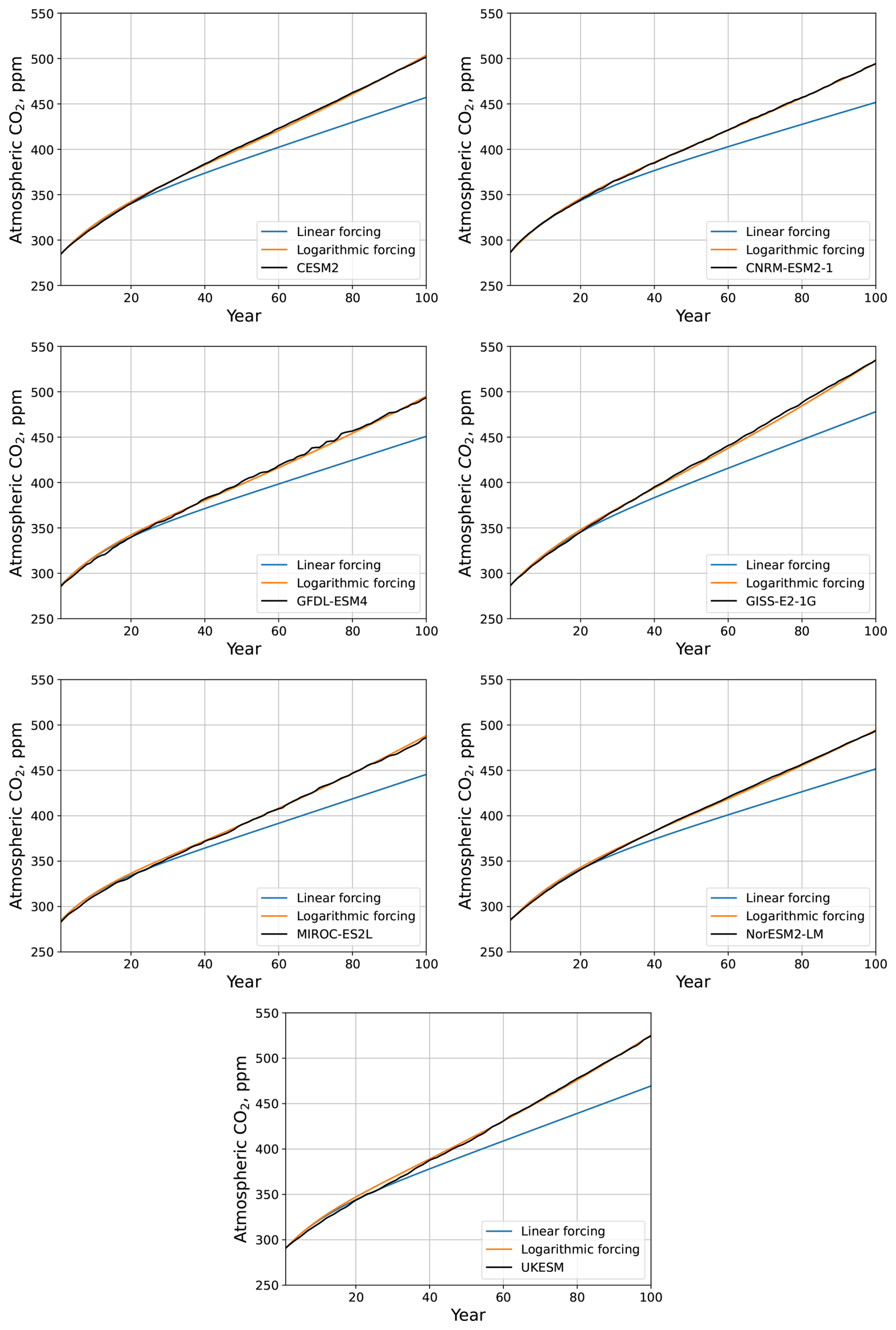
Figure 6 Atmospheric CO₂ concentration in the flat10 experiment with ESMs (black) and model results (blue: analytical, orange: numerical solution).

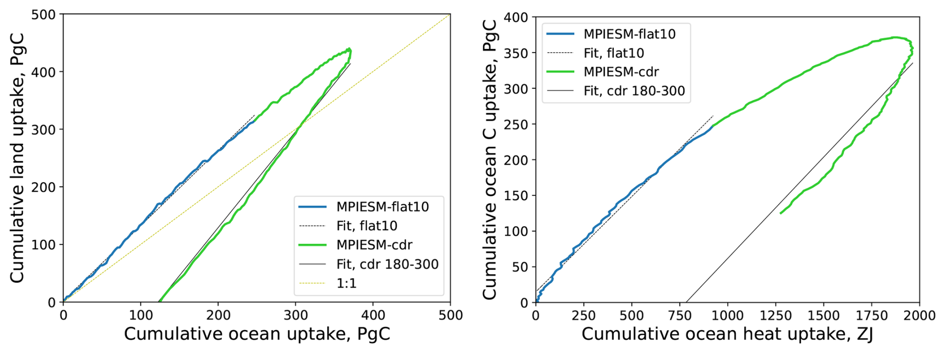
Figure 7 Cumulative land to ocean carbon uptakes (left) and ocean carbon to heat uptakes (right) in the flat10 and flat10cdr experiments with MPI-ESM1.2-LR. Gray lines are linear fits for the corresponding simulations.

Table 2 Parameters of airborne fraction of atmospheric CO₂ for flat10 ESMs. Left, φ₀, an asymptotical airborne fraction; middle, τ_l, linear airborne timescale; right, τ_e, exponential airborne timescale.

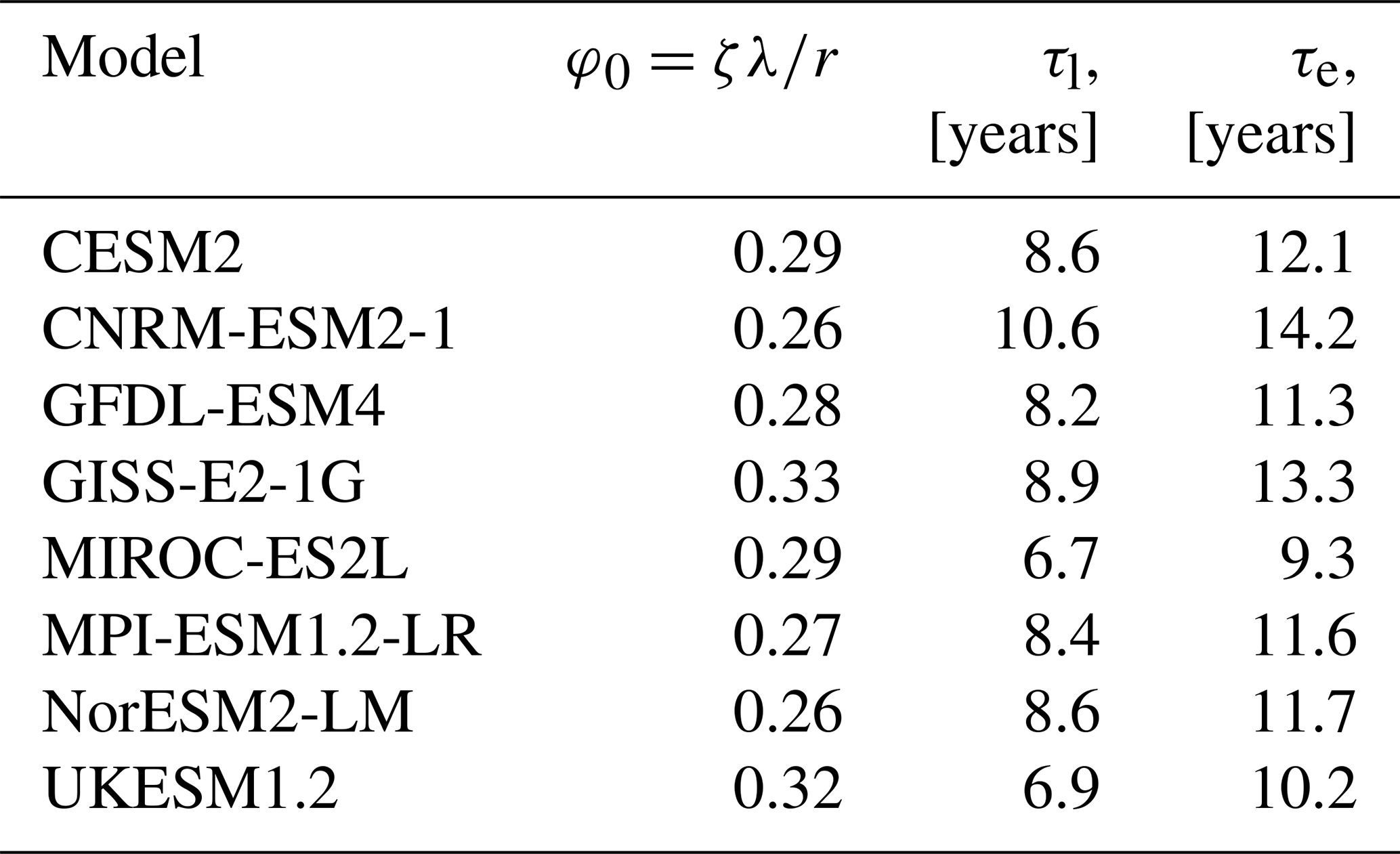
Table 3 Parameters based on flat10 experiments: $C_{\mathrm{l}}/C_{\mathrm{o}}$, the ratio of cumulative land to ocean carbon uptake (year 100); $C_{\mathrm{o}}/\text{OHC}$, the ratio of cumulative ocean carbon to heat uptake, Pg C ZJ⁻¹ (year 100); TCRE, K Eg C⁻¹ (year 100); and λ from 4xCO₂ experiments (Zelinka et al., 2020). Numbers in parentheses are adjusted parameters for analytical and numerical solutions.

2.3 Ramp-down flat10cdr experiments

Beyond 100 years of flat10 simulations (ramp-up), the flat10MIP experiments also included flat10cdr simulations for a further 200 years aiming to assess time scales and hysteresis in climate and carbon variables. The flat10cdr scenario included a linear decrease in emissions from +10 to −10 Pg C per year over 100 years and constant −10 Pg C emissions (removed from the atmosphere) over the next 100 years (ramp-down trajectory). The results for carbon and heat uptake for the MPI-ESM are shown in the Fig. 7. The ramp-down dynamics are quasi-linear for both the carbon variables and the ocean heat content, although the statistical significance of fits is lower than for the ramp-up curve. With the simplified approach (Eqs. 9–18), modified parameters (k=2.4 and η=0.22 Pg C ZJ⁻¹) and initial conditions matching the flat10cdr simulation at the year 200 (T=1.3 K, CO₂ concentration of 385 ppm), we are able to simulate the atmospheric CO₂ trajectory for the last 100 years of the flat10cdr experiment quite well (Fig. 5, right). This indicates that the dynamics with constant negative emissions could be simplified in a similar way to the path with positive emissions. This approach captures well the ramp-down trajectory for constant emissions but not the earlier part of trajectory with emissions changing from 10 to −10 Pg C yr⁻¹.

3 Discussion

The analysis of the idealized flat10 experiments helps to evaluate a simplified formulation of the coupled climate-carbon dynamics. In particular, the linear relationship between the cumulative carbon uptake of land and ocean is a remarkable feature of the dynamics of the global carbon cycle, independent of the emission pathway (Winkler et al., 2024). Except for that recent study, it has not been been discussed in previous publications examining idealized CO₂ experiments. Interestingly, $C_{\mathrm{l}}/C_{\mathrm{o}}$ dynamics are also linear in experiments with a 1 % annual increase in CO₂ concentration (Arora et al., 2020) up to a CO₂ concentration of about 2xCO₂ (Fig. A1, left). The $C_{\mathrm{l}}/C_{\mathrm{o}}$ ratio in emission-driven flat10 experiments and concentration-driven C4MIP experiments is very similar (Table 1). This indicates that the $C_{\mathrm{l}}/C_{\mathrm{o}}$ ratio only weakly dependent on idealized emission scenarios and that $C_{\mathrm{l}}/C_{\mathrm{o}}$ does not differ significantly between concentration- and emission-driven simulations. The study by Winkler et al. (2024) confirmed this for the MPI-ESM model (see Fig. A2). Since we did not perform a full set of simulations with different idealized scenarios, we cannot prove this for all models, but formulate these results as a set of hypotheses:

• Hypothesis I: $C_{\mathrm{l}}/C_{\mathrm{o}}$ does not differ between idealized emission scenarios,

• Hypothesis II: $C_{\mathrm{l}}/C_{\mathrm{o}}$ does not differ significantly between concentration- and emission-driven idealized simulations.

There are clear limits to the validity of these hypotheses. Firstly, they are based on simulations spanning only a 100 year period (for some models, longer simulations are provided). Secondly, the linear relationship is known to hold for most models up to emissions of at least 1000 Pg C or a CO₂ concentration of about 560 ppmv. At higher CO₂ concentrations, carbon uptake on land in some models increases more slowly or even decline compared to ocean uptake (Sanderson et al., 2025), $C_{\mathrm{l}}/C_{\mathrm{o}}$ decreases or reverses, and the relationship becomes non-linear (Fig. A1, right) as also reported by Winkler et al. (2024) for different pathways. This non-linear behavior usually emerges at high atmospheric CO₂ (and temperature) level, potentially due to saturation in CO₂ fertilization- or nutrient limitation-associated vegetation growth (Arora et al., 2020; Tjiputra et al., 2025; Kou-Giesbrecht et al., 2025).

An exception is the ACCESS model, one of the flat10 and C4MIP models, which shows no linear relationship after about 30 years of experimentation (Fig. A3). In all ACCESS-ESM1.5 CMIP6 runs and the flat10 simulations, phosphorus limitation was accounted for and it has limited the land carbon uptake. However, this is not the main reason for the non-linear behaviour. The saturation in cumulative land carbon uptake in the ACCESS model is partly due to a relative increase in heterotrophic respiration (R_h) in response to temperature (Ziehn et al., 2021), which has a delayed impact due to large carbon pool turnover times. Also, temperature might be limiting carbon uptake in the tropics because optimal temperature for photosynthesis is exceeded and productivity therefore declines, while R_h is increasing. These non-linear dynamics deviate from the historical trajectory of the global carbon budget (Friedlingstein et al., 2023) indicated by black lines on the Fig. A3. Therefore, we excluded this model from our analysis of climate-carbon dynamics. It is noteworthy that the trajectories of the ACCESS model are very similar for concentration- and emission-driven experiments (Fig. A3). Despite the ACCESS model behaving differently than the other models, this fact supports hypotheses I and II.

The quasi-linear $C_{\mathrm{l}}/C_{\mathrm{o}}$ relationship allows a simplified analysis of the energy budget of the system. The relationship between ocean carbon and ocean heat uptake is less linear, but a linear assumption helps to simplify the coupled energy and carbon dynamics. For MPI-ESM, the simplified approach with parameters from the flat10 and 4xCO₂ experiments (used for determining the climate feedback) leads to a very good fit of the atmospheric CO₂ concentration (Fig. 5). For the other models, a good fit to the atmospheric CO₂ concentrations (Fig. 6) requires an adjustment of the climate feedback parameters, mostly towards higher values (Table 3). This possible mismatch could be explained by the non-linearity of the relationship between carbon and heat in the ocean and/or by the higher values of the climate feedbacks for the first years of the 4xCO₂ experiment (Zelinka et al., 2020).

The airborne CO₂ fraction in the analytical solution decreases over time (and with increasing emissions) until it stabilizes at a certain level (Fig. 4, left). This behavior sounds counterintuitive, as feedback analysis of the climate-CO₂ relationship (Friedlingstein et al., 2006; Arora et al., 2020) suggests that the airborne fraction should increase and not decrease with increased emissions and temperatures. Under the analytical assumptions, however, this makes sense: with a linearly increasing CO₂ forcing, heat uptake increases, leading to increased carbon uptake in the ocean and on land. However, since the radiative forcing depends logarithmically on CO₂, the proportion of CO₂ left in the air initially decreases in the simulations, and then increases after 30–50 years in all ESMs (Fig. 4, right). It is interesting to note that this non-linearity in the dependence of radiative forcing on CO₂ leads to lower carbon uptake in the ocean and on land than the linear dependence of radiative forcing.

The main mechanisms of carbon uptake on land are CO₂ fertilization of plant productivity (which increases logarithmically with increasing CO₂ concentration) and heterotrophic or soil respiration (which increases exponentially with increasing soil temperature). The net effect is an increase in carbon uptake with elevated CO₂, with a tendency for land carbon uptake to slow as warming progresses (Canadell et al., 2021). There are also other less significant processes such as disturbances and shifts in vegetation distribution that affect carbon changes on land. For example, Winkler et al. (2024) demonstrated that vegetation dynamics lead to an additional increase in forest carbon storage.

In the ocean, CO₂ uptake is mainly determined by the CO₂ pressure difference between the atmosphere and the surface water and by the diffusion/removal of dissolved inorganic carbon (DIC) into the permanent thermocline. With increased temperature and elevated DIC concentration, the CO₂ solubility in sea water decreases and ocean uptake slows down. Changes in marine biology also affect carbon uptake, but to a lesser extent (Williams et al., 2020; Seferian et al., 2024; Tjiputra et al., 2025). An implication of the linear relationship between cumulative land and ocean uptakes (Fig. 1) is that mechanisms either don't change much, or slow at the same rate for ocean and land. This is consistent with the notion that global rates of heat and carbon uptake by the ocean are primarily set by the background, or unperturbed, ocean circulation (Armour et al., 2016; Bronselaer and Zanna, 2020b). This might help explain why the relation between cumulative heat and carbon uptake is scenario-independent in MPI-ESM (Fig. A2), as future rates of heat and carbon uptake are largely unaffected by changes in the ocean circulation. Whether or not ocean dynamical adjustments can break this linearity over longer timescales merits further analysis but is beyond the scope of this paper.

4 Conclusions

The relationship between cumulative carbon uptake on land and in the ocean, $C_{\mathrm{l}}/C_{\mathrm{o}}$, is model-specific and nearly linear in flat10 simulations until it reaches twice the pre-industrial CO₂ concentration. Comparison of emission-driven flat10MIP and concentration-driven C4MIP simulations shows that the $C_{\mathrm{l}}/C_{\mathrm{o}}$ relationship is the same regardless of whether atmospheric CO₂ is prescribed or interactive. Experiments with different Earth system models suggest that this relationship is also independent of the emission pathways. Therefore, we have formulated the hypothesis that the relationship $C_{\mathrm{l}}/C_{\mathrm{o}}$ is independent of the carbon cycle models used in each ESM. The validity of this hypothesis is subject to certain limitations, in particular the linearity does not work well for CO₂ concentrations above twice the pre-industrial CO₂ level. A further limitation arises from the hundred-year duration of the flat10 simulations, as adjustments in the deep ocean on a time scale of 500–1000 years will significantly alter the carbon cycle and the temperature response.

We also found a relationship between ocean heat and carbon uptake in idealized simulations that allows for a simplification of the coupled climate-carbon dynamics. This approach links the atmospheric CO₂ concentration to the ocean heat uptake and allows a reduction of the dynamical system to fewer variables. The simplified approach is valid for both ramp-up and ramp-down experiments.

While our approach exploits a linear response of the climate-carbon cycle system to the CO₂ forcing, the nonlinearity of the climate system is confirmed by past climate records (Brovkin et al., 2021). Therefore, the linearity assumption applies within a certain range of climate change, which is still uncertain but under active investigation (Winkelmann et al., 2025).

Appendix A

For comparison with the flat10 experiments, the results of the C4MIP simulations are shown in Figs. A1 and A3. Notations and parameter units are listed in the Table A1.

Figure A1 Cumulative land vs. cumulative ocean carbon uptake in the C4MIP experiments up to 2xCO₂ (left) and up to 4xCO₂ levels (right), data from Arora et al. (2020).

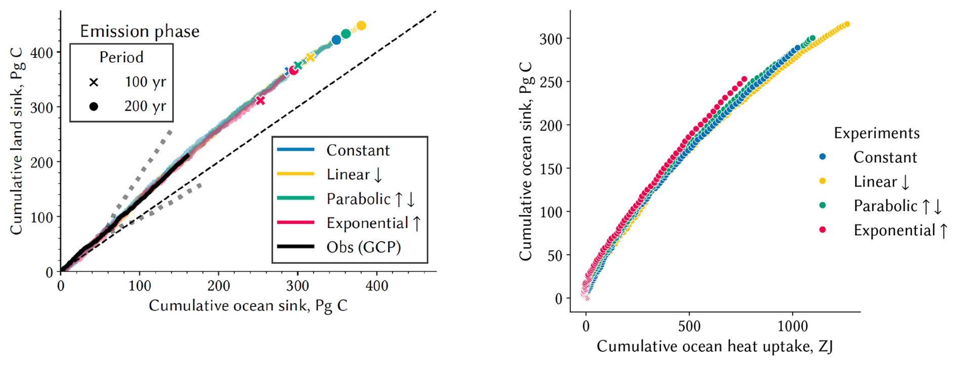
Figure A2 In MPI-ESM simulations with total CO₂ emissions of 1200 Pg C for 100 or 200 years, the sink shares of land versus ocean (left) emerge to keep the same relationship irrespective of pathway profiles. The same is valid for ocean carbon vs. heat uptake (right). For details, see paper by Winkler et al. (2024).

Table A1 List of parameters used in the analysis.

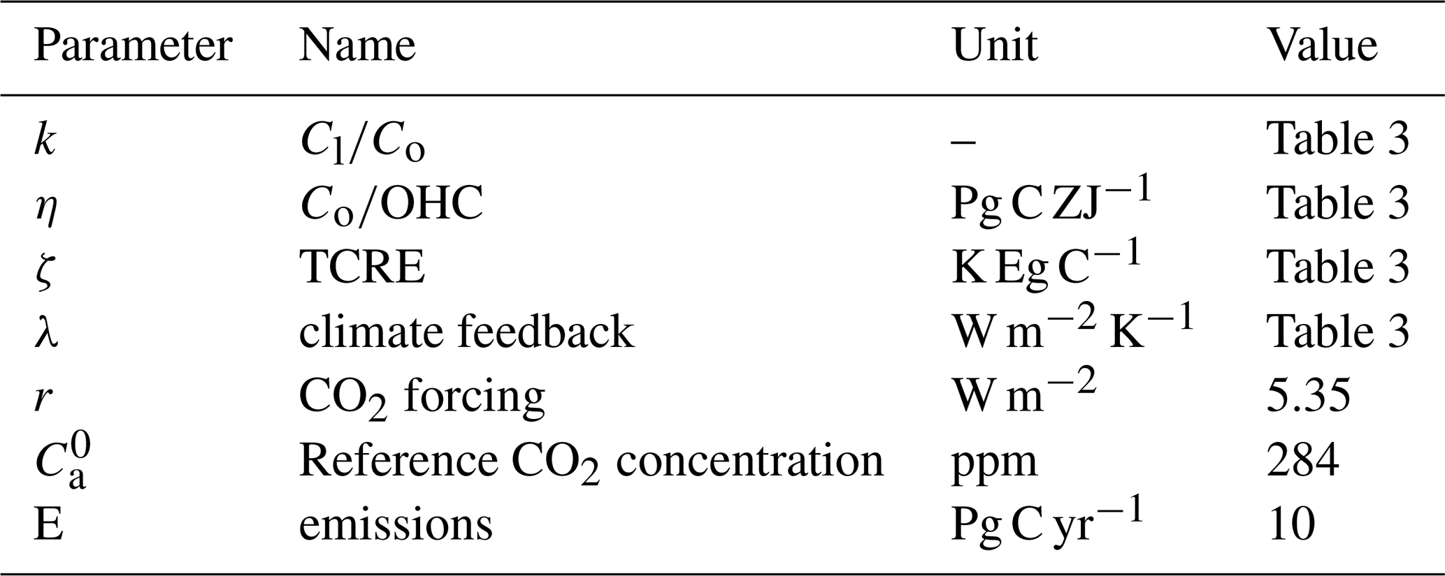
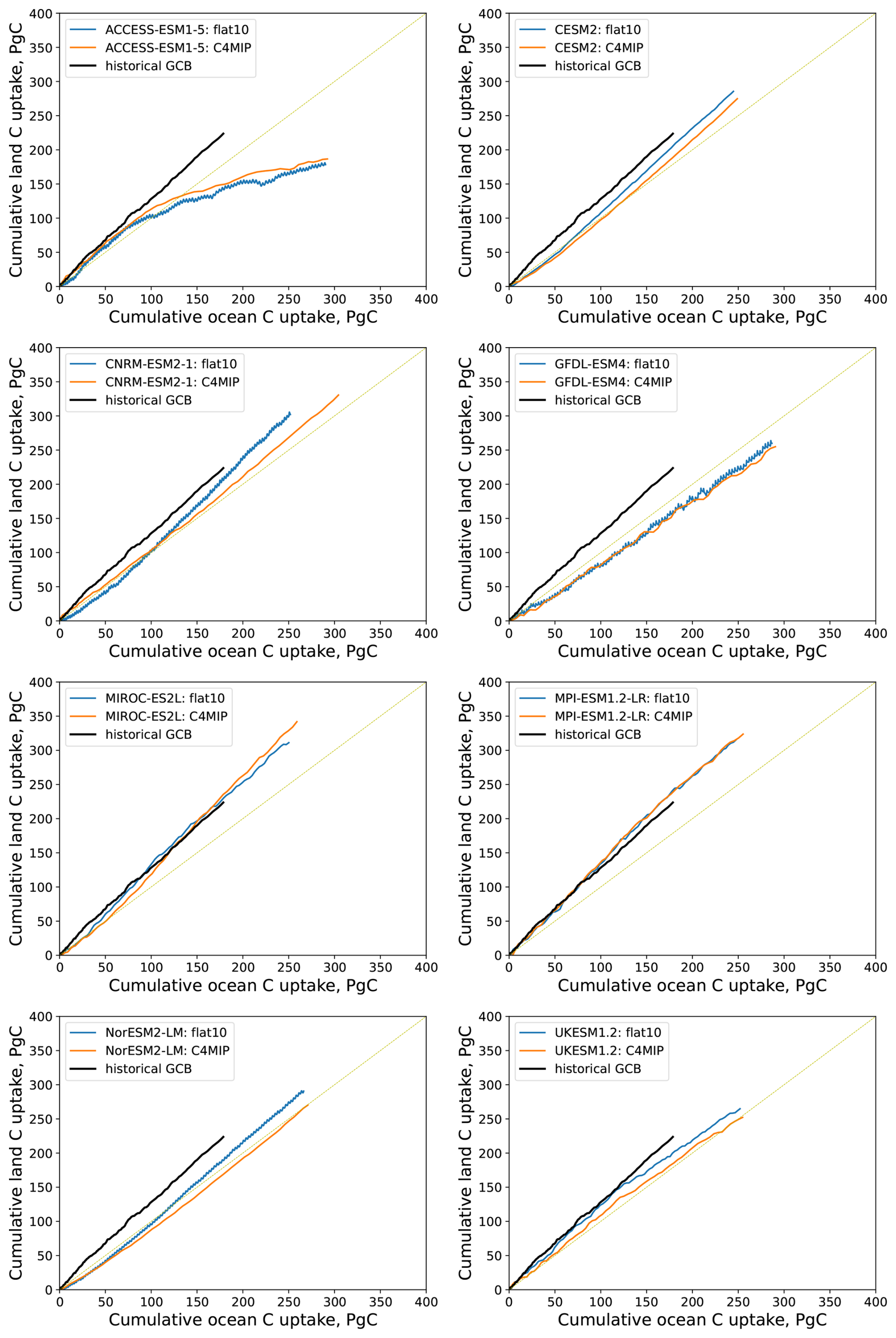
Figure A3 Cumulative land vs. cumulative ocean carbon uptake in the flat10 and C4MIP experiments, data from Arora et al. (2020).