AR6 updates to RF by GHGs and aerosols lowers the probability of accomplishing the Paris Agreement compared to AR5 formulations

We provide a reduced complexity climate model (RCM) evaluation of how the IPCC WG1 Sixth Assessment Report (AR6) updates to the time series of the future atmospheric concentrations of greenhouse gases (GHGs), the effective radiative forcing (ERF) of GHGs, and the ERF of tropospheric aerosols (ERF_AER) affect attributable anthropogenic warming rate, climate sensitivity, and the likelihood of achieving either the target (1.5 °C) or upper limit (2 °C) global warming thresholds of the Paris Agreement (PA). This evaluation is conducted for four selected Shared Socioeconomic Pathway (SSP) scenarios: SSP1–1.9, SSP1–2.6, SSP4–3.4, and SSP2–4.5. Throughout, we compare and contrast these AR6 updates to the state of knowledge that existed prior to the publication of AR6, and provide data-driven probabilistic model simulations based on an evaluation of the impact in the uncertainty of ERF_AER and climate feedback. Our most important findings are that the modeled rate of human-induced warming between 1975 and 2014 is 0.18 (0.13 to 0.21) °C per decade within the AR6 framework (range reflects the 5th and 95th percentiles), which is considerably lower than values found by many Earth system models (ESMs) that participated in Phase 6 of the Coupled Model Intercomparison Project (CMIP6). Effective climate sensitivity (EffCS) inferred from the historical global mean surface temperature (GMST) record was found to be 2.29 (1.54 to 3.11) °C using the ERF datasets from AR6 as model inputs. Upon adoption of the AR6 best estimate for the pattern effect (that is, 0.5 $\mathrm{W}{\mathrm{m}}^{-\mathrm{2}}\mathrm{°}{\mathrm{C}}^{-\mathrm{1}}$), we find values for equilibrium climate sensitivity (ECS) of 3.24 (1.92 to 5.15) °C, which is quite similar to the AR6 assessment of 3.0 (2.0 to 5.0) °C for ECS. The hallmark of our RCM is the ability to conduct large (here, 160 000 member) ensemble forecasts of global warming. These calculations show that AR6 updates to the ERF of GHGs and aerosols result in a considerable decline in the likelihood of limiting warming to either 1.5 or 2 °C of the PA, compared to prior knowledge, for the same future emissions scenarios of GHGs. The likelihood of limiting global warming to 2.0 °C by the end of the century is found to be 100 %, 85 %, 40 %, and 8 % for the SSP1–1.9, SSP1–2.6, SSP4–3.4, and SSP2–4.5 scenarios, respectively, based on the AR6 ERF datasets. Similarly, the ensembles run using the AR6 updates yield likelihoods of 70 %, 32 %, 3 %, and 0 % of limiting warming to 1.5 °C by the end of the century for the same four SSPs. For society to have high confidence in achieving at least the upper limit of 2 °C warming of the PA, the radiative forcing of climate due to GHGs must be placed close to the SSP1–2.6 pathway over the coming decades.

1 Introduction

Reduced complexity models (RCMs) that compute the response of the global mean surface temperature (GMST) to a prescribed radiative forcing (RF) due to anthropogenic greenhouse gases (GHGs) and tropospheric aerosols are becoming increasingly important for evaluating important climate metrics, such as the likelihood of limiting global warming to either the target (1.5 °C) or upper limit (2.0 °C) of the Paris Agreement (PA) (Hope et al., 2017; McBride et al., 2021; Smith et al., 2018a; Nicholls et al., 2020, 2021). There are various types of RCMs, including some with interactive carbon cycles capable of computing atmospheric concentrations of CO₂ and CH₄ from emissions (Meinshausen et al., 2020; Nicholls et al., 2020, 2021). Typically, RCMs represent the global mean energy balance between the atmosphere and the world's oceans on either a monthly or annual timescale, using various types of parameterizations that provide significant computational efficiency compared to three-dimensional Earth system models (ESMs) (Nicholls et al., 2020, 2021). The computational efficiency of RCMs allows for the impact on GMST to be quantified for ensembles with hundreds of thousands of combinations for the RF due to GHGs, aerosols, and climate feedback. Of course, ESMs are essential for providing comprehensive simulations of the changes in the climate system in response to rising anthropogenic RF, such as the spatial distribution of warming, which is a key indicator for the impacts of climate change on local communities (Eyring et al., 2016). Furthermore, ESMs provide a more sophisticated treatment of atmospheric and oceanic interactions than is possible to achieve with RCMs (Nicholls et al., 2020, 2021).

We use a multiple linear regression (MLR) energy balance model, termed the Empirical Model of Global Climate (EM–GC) (Canty et al., 2013; Mascioli et al., 2012; Hope et al., 2017; McBride et al., 2021), to provide data-driven, probabilistic forecasts of GMST. The model is constrained by the Hadley Centre Climatic Research Unit version 5 (HadCRUT5) record for GMST over 1850–2019 (Morice et al., 2021), as described by McBride et al. (2021). In the McBride et al. (2021) paper, their projections of GMST were based on the time series for the atmospheric concentration of GHGs and the RF of tropospheric aerosols from Shared Socioeconomic Pathway (SSP) scenarios published in between the time of the fifth (AR5) Working Group 1 (WG1) Intergovernmental Panel on Climate Change (IPCC) report (IPCC, 2013) and the sixth (AR6) WG1 IPCC report (IPCC, 2021c). We had used formulations for the RF of GHGs from AR5 in McBride et al. (2021). Here, we rely upon formulations for the RF of GHGs given in AR6, which as detailed in Sect. 2.1.2 differ from the earlier formulations due to several new considerations within AR6. Similarly, we rely on updated time series of the atmospheric concentrations of GHGs given in AR6 for four selected SSP scenarios (that is, SSP1–1.9, SSP1–2.6, SSP4–3.4, and SSP2–4.5), which also differ from the pre-AR6 time series of GHGs due to the use of an updated model to compute atmospheric concentrations from prescribed emissions (Sect. 2.1.1). Finally, we use the AR6 update for the RF due to tropospheric aerosols, which also differs considerably from the AR5-based values used by McBride et al. (2021) (Sect. 2.1.3). The projections of GMST shown throughout this paper are motivated by quantifying the likelihood of achieving either the target (1.5 °C) or upper limit (2.0 °C) of global warming under the PA for various assumptions regarding GHGs and aerosols.

Section 2 provides a brief overview of the EM–GC model. Section 3 describes the simulations of GMST, the attributable anthropogenic warming rate, climate sensitivity and global warming projections found using our reduced complexity model. Throughout, we focus on comparing results found using the model inputs of McBride et al. (2021) (that is, the pre-AR6 estimates termed “Baseline simulations”) with results found using the AR6 values of the model inputs. We show that considerable differences are found for the end-of-century GMST and the probability of achieving either the target (1.5 °C) or upper limit (2.0 °C) of the Paris Agreement, between the Baseline and the AR6 values for model inputs, despite the fact that, for any given SSP scenario, both formulations are based on the same time series of GHG emissions (Sect. 3.2). We conclude by comparing our GMST projections to output from ESMs that participated in Phase 6 of the Coupled Model Intercomparison Project (CMIP6) (Eyring et al., 2016). A brief set of concluding remarks is given in Sect. 4.

Table 1 Data sources for the Baseline and AR6 framework simulations.

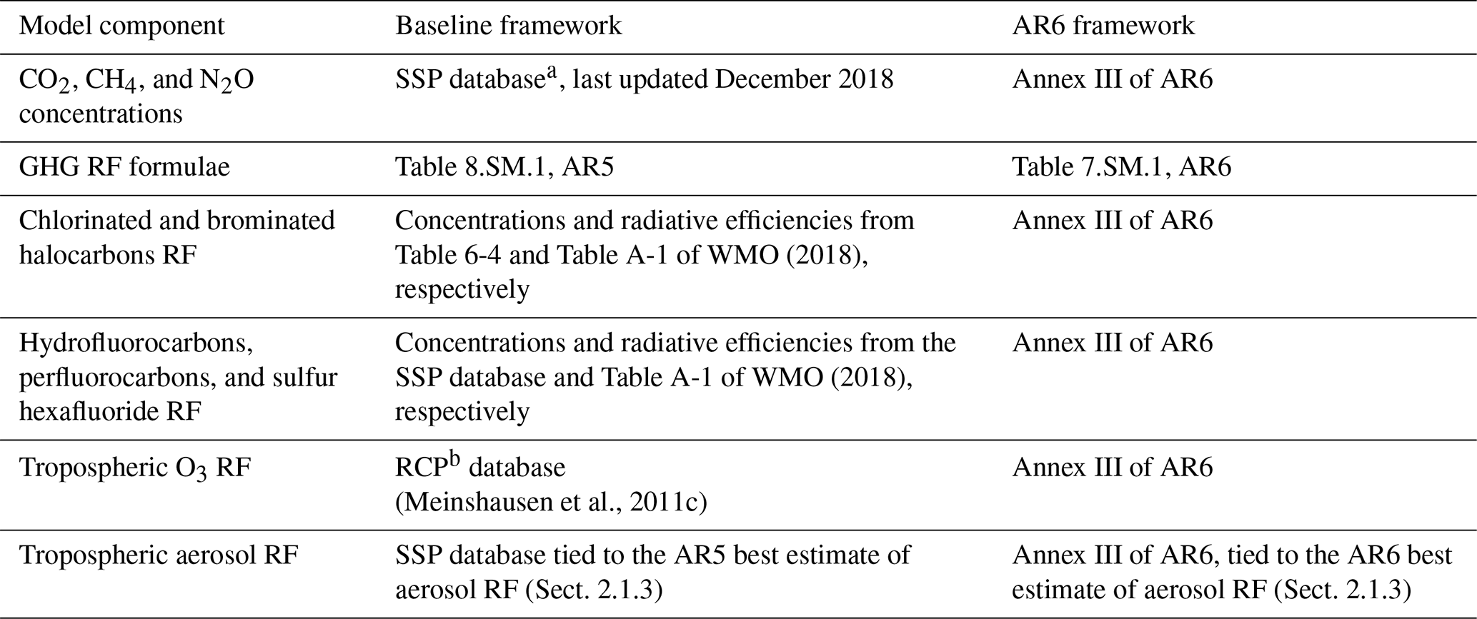
^a SSP database: https://tntcat.iiasa.ac.at/SspDb/dsd (last access: 17 February 2020). ^b RCP: Representative Concentration Pathways.

2 Data and methods

Our EM–GC is designed to quantify the influence of a variety of anthropogenic and natural influences on GMST, using a MLR energy balance approach. The anthropogenic contribution to GMST is simulated by the energy balance component of the model from the radiative forcing due to GHGs, tropospheric aerosols, and land use change (LUC), while also accounting for the export of heat from the atmosphere to the world's oceans (ocean heat export or OHE). The MLR component of the model is responsible for quantifying the influence of various natural factors on the GMST in a manner similar to other MLR-based analyses of the climate system (Lean and Rind, 2008, 2009; Foster and Rahmstorf, 2011; Zhou and Tung, 2013). Natural factors include increases in stratospheric aerosols due to major volcanic eruptions, the approximate 11-year variation in total solar irradiance (TSI), as well as interactions between the ocean and the atmosphere due to the El Niño–Southern Oscillation (ENSO), the Atlantic Meridional Overturning Circulation (AMOC), the Pacific Decadal Oscillation (PDO), and the Indian Ocean Dipole (IOD). The reader is directed towards Sect. 2.1 of McBride et al. (2021) for a more complete description of the model, as well as the governing equations.

Here, we examine four policy-relevant SSP scenarios: SSP1–1.9, SSP1–2.6, SSP2–4.5, and SSP4–3.4 from Tier 1 and Tier 2 of the ScenarioMIP protocol (O'Neill et al., 2016). These were chosen because SSP2–4.5 is the SSP scenario most consistent with recent trends in the anthropogenic emissions of GHGs and aerosols (Meinshausen et al., 2024), while the other three SSPs we have chosen all offer more aggressive means for climate mitigation than the SSP2–4.5 scenario. The second number in the name of the SSP scenario is the target RF at the end of the century (W m⁻²), commonly referred to as the “nameplate RF” (O'Neill et al., 2014). We show model results for two frameworks: a Baseline that represents the state of knowledge prior to AR6 and one that is based on data given in Chap. 7 and Annex III of AR6 (Forster et al., 2021; IPCC, 2021b; Smith et al., 2021a, b).

2.1 Model inputs

Table 1 provides an overview of the source of model inputs for GHG concentrations, the formulae for computing RF due to GHGs, and the RF of tropospheric aerosols in the Baseline and AR6 frameworks. The remainder of this section provides details on various components of this table.

2.1.1 Atmospheric concentrations of greenhouse gases

The EM–GC uses prescribed abundances of GHGs, including CO₂, CH₄, N₂O, tropospheric O₃, chlorinated and/or brominated ozone depleting substances, as well as hydrofluorocarbons, perfluorocarbons, and sulfur hexafluoride, as described in Sect. 2.2.3 of McBride et al. (2021). Here, we focus on describing changes in the atmospheric abundances of CO₂, CH₄, and N₂O that occurred within four SSP scenarios, before and after the publication of AR6, since this change drives the differences central to this study.

Before and after publication of AR6, the atmospheric concentrations of GHGs were computed by other groups using the Model for the Assessment of Greenhouse Gas Induced Climate Change (MAGICC) RCM (Meinshausen et al., 2011a, b, 2020). These times series rely on emissions data from various integrated assessment models (IAMs), as described by Riahi et al. (2017). The Baseline (that is, pre-AR6) projections, which we obtained from the SSP database (Riahi et al., 2017; van Vuuren et al., 2017; Fricko et al., 2017; Fujimori et al., 2017; Calvin et al., 2017; Kriegler et al., 2017; Rogelj et al., 2018), were found using version 6.8 of MAGICC. The AR6 projections, which we obtain from Annex III of AR6 (IPCC, 2021b), are based on model runs with version 7 of MAGICC. MAGICC7 includes important updates relative to MAGICC6.8, such as a permafrost feedback module that results in additional emissions of CO₂ and CH₄ from the thawing of permafrost (Meinshausen et al., 2020).

The top three panels of Fig. S1 in the Supplement compare time series of the concentrations of CO₂, CH₄, and N₂O for the Baseline and AR6 frameworks. All of the GHG projections were found for the same underlying emissions scenarios. The impact of updates to MAGICC7 are modest but noticeable for CO₂, quite small for N₂O, and substantial for CH₄. The MAGICC7 updates result in the atmospheric concentration of CH₄ projected in 2100 to be higher by 180 and 400 ppb for SSP2–4.5 and SSP4–3.4, respectively, compared to the projections provided in the SSP database (Riahi et al., 2017).

2.1.2 Radiative forcing of greenhouse gases

The EM–GC uses as input time series of the RF due to GHGs, computed from time series of the atmospheric abundance of each gas. For the Baseline framework, each RF term is found using parameterizations given in Table 8.SM.1 of the AR5 report (Myhre et al., 2013a), as described in Sect. 2.2.3 of McBride et al. (2021). These AR5 formulations, termed effective radiative forcing (ERF), allow for stratospheric temperature adjustments to the instantaneous RF for many GHGs. The AR5 ERF formulae are based on the analysis by Myhre et al. (1998) of output found using line-by-line models (Edwards, 1992; Myhre and Stordal, 1997), and are identical to those given in the third WG1 IPCC report (IPCC, 2001) as well as the fourth report (IPCC, 2007).

Chapter 7 of the AR6 report introduced two important changes to the parameterizations of ERF due to GHGs (Forster et al., 2021). First, the parameterizations were updated to reflect the spectral overlaps of CO₂ and N₂O, the shortwave RF due to CH₄, and a new representation of the H₂O continuum (Etminan et al., 2016; Meinshausen et al., 2020). Second, the AR6 values of ERF accounts for both stratospheric and tropospheric temperature adjustments (Smith et al., 2018b). Consequently, while AR5 considers stratospheric temperature adjusted RF (SARF) to be equal to ERF, these two quantities differ in the AR6 formulation of RF. The AR5 and AR6 formulae for the ERF due to CO₂, CH₄, and N₂O are given in the Supplement.

The middle row of Fig. S1 compares time series of ERF due to CO₂, CH₄, and N₂O for the Baseline (dotted lines) and AR6 (solid lines) frameworks. The results shown in this middle row reflect the AR6 updates to both the ERF and the future atmospheric abundances of GHGs. Values of ERF are higher in the AR6 framework compared to Baseline, with particularly large increases found for the ERFs of CO₂ and CH₄ for the SSP4–3.4 and SSP2–4.5 scenarios. Finally, Fig. S1h compares ERF due to all GHGs for the Baseline and AR6 frameworks. The largest increase in ERF, among the four SSP scenarios considered, is found for SSP4–3.4 and SSP2–4.5, with end-of-century increases of 0.6 and 1.0 W m⁻², respectively. A similar qualitative conclusion was reached by Fredriksen et al. (2023), who contrasted projections of ERF from CMIP5 models with those from CMIP6 models, and found that CMIP6 models project higher levels of ERF by the end of the century relative to CMIP5 models.

2.1.3 Radiative forcing of tropospheric aerosols

Time series of the RF due to tropospheric aerosols (hereafter, aerosols) is another very important input to the EM–GC. Figure S1g compares the total ERF of aerosols (ERF_AER) for the Baseline and AR6 frameworks, which is the sum of direct cooling by aerosols and the effect of aerosols on clouds (that is, the indirect effect). A summary of the ERF_AER time series for the Baseline framework, which considers a range of aerosol types such as sulfate, dust, organic carbon, black carbon, and biomass burning products, is given in Sect. 2.2.4 of McBride et al. (2021). These time series, published prior to the AR6 report, originate from the Potsdam Institute of Climate Research (PICR) website (https://www.pik-potsdam.de/~mmalte/rcps, last access: 21 May 2024) and are based on future emissions of aerosol precursors in the SSP database (Riahi et al., 2017; van Vuuren et al., 2017; Fricko et al., 2017; Fujimori et al., 2017; Calvin et al., 2017; Kriegler et al., 2017; Rogelj et al., 2018).

Considerably stronger aerosol cooling is evident in the AR6 time series of ERF_AER, compared to the Baseline time series (Fig. S1g). Further, the temporal evolution (that is, the shape) of the historical cooling differs substantially between the AR6 and Baseline. Finally, AR5 and AR6 each provide best estimates, and possible ranges for ERF_AER, over the time periods 1750–2011 and 1750–2019, respectively. These estimates were assessed to be −0.9 W m⁻² with a possible range of −0.1 to −1.9 W m⁻² in AR5 (Myhre et al., 2013b), and to be −1.1 (−0.4 to −1.7) W m⁻² in AR6 (Forster et al., 2021). Formally, the possible range limits correspond to the 5th and 95th percentiles.

It is beyond the scope of this paper to delve deeply into the cause of the differences between the AR5 and AR6 estimates of ERF_AER. It is somewhat surprising that the AR6 update to the best estimate of ERF_AER in the year 2019 exhibits more cooling than the AR5 best estimate that reflected conditions out to 2011, because individual time series of ERF_AER in both AR5 and AR6 (Fig. S1g) exhibit a considerable decline in the absolute value of ERF_AER over the 2011–2019 period of time. This decline was driven by successful efforts to reduce the emissions of aerosol precursors, by various entities throughout the world, due to the public health concerns of aerosols (Smith and Bond, 2014; Fu et al., 2021). The primary reason for larger aerosol cooling in the AR6 best estimate of ERF_AER, despite the 8-year extension in end year, is the nearly factor of 2 increase in the assessed value of cooling due to the aerosol indirect effect from AR5's best estimate of −0.45 (0.0 to −1.2) W m⁻² to the AR6 best estimate of −0.84 (−0.25 to −1.45) W m⁻². A significant decline in the best estimate of black carbon warming in AR6 (0.11 (−0.20 to 0.42) W m⁻²) compared to AR5 (0.4 W m⁻² (0.05 to 0.80) W m⁻²) also contributes to the decline in the absolute value of ERF_AER in AR6, compared to AR5. There are other updates in the AR6 approach for ERF_AER, as summarized in Sect. 7.3.3 of Forster et al. (2021).

Recently, Zelinka et al. (2023) pointed out two coding errors in the Smith et al. (2020) paper that influenced the AR6 evaluation of ERF_AER. These two errors largely cancel for the evaluation of ERF_AER. The Zelinka et al. (2023) best estimate and standard deviation of ERF_AER, over 1750 to 2014, is −1.09 ± 0.24 W m⁻², which is slightly less aerosol cooling than the AR6 estimate of −1.3 (−0.6 to −2.0) W m⁻² for the same time period. Given the “medium confidence” associated with the assessed value of ERF_AER noted in Chap. 7 of AR6 (Forster et al., 2021), the lack of evaluation of ERF_AER by Zelinka et al. (2023) for the 1750 to 2019 time period that is central to our study, and the focus within Zelinka et al. (2023) on the evaluation of the various components of ERF_AER for contemporary periods of time rather than the historical evolution of ERF_AER, we have decided to use the AR6 historical time series for aerosol cooling as presented in the assessment.

Time series of ERF_AER are vitally important inputs to the EM–GC. A hallmark of this approach is spanning a wide range of possible time series of ERF_AER as well as a model parameter λ_Σ that represents the sum of all climate feedbacks, retaining for further analysis the members of this ensemble that satisfy three goodness-of-fit constraints on the observed (1) 170-year GMST record, (2) GMST record over the past 8 decades (formally, 1940 to 2019), and (3) ocean heat content record that begins in 1955. Further details of this ensemble approach are given in Sect. 2.1 of McBride et al. (2021). Figure S2 in the Supplement illustrates the approach for generating an ensemble of ERF_AER time series for the SSP2–4.5 scenario, within the AR6 framework. The solid black line shows the AR6 assessed best value of the time series of ERF_AER. An ensemble is created by scaling this time series by various constant multiplicative factors, with the color scheme chosen to highlight the numerical value of ERF_AER in 2019. A similar approach is used for the Baseline framework, relying upon time series of ERF_AER obtained from the aforementioned PICR website, as detailed in Sect. 2.5 and Fig. S7 of McBride et al. (2021). While one can envision a more sophisticated approach that allows for the alteration of the shape of ERF_AER, in addition to the magnitude, the actual ERF_AER responds quickly to changes in precursor emissions due to the short lifetime of tropospheric aerosols. Generally, historical aerosol precursor emissions are fairly well known (e.g., Hoesly et al., 2018). The more sophisticated approach of Smith and Bond (2014), which relied upon a RF parameterization tied to the emission of sulfate, black carbon, and organic carbon aerosols, resulted in an ensemble of time series for ERF_AER that exhibit nearly the same shape, with quite different peak cooling.

Figure S1i shows time series of total anthropogenic ERF (ERF_ANTH). As noted above, the design of the SSPs was predicated on the end-of-century RF due to all human activity being close to the last numerical value in the scenario (that is, 4.5 W m⁻² for SSP2–4.5) (O'Neill et al., 2014; Tebaldi et al., 2021). Close agreement of end-of-century ERF_ANTH and the SSP nameplate is found using GHG concentrations together with ERF formulations for the Baseline framework. Conversely, within the AR6 framework, ERF_ANTH in 2100 exceeds the nameplate values, with the difference being particularly large for SSP4–3.4 (0.6 W m⁻²) and SSP2–4.5 (0.9 W m⁻²). One final, important difference between the two frameworks is the steeper rise in ERF_ANTH between about 1960 and present within AR6 compared to Baseline, which is attributable to an assessed best value of much stronger aerosol cooling over the latter part of the prior century in AR6 relative to the Baseline (Fig. S1g).

2.1.4 Other model inputs

The EM–GC output shown below relies entirely on simulations that we constrain to match the HadCRUT5 GMST anomaly (ΔT) record (Morice et al., 2021) over the years 1850–2019. Model simulations are also constrained by observations of Ocean Heat Content (OHC) that start in 1955. Here, we use the average OHC from data provided by five groups: Levitus et al. (2012), Balmaseda et al. (2013), Cheng et al. (2017), Ishii et al. (2017), and Carton et al. (2018). Further details, including the evaluation of the uncertainties in observed ΔT and OHC, are given in Sect. 2.2 of McBride et al. (2021).

The EM–GC simulations consider a variety of natural factors alongside the anthropogenic component of warming. The ENSO time series used during the training period (1850–2019) is based on Version 2 of the Multivariate ENSO Index (MEI.v2) (Wolter and Timlin, 1993; Zhang et al., 2019). The MEI.v2 dataset provides data starting in 1979. For 1850 to 1978, a historical extension based on Wolter and Timlin (2011) and the HadSST3 dataset (Kennedy et al., 2011) is used, as detailed in Sect. 2.2.6 of McBride et al. (2021). The input time series that is used to reflect changes in the strength of the AMOC is based on sea surface temperature (SST) data from HadSST4 (Kennedy et al., 2019) between the Equator and 60° N in the Atlantic Ocean, detrended using the magnitude of global anthropogenic radiative forcing, then Fourier-filtered to remove frequencies above $\mathrm{1}/\mathrm{9}$ years⁻¹ as described in Sects. 3.2.3 and 4.1.2 of Canty et al. (2013), as well as Sect. 2.2.7 of McBride et al. (2021). Input time series for the PDO and the IOD, which are found to have little effect on the historical simulations of ΔT, are the same as described by McBride et al. (2021). Indices for all of the oceanic proxies after 2019, which marks the end of the training period, are set to zero.

The model also considers the impact on ΔT of variations in total solar irradiance (TSI) and major volcanic eruptions. The input time series for TSI anomalies is constructed from CMIP6 model data between 1850 and 2014 (Matthes et al., 2017), while values for 2015–2019 are obtained from the Solar Radiation and Climate Experiment (SORCE) (Dudok de Wit et al., 2017). The input time series for stratospheric aerosol optical depth (SAOD), for 1850 to 1978, is based on extinction coefficients obtained from the Volcanic Forcing Dataset (Arfeuille et al., 2014) that had been prepared for CMIP6 ESM runs. For 1979 to 2018, we use a time series of SAOD at 550 nm from the Global Space-based Stratospheric Aerosol Climatology (GloSSAC v2.0) (Thomason et al., 2018). For the earlier time period (1850 to 1978), the extinction coefficients from the Volcanic Forcing Dataset were integrated from the tropopause to 39.5 km, to obtain a globally averaged SAOD, weighted by the cosine of latitude from 80° S to 80° N. For the latter time period (1979 to 2018), we calculate globally averaged SAOD from the GloSSAC dataset using cosine-latitude weighting over the same range of latitudes. For the year 2019, level 3 gridded SAOD product from the Cloud-Aerosol Lidar and Infrared Pathfinder Satellite Observations (CALIPSO) (Vaughan et al., 2004) is used to obtain a global average SAOD, which is then offset by the average difference between the GloSSAC and CALIPSO datasets for the period of overlap (2006–2018) between the two datasets, as described in Sect. 2.2.5 of McBride et al. (2021). Values of the TSI anomaly beyond 2019 are set to zero, while for SAOD we use the value from December 2019 for 2020 to 2100. The input time series for all natural and anthropogenic factors are archived in Zenodo (Farago et al., 2025).

2.2 Model outputs

Here we provide a brief overview of various outputs of the EM–GC simulations that will be described in Sect. 3.

2.2.1 Attributable anthropogenic warming rate and effective climate sensitivity

Attributable anthropogenic warming rate (AAWR) is defined as the rate of change of the GMST anomaly (ΔT) due to anthropogenic activity, between 1975 and 2014. This time interval spans a 40-year period in which ΔT rose in a near-linear manner due to human activity (McBride et al., 2021). AAWR is determined as the slope of a linear fit to the anthropogenic component of global warming, defined by Eq. (9) of McBride et al. (2021). This method for the evaluation of AAWR is similar to earlier, MLR-based studies (Lean and Rind, 2008, 2009; Foster and Rahmstorf, 2011; Zhou and Tung, 2013), except that we quantitatively account for the impact of the uncertainty in the RF of aerosols and the strength of climate feedback on the possible range of AAWR.

Equilibrium climate sensitivity (ECS) is defined as the rise in ΔT after climate has equilibrated to a theoretical doubling of the pre-industrial concentration of CO₂ (IPCC, 2001, 2021a; Forster et al., 2021). Since equilibrium can take centuries to reach due to the slow transfer of heat to the deep oceans (Hansen et al., 2011; Church et al., 2013; Tokarska et al., 2020a), often the more short-term effective climate sensitivity (EffCS) is used (Gregory et al., 2020; Tokarska et al., 2020a; Spencer and Christy, 2023). We compute EffCS from the ERF due to the doubling of the pre-industrial CO₂ concentration ($\mathrm{\Delta }{\mathrm{ERF}}_{\mathrm{2}\times {\mathrm{CO}}_{\mathrm{2}}}$) as shown in Eq. (1),

$$\begin{array}{}\text{(1)}& \text{EffCS}={\displaystyle \frac{\mathrm{1}}{{\mathit{\lambda }}_{\mathrm{p}}-{\mathit{\lambda }}_{\mathrm{\Sigma }}}}\times \mathrm{\Delta }{\mathrm{ERF}}_{\mathrm{2}\times {\mathrm{CO}}_{\mathrm{2}}},\end{array}$$

where λ_p is a constant equal to 3.2 $\mathrm{W}{\mathrm{m}}^{-\mathrm{2}}\mathrm{°}{\mathrm{C}}^{-\mathrm{1}}$, λ_Σ represents the sum of all feedbacks that varies for different members of the ensemble, and $\mathrm{\Delta }{\mathrm{ERF}}_{\mathrm{2}\times {\mathrm{CO}}_{\mathrm{2}}}$ is the rise in RF due to a doubling of CO₂. This methodology, based on the terminology of Bony et al. (2006), is consistent with Box 7.1 of AR6 (Forster et al., 2021). Within the Baseline framework, we use the RF formula of Myhre et al. (1998), which leads to $\mathrm{\Delta }{\mathrm{ERF}}_{\mathrm{2}\times {\mathrm{CO}}_{\mathrm{2}}}$ = 5.35×ln (2) = 3.71 Wm⁻². For the AR6 framework, we use a value for $\mathrm{\Delta }{\mathrm{ERF}}_{\mathrm{2}\times {\mathrm{CO}}_{\mathrm{2}}}$ of 3.93 W m⁻², which is the best estimate for $\mathrm{\Delta }{\mathrm{ERF}}_{\mathrm{2}\times {\mathrm{CO}}_{\mathrm{2}}}$ given in Sects. 7.3.2.1 and 7.SM.1.2 of AR6 (Forster et al., 2021; Smith et al., 2021a). Consequently, EffCS computed using the AR6 formula is 6 % larger than that found using the Myhre et al. (1998) formula for a given value of λ_Σ. Finally, we note that climate sensitivity deduced from historical warming may be different from true ECS, as the historical climate feedback could differ from the climate feedback under an abrupt 4 × CO₂ forcing scenario that is often used to evaluate ECS in ESMs (Andrews et al., 2018; Andrews et al., 2019; Winton et al., 2020; Forster et al., 2021).

2.2.2 Future temperature projections

Projections of ΔT, for various SSP scenarios, are central to assessing the likelihood of achieving either the Paris Agreement target (1.5 °C) or upper limit (2.0 °C) for the rise of GMST relative to pre-industrial (Hope et al., 2017; McBride et al., 2021; Smith et al., 2018a; Nicholls et al., 2020, 2021). An important aspect of EM–GC simulations is the ability to compute probabilistic forecasts of the rise in ΔT, taking into account the uncertainty in the radiative forcing of climate due to tropospheric aerosols.

To consider the uncertainty in the magnitude of net climate feedback and the strength of aerosol cooling, we use a 160 000 member ensemble, comprised of 400 possible values for the parameter λ_Σ, each combined with 400 time series for ERF_AER. This ensemble serves as the basis for the probabilistic forecasts of ΔT, as well as the numerical evaluations of AAWR and EffCS. We consider only the members of the ensemble that satisfy three χ²-based metrics given by Eqs. (S1)–(S3) in the Supplement (that is, each χ² value must be ≤ 2), which serve as the observational constraints of the model. Two of these metrics quantify how well the modeled GMST anomaly represents the observed temperature anomaly of the atmosphere for the entire training period (1850–2019, ${\mathit{\chi }}_{\text{ATM}}^{\mathrm{2}}$) and over the last 80 years (1940–2019, ${\mathit{\chi }}_{\text{RECENT}}^{\mathrm{2}}$). The third metric (${\mathit{\chi }}_{\text{OCEAN}}^{\mathrm{2}}$) is a goodness-of-fit value between the observed and modeled ocean heat content. The ${\mathit{\chi }}_{\text{RECENT}}^{\mathrm{2}}$ metric is used because without this particular constraint, some solutions with values of ${\mathit{\chi }}_{\text{ATM}}^{\mathrm{2}}\le$ 2 have a visually poor simulation of the observed rise in GMST over the past 4 to 5 decades, due to the large uncertainty associated with early measurements of ΔT, as described in Sect. 2.1 of McBride et al. (2021).

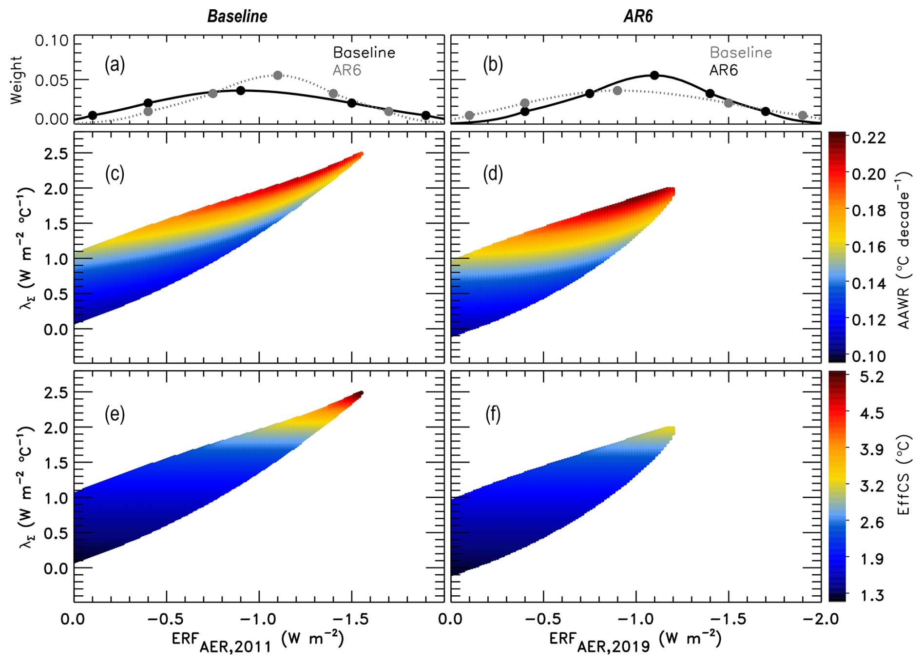
Figure 1 Aerosol weighting method and EM–GC-computed values of AAWR and EffCS for combinations of ERF_AER and λ_Σ. (a, c, e) Simulations using the Baseline framework. (b, d, f) Simulations using the AR6 framework. (a, b) Asymmetrical Gaussians used to weight aerosol scenarios for probabilistic forecasts, as described in Sect. 2.2.2. Points marked on the Gaussians represent specific ERF values used as the central values, as well as 1σ and 2σ boundaries of each Gaussian (Table S3). The Gaussians are overlaid for visual comparison. The Gaussians shown with the solid black line are used to weight the EM–GC output in each column. (c, d) EM–GC-computed values of AAWR for the λ_Σ–ERF_AER ensemble. Colors denote the specific values of AAWR as indicated by the color bar on the right and are only shown for the combinations of ERF_AER and λ_Σ for which a good fit to the HadCRUT5 historical climate record was found. (e, f) EM–GC-computed values of EffCS for the λ_Σ–ERF_AER ensemble.

For the results shown in Sect. 3, the observationally constrained ensemble is then weighted by an asymmetrical Gaussian function, shown in Fig. 1a and b, centered around the IPCC best estimate of ERF_AER in the reference year (−0.9 W m⁻² in 2011 for the Baseline framework and −1.1 W m⁻² in 2019 for the AR6 framework). The 1σ and 2σ boundaries of the Gaussians are derived from the possible and likely ranges for ERF_AER provided by the AR5 (Baseline framework) and AR6 (AR6 framework) reports (Table S3 in the Supplement). The Gaussians are asymmetrical because the likely and possible ranges of ERF_AER specified in AR5 and AR6 are not symmetric around the respective best estimates. The weighted ensemble is then used to compute probabilistic estimates of AAWR and EffCS (Sect. 3.1), as well as probabilistic forecasts on the GMST anomaly (Sect. 3.2).

The projections of ΔT shown in Sect. 3 assume that the climate feedback parameter, λ_Σ, is constant over time. Support for this assumption is given by the temporal invariance of the residual between measured and modeled values of ΔT, over the past century and a half, as shown in Fig. 14 of McBride et al. (2021). If the true value of λ_Σ varies over time, as has been suggested based on analysis of CMIP5 (Marvel et al., 2018; Rugenstein et al., 2020) and CMIP6 (Dong et al., 2020; Salvi et al., 2023), then the analysis conducted by McBride et al. (2021) indicates that the end-of-century projections of global warming could be biased low by a few tenths of degrees Celsius. Regardless, the primary contributor to the uncertainty in end-of-century warming is the imprecise knowledge of ERF_AER.

3 Results

3.1 Attributable anthropogenic warming rate and effective climate sensitivity

We begin by analyzing values of AAWR found from the EM–GC ensemble simulation of ΔT over the 1850 to 2019 time period. As noted above, our estimates of AAWR quantify the human contribution to the rate of global warming from 1975 to 2014. Figure 1 shows the values of AAWR (Fig. 1c and d) and EffCS (Fig. 1e and f), as the function of climate feedback (vertical axis) and the strength of aerosol cooling (horizontal axis) for the Baseline (Fig. 1a, c, and e) and AR6 frameworks (Fig. 1b d, and f). Colors corresponding to values of AAWR and EffCS are only shown for combinations of λ_Σ and ERF_AER for which a good fit to the historical GMST and OHC record was obtained, defined by the values of all three reduced χ² indicators being ≤ 2. Figure 1a and b show the asymmetrical Gaussian functions used to weight the EM–GC output described in Sect. 2.2.2. Notably, the highest values of λ_Σ for which the model can achieve a good fit to the historical climate record is lower for the AR6 framework relative to Baseline, which allows for a tighter constraint on the upper limit of EffCS. This difference is driven by the considerable variation in the shape of the best estimate of the ERF_AER associated with each framework (Fig. S1g) that drives considerable variations in the value of total anthropogenic ERF between about 1960 and 2000 (Fig. S1i).

The weighted median estimate and 5 %–95 % range for AAWR are 0.16 (0.12 to 0.20) and 0.18 (0.13 to 0.21) °C per decade for the Baseline and AR6 frameworks, respectively. The probability distribution function (PDF) of AAWR, for both frameworks, is shown in Fig. S3a in the Supplement. The estimates of AAWR are quite similar for the two frameworks, which is of course to be expected since both estimates result from observations of the GMST anomaly that are identical for both sets of ensembles. The slightly higher median value of AAWR in the AR6 framework is due to a larger slope of ERF_ANTH over 1975 to 2014, 0.47 W m⁻² per decade, compared to the 0.36 W m⁻² per decade slope of ERF_ANTH in the Baseline framework. The values of AAWR within both frameworks are considerably lower than the median and 5 %–95 % range of 0.221 (0.151 to 0.299) °C per decade from the CMIP6 multi-model ensemble derived by McBride et al. (2021). This finding is consistent with Samset et al. (2023), who found that “virtually all CMIP6 simulations have higher 50-year warming rates than the observations”, using an ensemble of 119 ESM simulations from CMIP6. The empirical estimates of AAWR align well with several other recent empirical estimates, suggesting that our quantification of the natural and anthropogenic drivers of the variations in ΔT is consistent with other studies. Recent estimates of AAWR are between 0.17 to 0.20 °C per decade based on the 1973–2022 period (Samset et al., 2023) and the 1980–2020 period (Table 2.4 of AR6 Chap. 2; Gulev et al., 2021; Forster et al., 2023). Finally, the rate of warming has likely accelerated since 1990 at a rate of 0.008 to 0.025 °C decade⁻¹ per decade (Samset et al., 2023), with Forster et al. (2023) finding a rate of 0.2 °C per decade for human-induced warming for the 2013–2022 period, while Ribes et al. (2021) found this rate to be 0.23 °C per decade over the 2010–2019 period.

Figure 1e and f show values of EffCS obtained for the Baseline and AR6 frameworks. The median EffCS is nearly identical for the Baseline and AR6 frameworks, at 2.26 and 2.29 °C, respectively. However, the corresponding 5 %–95 % ranges of EffCS differ considerably, with the Baseline range of (1.45 to 4.37) °C being considerably larger than that found using the AR6 framework (1.54 to 3.11) °C. This difference is readily apparent in the PDFs of EffCS for both frameworks, as shown in Fig. S3b. Simulations based on the AR6 framework allow for a tighter constraining of the upper estimate of EffCS, due to the fact that within this ensemble, we are not able to obtain good fits to the historical GMST and OHC records with values of λ_Σ greater than about 2.0 $\mathrm{W}{\mathrm{m}}^{-\mathrm{2}}\mathrm{°}{\mathrm{C}}^{-\mathrm{1}}$. In contrast, simulations in the Baseline framework can achieve good fits for stronger levels of climate feedback, upwards to about 2.5 $\mathrm{W}{\mathrm{m}}^{-\mathrm{2}}\mathrm{°}{\mathrm{C}}^{-\mathrm{1}}$, that also correspond to higher amounts of aerosol cooling (Fig. 1e and f). Our estimate for EffCS of 2.29 (1.54 to 3.11) °C within the AR6 framework exhibits close agreement with the results of Skeie et al. (2024), who found the best estimate and 90 % uncertainty range for EffCS to be 2.2 (1.6 to 3.0) °C using a Bayesian estimation model and ERF datasets from AR6, while assuming climate feedback to be constant over the historical period, similar to our approach.

We now discuss the relationship between the estimates of EffCS from our model simulations and ECS. Values of ECS can be approximated from observationally constrained estimates of EffCS by applying a correction factor to the strength of the climate feedback term, termed α^′, as shown in Eq. (2). Here, α^′ represents the difference between climate feedback inferred from historical warming and the climate feedback consistent with an equilibrated climate following an abrupt doubling of the pre-industrial concentrations of CO₂ (hereafter abrupt2xCO₂), as described in Sects. 7.4.4.3 and 7.5.2 of Forster et al. (2021). This difference in climate feedback is associated with differences in the spatial pattern of warming over the historical period and the equilibrium warming pattern, termed the pattern effect.

$$\begin{array}{}\text{(2)}& \text{ECS}={\displaystyle \frac{\mathrm{1}}{{\mathit{\lambda }}_{\mathrm{p}}-{\mathit{\lambda }}_{\mathrm{\Sigma }}-{\mathit{\alpha }}^{\prime }}}\times \mathrm{\Delta }{\mathrm{ERF}}_{\mathrm{2}\times {\mathrm{CO}}_{\mathrm{2}}}\end{array}$$

Section 7.4.4.3 of AR6 assessed α^′ to have a value of 0.5 ± 0.5 $\mathrm{W}{\mathrm{m}}^{-\mathrm{2}}\mathrm{°}{\mathrm{C}}^{-\mathrm{1}}$, at a low confidence level. The large uncertainty is due to the fact that estimates for the value of α^′ vary greatly between individual studies and specific CMIP models (Armour, 2017; Proistosescu and Huybers, 2017; Andrews et al., 2018; Andrews et al., 2019; Dong et al., 2020; Winton et al., 2020). The black symbols in Fig. 2 show ECS found using Eq. (2) as a function of the value of α^′ for the AR6 ensemble EM–GC simulation. The dots and error bars represent the median and 5 %–95 % range of ECS, respectively. The green dashed line and shaded area correspond to the central value and very likely range of ECS given in Table 7.13 of the AR6 report (Forster et al., 2021).

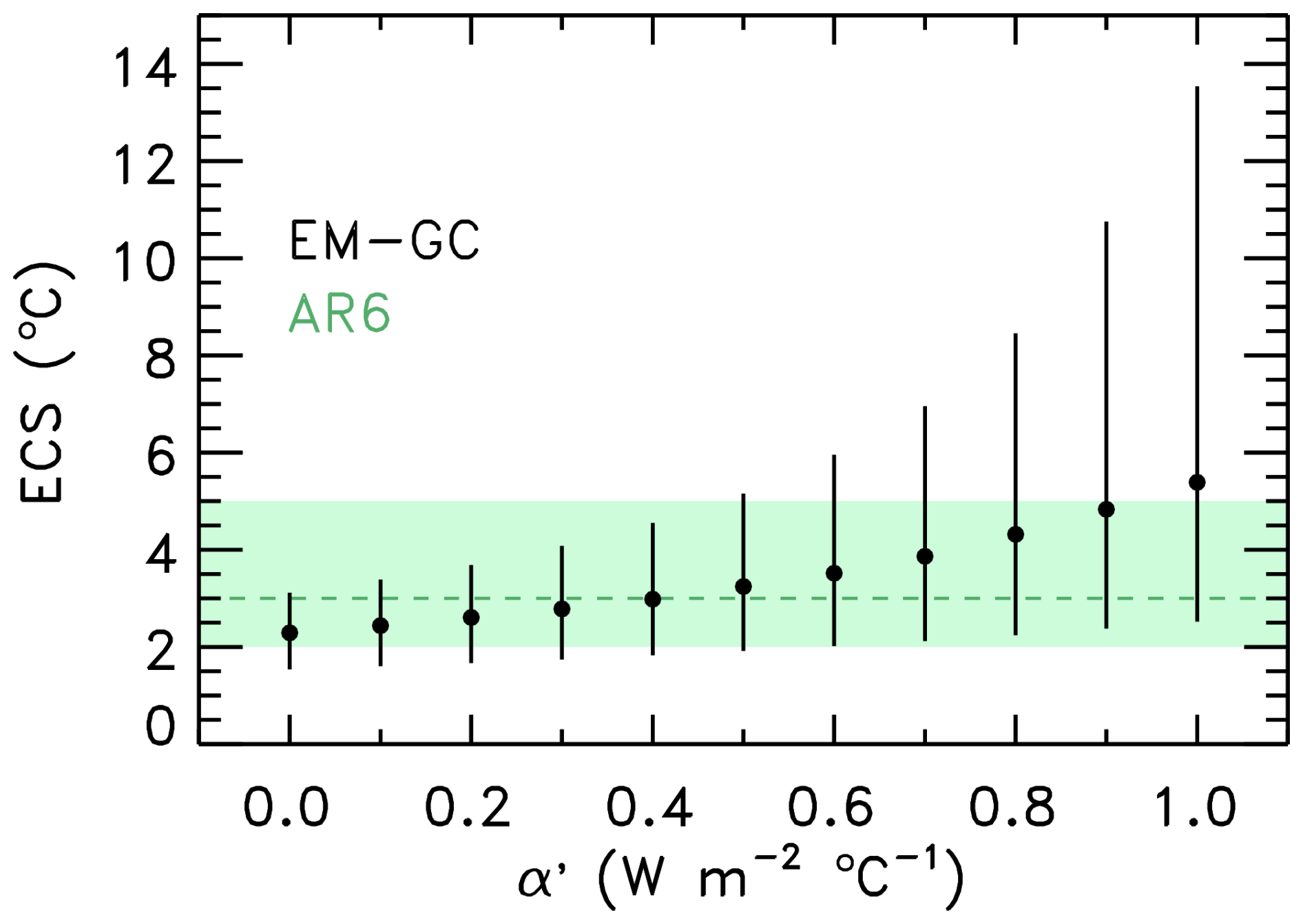
Figure 2 Equilibrium climate sensitivity (ECS) as the function of the pattern effect (α^′, see text). Black vertical bars and circles correspond to the EM–GC 5 %–95 % range, and 50 % probability, respectively. The green shaded area and horizontal dashed line represent the AR6 very likely range, and central estimate of ECS, respectively, from Table 7.13 of Forster et al. (2021). All results shown in this figure are based on simulations that use inputs from the AR6 framework.

For α^′ = 0 $\mathrm{W}{\mathrm{m}}^{-\mathrm{2}}\mathrm{°}{\mathrm{C}}^{-\mathrm{1}}$ (corresponding to no pattern effect), EffCS is equal to ECS and we obtain the median and range for ECS of 2.29 (1.54 to 3.11) °C, which had been given above. For the AR6 best estimate of α^′ = 0.5 $\mathrm{W}{\mathrm{m}}^{-\mathrm{2}}\mathrm{°}{\mathrm{C}}^{-\mathrm{1}}$, we find ECS to be 3.24 (1.92 to 5.15) °C, which is in very good agreement with the AR6 assessment of ECS (green shaded region). The AR6-based upper limit of α^′ = 1.0 $\mathrm{W}{\mathrm{m}}^{-\mathrm{2}}\mathrm{°}{\mathrm{C}}^{-\mathrm{1}}$ yields a median and 5 %–95 % range of 5.39 (2.52 to 13.54) °C, which tends to exceed the assessed value of ECS from AR6. These results highlight the sensitivity of ECS to the pattern effect, a concept first introduced in the latest WG1 IPCC report. The value of ECS found here for α^′ = 0.5 $\mathrm{W}{\mathrm{m}}^{-\mathrm{2}}\mathrm{°}{\mathrm{C}}^{-\mathrm{1}}$ is consistent with Skeie et al. (2024), who performed a similar analysis and found their estimate of ECS to be “almost identical” to the AR6 central value and very likely range of 3.0 (2.0 to 5.0) °C, upon using the AR6 best estimate for the value of α^′. Finally, our estimates of ECS for α^′ = 0.5 $\mathrm{W}{\mathrm{m}}^{-\mathrm{2}}\mathrm{°}{\mathrm{C}}^{-\mathrm{1}}$ also show good consistency with the range for ECS of 2.42 to 5.83 °C obtained from millennium-long CMIP model simulations (Rugenstein et al., 2020) performed under the auspices of the LongRunMIP protocol (Rugenstein et al., 2019).

Figure 2 shows that the 5th percentile values of ECS vary between about 1.5 and 2.5 °C depending on the magnitude of α^′, consistent with the AR6 assessment of ECS being greater than 1.5 °C at a virtually certain level of confidence (Forster et al., 2021). Further, the 50th percentile estimates for ECS (black dots) fall into the range of ECS assessed by AR6 (green shading), except for α^′ = 1.0 $\mathrm{W}{\mathrm{m}}^{-\mathrm{2}}\mathrm{°}{\mathrm{C}}^{-\mathrm{1}}$. Conversely, the 95th percentile estimates for ECS vary greatly with α^′, and exhibit a substantially larger level of variation than the 5th and 50th percentile estimates. These findings are consistent with Chap. 7 of AR6, which stated that “warming over the instrumental record provides robust constraints on the lower end of the ECS range (high confidence), but owing to the possibility of future feedback changes it does not, on its own, constrain the upper end of the range, in contrast to what was reported in AR5” (Forster et al., 2021). Finally, numerous studies have linked strong, positive feedback between clouds and anthropogenic RF as being a causal factor in the tendency of some ESMs to exhibit values of ECS that are considerably higher than our median value of 3.24 °C found for α^′ = 0.5 $\mathrm{W}{\mathrm{m}}^{-\mathrm{2}}\mathrm{°}{\mathrm{C}}^{-\mathrm{1}}$ (Gettelman et al., 2019; Zelinka et al., 2020; Wang et al., 2021).

We now discuss how the rate of warming in recent decades relates to EffCS/ECS and the spatial pattern of global warming. Armour et al. (2024) found that the rate of warming between 1981 and 2014 of 0.18 (0.15 to 0.21) °C per decade inferred from the HadCRUT5 record corresponds to ECS of 2.7 (1.5 to 3.9) °C and EffCS of 2.3 (1.9 to 2.7) °C within a set of CMIP5/6 models. The rate of warming obtained by Armour et al. (2024) is in close agreement with our AAWR estimate of 0.18 (0.13 to 0.21) °C per decade between 1974 and 2014. Furthermore, our EffCS estimate of 2.29 (1.54 to 3.11) °C closely matches that of Armour et al. (2024), albeit with a wider 5 %–95 % range. Finally, the ECS estimate of 3.24 (1.92 to 5.15) °C for α^′ = 0.5 $\mathrm{W}{\mathrm{m}}^{-\mathrm{2}}\mathrm{°}{\mathrm{C}}^{-\mathrm{1}}$ is broadly consistent with the Armour et al. (2024) value. The ECS in Armour et al. (2024) was computed from the first 150 years of the CMIP model simulation, which on average, is about 17 % lower than ECS in full equilibrium (Rugenstein et al., 2020); a 17 % increase to the ECS values of Armour et al. (2024) brings their estimates closer to our values of ECS for α^′ = 0.5 $\mathrm{W}{\mathrm{m}}^{-\mathrm{2}}\mathrm{°}{\mathrm{C}}^{-\mathrm{1}}$. Consequently, the estimates of EffCS and ECS found here are consistent with values obtained from CMIP models that accurately capture the observed rate of rise in GMST over recent decades.

3.2 Probabilistic forecast on future warming

Here we quantify the magnitude of future warming based on projections of ERF from four SSP scenarios for both the Baseline and AR6 frameworks. We first briefly discuss the simulated GMST anomalies at the end of the 21st century, followed by the analysis of the projected temporal evolution of warming in this century. Finally, we quantify the likelihood of accomplishing the goals of the Paris Agreement under the four SSP scenarios, based on the simulations within both the Baseline and AR6 frameworks. Unless otherwise stated, all GMST anomalies are relative to an 1850–1900 pre-industrial baseline.

Table 2 Probabilistic projections of ΔT₂₁₀₀ for the four SSP scenarios studied.

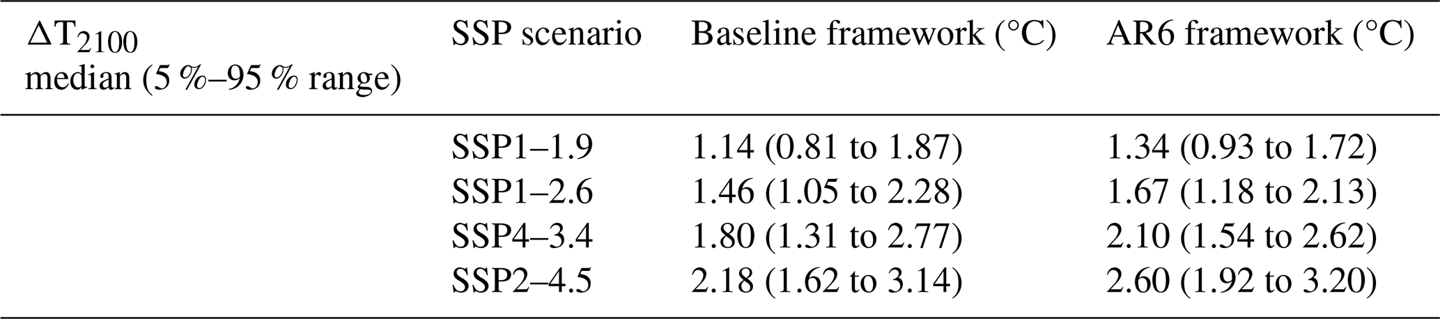
Figures S4 and S5 in the Supplement show the GMST anomaly in year 2100 (ΔT₂₁₀₀) as a function of climate feedback and ERF_AER, in a manner similar to Fig. 1, for the Baseline and AR6 frameworks, respectively. Probabilistic projections of ΔT₂₁₀₀ are obtained using the same weighting technique that was used for AAWR and EffCS, as described in Sect. 2.2.2. Table 2 provides median as well as 5th and 95th percentile values of ΔT₂₁₀₀ for the four SSP scenarios considered throughout. Median projections of ΔT₂₁₀₀ within the AR6 framework are about 0.2 °C (SSP1–1.9, SSP1–2.6), 0.3 °C (SSP4-3.4), and 0.4 °C (SSP2–4.5) greater than found using the Baseline framework. This difference originates from the fact that projected ERF at the end of the century is higher in the AR6 framework than in Baseline for all four SSPs, which is driven by higher end-of-century atmospheric concentrations of CO₂ and CH₄ in AR6 (Fig. S1i).

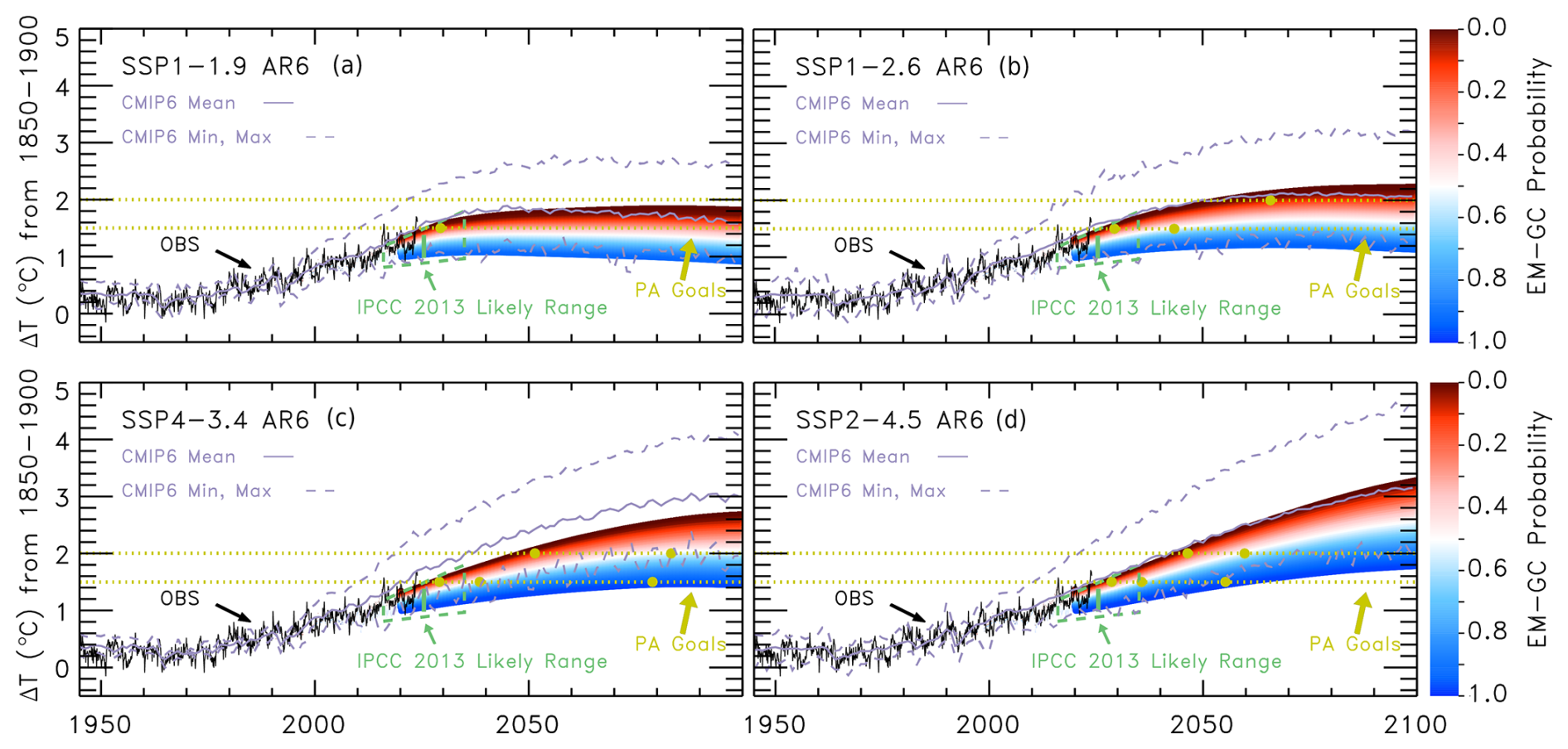
Figure 3 Time-dependent probabilistic forecasts of the GMST anomaly within the AR6 framework. The black line shows the HadCRUT5 GMST anomaly, which was used (along with OHC) to constrain the simulations. Colors represent the probability of reaching a certain temperature or higher at a given time, as indicated by the color bars on the right. The green trapezoid represents the likely range of warming as shown in Fig. 11.25b of the IPCC AR5 report (Kirtman et al., 2013). The target and upper limit of the Paris Agreement are shown by gold-colored horizontal dotted lines. Circle markers on these lines correspond to the projected GMST anomaly crossing these thresholds, with the probability indicated by the colors. The grey lines denote the multi-model mean (solid), as well as the minimum and maximum (dashed) projections of ΔT from CMIP6 ESMs as described in Sect. 3.3.1 of McBride et al. (2021). All values of ΔT shown in this figure are with respect to an 1850–1900 pre-industrial baseline. (a) GMST projections for SSP1–1.9. (b) GMST projections for SSP1–2.6. (c) GMST projections for SSP4–3.4. (d) GMST projections for SSP2–4.5. Results for the Baseline framework are shown in the same fashion in Fig. S6.

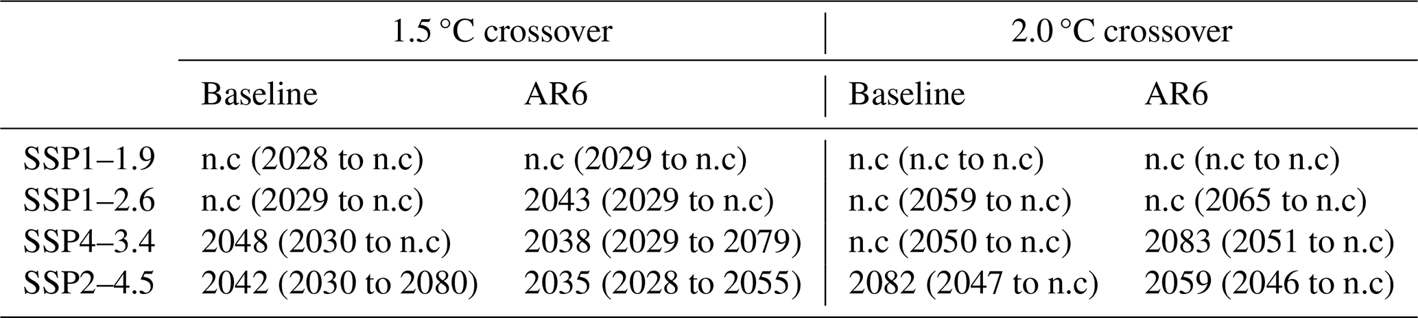
Table 3 Years of crossing the 1.5 and 2.0 °C GMST anomaly thresholds for the four SSP scenarios studied. For each entry, we present the 50 % probability as the central estimate, as well as the 5 %–95 % range. The label “n.c” is used in a manner similar to Table 4.5 of AR6 (Lee et al., 2021) and corresponds to a given threshold not being crossed in the 2020–2100 period.

Next, we examine the temporal evolution of ΔT under the four SSP scenarios. Figure 3 shows time-dependent, probabilistic forecasts of ΔT for the AR6 framework. Time-dependent projections of ΔT for the Baseline framework are shown in Fig. S6 in the Supplement. The colors in Fig. 3 correspond to the probability that ΔT would be equal to or greater than the given numerical value, as indicated by the color bar. Each panel of Fig. 3 also shows the multi-model mean (solid line), and minimum and maximum (dashed lines) for ΔT obtained from the CMIP6 ESM archive, normalized to zero over 1850 to 1900. These CMIP6 values of ΔT are based on the analysis of output from 10, 34, 6, and 32 models for SSP1–1.9, SSP1–2.6, SSP4–3.4, and SSP2–4.5, as described in Sect. 3.3.1 of McBride et al. (2021). Figure 3 also shows the HadCRUT5 GMST observations in black, as well as a green trapezoid that represents the likely range of warming between 2016 and 2035 provided by Chap. 11 of the AR5 report (Kirtman et al., 2013). This trapezoid was placed in Fig. 11.25b of AR5 due to the recognition, by the chapter authors, that the CMIP5 models central to AR5 tended to overestimate the observed rate of global warming. Gold horizontal lines in Fig. 3 represent the 1.5 and 2.0 °C GMST anomalies relative to pre-industrial, while gold circles correspond to the years where the 1.5 and 2 °C thresholds are crossed with 5 %, 50 %, and 95 % probabilities (hereafter termed crossover years). Table 3 provides the years in which the temperature anomaly thresholds are projected to be crossed for the median as well as the 5th and 95th percentiles.

Our probabilistic projections of ΔT are in excellent agreement with the assessed likely range of global warming provided by Chap. 11 of AR5 (Kirtman et al., 2013). Our projections of ΔT fall within the bottom half of those obtained from the CMIP6 ESMs. Numerous studies have similarly concluded that many of the ESMs central to CMIP6 tend to provide estimates of the rate of global warming due to human activity (that is, AAWR) that exceeds empirically based estimates of AAWR (Tokarska et al., 2020b; Nijsse et al., 2020; McBride et al., 2021; Chylek et al., 2024), which Hausfather et al. (2022) have termed the “hot model problem”. Armour et al. (2024) suggested that the high estimates of AAWR exhibited by some of the CMIP6 historical simulations are due to the inability of these models to reproduce observed SST patterns, particularly an observed cooling of the eastern tropical Pacific and a warming of the western Pacific that affects the distribution of clouds in the tropics. Weaver et al. (2024) reached the same conclusion based on an analysis of top-of-the-atmosphere albedo of clouds and aerosols, from radiances observed by NASA and NOAA satellite instruments.

For all four SSP scenarios, the 1.5 and 2.0 °C thresholds are projected to be crossed much earlier based on the simulations of the AR6 framework, relative to those of the Baseline. For example, for SSP2–4.5, the 2.0 °C threshold is projected to be crossed in the years 2059 and 2082 within the AR6 and Baseline frameworks, respectively. The AR6 updates to the ERF from GHGs and aerosols result in nearly a quarter of a century shift forward in crossover year. This finding is consistent with the increases in end-of-century warming (ΔT₂₁₀₀) obtained from the simulations using the AR6 framework, relative to those of Baseline (Table 2). Compared to the literature, the crossover years found here using the AR6 framework fall on the latter end of the projected crossover years for the 1.5 and 2.0 °C thresholds given in Table 4.5 of AR6 (Lee et al., 2021), and are much later than projected based on the analysis of CMIP5 and CMIP6 output shown in Table 1 of Tebaldi et al. (2021). The values in their table are based on an analysis of an unconstrained ESM ensemble, which projects higher levels of future warming than observationally constrained models, as evidenced by Table A6 of Tebaldi et al. (2021).

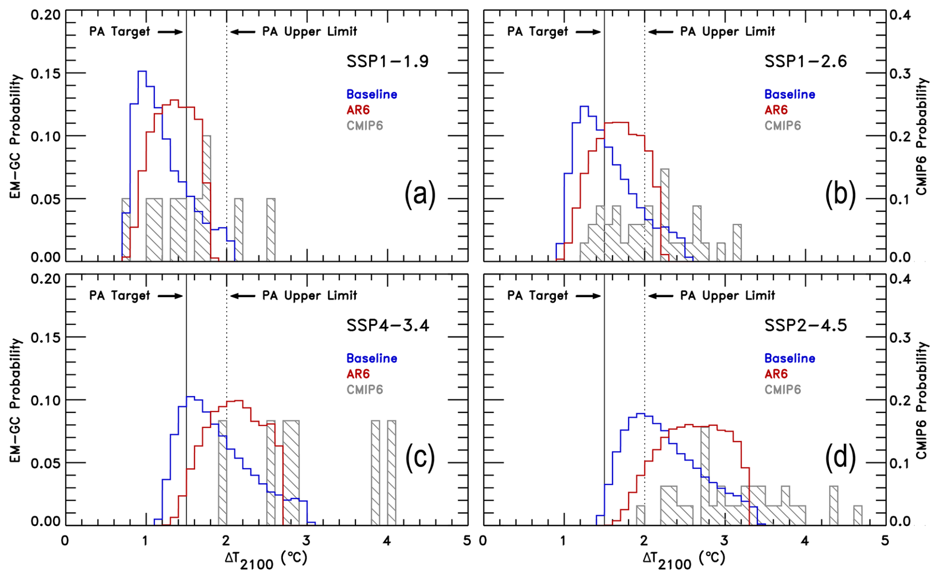
Figure 4 Probability distribution functions (PDFs) for ΔT₂₁₀₀ obtained from EM–GC simulations trained on the HadCRUT5 temperature dataset. Model runs for the Baseline and AR6 frameworks are shown in blue and red, respectively. Grey color represents the PDFs obtained from a CMIP6 multi-model ensemble as described in Sect. 3.3.1 of McBride et al. (2021), and are shown for comparison with EM–GC results. The left-hand y axis corresponds to the EM–GC probabilities, and the right-hand y axis is for the CMIP6 probabilities. The PA target and upper limit are shown as solid and dashed vertical lines, respectively. (a) PDFs for SSP1–1.9. (b) PDFs for SSP1–2.6. (c) PDFs for SSP4–3.4. (d) PDFs for SSP2–4.5.

Figure 4 shows the PDF of ΔT₂₁₀₀ found with EM–GC for the four SSP scenarios, using the AR6 and Baseline frameworks. The height of the bars corresponds to the probability of ΔT₂₁₀₀ being in the range defined by the width of each column. Figure 4 also shows PDFs derived from a CMIP6 ESM ensemble, as detailed by McBride et al., (2021). As expected, based on the “hot model problem” described above, our projections of ΔT₂₁₀₀ within both the Baseline and AR6 frameworks fall on the lower end of the projections from the CMIP6 ensemble. Furthermore, the EM–GC-based PDF for the AR6 framework tends to be shifted towards higher values of ΔT₂₁₀₀ than found for Baseline, with a smaller tail, behaviors that are consistent with higher end-of-century RF of the climate within the AR6 framework (Fig. S1i), as well as the ability to fit the climate record with higher values of climate feedback (model parameter λ_Σ) in the Baseline framework (Fig. 1).

We now further compare our projections of ΔT₂₁₀₀ from the AR6 framework with results based on CMIP6 model output. Tokarska et al. (2020b) reported that observationally constrained CMIP6 projections of end-of-century warming are 9 % to 13 % lower than unconstrained CMIP6 projections for SSP1–2.6 and SSP2–4.5, respectively. Tokarska et al. (2020b) found the median and 5 %–95 % ranges of end-of-century warming relative to a 1995–2014 baseline to be 0.94 (0.41 to 1.46) °C and 1.84 (1.15 to 2.52) °C for SSP1–2.6 and SSP2–4.5, respectively, using observationally constrained CMIP6 models. The values of ΔT₂₁₀₀ in Table 2, relative to 1995–2014, are 0.81 (0.32 to 1.27) °C and 1.74 (1.06 to 2.34) °C for SSP1–2.6 and SSP2–4.5. Consequently, our quantification of ΔT₂₁₀₀ is in very good agreement with the empirically constrained CMIP6 projections of Tokarska et al. (2020b). Chylek et al. (2024) recently found end-of-century warming to be 2.41 °C relative to pre-industrial conditions for SSP2–4.5 using a set of CMIP6 models that accurately reproduce the 2014–2023 warming, which is about 0.5 °C smaller than the value of ΔT₂₁₀₀ obtained from their unconstrained CMIP6 ensemble. Consequently, their empirically constrained value of ΔT₂₁₀₀ is in good agreement with our median estimate of 2.6 °C for SSP2-4.5 (Table 2).

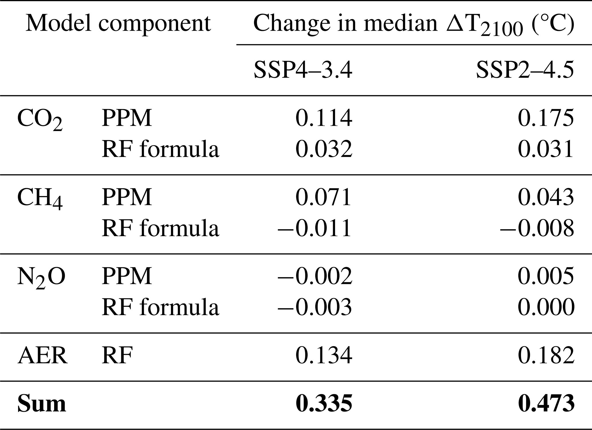
Larger values of ΔT₂₁₀₀ are found in the AR6 framework compared to the Baseline (Table 2). As detailed in Table 4, the more aggressive warming within the AR6 framework is due mainly to three factors: (1) stronger cooling over the historical time period by tropospheric aerosols in the AR6 framework relative to Baseline (Fig. S1e); (2) larger future concentrations of CO₂ projected by AR6 compared to the SSP database (Fig. S1a); (3) greater ERF due to CO₂ using AR6 formula compared to the AR5 formula. Table 4 shows the change in the median value of ΔT₂₁₀₀, found for a series of full ensemble model simulations conducted using the AR6 framework, except for replacement of individual model inputs from the Baseline run. The entry labeled “CO₂ PPM” for SSP4–3.4 represents the difference between a computation of ΔT₂₁₀₀ found using AR6-based model inputs (2.10 °C for SSP4–3.4, as shown in Table 2) and a new median value of ΔT₂₁₀₀ found from a simulation that uses the Baseline projection of the atmospheric concentration of CO₂ (dotted line, Fig. S1a) and AR6 values for all other model inputs (in this case, yielding a median value for ΔT₂₁₀₀ of 1.986 °C for SSP4–3.4). Similarly, the entry labeled “CO₂ RF Formula” shows the difference in ΔT₂₁₀₀ from the full AR6 simulation compared to a run that uses the ERF formula for CO₂ from Table 8.SM.1 of AR5. The fact that the single, largest impact on ΔT₂₁₀₀ is driven by changes to the ERF of tropospheric aerosols, for both the SSP4–3.4 and SSP2–4.5 scenarios, underscores the importance of reducing the current uncertainty in this quantity, to better constrain future projections of global warming. Furthermore, the most important GHG-related factors affecting our forecasts of ΔT₂₁₀₀ are the projections of the future atmospheric concentrations of CO₂ and CH₄, which are notably different within Annex III of AR6 compared to the SSP database. Finally, changes to other inputs between the AR6 and Baseline computations, that are not considered in Table 4 such as the ERF due to tropospheric ozone, halocarbons, and LUC, make small contributions to the differences in the model projections of ΔT₂₁₀₀.

Table 4 Differences between projected median ΔT₂₁₀₀ from the AR6 framework, and model runs where a single model component was replaced with input from the Baseline framework (see the text). The sum of the individual changes is shown in bold in the last row.

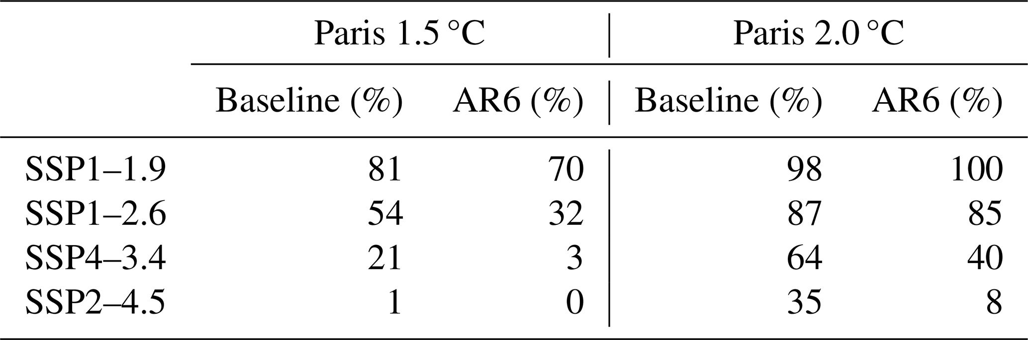
We conclude by evaluating the probability of achieving both the target (1.5 °C) and upper limit (2.0 °C) of the PA. Table 5 provides the probability that end-of-century warming will be below either the target or the upper limit of the PA, relative to pre-industrial conditions. These estimates were obtained from our probabilistic forecasts of ΔT for both the Baseline and AR6 frameworks (Fig. 4). As shown in Table 2, median projections of ΔT₂₁₀₀ are larger within the AR6 framework relative to the Baseline for all four SSPs, which leads to a decline in the probability of accomplishing the PA within the AR6 framework (Table 5). For the SSP1–1.9 and SSP1–2.6 scenarios, the probability of limiting global warming to 2.0 °C is high (at least 85 %) for both model frameworks. For SSP4–3.4, the probability of limiting warming to 2.0 °C falls from 64 % (Baseline) to 40 % (AR6). Most notably, the 2.0 °C probability drops from 35 % to 8 % for the SSP2–4.5 scenario. The 1.5 °C warming probabilities for the AR6 framework are all uniformly lower than found for the Baseline framework, with the SSP1–2.6 scenario dropping from 54 % (Baseline) to 32 % (AR6). The takeaway message from Table 5 is that, for society to have high confidence in achieving at least the upper limit of the PA, the radiative forcing of climate due to GHGs must be placed close to the SSP1–2.6 pathway over the coming decades. More aggressive reductions in GHG radiative forcing are needed to achieve the target of the PA, such as those of the SSP1–1.9 scenario. This message stands in stark contrast to the prior statement in McBride et al. (2021), that SSP4–3.4 would provide about a two-thirds chance of limiting global warming to 2 °C by the end of the century, since this earlier work relied upon the Baseline framework.

Table 5 EM–GC-computed probabilities of achieving the Paris Agreement target (1.5 °C) and upper limit (2.0 °C). Columns with the “Baseline” header represent EM–GC simulations using the Baseline framework, while “AR6” represents simulations of the AR6 framework. The values presented in this table are derived from the PDFs shown in Fig. 4.

4 Conclusions

The extent of global warming is proportional to the ERF from greenhouse gases and tropospheric aerosols. In this work, we use a multiple linear regression energy balance model (EM–GC) to quantify how updates to the projections of effective radiative forcing (ERF) due to GHGs and tropospheric aerosols given by the IPCC AR6 report impact estimates of attributable anthropogenic warming, climate sensitivity, and projected future increases in GMST. We focus on four policy-relevant SSP scenarios: SSP1–1.9, SSP1–2.6, SSP4–3.4 and SSP2–4.5 (O'Neill et al., 2014, 2016).

We show that projected total anthropogenic ERF (ERF_ANTH) computed from AR6 forecasts of the atmospheric concentrations of GHGs, AR6 changes to the parameterizations of ERF due to GHGs, and AR6 updates to the radiative effects of tropospheric aerosols (termed the AR6 framework) results in considerably larger values of projected ERF_ANTH compared to values in the Baseline framework, which represents the state of knowledge prior to AR6. It is important to note that ERF_ANTH found in both the AR6 and Baseline frameworks relies on the same emission time series for GHGs. The higher values of ERF_ANTH in the AR6 framework relative to Baseline is driven by updates to future atmospheric concentrations of CO₂ and CH₄ due to the use by AR6 of a new version of the Model for the Assessment of Greenhouse Gas Induced Climate Change (MAGICC) model (Meinshausen et al., 2011a, b, 2020), updates to the mathematical formulations of ERF due to GHGs in AR6 that results in about a 6 % increase in the radiative forcing of climate for “doubled CO₂” relative to the AR5 parameterization (Forster et al., 2021), as well as major changes in the assessed values of the magnitude and temporal evolution of ERF due to tropospheric aerosols by AR6. The combination of these factors results in about a 0.9 W m⁻² increase in the end-of-century value of ERF_ANTH for the SSP2–4.5 scenario for AR6 compared to Baseline. While some minor deviation of end-of-century ERF_ANTH from the nameplate RF value of SSP scenarios is expected (that is, 4.5 W m⁻² radiative forcing for SSP2–4.5) (van Vuuren et al., 2014), the AR6 updates increase ERF_ANTH such that end-of-century values are now considerably larger than the nameplate RF for each of the four SSP scenarios we have examined.

The rate of human-induced warming between 1974 and 2014 (AAWR) was found to be 0.18 (0.13 to 0.21) °C per decade within the AR6 framework, a slight increase relative to the central estimate and range of 0.16 (0.12 to 0.20) °C per decade for the Baseline framework (the range reflects the 5th and 95th percentiles). Our estimate of AAWR within the AR6 framework was shown to be consistent with other recent studies that adopt various means to separate human and natural influence on GMST (Gulev et al., 2021; Forster et al., 2023; Samset et al., 2023). Most importantly, our estimate of AAWR is lower than values found by many of the free-running (that is, unconstrained by observed GMST) CMIP6 ESMs (Tokarska et al., 2020b; McBride et al., 2021; Tebaldi et al., 2021; Hausfather et al., 2022; Chylek et al., 2024)

The magnitude of EffCS inferred from the historical GMST record was found to be 2.29 (1.54 to 3.11) °C within the AR6 framework and 2.26 (1.45 to 4.37) °C for the Baseline framework. Although the median value of EffCS is nearly identical between the two frameworks, there is a narrower range within the AR6 framework. The narrower range is driven by the ability to obtain good fits to the historical GMST record for a larger values of climate feedback within the Baseline framework compared to AR6, which we have shown is driven by large differences in the assessed temporal evolution of cooling by tropospheric aerosols in AR6 compared to Baseline. Using the AR6 best estimate for the pattern effect (α^′ in Eq. 2) of 0.5 $\mathrm{W}{\mathrm{m}}^{-\mathrm{2}}\mathrm{°}{\mathrm{C}}^{-\mathrm{1}}$ (Forster et al., 2021), we find values for ECS of 3.24 (1.92 to 5.15) °C for the AR6 framework. This estimate of ECS is quite similar to the AR6 assessment of 3.0 (2.0 to 5.0) °C given in Table 7.13 of Forster et al. (2021). Overall, the estimates of EffCS and ECS found within the AR6 framework compare quite well with values reported by several other recent analyses of the climate system (Rugenstein et al., 2020; Skeie et al., 2024; Armour et al., 2024).

The computational efficiency of the EM–GC allows for probabilistic projections on future warming that rely on consideration of the uncertainty in the magnitude of ERF from tropospheric aerosols as well as climate feedback. Median projections on end-of-century warming (ΔT₂₁₀₀) found using our model are higher, by 0.2 to 0.4 °C, for the AR6 framework relative to projections found in the Baseline framework. Both frameworks rely upon the same time series for the future emissions of GHGs. The larger projected warming within the AR6 framework is driven by AR6 updates to projections of the atmospheric concentrations of GHGs, the ERF of GHGs, and the temporal evolution of aerosol cooling.

Finally, we evaluate the likelihood of achieving either the target (1.5 °C) or upper limit (2 °C) warming thresholds of the PA. The AR6 updates to GHGs and aerosols result in a decline in the likelihood of limiting warming to either 1.5 or 2 °C, compared to Baseline. Below, we give numerical results for only the AR6 framework. Model simulations using SSP2–4.5 (designed to reflect trends in the absence of further climate policies) and SSP1–2.6 (full implementation of currently proposed emission targets; Meinshausen et al., 2024), are found to offer no chance and a 32 % chance of limiting the rise in GMST to 1.5 °C by 2100. Model simulations conducted using SSP4–3.4 (intermediate scenario between SSP1–2.6 and SSP2–4.5) and SSP1–1.9 (aggressive future reductions in GHG emissions) show probabilities of 3 % and 70 % of limiting warming to 1.5 °C by the end of the century. The likelihood of limiting warming to 2.0 °C is found to be 8 %, 40 %, 85 %, and 100 % for the SSP2–4.5, SSP4–3.4, SSP1–2.6, and SSP1–1.9 scenarios, respectively.

In earlier work using the EM–GC that relied upon the Baseline framework, McBride et al. (2021) concluded that the SSP4–3.4 scenario provided a 64 % probability of limiting global warming to 2 °C by the end of the century. The AR6-based updates to ERF_ANTH considered here result in a lower, 40 % probability of achieving this upper limit of the PA. Nonetheless, the EM–GC-based estimates of limiting end-of-century warming to 2 °C for both the AR6 and Baseline frameworks are more optimistic than is provided by many free-running CMIP6 ESMs. Our results suggest that SSP1–2.6 is the “two-degree pathway”, since this scenario provides an 85 % probability of limiting global warming to the upper limit of the PA.