Earth's future climate and its variability simulated at 9 km global resolution

Earth's climate response to increasing greenhouse gas emissions occurs on a variety of spatial scales. To assess climate risks on regional scales and implement adaptation measures, policymakers and stakeholders often require climate change information on scales that are considerably smaller than the typical resolution of global climate models (O(100 km)). To close this important knowledge gap and consider the impact of small-scale processes on the global scale, we adopted a novel iterative global earth system modeling protocol. This protocol provides key information on earth's future climate and its variability on storm-resolving scales (less than 10 km). To this end we used the coupled earth system model OpenIFS–FESOM2 (AWI-CM3; Open Integrated Forecasting System – Finite volumE Sea ice–Ocean Model) with a 9 km atmospheric resolution (TCo1279) and a 4–25 km ocean resolution. We conducted a 20-year 1950 control simulation and four 10-year-long coupled transient simulations for the 2000s, 2030s, 2060s, and 2090s. These simulations were initialized from the trajectory of a coarser 31 km (TCo319) SSP5-8.5 transient greenhouse warming simulation of the coupled model with the same high-resolution ocean. Similar to the coarser-resolution TCo319 transient simulation, the high-resolution TCo1279 simulation with the SSP5-8.5 scenario exhibits a strong warming response relative to present-day conditions, reaching up to 6.5 °C by the end of the century at CO₂ levels of about 1100 ppm. The TCo1279 high-resolution simulations show a substantial increase in regional information and climate change granularity relative to the TCo319 experiment (or any other lower-resolution model), especially over topographically complex terrain. Examples of enhanced regional information include projected changes in temperature, rainfall, winds, extreme events, tropical cyclones, and the hydroclimate teleconnection patterns of the El Niño–Southern Oscillation and the North Atlantic Oscillation on scales of less than 1000 km. The novel iterative modeling protocol that facilitates coupled storm-resolving global climate simulations for future climate time slices offers major benefits over regional climate models. However, it also has some drawbacks, such as initialization shocks and resolution-dependent biases and climate sensitivities, which are further discussed.

1 Introduction

Previous generations of global climate models have revealed fundamental insights into the large-scale response of the climate system to past and future anthropogenic greenhouse forcing. To further provide crucial information on regional scales, several international and domestic regional downscaling efforts have been launched, such as the Coordinated Regional Climate Downscaling Experiment (CORDEX) (Fig. 1), which – depending on the domain of interest – simulates climate features down to scales of 8–25 km (Giorgi et al., 2012; Jacob et al., 2014; Giorgi and Gutowski, 2015; Gutowski et al., 2016). This scale is of crucial interest to stakeholders who plan to assess risks of future climate change or implement specific climate change adaptation measures (Lesnikowski et al., 2016; Pacchetti et al., 2021; Biswas and Rahman, 2023; Petzold et al., 2023; Jebeile, 2024). One of the disadvantages of regional model projections is that they use boundary condition input fields of coarser-resolution global models, which often do not properly resolve important mesoscale processes, such as tropical cyclones. Another modeling approach that was pursued previously is pseudo-global-warming experiments, in which coarser-resolution Coupled Model Intercomparison Project (CMIP)-based sea surface temperature (SST) patterns were used to force high-resolution atmospheric models with resolutions down to 8 km or less (Jung et al., 2012; Kinter et al., 2013). As of recently, however, running global fully coupled earth system models on scales of regional models has been prohibitively expensive and beyond the capability of many supercomputers. Only in the last 2 years have examples of seasonal (Hohenegger et al., 2023) and multi-year (Rackow et al., 2025) simulations of coupled kilometer-scale climate models been made available.

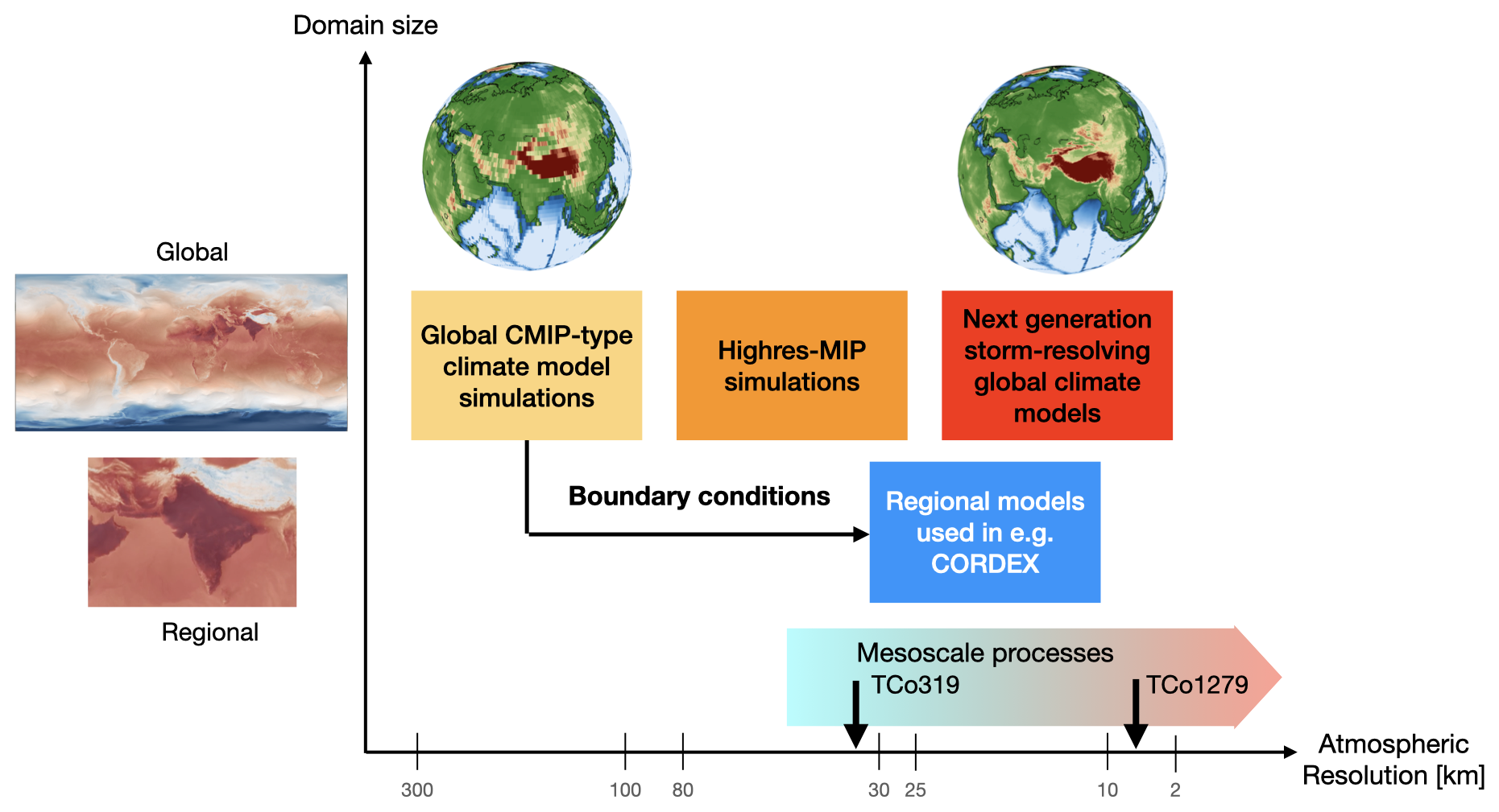
Figure 1 Schematics illustrating the modeling hierarchy of global and regional earth system models used for future climate change projections. The global and regional equirectangular projection maps are snapshots of 2 m air temperature from the AWI-CM3 TCo1279 model. The two upper globular maps depict topography from TCo95 (100 km, left) and TCo1279 (9 km, right). Model simulations in this study are based on the OpenIFS–FESOM2 (AWI-CM3) model, which uses TCo319 and TCo1279 (cubic-octahedral spectral truncation) at 31 and 9 km, respectively. Our TCo1279 global model simulation employs a horizontal resolution that is similar to that used in regional models, such as in CORDEX simulations. The atmosphere and ocean model setups and resolutions for the TCo319 and TCo1279 configurations of the AWI-CM3 model are depicted in Figs. 2 and 3.

One of the first coordinated efforts to conduct coupled greenhouse warming simulations until 2050 CE with resolutions higher than the ones used in global earth system models, which participated in CMIP Phase 6 (Eyring et al., 2016; Danabasoglu et al., 2020; Meehl et al., 2020), is the HighResMIP modeling project (Haarsma et al., 2016) (Fig. 1). In HighResMIP and other related global coupled modeling efforts (Chang et al., 2020; Huang et al., 2021b), earth system models adopted atmospheric resolutions of about 25 km or larger. This higher-resolution perspective on climate change has revised substantially our understanding of key climate processes and their sensitivity to various types of forcings, including the El Niño–Southern Oscillation (Wengel et al., 2021), tropical cyclones (Vecchi et al., 2019; Chu et al., 2020; Raavi et al., 2023), the East Asian Summer Monsoon (Liu et al., 2023), or atmospheric rivers (Nellikkattil et al., 2023). Still climate models that run at this resolution or finer (Hohenegger et al., 2023; Rackow et al., 2025) require extensive computing resources, which limits the number and length of model simulations that can be conducted, including even test simulations, spin-ups, or optimization runs that need to be performed to obtain a realistic modern climate mean state.

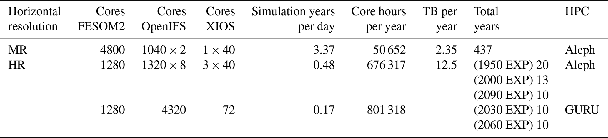
To close the resolution gap between regional climate models that only cover specific geographic domains and global climate models, it is necessary to use modeling systems that are highly scalable on high-performance computing (HPC) systems and that can be readily configured in different resolutions. To this end, we chose to conduct greenhouse warming simulations with the OpenIFS–FESOM2 (AWI-CM3; Open Integrated Forecasting System – Finite volumE Sea ice–Ocean Model) model (Fig. 2), which has been adopted in recent studies for atmospheric resolutions of 100, 61, and 31 km (Streffing et al., 2022; Shi et al., 2023). The AWI-CM3 model uses the ECMWF IFS TCo atmospheric grids. For this grid type the theoretically infinite spectral space is truncated to truncation number T, and in grid point space a cubic octahedral (Barker et al., 2020) reduced Gaussian grid with four grid points sampling the smallest spherical harmonic is used (Malardel et al., 2015). The IFS numerical implementation of the hydrostatic dynamical core scales extremely well on HPC systems (Table 1) and serves as one of the principal enablers of the work we present here using the AWI-CM3 fully coupled model.

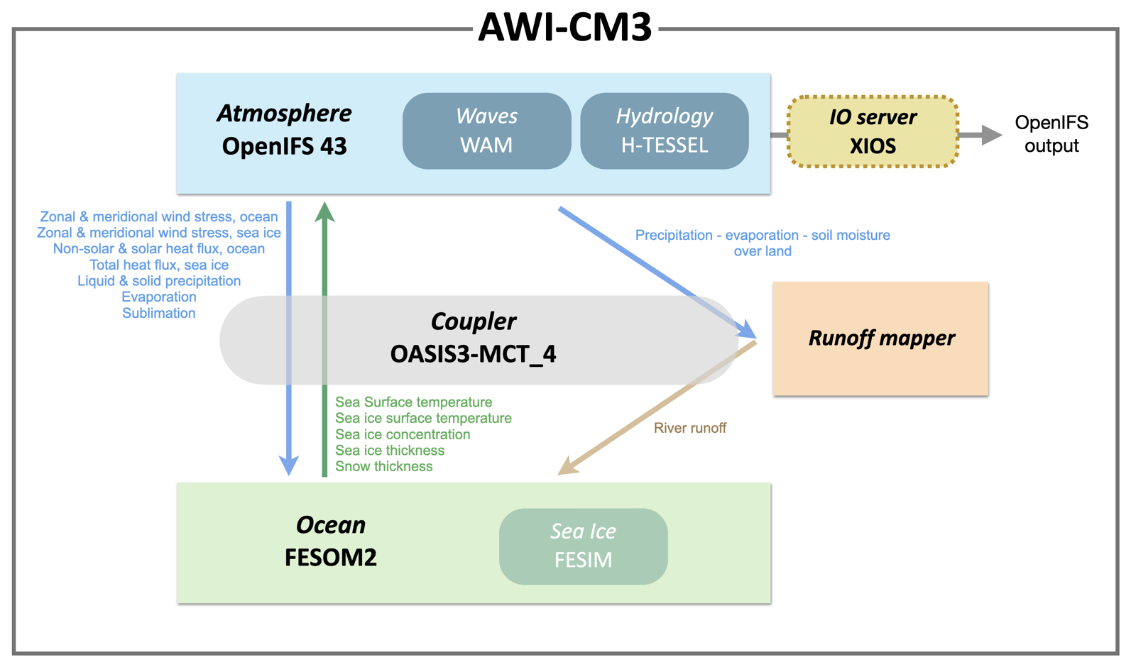
Figure 2 Schematics of Alfred Wegener Institute Climate Model version 3 showing the modeling subcomponents used for the MR and HR setups. Subcomponents including atmosphere, ocean, and runoff mapper exchange their states and fluxes via an OASIS coupler. XIOS is an I/O server that can be run parallel to OpenIFS and manages output from the OpenIFS model. Updated from Fig. 1 in Streffing et al. (2022). See Sect. 2 for details on the individual model components.

The primary goals of our study are (1) to identify the fidelity of the high-resolution model and its biases under present-day conditions; (2) to simulate future climate change with a state-of-the art coupled earth system model at atmospheric scales of 9 km and comparable ocean scales; (3) to provide key information on the regional aspects of mean changes in temperature, precipitation, and wind; and (4) to further document shifts in extreme events and modes of climate variability, such as the Madden–Julian oscillation (MJO), the El Niño–Southern Oscillation (ENSO), and the North Atlantic Oscillation (NAO). This is achieved by first conducting a transient simulation with the SSP5-8.5 greenhouse gas concentration scenario at lower atmosphere resolution (31 km, TCo319) but with the same ocean resolution and branching off 13-year- and 10-year-long coupled simulations with the higher atmosphere resolution (9 km, TCo1279) for the 2000s, 2030s, 2060s, and 2090s (Fig. 4). In addition, a 20-year-long control simulation is conducted at high resolution which uses constant 1950 greenhouse gas and aerosol conditions. We also repeated the 2090s chunk on the Korea Meteorological Administration (KMA) supercomputer GURU. The results from this additional experiment are only used in Sect. 6 to extend the dataset that is used for the analysis of changes in extreme events, climate variability, and teleconnections. To the best of our knowledge, these new simulations are the highest-resolution fully coupled global simulations of future climate change reaching 2100 CE conducted to date.

The paper is organized as follows: in Sect. 2 we will introduce the AWI-CM3 model setup and its performance for the TCo319 and TCo1279 resolutions. Section 3 provides an overview of the high-resolution present climate simulations in terms of both atmospheric and oceanic processes. Section 4 describes the sensitivity of the model to future climate change and presents global-mean-temperature-normalized climate change patterns, and Sect. 5 focuses on the present and future statistics of atmospheric extreme events. Our paper further emphasizes the impact of modes of natural climate variability on regional climates and how these impact/teleconnection patterns may change in the future (Sect. 6). Section 7 concludes with a summary and discussion.

While this paper features new scientific results on the high-resolution response of the earth climate system to greenhouse warming, it also proposes a novel protocol for high-resolution coupled simulations and provides a reference for the TCo1279 AWI-CM3 simulations. The data access links are shared in the corresponding section.

2 Model description and experimental setup

Our study is based on the AWI-CM3 coupled climate model (Streffing et al., 2022), which employs the OpenIFS (Open Integrated Forecasting System) atmosphere (cycle 43r3) (Huijnen et al., 2022; Bouvier et al., 2024; Savita et al., 2024) with hydrostatic approximation, the WAM (Wave Model) surface gravity wave model (Komen et al., 1996), and the hydrology model H-TESSEL (Hydrology in the Tiled ECMWF Scheme for Surface Exchanges over Land) (Balsamo et al., 2009) (Fig. 2). The ocean model used is the Finite volumE Sea ice–Ocean Model (FESOM2) (Danilov et al., 2017; Koldunov et al., 2019a; Scholz et al., 2019), which also includes the FESIM (Finite-Element Sea Ice Model) sea-ice module (Danilov et al., 2015). The model components are communicating with each other via the OASIS3–MCT coupler (Ocean Atmosphere Sea Ice Soil coupler interfaced with Model Coupling Toolkit) (Fig. 2) and the runoff mapper. The OpenIFS output is managed through a parallel XML input/output server (XIOS). For the simulations described in this study, we choose two different model configurations: the first is the “medium-resolution” setup (from here on MR) with a TCo319 atmosphere resolution (Fig. 3a), featuring a grid spacing of about 31 km near the Equator and up to 38 km at high latitudes. The ocean uses the FESOM2 DART mesh, which employs a spatially variable resolution (Fig. 3c) to optimally resolve the regional Rossby radius of deformation in regions with high eddy activity (Streffing et al., 2022). In the Arctic, the ocean grid size corresponds to about 5 km, which can resolve large-scale sea-ice cracks (“Video supplement” S1, S2, Moon et al., 2024b) (Wekerle et al., 2013; Wang et al., 2018; Koldunov et al., 2019b; Moon et al., 2024b). For the tropical ocean, an average resolution of about 12–25 km is adopted, which allows for a reasonable representation of tropical instability waves (Small et al., 2003; Holmes et al., 2019) and island effects (Eden and Timmermann, 2004) (“Video supplement” S3, Moon et al., 2024b). Moreover, the DART mesh exhibits increased spatial resolution of about 7.5–10 km in coastal regions. This improves the representation of nearshore processes, such as upwelling, coastal eddies, or shelf interactions, which are often not properly resolved in lower-resolution climate models.

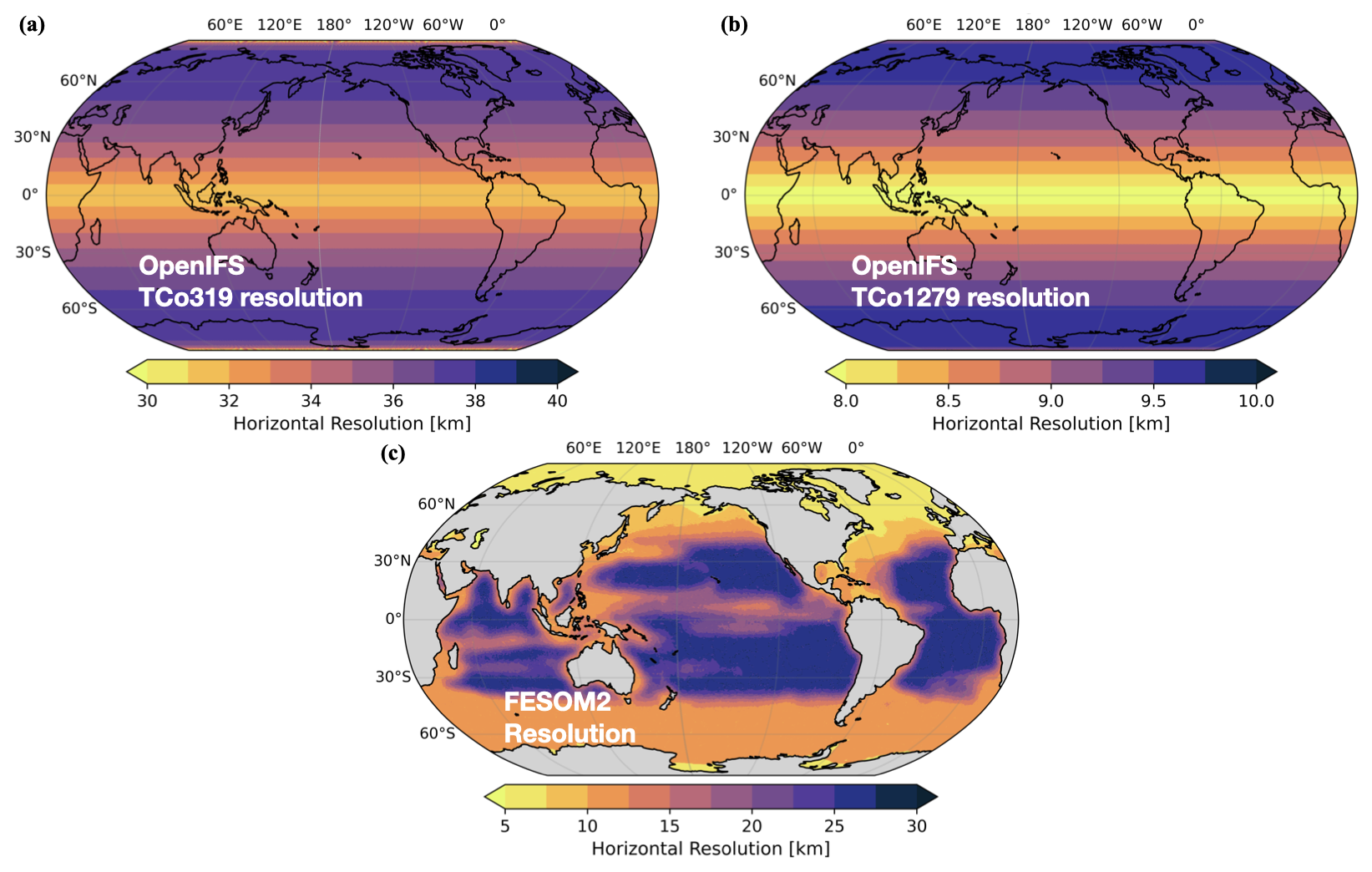
Figure 3 Horizontal resolution of (a) TCo319 medium-resolution (MR) and (b) TCo1279 high-resolution (HR) configurations of the OpenIFS and the (c) FESOM2 DART mesh used for both MR and HR simulations.

In addition to the MR configuration, we also run the AWI-CM3 model with a high-resolution setup (hereafter referred to as HR), where OpenIFS uses a TCo1279 truncation. This configuration attains the highest resolution of about 8 km near the Equator, and the lowest is about 10 km at high latitudes (Fig. 3b, right panel). This is the resolution realm that is normally adopted in regional climate models and current operational weather forecast models (Fig. 1). It is suitable to represent the regional features of tropical cyclones and capture the topographic details of prominent mountain ranges on our planet. The MR and HR configurations both use the same DART 80-layer ocean mesh and 137 pressure levels in the atmosphere extending from the surface to 0.01 hPa in the upper stratosphere. In both configurations, the vertical configuration of the atmospheric model setup is sufficient to capture to some degree important stratospheric phenomena such as sudden stratospheric warming events and the Quasi-Biennial Oscillation.

To perform HR global warming time-slice simulations extending to 2090–2100 CE, we first conducted a 100-year-long MR spin-up simulation using 1950 atmospheric greenhouse gas and aerosol conditions. This run is not further discussed here, but its end state is used as the initial condition for our 184-year-long MR fully coupled control simulation (Fig. 4). The control run exhibits stable global mean surface temperatures of about 14 °C, which compares well with the observational estimates (Hersbach et al., 2023) (Fig. 4) and shows only little radiative imbalance at the top of the atmosphere (i.e., difference between net shortwave radiation and net thermal radiation at the top of atmosphere, both positive downward) of < ±0.5 W m⁻². The 1950 spin-up also serves as the initial condition for a transient MR scenario simulation (1950–2100), which uses historical forcings from 1950 to 2014 CE and greenhouse and aerosol forcing of the emission-intensive SSP5-8.5 greenhouse gas concentration scenario (Meinshausen et al., 2017) subsequently. The simulation reaches a CO₂ level of 1135 ppm by 2100 CE, and the transient global mean temperature attains values of ∼ 20.5 °C, about 6.5 °C above 1950 levels with a top-of-atmosphere radiative imbalance of about 2 W m⁻². The corresponding transient climate response (TCR) is estimated at ∼ 3 °C per CO₂ doubling, which is on the higher end of the likely range (TCR 1.5–3 °C and equilibrium climate sensitivity (ECS) 1.8–5.6 °C) of CMIP6 models (Meehl et al., 2020). It is, however, comparable to that of other higher-end climate sensitivity models, such as E3SM-1-0 (Caldwell et al., 2019; Golaz et al., 2019), which exhibits an ECS of > 5 °C per CO₂ doubling.

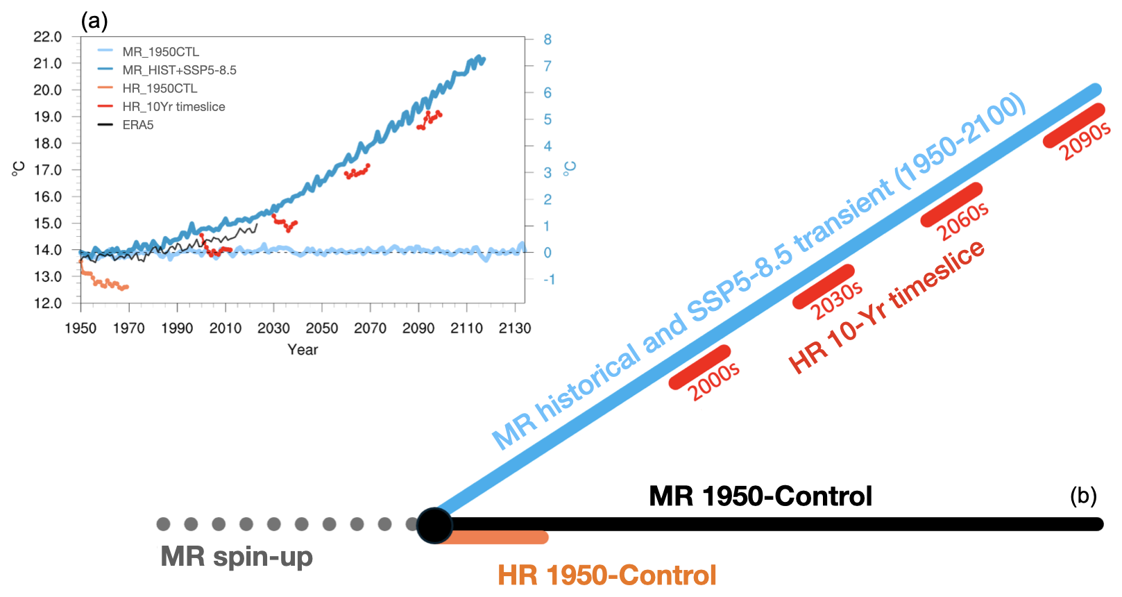
Figure 4 Schematics of setup for transient global warming time-slice simulations along with simulated global mean surface temperatures for experiments listed in Table 1: MR simulation control run (light blue), MR historical and SSP5-8.5 simulation (dark blue), HR 1950 control simulation (orange), and HR SSP5-8.5 transient 10-year time-slice simulation (red). Panel (a) shows the simulated global mean temperatures in the simulations as well as an observational estimate from the ERA5 reanalysis (Hersbach et al., 2023).

The 10-year-long HR time-slice simulations, which are driven by transient SSP5-8.5 forcings, are branched off from the MR SSP5-8.5 run with ocean initial conditions corresponding to 2000, 2030, 2060, and 2090 CE. The atmospheric and land initial conditions for each of these time slices are not taken from the MR simulation (due to technical implementation difficulties) but rather from archived data from ECMWF for the OpenIFS model, version v43r3, which correspond to the year 1990 (https://confluence.ecmwf.int/display/OIFS/6.2+OpenIFS+Input+Files, last access: 16 December 2020). This atmosphere–land “cold start” can potentially cause some initialization shocks. To quantify the robustness of the climate signal from the initialization cold drift (Fig. 4a), we restarted a set of MR simulations at the same time as the HR time-slice simulations using the same 1990 land conditions. A comparison of their respective global mean surface temperature evolution (Fig. S1 in the Supplement) clearly shows that there are no substantial differences between the fully transient MR simulation (in blue) and the new MR time-slice simulations with 1990 land initial conditions (Fig. S1 in purple), indicating that land surface initialization only plays a minor role in causing the observed multi-year drift in Fig. 4a. Furthermore, we analyzed the top-of-atmosphere (TOA) radiation imbalance (Fig. S2) directly after the 1990 land initializations, and we observe a noticeable impact in the HR time-slice simulation only in the first 1–2 years. To minimize the impact of such drifts in our analyses, we remove the first 2 years. The TOA radiative imbalances in our MR and HR control simulations are all in the range of < ±1 W m⁻². Based on the new MR time-slice simulations we conclude that the additional drift occurs because the coupled HR and MR simulations (even with the same ocean setup) have either different climate background states or different climate sensitivities, caused, e.g., by different cloud feedback strengths.

Table 1 Model performance of the OpenIFS–FESOM2 model at MR (TCo319, 31 km) and HR (TCo1279, 9 km) horizontal resolution. EXP signifies experiment.

Apart from the initial drift, we further observe that the HR simulation is in general colder than the MR experiment. This offset is particularly pronounced for the 20-year-long HR 1950 control simulation, which shows longer-term global mean temperature levels ∼ 1.5 °C below the MR control run (Fig. 4a). The HR time-slice simulations are also subject to transient greenhouse gas and aerosol forcings following the SSP5-8.5 protocol and can therefore be considered short transient simulations, which will adjust over time to a transiently forced climate change trajectory.

All major components of AWI-CM3 were developed with scalability as one of the primary design criteria in mind. The base-level MR simulations are performed at around 3.37 simulation years per day (SYPD) on 6920 cores of “Aleph”, the Cray XC50-LC system at the Institute for Basic Science, Daejeon, South Korea. Typically, we ran several MR (TCo319L137_DART) simulations in parallel on Aleph. On the same HPC system the HR (TCo1279L137-DART) model setup with the 9 km atmosphere ran at nearly half a year per day, utilizing 11 960 cores (Table 1). The cost of the HR simulations is about 676 000 core hours per year, compared to around 50 000 core hours per year for the MR simulations. All simulations together (including spin-up simulations) used about 67×10⁶ CPU hours on South Korea's IBS supercomputer Aleph and the GURU supercomputer at the Korea Meteorological Administration (KMA). Faster MR simulations at up to 7.9 SYPD would have been possible at the cost of using the whole Aleph HPC system for one experiment. One of the major challenges of the simulations is the storage and associated analyses of the output data. A total of about 1.8 PB of output data were generated and analyzed. For OpenIFS we employed the XIOS I/O server, allowing the parallelization of data output, with some on-the-fly in-memory processing before data are written to disk for the first time. We also restricted some of the output variables for the HR simulations and used NetCDF data compression to save disk space.

3 Model performance

To assess the fidelity of the MR and HR simulations, we calculate the difference between simulated climatic fields with observational estimates (Figs. 5, S3, S4,). Comparing the simulated sea surface temperatures (SSTs) in the MR and HR historical simulations with an observational climatology (EN4; Good et al., 2013) (Figs. S3, S4, upper right), we find an equatorial Pacific cold bias and a warm bias in the tropical Pacific and Atlantic stratus cloud regions. This bias is qualitatively similar to the ensemble mean bias found in the latest CMIP models (Bock et al., 2020) but with reduced magnitude for the AWI-CM3 simulations compared to many of the individual CMIP models. We also find a notable reduction in the SST biases in the MR and HR historical simulations relative to CMIP models in the western boundary current regions (e.g., Kuroshio Current and its extension and the Gulf Stream). With an ocean resolution of about ∼ O(5–10 km) higher than typical CMIP models in these regions (Fig. 3c), the MR and HR simulations can resolve frontal systems more realistically, as well as mesoscale ocean eddies (Fig. 6, “Video supplement” S3, Moon et al., 2024b), which contribute to heat transport and recirculation. Given that MR and HR use the same ocean model resolution and the fact that the HR 2000 simulation has been run only for 13 years, their respective western boundary current biases are very similar to each other.

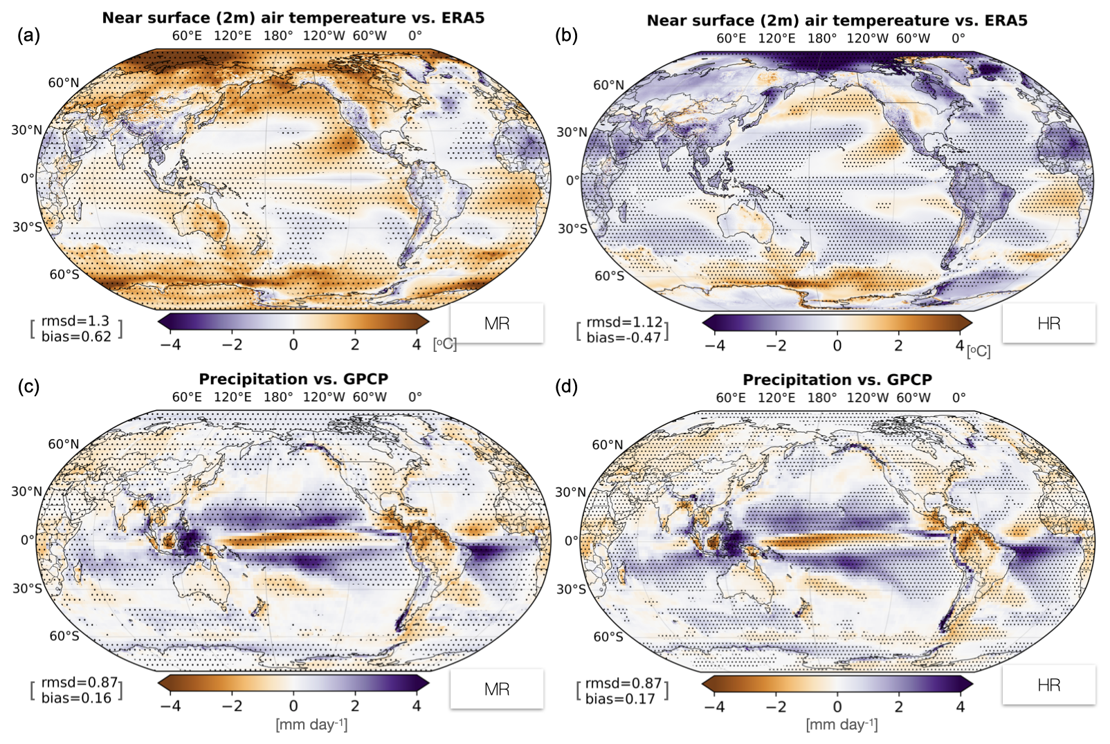
Figure 5 Bias map for MR (a, c) and HR (b, d) historical simulations for long-term mean 2 m air temperature (a, b) and precipitation (c, d) averaged over the years 2002–2012 compared to ERA5 reanalysis and GPCP (Adler et al., 2003; Adler et al., 2012) from 1989–2014. RMSD and bias refer to the root mean squared deviation and the global mean difference between model and reference product. The stippled areas indicate areas where the null hypothesis can be rejected at the 95 % confidence level by Welch's t test. We used the default settings in the stats module SciPy (version 1.11.1) in Python, which applies Welch's t test at every grid point allowing for unequal variances.

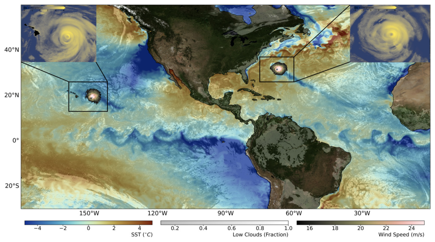
Figure 6 Snapshot (10 September 1969) from HR AWI-CM3 20-year 1950 control model simulation showing 3-hourly data of SST (blue and red shading) minus zonal mean, low clouds (transparent gray and white shading), and 10 m wind speed (green and pink shading). Hurricane precipitation (blue and yellow shaded) is shown in insets. The figure illustrates the ubiquity of mesoscale climate phenomena that can best be simulated at high spatial resolution, such as tropical instability waves in the equatorial Atlantic and Pacific, hurricanes (making landfall in Hawaii in this simulation snapshot), ocean cold wakes generated by hurricanes, stratocumulus cloud decks, and patchy daytime convection over the Amazon forest.

The tropical SST biases (Figs. S3, S4) are in part also imprinted on the 2 m near-surface air temperatures (SAT) (Fig. 5a, b). In addition, we find pronounced SAT biases in polar regions (Fig. 5a) with overestimated temperatures in the Southern Ocean both for MR and HR and opposing signs between MR (warm) and HR (cold) in the Arctic Ocean. Positive biases are evident in both simulations in the midlatitude storm track regions as well as in the subtropical marine stratus cloud regions, which are characterized by negative biases in total cloudiness (Figs. S3a, S4a). Over sea ice and land the surface temperature biases relative to the 1989–2014 period in ERA5 (Hersbach et al., 2023) are most pronounced over the Barents Sea, central United States, the Sahara region, eastern Siberia, and eastern Australia. Averaged globally, the 2002–2012 SAT biases in MR and HR amount to 0.62 and −0.47 °C, respectively. This implies that certain climate states emerge on average earlier in our MR simulation than they would in the real world. In terms of the global mean cloudiness (relative to the MODIS satellite data), the MR simulation exhibits a smaller bias (−0.28 %) for the 2002–2012 period compared to the HR experiment (−2.32 %) (Figs. S3a, S4a). Regional patterns in cloud biases likely contribute to temperature biases and vice versa, particularly in tropical and trade-wind regions. However, disentangling and quantifying the coupling between temperature and cloud biases require a more sophisticated regional feedback analysis (Stowasser and Hamilton, 2006), which is beyond the scope of this paper.

Despite some differences in SAT and SST, including different global mean values, the precipitation bias patterns (relative to the Global Precipitation Climatology Project (GPCP) dataset) for MR and HR are almost identical (Fig. 5c, d). This can be understood by the fact that, at least in the tropical atmosphere, convective precipitation is largely controlled by wind convergence, which emerges in response to SST gradients (Lindzen and Nigam, 1987). Therefore, the SST bias gradient patterns, which are very similar in MR and HR, largely control the corresponding precipitation bias patterns. In the tropics, the precipitation biases of MR and HR are weaker than most CMIP6 models (Table S2 in the Supplement). More specifically, the MR and HR rainfall bias patterns are characterized by a weak double Intertropical Convergence Zone (ITCZ) bias in the eastern tropical Pacific (Lin, 2007; Bellucci et al., 2010; Li and Xie, 2014) and a southward ITCZ bias in the Atlantic region. We also see alternating wet and dry biases over the Maritime Continent which need to be considered when interpreting El Niño teleconnections in this area (Sect. 6). Overall, we conclude that by running a multi-metric analysis of the climate model performance indices (Reichler and Kim, 2008) for the period 2002 to 2012, we find that the biases in the MR and HR experiments are on average 32 % and 35 % smaller than for the average CMIP6 model (Table S2), respectively.

To further illustrate the benefit of running mesoscale-resolving coupled atmosphere–ocean models on a global scale, we show a 1 d snapshot from the HR 1950 control simulation (10 September 1969, Fig. 6). The multi-variable overlay map of SST (blue and red shading), low cloud cover (transparent white and gray shading), hurricane wind speed (green and pink shading), and hurricane precipitation (blue and yellow shaded inlays) shows several key features that require high spatial resolution, including tropical instability waves in the Pacific and Atlantic oceans; cold ocean wakes generated by hurricanes (Chu et al., 2020); patchy stratocumulus cloud streets in the subtropical regions; ocean eddies in the Gulf Stream region, some of which were generated by the strong wind forcing associated with bypassing Pacific and Atlantic hurricanes (see also “Video supplement” S3, Moon et al., 2024b); and diurnal convection in the Amazon rainforest (“Video supplement” S4, Moon et al., 2024b). The latter plays a key role in regional moisture recycling. Moreover, we see that stratus cloud bands align with SST fronts along the tropical instability waves, similarly reported by Small et al. (2003). Furthermore, we observe that the high atmospheric resolution allows even for the generation of double-eye-walled precipitation structures in hurricanes and the generation of strong gravity waves off the Hawaiian islands and other topographic features (upper-left inlay in Fig. 6).

As documented in Fig. 6, the HR simulation with AWI-CM3 resolves individual cloud systems, such as stratocumulus clouds or diurnal grid-scale convective anomalies. This will likely influence the overall performance of clouds and their response to increasing greenhouse gas concentrations. This is further illustrated in Figs. S3a–S4a, which reveal a rather realistic representation of total cloudiness in comparison to the MODIS satellite product (Wielicki et al., 1996; Kato et al., 2018; Trepte et al., 2019), with biases occurring mostly in the equatorial Pacific, in the Arctic Ocean, and over Antarctica. We note, however, that satellite cloud retrieval over Antarctica may also be subject to considerable errors.

Overall, our initial assessment of the AWI-CM3 performance demonstrates that the HR model configuration is a suitable tool to simulate future climate at resolutions which were previously only accessible for regional climate models or SST-forced high-resolution global atmospheric models (Jung et al., 2012; Kinter et al., 2013). The relatively weak SST and precipitation biases (Fig. 5) and the very high scalability and supercomputer throughput (Table 1), as well as the versatility of our iterative modeling protocol (Fig. 4), enable us to conduct coupled simulations of future greenhouse warming for various time periods at unprecedented global resolutions.

4 Sensitivity to future climate change

This section provides an overview of simulated HR present-day conditions and the projected future mean changes for several atmospheric and oceanic variables (Figs. 7–11). Corresponding statistical significance levels (95% confidence for null hypothesis rejection) are calculated using Welch's t test at every grid point allowing for unequal variances. Rather than focusing on the individual time periods 2030–2039, 2060–2069, and 2090–2099 CE, we normalize the responses for the transient 10-year HR simulations (relative to the 2000 present-day conditions) by their respective global mean surface temperature changes of 1.0, 2.97, and 4.99 °C (relative to the 2002–2012 historical simulation), respectively (Fig. 4), and consolidate the three estimates obtained from 24 years of simulation data (last 8 years of each 10-year HR segment excluding 2 years of initial adjustment) by averaging them. This allows for a more robust scenario-independent interpretation of the climate change patterns and an easier comparison with experiments conducted with other climate models.

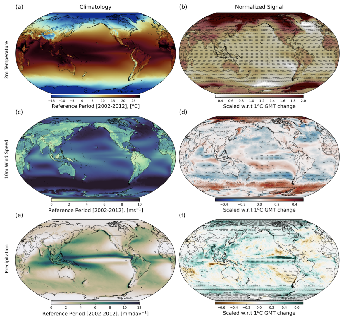
Figure 7 Annual mean climatology of HR simulations during 2002–2012 (a, c, e) and projected climate change signal normalized with respect to a 1 °C global mean temperature (GMT) change (b, d, f) for (a, b) 2 m air temperature, (c, d) 10 m wind speed, and (e, f) precipitation. The stippled areas indicate areas where the null hypothesis can be rejected at the 95 % confidence level using Welch's t test. We used the default settings in the stats module SciPy (version 1.11.1) in Python, which applies Welch's t test at every grid point allowing for unequal variances.

The HR simulations show the typical enhanced polar and land surface warming relative to the global mean (Fig. 7b). Other warming hotspots occur over the Tibetan Plateau, the Hindukush region, northwestern and southern Africa, the Rocky Mountains, the Andes, the Sea of Okhotsk, and the eastern Atlantic subtropical gyre. The future warming pattern is accompanied by large-scale changes in the atmospheric circulation, which are manifested in terms of a weakening of the equatorial Pacific trade winds (along with an enhanced eastern equatorial Pacific warming); a poleward shift and strengthening of the Southern Hemisphere Westerlies, which has been discussed extensively in previous studies (Cai and Cowan, 2007; Biastoch et al., 2009); and an overall intensification of Arctic surface winds (Zapponini and Goessling, 2024) (Fig. 7d). The projected relative precipitation pattern exhibits a massive intensification over the tropical Pacific, which has also been found in CMIP-type greenhouse warming simulations (Collins et al., 2010; Cai et al., 2021; Yun et al., 2021; Ying et al., 2022). However, the HR simulation differs markedly from the lower-resolution CMIP simulations (IPCC, 2014) in that it does not show a strong relative wind speed reduction over the South Pacific subtropical regions. Moreover, in contrast to the CMIP6 multi-model ensemble mean (IPCC, 2023), the HR simulation shows large rainfall anomalies along the southern part of East Asia, in the Philippine Sea, in the East China Sea, and toward the northern part of the North Pacific storm track path.

The representation of small-scale topography also leads to the formation of regional rainfall patterns that cannot be adequately resolved in coarser-resolution coupled general circulation models (Figs. 7e, f and 8). Striking regional features include the rainfall enhancement over the Andes, along the southern flank of the Himalayas, over the Canadian Rocky Mountains, along some topographic gradients in central and eastern Africa (e.g., Kilimanjaro), and on the eastern side of Rakhine Yoma in Myanmar. Furthermore, we observe an increased precipitation response in the northwestern North Atlantic likely due to the northward displacement of the Gulf Stream, which is dynamically consistent with the previously proposed deep atmospheric impacts of Gulf Stream temperature fronts and wind convergences and resulting regional rainfall (Minobe et al., 2008) (see also Fig. 7c, d). Regionally enhanced drying emerges on the western side of the land in the Mediterranean (e.g., Italy, Greece, Israel; Fig. 8) and along the mountain ranges in Central America and northeastern Brazil.

The simulated large-scale and regional shifts in precipitation are also associated with projected changes in the three-dimensional structure of clouds (Fig. 9). Physical properties of clouds, such as amount, height, optical thickness, size of cloud droplets, and phase partitioning, display distinct seasonal variations and are subject to complex interactions with the atmosphere, ocean, sea ice, aerosols, and large-scale circulation (Luo et al., 2023; Kay et al., 2011). Across the different simulation snapshots, we find large-scale changes in the fraction of high (Fig. 9b), middle (Fig. 9d), and low (Fig. 9f) clouds.

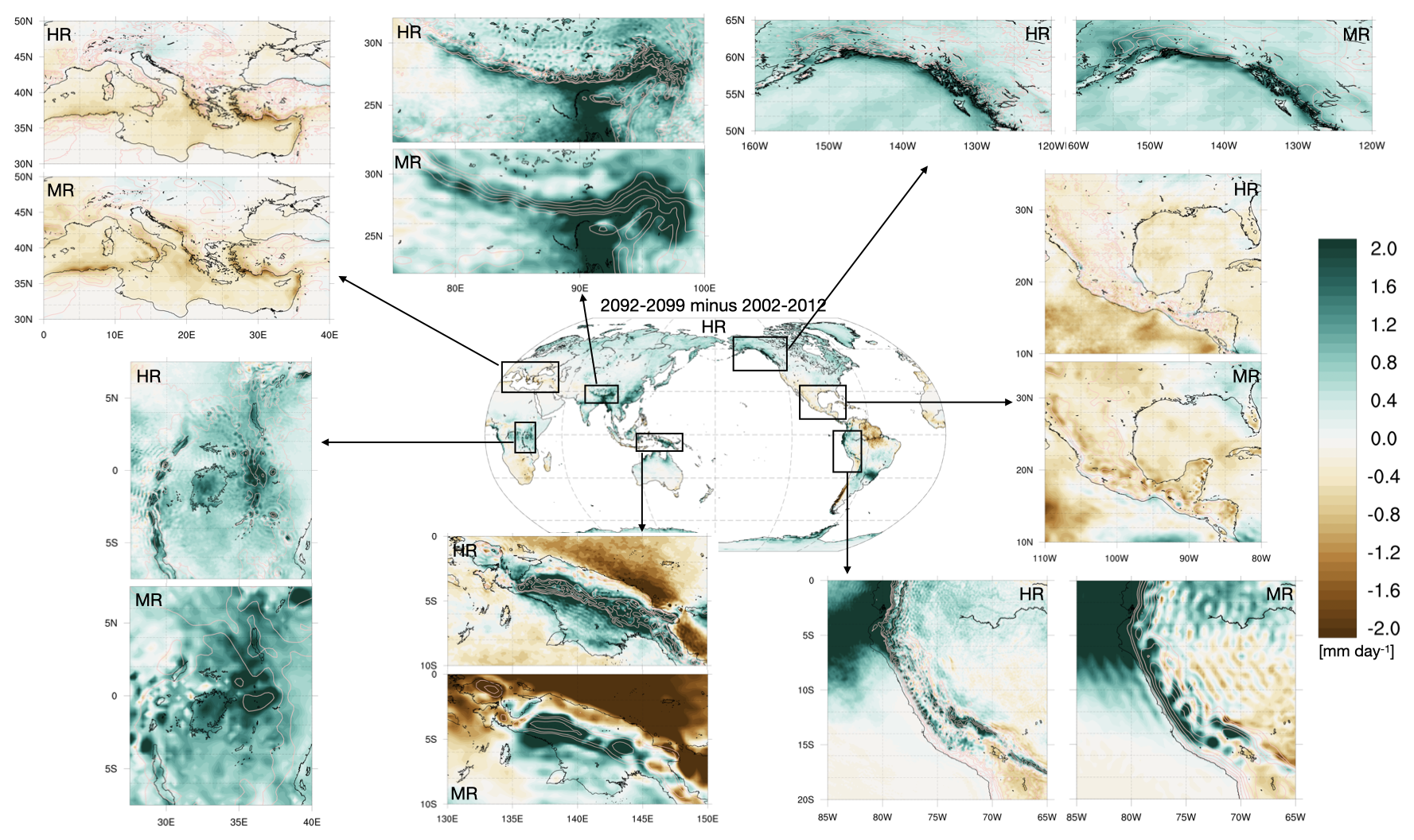
Figure 8 Projected total precipitation changes (mm d⁻¹) from 2002–2012 to 2092–2099 on global (middle) and regional scales in MR and HR resolutions for (clockwise) Mediterranean, Himalaya, Pacific Northwest, Andes, Papua New Guinea, and Victoria Lake regions. The light pink lines represent the elevation of orography at 0.5, 1, 2, 3, and 4 km.

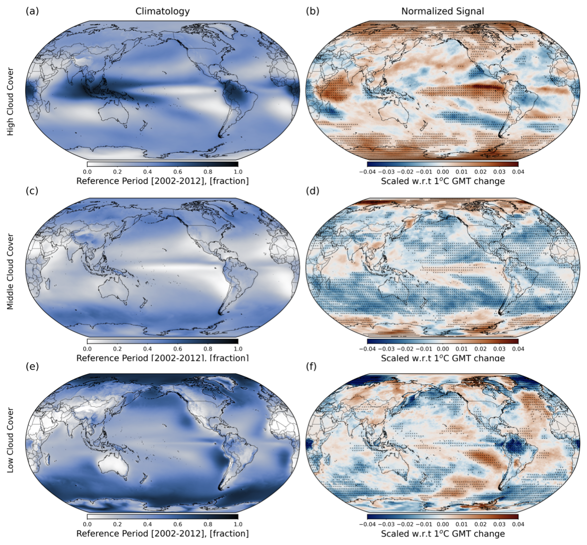
Figure 9 Annual mean cloud climatology of HR simulations during 2002–2012 (a, c, e) and projected climate change signal normalized with respect to a 1 °C global mean temperature change (b, d, f) for (a, b) high, (c, d) middle, and (e, f) low clouds. The stippled areas indicate areas where the null hypothesis can be rejected at the 95 % confidence level using Welch's t test. We used the default settings in the stats module SciPy (version 1.11.1) in Python, which applies Welch's t test at every grid point allowing for unequal variances.

On a global scale, MR and HR simulate a global decrease in low- and middle-level clouds and an increase in the upper-level clouds (Figs. 9, S5) in response to the SSP5-8.5 greenhouse forcing. The former contributes to an increase in incoming shortwave radiation and the latter accelerates the greenhouse effect by emitting longwave radiation at a higher altitude, which corresponds to a reduction in outgoing longwave radiation (OLR). Taken together, the vertical shifts in clouds provide a positive feedback for greenhouse warming.

On a more regional scale, one of the most striking features is the reduction in low and high clouds (> 5 % °C⁻¹ global mean temperature (GMT) change) over the tropical rainforest regions, in particular the Congo Basin and Amazonia (Fig. 9b, d). Interestingly, over central Africa this trend is not mirrored by a corresponding regional drying trend, which hints at a much greater future rainfall efficiency (Almazroui et al., 2020). High clouds increase particularly in the central to eastern Pacific and in polar regions, where they can also contribute to the greenhouse effect, as well as in the western United States, South China Sea, East China Sea, and the western Indian Ocean. The overall structure of the cloud response is qualitatively consistent with high-ECS CMIP6 model simulations (Bock and Lauer, 2024), which further illustrates the robustness of our simulation on regional and planetary scales.

To further elucidate the atmospheric circulation changes and the corresponding cloud-radiative feedbacks, it is necessary to understand the underlying patterns in projected SST (Fig. 10a, b). The model simulates an enhanced equatorial warming (EEW) with a slightly weaker western Pacific warming compared to the east. This EEW pattern can be explained in terms of the weak climatological wind speeds along the Equator (Fig. 7c), the associated weak evaporative cooling feedback (Murtugudde et al., 1996), and the corresponding weaker Walker circulation (Fig. 7d), which further reduces eastern equatorial upwelling, thereby contributing to the warming tendency. The EEW also leads to strong wind convergence along the Equator, further weakening the wind speed and the evaporative feedback. Additionally, it intensifies deep convection, which increases the fraction of high clouds (Fig. 9b), enhances precipitation along the Equator (Fig. 7f), and reduces surface ocean salinity (Fig. 10d), in accordance with recent studies (Kim et al., 2023). Along with the increased temperatures, reduced salinities and equatorial wind speeds, the mixed-layer shoals (Fig. 10f), which in turn also increases the response of temperatures to atmospheric heat fluxes. Furthermore, the reduced mixed-layer depth in the equatorial Pacific and the associated increased stratification lead to a weakening of the zonal pressure gradient along the Pacific (Kim et al., 2023), which also boosts the eastern equatorial Pacific warming.

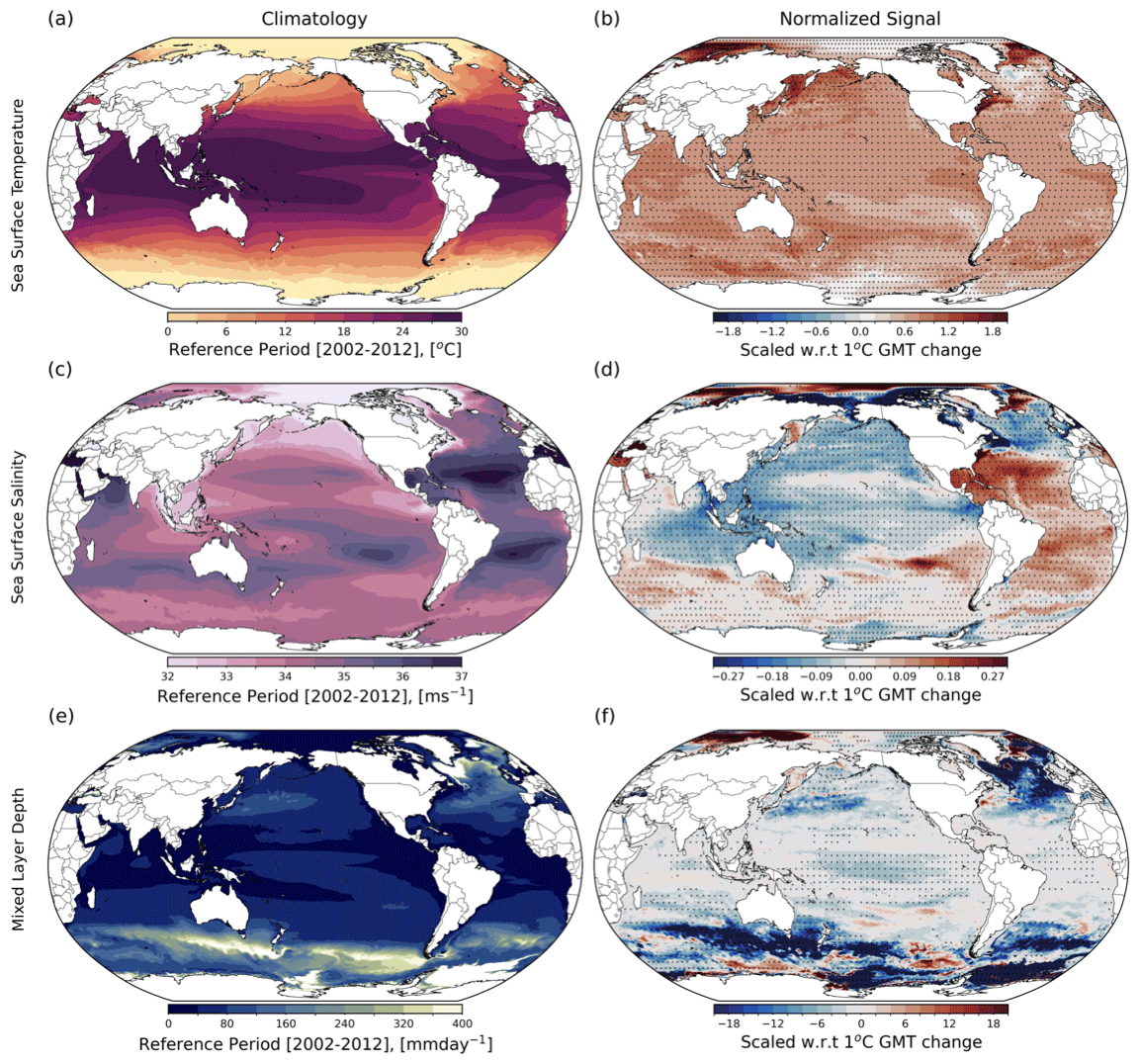
Figure 10 Annual mean climatology of ocean variables in HR simulations during 2002–2012 (a, c, e) and projected climate change signal normalized with respect to a 1 °C global mean temperature change (b, d, f) for (a, b) sea surface temperature, (c, d) sea surface salinity, and (e, f) mixed-layer depth. The stippled areas indicate areas where the null hypothesis can be rejected at the 95 % confidence level using Welch's t test. We used the default settings in the stats module SciPy (version 1.11.1) in Python, which applies Welch's t test at every grid point allowing for unequal variances.

Accelerated future ocean warming can also be found in the Barents–Kara seas and the western side of the northern hemispheric subpolar gyres and along the northern edge of the Antarctic Circumpolar Current (Fig. 10b), which can be linked to a retreat in sea ice. The presence of a weak simulated “warming hole” (0.1 °C 1 °C⁻¹ GMT) in the North Atlantic subpolar gyre which is qualitatively consistent with observations and other model results (Caesar et al., 2018; Keil et al., 2020) can be linked in part to (i) a reduction in the poleward heat transport due to a weakening of the Atlantic Meridional Overturning Circulation (AMOC) (Fig. S6) and (ii) a weakening of deep winter convection south of Greenland and a regional shoaling of winter mixed layers (Fig. 10f), which increases the efficiency of winter-heat-flux-driven cooling of the ocean.

The simulated differences in upper-ocean salinity also reveal an overall increase in Atlantic Ocean salinity, in particular in the subtropical regions, and a reduction in the Pacific, which implies that there is increased freshwater transport from the Atlantic to the Pacific, likely through the climatological mean trade wind export of increased water vapor concentrations from the tropical Atlantic across the Central American isthmus (Richter and Xie, 2010). The freshening in the subpolar North Atlantic and along the Arctic coast reflects the intensification of the hydrologic cycle in the Northern Hemisphere (Carmack et al., 2016), which increases precipitation and river runoff at high latitudes (Fig. 7f). Moreover, a weaker AMOC (Fig. S6) would also reduce the poleward salinity transport due to the positive salinity feedback (Stommel, 1961), which can lead to an accumulation of salinity (Krebs and Timmermann, 2007) in the subtropical North Atlantic and a freshening of the subpolar latitudes, in accordance with Fig. 10d.

Compared to coarser-resolution CMIP5 and CMIP6 models, our MR and HR simulations exhibit many more small-scale current features, such as zonal jets in the subtropical oceans (Maximenko et al., 2008; Richards et al., 2006), the Antarctic Circumpolar Current region, and the Oyashio region (Fig. 11a). The high-resolution ocean model (Fig. 3c) allows us further to resolve small-scale ocean currents such as the Hawaii Lee Counter Current west of the Big Island (Xie, 1994; Sasaki et al., 2010; Lumpkin and Flament, 2013) or the Costa Rica Dome, which is spun up by the strong well-resolved cyclonic wind-stress curl associated with the Tehuantepec and Papagayo wind jets (Fig. 7c), and the Galapagos wake effect of the South Equatorial Current (Eden and Timmermann, 2004) (Fig. 6).

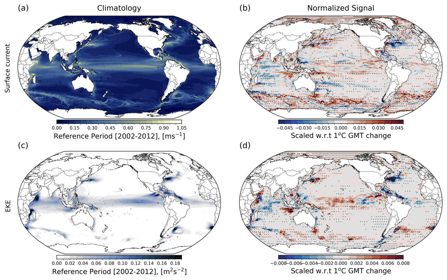
Figure 11 Annual mean climatology of HR simulations during 2002–2012 (a, c) and projected climate change signal normalized with respect to a 1 °C global mean temperature change (b, d) for (a, b) upper-ocean current speed and (c, d) eddy kinetic energy. The stippled areas indicate areas where the null hypothesis can be rejected at the 95 % confidence level using Welch's t test. We used the default settings in the stats module SciPy (version 1.11.1) in Python, which applies Welch's t test at every grid point allowing for unequal variances.

Linked to the changes in winds (Fig. 7d) and buoyancy forcing (Fig. 10b, d) are also changes in upper-ocean currents (Fig. 11b) and their instabilities and generated changes in eddies (Fig. 11d). The simulated future changes in ocean currents and eddy kinetic energy (EKE) are more prominent in regions where the currents and eddies are already energetic in the historical simulation (Fig. 11a, c). The HR model simulates a gradual slowdown of the South Equatorial Current, which is consistent with the overall weakening of the equatorial trade winds (Fig. 7d). In the Southern Ocean the northern branch of the Antarctic Circumpolar Current and the Antarctic Slope Current intensify. Furthermore, we observe a gradual strengthening and northward shift in the Kuroshio Current, as evidenced in both the surface current and EKE, consistent with the observed trend (Yang et al., 2016). The Gulf Stream, and North Atlantic Drift and the associated EKE weaken in the future, which can be linked to the weakened AMOC, Gulf Stream and North Atlantic Drift in a warming climate (Fig. S6), which would be accompanied by reduced baroclinic and barotropic instabilities. Previous studies found significant correlations between the low-frequency variabilities in the AMOC and EKE, suggesting a linkage also in their future changes (Beech et al., 2022). Both the Antarctic Circumpolar Current (ACC) strength and the EKE in the ACC region are projected to intensify along with the strengthening of the westerly winds in the future (Fig. 7d). This result indicates that the ACC is not in an eddy saturation state in the simulation. The Agulhas Return Current is projected to shift poleward, consistent with the poleward shift in the westerlies. Both the ocean current and EKE will increase off the southwestern coast of Africa in the future, indicating an increase in Agulhas leakage and water mass transport from the Indian Ocean to the Atlantic, which has been linked previously to the poleward shift in the Southern Hemisphere Westerlies (Biastoch et al., 2009) (Fig. 7d). The Brazil and Malvinas currents show a poleward shift, which is further corroborated by observational studies in the region (Drouin et al., 2021). Overall, the projected changes in the large-scale pattern and magnitude of ocean currents and EKE are consistent with previous modeling studies and some inferences from observations (Martínez-Moreno et al., 2021; Beech et al., 2022).

When zooming into specific regions, the HR model 10-year projections provide more detailed information on regional scales, with major changes in currents and EKE occurring, e.g., in the South China Sea, Lombok Strait, and the Mozambique Channel.

With an ocean and sea-ice resolution of about 5–10 km in polar regions, the AWI-CM3 MR and HR simulations are ideally suited to resolve sea-ice processes realistically (Figs. S7, S8, 12). This is further illustrated in the comparison between observations of sea-ice fraction (Lavergne et al., 2019; Lavergne and Down, 2023) (shown here for September and February means) in the Southern Ocean and Arctic Ocean for the 2000s (2002–2012) in the HR simulation (Fig. 12). We find excellent qualitative agreement between observations and model simulations. In particular, the maximum sea-ice extent in February and the minimum in September are well captured in the Arctic Ocean. This is further corroborated by the simulated climatology (Figs. S9, S10). Given the high resolution of the sea-ice model (∼ 5 km in the Arctic Ocean), we can identify additional features that cannot be resolved in coarse-resolution models, such as coastal polynyas around Antarctica, sea-ice eddies, and large-scale cracks (“Video supplement” S2, Moon et al., 2024b). As expected, the sea ice shrinks dramatically in response to greenhouse warming, and by the 2090s (Fig. 12, lower panels, Fig. S8, left), the austral winter sea ice around Antarctica almost disappears, except for a few remaining parts in the western Weddell and Ross seas.

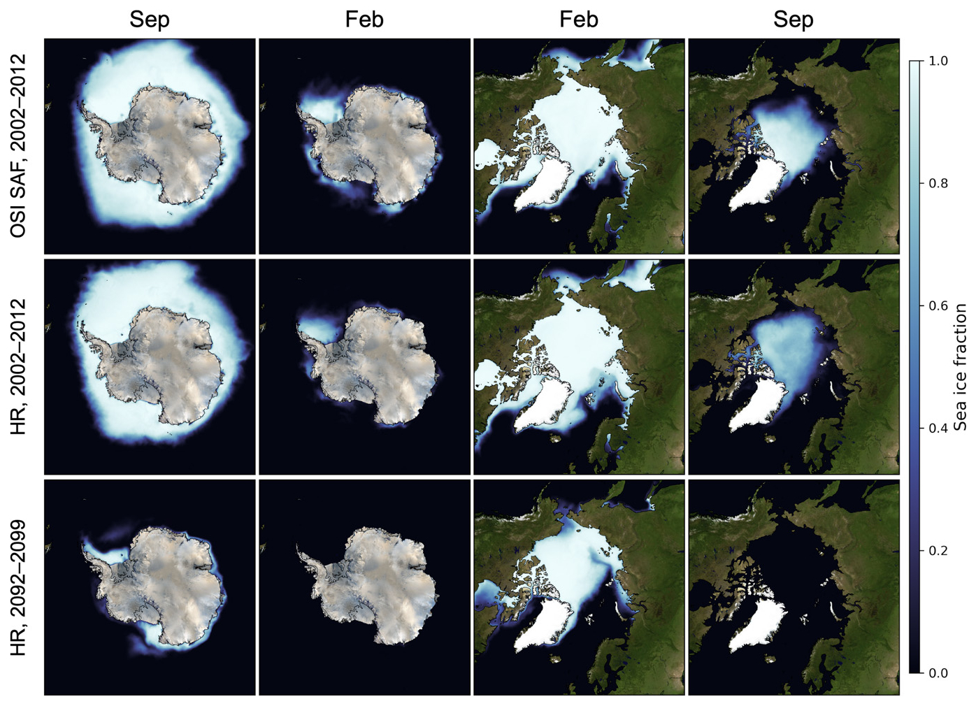
Figure 12 Upper row: monthly means of sea-ice fraction in observations (Lavergne et al., 2019) for 2002–2012 in the Southern Ocean (September and February, left panels) and Arctic Ocean (February and September, right panels). Middle row: same as upper row, but for the HR simulation. Lower row: same as middle, but for 2092–2099.

In the SSP5-8.5 scenario, by the 2060s, the respective summer sea ice will disappear in both hemispheres. Similar to coarser-resolution climate models (Notz and Community, 2020), a substantial amount of Arctic sea ice remains in wintertime in the HR simulation. The Arctic amplification of atmospheric surface temperatures (Fig. 7b) is mostly a wintertime signal associated with winter sea-ice loss, and it can be traced back to the heat accumulation during summer due to sea-ice reduction (Chung et al., 2021). We therefore still see a strong Arctic amplification (Fig. 7b) towards the end of the century in the HR simulation. This effect normally disappears in coupled general circulation models for even higher atmospheric CO₂ concentrations once winter sea ice disappears completely (Chung et al., 2021). The simulated HR sea-ice loss in Arctic regions is also linked with an intensification of the hydrological cycle, more precipitation, and increased middle to high cloudiness (Figs. 7f, 9b, 9d) and a surface wind acceleration due to increased mixing of winds from aloft and reduced surface friction due to reduced sea-ice cover (Fig. 7d).

The oceanic response to declining sea ice in the Southern Ocean is associated with a coastal freshening (reduced brine rejection) (Fig. 10d) and a corresponding geostrophic intensification of the Antarctic Slope Current (Fig. 11b). The sea-ice reduction further contributes to the southward shift in the Southern Hemisphere Westerlies (Russell et al., 2006) (Fig. 7d) and the associated increase in middle to high cloud cover (Fig. 9b, d) as well as precipitation near Antarctica (Fig. 7f).

5 Extremes

One of the key advantages of high-resolution global earth system models is the possibility of resolving mesoscale atmospheric processes, as well as capturing the interaction between large-scale flow and small-scale topographic features, which can lead to the generation of extreme regional climate impacts. Here we focus on the representation of atmospheric extreme events and the projected future changes in the probability distribution of rainfall, heat waves, and tropical cyclones. To document the effect of resolution and greenhouse warming on extreme rainfall, which is arguably one of the costliest impacts of anthropogenic climate change, we compute the probability density functions (PDFs) of the aggregated spatiotemporal rainfall data for the periods 2002–2012 and 2092–2099 (Fig. 13a). The comparison with the ERA5 precipitation data (Hersbach et al., 2023) reveals a slight underestimation for both the MR and HR simulations (2002–2012) of extreme precipitation values between 25–250 mm d⁻¹. We find that for present-day rainfall events larger than 50 mm d⁻¹, HR has a 21 % higher occurrence probability compared to the MR simulation. For future climate conditions the HR–MR difference for extreme precipitation only amounts to 8 %. The climate change response is characterized by an increase in the number of extreme rainfall events (above 50 mm d⁻¹) between 2002–2012 and 2092–2099 by 92 % for MR and 72 % for HR. This demonstrates that (i) storm-resolving models lead to stronger extreme rainfall events and (ii) a warmer climate produces more rainfall extremes, consistent with previous studies (Rodgers et al., 2021; John et al., 2022).

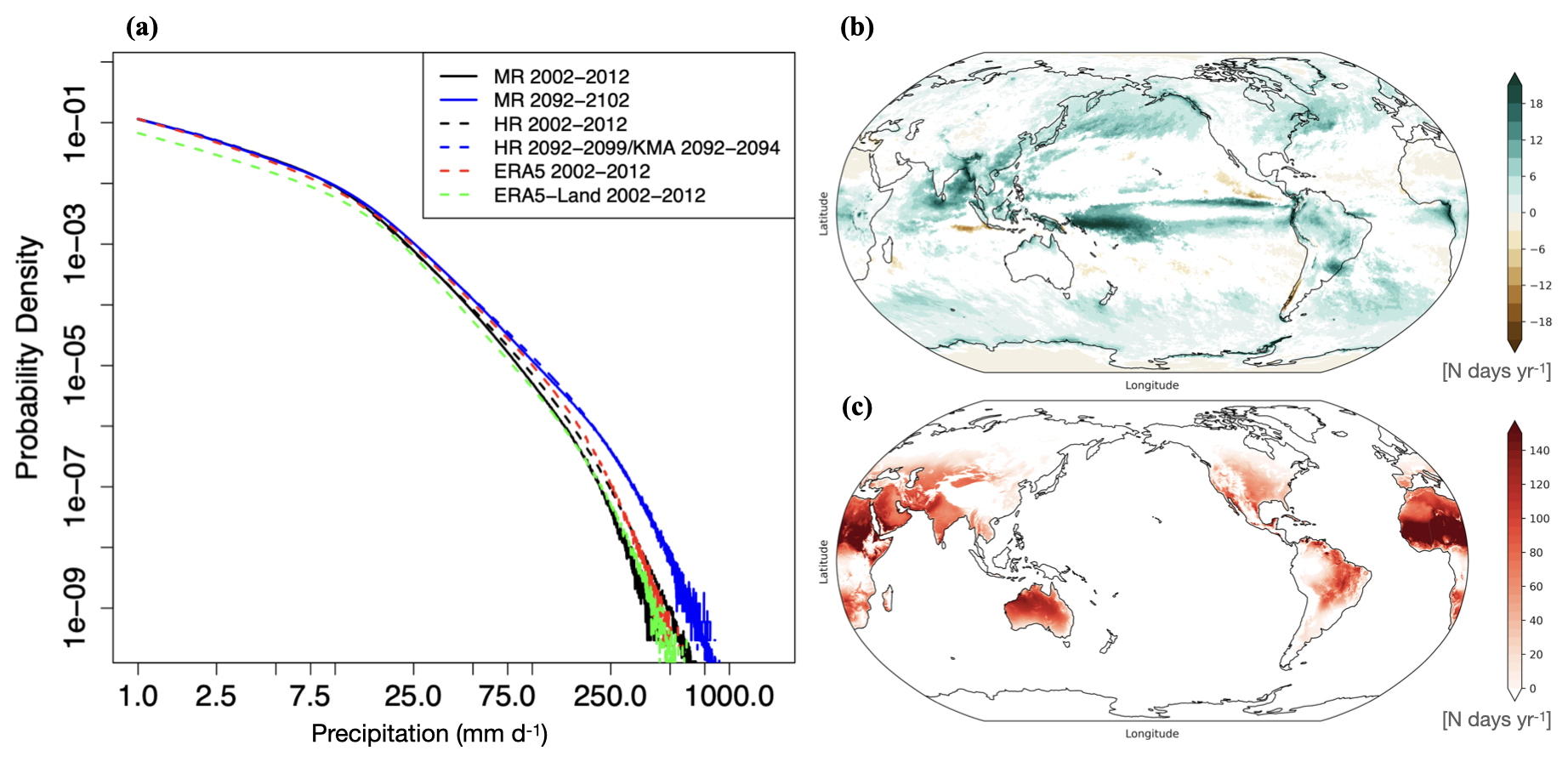
Figure 13 (a) Probability density functions for daily accumulations of precipitation. The significance is checked using the Kolmogorov–Smirnov test, performed with the ks.test() function in R. Solid lines represent MR, and dashed lines represent HR; black lines are for present climate (2002–2012) and blue lines for future climate (2092–2099). Dashed red and green lines correspond to the same analysis for ERA5 total and land precipitation data, respectively (2002–2012). (b) Difference in the average number of days per year exhibiting accumulated daily precipitation of more than 50 mm d⁻¹. (c) Difference in the average number of days when the maximum daily temperature exceeds 40 °C. The difference is computed between the time periods 2092–2099 and 2002–2012, and shadings indicate statistically significant difference at the 95 % confidence level by Welch's t test. We used the default settings in the stats module SciPy (version 1.11.1) in Python, which applies Welch's t test allowing for unequal variances.

In Fig. 13a, there is also an indication for different scaling behavior for accumulated precipitation up to 10 mm d⁻¹, for accumulated precipitation between 10 and 300 mm d⁻¹, and for larger accumulations. Similar scaling regimes have been found previously (Yang et al., 2020) for station data in an extreme value analysis. This suggests that different mechanisms might be responsible for creating precipitation events of different magnitudes.

Next, we examine the change in the numbers of days per year above certain impact thresholds (Fig. 13b, c). For precipitation we choose the threshold for very heavy precipitation (> 50 mm d⁻¹ based on the World Meteorological Organization definition). Consistent with previous studies (Pfahl et al., 2017; Rodgers et al., 2021), we find that the large-scale monsoon and ITCZ systems, as well as the areas affected by the major storm tracks, are projected to have more frequent very heavy rainfall events by 2090. In addition, we find an intensification in the number of extreme precipitation days across eastern Asia (5–20 d more), Papua New Guinea, Oceania, Amazonia, and central and western Africa. Moreover, the HR model simulates a strong intensification in the frequency of extreme rainfall along steep topographic slopes, e.g., Kilimanjaro, Norway, the southeastern side of the Himalayas, and the Andes. These will likely increase landslide hazards with impacts on local communities who live downslope from these extreme precipitation hotspots (Kirschbaum et al., 2020).

For the SSP5-8.5 greenhouse gas emission scenario, the number of days exceeding 40 °C maximum daily temperatures increases dramatically equatorward of 40 ° latitude, with some areas, e.g., Pakistan, eastern India, parts of Amazonia, northern central Australia, northern and southern Africa, and the Arabian Peninsula, projected to have at least 100 d yr⁻¹ more (compared to the present day) exceeding this extreme temperature by the 2090s. In Europe, the Mediterranean will be most affected, and over North America, California and the Great Plains region develop as hotspots. The changes over the Maritime Continent are quite small, highlighting the role of negative evaporative land-surface feedbacks and the effect of reduced high clouds (Fig. 9b), which reduces regional longwave warming.

Accurate simulation of tropical cyclones is crucial for understanding their global impacts, including human and economic losses, and for assessing regional risk and preparedness. Modeling tropical cyclones presents several challenges due to their small size, occurrence at variable distribution tails, and significant variability in both time and space (see inlays in Fig. 6, “Video supplement” S5, Moon et al., 2024b). To evaluate the model's ability to represent the global spatial distribution, annual cycle, and wind speeds associated with tropical cyclones, we employed the Okubo–Weiss zeta parameter (OWZP) tracking scheme, which is a resolution-independent method for detecting the genesis and tracks of tropical cyclones (Tory et al., 2013a, b). The detailed methodology can be found in the Supplement.

One key limitation of climate models in representing tropical cyclones is the significant underestimation of maximum 10 m wind speed, even when employing models with kilometer-scale resolution (Fig. S9). The simulation using the MR configuration fails to capture tropical cyclones at category 2 or higher on the Saffir–Simpson scale. The same issue persists when the OWZP tracking is applied to the ERA5 reanalysis dataset, which shares a similar resolution with the MR simulation. The issue of wind underestimation was previously observed during a multi-model comparison in horizontal grid spacing ranging from 250 to 25 km, where models were found to be incapable of accurately representing highly intense surface wind speeds, while the minima of surface pressure were represented well (Roberts et al., 2020a, b). The HR simulation at scales of 9 km exhibits better performance compared to the MR simulation, as indicated by the peak of the PDF at the tropical storm strength (wind speeds greater than 17 m s⁻¹) at around 25 m s⁻¹, similar to observed values (Fig. S9). The secondary peak of observations at the category 4 level in the wind speed probability distribution is associated with the tropical cyclones that undergo rapid intensification, characterized by significant increases in wind speed within a short period of time (Lee et al., 2016). The MR present-day simulation fails to generate rapid intensification, whereas in the HR simulation 13 cases are identified over 13 years (simulated year of 2000–2012), although their maximum wind speeds still remain below category 3 levels.

In spite of the limitations in tropical cyclone wind intensity simulations (an issue which was resolved by modifying the Charnock parameter in later cycles of the IFS model) (Bidlot et al., 2020; Majumdar et al., 2023), the HR simulation effectively captures the spatial distribution and annual cycle of tropical cyclones (Fig. 14). The total number of tropical cyclones per year in the present-day simulation is 83.8, a value that exactly matches the observed number of 83.8. In general, the model tends to overestimate tropical cyclone activities in the western North Pacific and southern Indian Ocean, while it underestimates them in the North Atlantic. The underestimation of Atlantic hurricane activities has been a long-standing issue observed across various models, from low-resolution CMIP5 models (Camargo, 2013) to medium-resolution models (Roberts et al., 2020b), particularly when coupled with ocean models. In our HR simulation, the underestimation may be further amplified by the negative SST bias in this area (Figs. 5, S4). The seasonal cycle of tropical cyclone frequency in each basin is represented well in the model as compared to the IBTrACS4 observational product (Knapp et al., 2010), with a large number occurring during their respective major tropical cyclone season (Fig. 14, lower panels). There is a 1-month delay in their peak activity month, especially in the eastern Pacific, whereas the North Atlantic exhibits a peak activity 1 month earlier than observed. To understand the shift in the peak tropical cyclone (TC) activity month, we have examined the seasonal cycle of environmental conditions that are favorable for TC genesis, including sea surface temperature (SST), relative humidity at 700 hPa (R700), and vertical wind shear between 200 and 850 hPa (VWS) (Fig. S10). The seasonal cycle of these variables matches very well with observations in most of the basins. However, over the eastern Pacific basin, there is an overestimation of SST and R700 and an underestimation of VWS in late summer (September–October), which together provide favorable conditions for TC genesis. Therefore, the 1-month delay in TC peak activity can be explained by the more favorable conditions that our model simulates. In contrast, the North Atlantic basin SST and R700 are underestimated throughout the seasons. This may act to reduce TC genesis over the North Atlantic during the entire year. However, considering that the majority of TCs in the Atlantic basin originate from tropical easterly waves, further analysis is required to understand whether there is any underestimation of easterly wave activity or its coupling to TCs. Despite this 1-month offset, the model generally captures the seasonal cycle of global tropical cyclone activity very well.

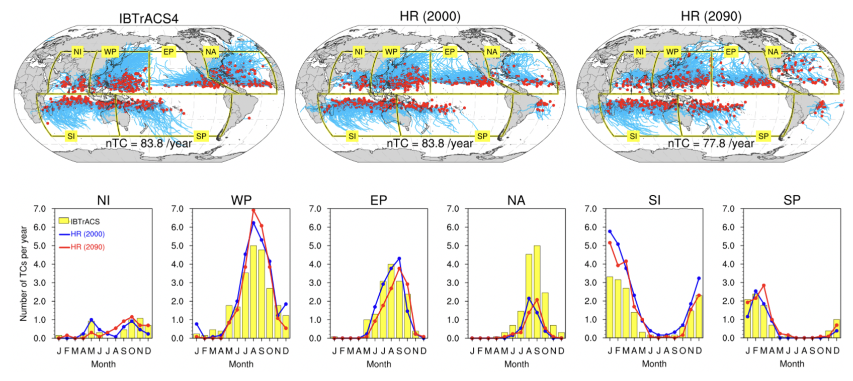
Figure 14 Tropical cyclone tracks for present-day and future conditions: tropical cyclone tracks from (a) the observation (i.e., IBTrACS4) (years 2000–2012) and those identified by the resolution-independent OWZP tracking scheme for (b) present-day simulations (13 years for HR 2000 chunk) and (c) respective future conditions (13 years for HR 2090 chunk). (d–i) Annual cycle of tropical cyclones for each basin.

To gain further insights into the impact of greenhouse warming on tropical cyclone activity, we conducted an analysis of the 2090–2099 CE HR simulation (Fig. 14). In the HR global warming simulation, the projected changes indicate a global reduction in tropical cyclone frequency by approximately 7 %. This reduction in global tropical cyclone frequency primarily occurs in the eastern Pacific and southern Indian Ocean. In contrast, the changes in other basins either are negligible (e.g., South Pacific) or show a slight increase (e.g., north Indian and South Pacific oceans). Interestingly, we find a zonal asymmetry across the western Pacific, with decreased frequencies in the western part and increased occurrences in the eastern part of the western Pacific (figure not shown).

Several previous studies agree that the overall frequency of tropical cyclones will decrease in response to global warming, while strong tropical cyclones are likely to become more intense in the future (Knutson et al., 2015; Chu et al., 2020; Roberts et al., 2020b). Our results contribute to this understanding and provide robust insights into potential changes in tropical cyclones from a high-resolution coupled modeling perspective. However, further research is needed to better comprehend the impact of high-resolution grid spacing and wind speed biases on accurately representing the dynamics and structures of tropical cyclones, such as double-eye walls and rain bands (Fig. 6, inlay); cyclone mergers (“Video supplement” S5, Moon et al., 2024b); and the physical mechanisms underlying their future changes.

6 Modes of climate variability

Our 20-year HR control simulation and the 10-year transient greenhouse warming segments (15 years for 2090 chunk, including the simulations run on the KMA computer GURU) allow us to assess the performance of important large-scale modes of climate variability, determine their regional characteristics, and identify potential future changes. Here we focus on (i) the MJO (Zhang, 2013), a major mode of tropical variability with a timescale of 40–90 d; (ii) the North Atlantic Oscillation (NAO) (Visbeck et al., 2001; Hurrell and Deser, 2009), which plays a key role in interannual fluctuations in European winter climate; and (iii) the El Niño–Southern Oscillation (ENSO), known as the leading mode of interannual global climate variability (Timmermann et al., 2018). Again, here we can only give a very brief overview of some of the main projected changes in climate variability without any in-depth mechanistic explanations. This shall be left for future studies.

6.1 Madden–Julian oscillation

Even though the MJO explains a considerable fraction of variance in the tropics on intraseasonal timescales, it has remained notoriously difficult to simulate in coarser-resolution CMIP-type coupled general circulation models (Ahn et al., 2020; Le et al., 2021; Chen et al., 2022). Model performance in the eastward propagation of the MJO is improved in CMIP6 models compared to CMIP5 models (Ahn et al., 2020; Li et al., 2020), but MJO variability is still underestimated in most CMIP6 models (Le et al., 2021). Here, we examine the skill of MR and HR in simulating the MJO based on the wavenumber–frequency diagram of daily OLR averaged over 10° S–10° N and for the months from November to April (NDJFMA) when the MJO activity is strong. In the observations, a prominent peak occurs for eastward-propagating OLR anomalies with wavenumber 1–3 contributions and for periods of 40–90 d (Fig. 15a). The MR and HR simulations qualitatively capture these features, although the spectral peak occurs for periods of 70–80 d (Fig. 15b, c). We further explore the wavenumber–frequency spectra using observed and simulated daily precipitation (Fig. S11). CMIP5 models (Ahn et al., 2017) show a diverse range of spectral power across broader periods and wavenumbers, and CMIP6 models exhibit large inter-model spread in MJO simulation skills. Although the spectral amplitudes in both HR and MR simulations are weaker compared to the observations, our simulations show good MJO performance, with a relatively low root mean squared error in the spectral domain. These results indicate that the representation of the MJO in our simulations is fairly realistic compared to the majority of the CMIP6 models. This encourages us to further study the response of the MJO to SSP5-8.5 greenhouse gas forcing (Fig. 15d, e). In both MR and HR future simulations (2090–2099), the MJO peak splits into two peaks. One peak characterizes low-frequency (> 90 d) OLR variability, while the other is a pronounced 35–40 d peak. The intraseasonal signals in the power spectra are projected to increase relative to the present-day simulations, indicating an enhancement of faster eastward-propagating signals (Chang et al., 2015). Similarly, future enhancements in both low-frequency and intraseasonal peaks in precipitation are observed in some models, including CESM2, CNRM, and NorESM2 (Fig. S12). It has been suggested that the MJO power may shift towards higher frequencies with increasing global warming (Cui and Li, 2022). Unraveling the underlying mechanisms responsible for the projected MJO changes and narrowing down the remaining uncertainty in its sensitivity to greenhouse warming are beyond the scope of our study.

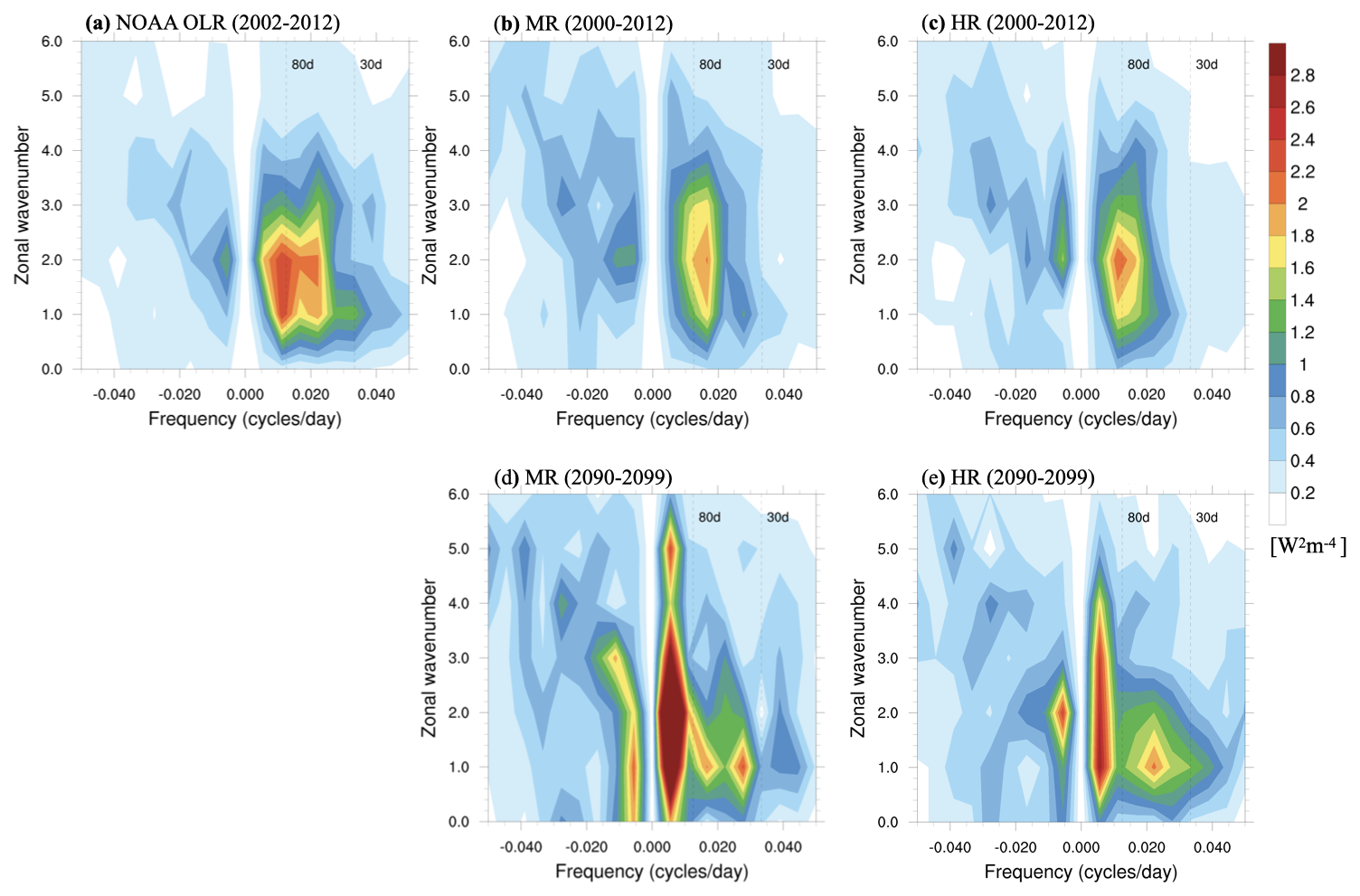
Figure 15 Wavenumber–frequency diagram of outgoing longwave radiation (OLR) during NDJFMA, 2000–2012, between 10° S–10° N for observations (NOAA PSL, 2024) (a), MR 2000–2012 (b), HR 2000–2012 (c), MR 2090–2099 SSP5-8.5 (d), and HR 2090–2099 SSP5-8.5 (e). Frequency unit is cycles d⁻¹, and OLR shading is in W² m⁻⁴.

6.2 North Atlantic Oscillation

Year-to-year changes in winter climate over Europe with important socio-economic consequences are primarily controlled by the leading mode of atmospheric variability over the North Atlantic sector, which is commonly known as the NAO (Wanner et al., 2001; Hurrell and Deser, 2009). Here we focus on some of the regional features of the NAO simulated by MR and HR, which are usually absent in large-scale assessments of NAO impacts (Hurrell and Deser, 2009). The NAO-related winter variability signal over Europe with topographically induced fine-scale features can be captured in nested regional climate simulations, but models with a relatively coarse resolution have limitations in exhibiting regional-scale signals (Bojariu and Giorgi, 2005). The local aspects of the NAO are particularly relevant for stakeholders (e.g., vineyards in Rhône River valley or farmers in Georgia), and our simulations may help in mitigating negative impacts associated with extreme NAO phases (Dawson and Palmer, 2015) in sectors such as agriculture, energy generation, water management, and wildfire prevention.

Here, the NAO index is defined as the principal component (PC) time series of the leading empirical orthogonal function (EOF) of winter (DJF) sea level pressure (SLP) anomalies over the Atlantic sector (20–70° N, 90° W–40° E) (Hurrell and Deser, 2009). A positive NAO index is characterized by stronger westerlies over the North Atlantic and Europe, the advection of warmer marine air across Europe, the drying of the Mediterranean, and the increased rainfall over northern Europe (Visbeck et al., 2001). We focus on the impact on regional precipitation and wind speed, both of which are relevant for hydropower and wind-power generation (Jerez et al., 2013), as well as on surface temperature. Compared with the MR case (Fig. 16b, e), which shows the general windy and wet–dry meridional dipole across Europe for a positive NAO index, the HR simulation (Fig. 16b, c, f) shows topographically even more pronounced responses, in particular on the western side of Norway and Scotland (wet); the Atlas mountains (dry); the Rhône River valley (dry); and the western side of the Mediterranean mountain ranges (drying), such as the Apennines, the Denaric Alps, Pyrenees, and Pindus. This illustrates that the changes in surface westerlies and associated moisture transport with steep topography extend much further east than commonly assumed, creating important regional impacts that may be relevant for agriculture and other sectors. In the positive NAO phase, northern Europe is more likely to experience much warmer conditions in the HR simulation compared to the MR simulation. In addition, in the HR simulation, the temperature response over Italy to the NAO phase shows a clear division between northern-central and southern Italy, with warmer conditions in northern-central Italy during positive NAO phases. This finding is consistent with ERA5 between the NAO index (Fig. 16a, d) and temperature anomalies (Fig. 16g), as well as the observed correlation at thermometer stations (Gentilucci et al., 2023). In contrast, this feature is absent in the MR simulations. It should be further noted that the precipitation and wind responses over Türkiye and temperature response over Portugal and Spain to the NAO phase are quite different in the HR simulation.

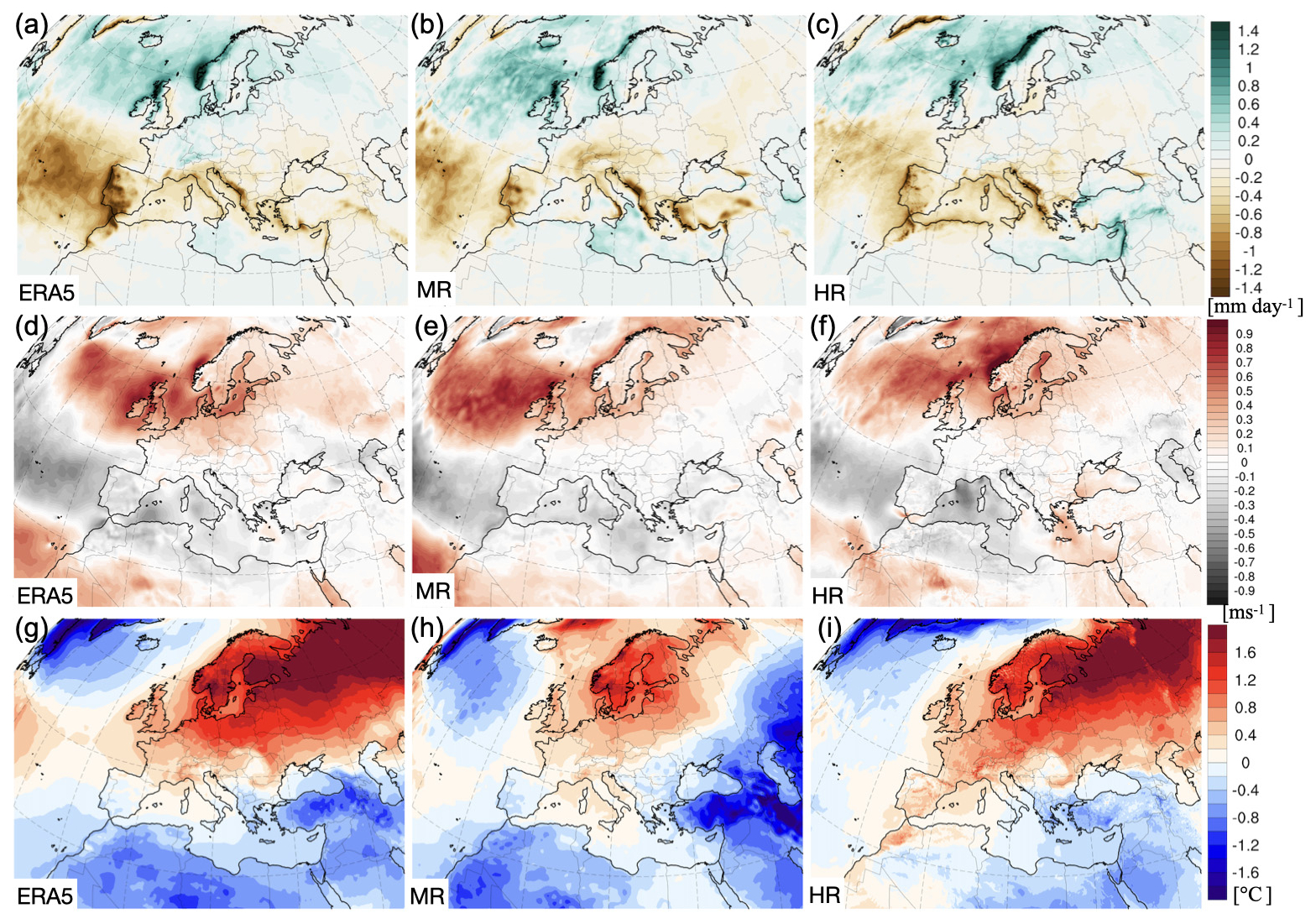
Figure 16 Precipitation (mm d⁻¹) regression with North Atlantic Oscillation index using 20 years (2000–2019) of the ERA5 reanalysis (a) and 13 years (2000–2012) for the MR simulation (b) and HR simulation (c). Panels (d), (e), and (f), same as (a), (b), and (c), but for the wind speed (m s⁻¹). Panels (g), (h), and (i), same as (a), (b), and (c), but for the surface temperature (°C). The NAO index is based on the leading empirical orthogonal function of DJF seasonal mean sea level pressure anomalies over the North Atlantic and is normalized.

Changes in atmospheric circulation over the North Atlantic in response to greenhouse warming may induce notable regional changes in weather and climate. For the future positive phase of the NAO, wet conditions on the western side of Norway and dry conditions in Portugal are apparent in both MR and HR simulations (Fig. S13) (McKenna and Maycock, 2022).

6.3 El Niño–Southern Oscillation

To assess the effect of resolution (MR to HR) on the El Niño–Southern Oscillation (ENSO), its climatic impacts, and their projected changes, we first compare the SST anomaly standard deviation in the boreal winter season (DJF) between the observations and the different simulations (Fig. 17). Compared to the observations during the satellite era, both the MR and HR versions simulate the ENSO variability center over the equatorial central-eastern Pacific well, with slightly less ENSO SST variability in the HR control compared to the MR control (Fig. 17a, b, c). It should be noted here that both model versions simulate larger-than-observed SST variability in the extra-tropical eddy-rich regions around the Kuroshio–Oyashio Extension, the Gulf Stream, and the Agulhas. ENSO variability is characterized by a seasonal amplitude modulation of eastern to central equatorial Pacific SST anomalies (Stein et al., 2014). Both MR and HR simulations can reproduce this key feature, albeit with a notable phase bias in the MR simulations, exhibiting a seasonal minimum SST variability in early boreal summer instead of the boreal spring season seen in the observations and the HR simulations (Fig. 17f, g, h). In response to greenhouse warming, the MR configuration shows a large increase in ENSO variability for all months, whereas the HR configuration simulates only a modest increase during the JFM season (Fig. 17d, e).

Figure 17 El Niño–Southern Oscillation variability and its projected changes. Upper row: standard deviation of DJF mean SST anomalies for observations (OISSTv2) (a), the MR 1950 control simulation (b), and the HR 1950 control + 2000 simulations (33 years in total) (c). Middle row: same as upper row (b) and (c), but for the 2090 time slice (15 years in total). Lower row: seasonal standard deviation of Niño 3.4 SST anomaly in observations (OISSTv2) (f), MR (control, gray; 2080–2099, red) (g), and HR (control, gray; 2090–2099, red) (h). Dashed boxes in (a)–(e) enclose the Niño 3.4 region.

The most striking effect of different model resolutions can be seen in ENSO's global impacts at the local scale; i.e. we find that increased resolution (HR vs. MR) translates into pronounced regional granularity in precipitation anomalies due to ENSO teleconnections (Fig. 18a, b, c). For instance, HR simulates a clear meridional tripolar pattern in ENSO-associated precipitation anomalies over the west coast of North America, which is absent in MR. The GPCP rainfall data do not show the tripole structure (Fig. 18a), but the longer-term GPCC compilation of terrestrial rainfall does (Fig. S14). Furthermore, both the positive and negative precipitation anomalies are highly amplified in HR compared to MR, especially over steep orography (Fig. 18c). This has critical implications: ENSO's impacts at the local scale are severely underestimated at model resolutions that are typically used to assess these. Hence, it is imperative to re-evaluate ENSO's various global impacts using kilometer-scale models to provide robust climate risk assessments. Another example of the granularity of ENSO's local impact and their pronounced amplification over mountainous terrain in the HR simulation can be seen for the Maritime Continent region (Fig. 18d, e, f). The MR and HR simulations again exhibit very different patterns of ENSO-associated precipitation anomalies. The effect of resolution on these impacts is exemplified for instance by the simulated drying over the high orography of the Lesser Sunda Islands (Bali, Lombok, Sumbawa, Flores, Sumba, and Timor) during El Niño in HR. In contrast, the MR simulation exhibits slight moistening during El Niño events.

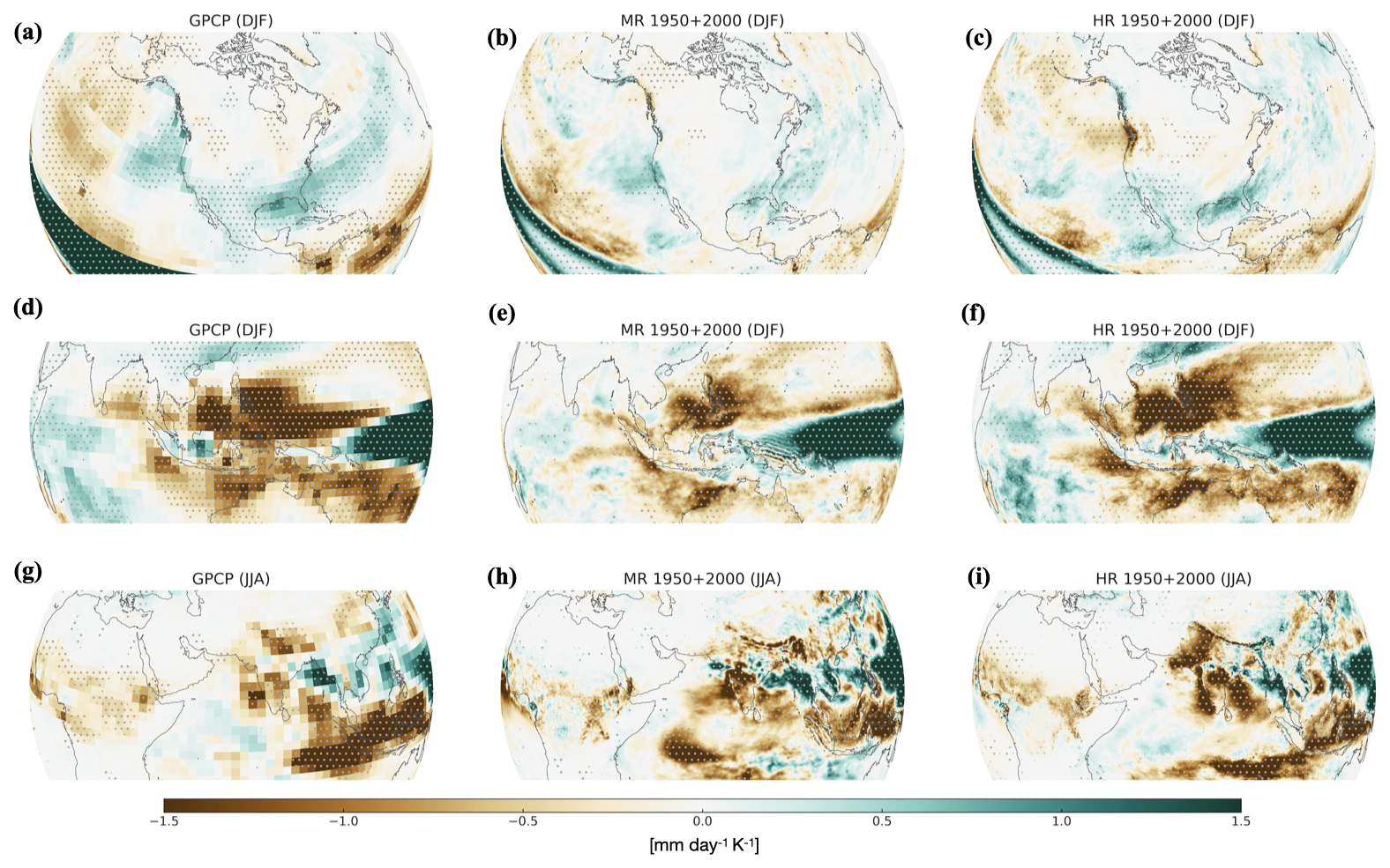
Figure 18 Present-day observed and simulated El Niño teleconnections: regression between DJF Niño 3.4 SST anomalies with GPCP rainfall observations over North America (a) and Maritime Continent (d) (mm d⁻¹ °C⁻¹) and JJA Niño 3.4 SST anomalies with GPCP rainfall observations over Indian Ocean (g). Panels (b), (e), and (h), same as (a), (d), and (g), but for 32 combined years of the MR simulation. Panels (c), (f), and (i), same as (a), (d), and (g), but for 32 combined years of the 1950 and 2000 HR simulations. The data were linearly detrended prior to the analysis. The stippled areas indicate the regression coefficient values that exceed the 90 % confidence level based on a two-tailed Student's t test (against zero regression). We used the stats module package in Python to perform a two-tailed Student's t test, assessing whether the regression coefficients differ significantly from zero.

Future changes in ENSO teleconnections (Figs. S15, S16) indicate that on average ENSO's impact on hydroclimate anomalies is likely to intensify with greenhouse warming. This effect is particularly pronounced in DJF in the HR simulations over Europe (Fig. 19d) but also in the MR transient simulation (Fig. 19b). Under present-day conditions the ENSO linkage to DJF climate over Europe is detectable but quite weak (Fig. 19a) (Fraedrich, 1994; Pozo-Vázquez et al., 2001; Brönnimann, 2007). Increasing temperatures, shifts in the tropospheric and stratospheric circulation, and the overall enhanced availability of water vapor in a warmer climate can intensify the linkage to Europe with El Niño conditions creating wetter (drier) conditions over southern (northern) Europe. Future El Niño events are expected to generate a much larger tropical Pacific rainfall response (Cai et al., 2018). This in turn can strengthen the Pacific subtropical jet and its extension into the Atlantic, as well as create a troposphere-stratosphere bridge, that can influence circulation and rainfall patterns over Europe (Fereday et al., 2020). The latter is particularly pronounced in climate models that resolve stratospheric dynamics with enough vertical resolution, such as the AWI-CM3 model used here with 137 vertical levels. Changes in ENSO rainfall teleconnections are also noticeable in other regions, such as in DJF over southern Africa, eastern China, Japan, and the Korean Peninsula, as well as in JJA over the central Pacific, the Maritime Continent, southern Japan, and along the Andes (Figs. S15, S16), which also show a pronounced future drying in response to El Niño events.

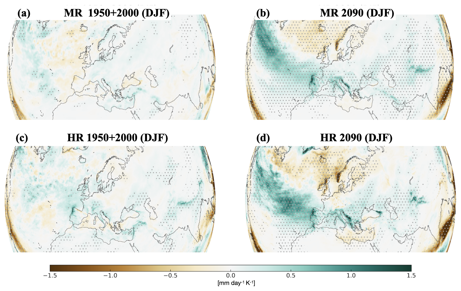
Figure 19 Future changes in El Niño teleconnections to Europe in DJF: regression between DJF Niño 3.4 SST anomalies with detrended simulated rainfall data over Europe (mm d⁻¹ °C⁻¹); (a, c) for the present-day conditions (20 years of 1950 simulation and 13 years from 2000 chunk) for MR and HR resolution; (b, d), same as (a, c), but for 2090 CE climate conditions (using 15 years). The stippled areas indicate the regression coefficient values that exceed the 90 % confidence level based on a two-tailed Student's t test (against zero regression). We used the stats module package in Python to perform a two-tailed Student's t test, assessing whether the regression coefficients significantly differ from zero.

7 Summary and discussion

In this study, we presented a new iterative method for conducting storm-resolving, fully coupled global warming simulations under various future conditions. Our approach involves a medium-resolution (MR) transient simulation with a 31 km atmospheric resolution and a 4–25 km ocean resolution, adopting the SSP5-8.5 scenario forcing. This is followed by a series of 10-year transient high-resolution (HR) time-slice simulations with a 9 km atmospheric resolution and a 4–25 km ocean resolution, initialized from the coarser transient run. The MR–HR initialization is applied only to the ocean, while the atmosphere and land are initialized with 1990 conditions. This paper compares the 31 and 9 km simulations in terms of their present-day performance and responses to increasing greenhouse gas concentrations. The present-day simulations show somewhat different background climate conditions for the MR and HR simulations. The MR simulation is, on average, 0.62 °C too warm, as compared to a similar reference period in the ERA5 product. In contrast, the HR simulation is slightly cooler than the reanalysis data (−0.47 °C), illustrating that although the same ocean resolution is used, the climate background state is still affected by the atmospheric resolution and the corresponding representation of feedbacks. It also becomes apparent that after the initialization from the MR simulation, the HR simulation initially drifts away from the transient trajectory of the coarse-resolution model. However, the initial drift weakens as the global mean temperature increases (Fig. 4). The origin of this cold drift is elucidated by a set of new MR time-slice simulations which cover the same time as the HR time-slice simulations and which use the same initial conditions, including the 1990 land conditions. The new MR time-slice simulations show no substantial drifts relative to the fully transient MR trajectory (Fig. S1), indicating that the cold drift of the HR simulation is due to the different model resolution and physics and not due to the 1990 land surface initialization.

Overall, the OpenIFS–FESOM2 model used in this study shows an outstanding performance in terms of mean state (Table S2) but also its variability, as illustrated in the representation of tropical cyclones (Figs. 14, S10), the MJO (Figs. 15, S11, S12), the NAO (Fig. 16), and ENSO (Figs. 17, 18, S14, S15, S16). However, the MR and HR simulations still exhibit SST biases, which are common in CMIP5 and CMIP6 models (Li and Xie, 2014), as well as in some higher-resolution simulations (Xu et al., 2022) – namely the eastern equatorial Pacific cold bias of about 1.1 °C and warm biases in the subtropical eastern basin upwelling regions. Apparently, their presence is not related to the resolution of the atmosphere or the ocean model. Model biases may also stem from other factors, such as parameterizations, initial conditions, or limitations in model physics and the representation of feedbacks. Further investigation is needed for a better understanding.

Our analysis, which covered various aspects of mesoscale to large-scale climate dynamics, highlights the additional benefit of resolving climate with local granularity in our global storm-resolving simulations. This is particularly evident in regions of strong ocean mesoscale eddies (Figs. 6, 11), tropical cyclones (Figs. 8, 14), and topographic gradients along coastlines (Figs. 8, 16, 18). Resolving topography leads to an improved representation of regional climatic features in mountainous areas and increased precipitation responses in high elevation and rough terrain (Fig. 8), such as the Tibetan Plateau (24–42° N, 70–110° E) and the Andes (northern part; 20° S–10° N, 75–95° W) (Fig. S17). Furthermore, with higher atmospheric resolution, the wind speeds of tropical cyclones also increase (Fig. S9); but further improvements in the representation of TCs of category 3 and above are to be expected in the future using improved boundary layer parameterizations, such as changes to the Charnock parameter implemented in IFS cycle 48r1.

In fact, the 9 km global atmosphere resolution used here is similar (or even higher) than that used for many regional downscaling applications, such as those in the framework of CORDEX (Giorgi et al., 2012; Jacob et al., 2014; Giorgi and Gutowski, 2015; Gutowski et al., 2016). For regional models, data from coarser-resolution CMIP-type models are typically used as lateral boundary conditions. This approach has the advantage that computing time can be saved but also the disadvantage (depending on the domain size) that the downscaled future climate change projections often rely on model simulations as boundary conditions that cannot adequately simulate mesoscale-scale features such as tropical cyclones. Moreover, the lateral boundary conditions from the coarse-resolution model are often not even a solution of the higher-resolution regional model. This can lead to spurious dynamics and transition zone effects between the internal solution and the external forcing. These effects are mitigated in our global storm-resolving greenhouse warming simulations; but this comes at the expense of higher computational costs.

The new modeling protocol introduced in this study has proven to be very beneficial in conducting even deeper time simulations (i.e., the end of the 21st century) without the need to run a complete multi-decadal transient scenario simulation with storm-resolving models. In the future, the storm-resolving time-slice simulations could be used to spin off even higher-resolution model simulations with the same DART ocean model setup but with TCo2559 (4 km) atmospheric resolution. In the meantime, the atmospheric component of AWI-CM3 will be upgraded from OpenIFS cycle 43r3 to 48r1, which brings, besides many model physics improvements and a better representation of high wind speeds, reduced-precision simulations (Lang et al., 2021). The resulting reduction in computing cost and memory footprint can then be invested into even higher-resolution, longer simulations, representations of non-hydrostatic physics, or additional ensemble members.

One drawback of our time-slice simulation protocol is that it exhibits model drift at the time of initialization (Fig. 4a). Even though the same ocean initial state is used, land-surface and atmospheric variables readjust on timescales of 1–2 years. Furthermore, the background state, variability, and sensitivity of the HR coupled system differ from the MR situation, which, according to our analysis, is the main source of the simulated drift (Figs. 4, S1). Interestingly, the model drift seems to weaken with increasing greenhouse gas concentrations and global mean temperatures, which indicates an increased climate sensitivity in the HR setup. The variations in model sensitivities across different models, versions, and configurations could be a critical factor in interpreting the simulation results. Given that the initial years of the HR simulation chunks are not yet fully equilibrated and exhibit drift towards a new climate mean state, estimates of the transient climate sensitivity are difficult to perform. This is why we have used the HR model simulation chunks (after eliminating 2 years of spin-up time) to calculate climate change patterns normalized to 1 °C global warming. This has been done by normalizing the differences between the 2030, 2060, and 2090 climate states and the 2000 chunk by their respective global mean temperature changes and averaging the three patterns subsequently. Assuming to first order a fast linear response to the external forcings, this procedure gives insights into the expected climate responses for a 1 °C global warming on a very high regional scale. In principle this information, which is independent of the details of the greenhouse gas emission scenario, can be used for various types of planning, adaptation, and management applications by scaling the normalized patterns with the expected global warming level for any given greenhouse gas emission scenario.

We therefore make the normalized climate change data for the HR 1 °C warming projections available as NetCDF and KMZ files on the climate data server of the IBS Center for Climate Physics (https://climatedata.ibs.re.kr/data/papers/moon-et-al-2024-earth-system-dynamics, last access: 22 March 2025) (Moon et al., 2024a). The scaled responses show several well-known features of greenhouse warming. These include increased land–ocean warming contrast, polar amplification, intensification of Southern Hemisphere Westerlies, overall increase in precipitation except in subtropical regions and northeastern Amazonia, reduction in middle and low cloud cover, and slight increase in the global mean of high clouds and shoaling of the ocean mixed layer in particular in the Southern Ocean. In addition, our HR model simulations exhibit many important regional structures that are not well captured at the scales used in many CMIP5 and CMIP6 models. Those include global warming hotspots in the Hindukush region, the Andes, high mountain peaks in Africa, and complex terrain-specific rainfall patterns both in the mean (Fig. 8) and related to the modes of climate variability (Figs. 16, 18, S14, S15).

Future improvements to the modeling protocol should include longer time-slice simulations to overcome model drift issues due to different climate sensitivities between MR and HR. Other factors that may contribute to the initial model drift and the discrepancies between MR and HR projections include the representation of cloud feedbacks and atmosphere–ocean feedbacks. Additionally, HR model simulations typically require more time and computational resources to reach equilibrium, making spin-up and re-tuning significant challenges. Future work should focus on gaining a deeper understanding of the factors which contribute to model drift and developing more efficient optimization and model calibration methods to address these challenges. Despite these disadvantages, the modeling approach presented here allows for a relatively versatile setup to obtain key regional climate information for future warming levels (e.g., 2090–2100) that could otherwise not be obtained easily with transient climate model simulations covering the entire period from 1950–2100.