Changes in apparent temperature and PM_2.5 around the Beijing–Tianjin megalopolis under greenhouse gas and stratospheric aerosol intervention scenarios

Apparent temperature (AP) and ground-level aerosol pollution (PM_2.5) are important factors in human health, particularly in rapidly growing urban centers in the developing world. We quantify how changes in apparent temperature – that is, a combination of 2 m air temperature, relative humidity, surface wind speed, and PM_2.5 concentrations – that depend on the same meteorological factors along with future industrial emission policy may impact people in the greater Beijing region. Four Earth system model (ESM) simulations of the modest greenhouse emissions RCP4.5 (Representative Concentration Pathway), the “business-as-usual” RCP8.5, and the stratospheric aerosol intervention G4 geoengineering scenarios are downscaled using both a 10 km resolution dynamic model (Weather Research and Forecasting, WRF) and a statistical approach (Inter-Sectoral Impact Model Intercomparison Project – ISIMIP). We use multiple linear regression models to simulate changes in PM_2.5 and the contributions meteorological factors make in controlling seasonal AP and PM_2.5. WRF produces warmer winters and cooler summers than ISIMIP both now and in the future. These differences mean that estimates of numbers of days with extreme apparent temperatures vary systematically with downscaling method, as well as between climate models and scenarios. Air temperature changes dominate differences in apparent temperatures between future scenarios even more than they do at present because the reductions in humidity expected under solar geoengineering are overwhelmed by rising vapor pressure due to rising temperatures and the lower wind speeds expected in the region in all future scenarios. Compared with the 2010s, the PM_2.5 concentration is projected to decrease by 5.4 µg m⁻³ in the Beijing–Tianjin province under the G4 scenario during the 2060s from the WRF downscaling but decrease by 7.6 µg m⁻³ using ISIMIP. The relative risk of five diseases decreases by 1.1 %–6.7 % in G4, RCP4.5, and RCP8.5 using ISIMIP but has a smaller decrease (0.7 %–5.2 %) using WRF. Temperature and humidity differences between scenarios change the relative risk of disease from PM_2.5 such that G4 results in 1 %–3 % higher health risks than RCP4.5. Urban centers see larger rises in extreme apparent temperatures than rural surroundings due to differences in land surface type, and since these are also the most densely populated, health impacts will be dominated by the larger rises in apparent temperatures in these urban areas.

1 Introduction

Global mean surface temperature increased by 0.92 ^∘C (0.68–1.17 ^∘C) during 1880–2012 (IPCC, 2021), which also naturally impacts the human living environment (Kraaijenbrink et al., 2017; Garcia et al., 2018). However, neither land surface temperature nor near-surface air temperature can adequately represent the temperature we experience. Apparent temperature (AP) – that is, how the temperature feels – is formulated to reflect human thermal comfort and is probably a more important indication of health than daily maximum or minimum temperatures (Fischer et al., 2013; Matthews et al., 2017; P. Wang et al., 2021). There are various approaches to estimating how the weather conditions affect comfort, but apparent temperature is governed by air temperature, humidity, and wind speed (Steadman, 1984, 1994). These are known empirically to affect human thermal comfort (Jacobs et al., 2013), and thresholds have been designed to indicate danger and health risks under extreme heat events (Ho et al., 2016). Analysis of historical apparent temperatures in China (Wu et al., 2017; Chi et al., 2018; Wang et al., 2019), Australia (Jacobs et al., 2013), and the USA (Grundstein and Dowd, 2011) all find that apparent temperature is increasing faster than air temperature. This is due to both decreasing wind speeds and especially to increasing vapor pressure (Song et al., 2022).

As the world warms, apparent temperature is expected to rise faster than air temperatures in the future (J. Li et al., 2018; Song et al., 2022). Hence, humans, and other species, will face more heat-related stress but less cold-related environmental stress in the warmer future (Wang et al., 2018; Zhu et al., 2019). Since most of the population is now urban, the conditions in cities will determine how tolerable future climates are for much of humanity, while the differences in thermal comfort between urbanized and rural regions will be a factor in driving urbanization. Reliable estimates of future urban temperatures and their rural surroundings require methods to improve standard climate model resolution to adequately represent the different land surface types, especially the rapid and accelerating changes in land cover in huge urban areas characteristic of sprawling developments in the developing world. This is usually done with either statistical or dynamic downscaling approaches, and in this article we examine both methods.

In early 2013, Beijing encountered a serious pollution incident. The concentration of PM_2.5 (particles with diameters less than or equal to 2.5 µm in the atmosphere) exceeded 500 µg m⁻³ (Wang et al., 2014). Following this event and its expected impacts on human health (Guan et al., 2016; Fan et al., 2021) and the economy (Maji et al., 2018; Wang et al., 2020), the Beijing municipal government launched the Clean Air Action Plan in 2013. The annual mean concentration of PM_2.5 in the Beijing–Tianjin–Hebei region decreased from 90.6 µg m⁻³ in 2013 to 56.3 µg m⁻³ in 2017, a decrease of about 38 % (Zhang et al., 2019), although this is still more than double the EU air quality standard (25 µg m⁻³) and above the Chinese FGNS (First Grand National Standard) of 35 µg m⁻³. The concentration of PM_2.5 is related to anthropogenic emissions but is also dependent on meteorological conditions (Chen et al., 2020). Simulations suggested that 80 % of the 2013–2017 lowering of PM_2.5 concentration came from emission reductions in Beijing (Chen et al., 2019). Humidity and temperature are the main meteorological factors affecting PM_2.5 concentration in Beijing in summer, while humidity and wind speed are the main factors in winter (Chen et al., 2018). Simulations driven by different Representative Concentration Pathway (RCP) emission scenarios with fixed meteorology for the year 2010 suggest that PM_2.5 concentration will meet FGNS under RCP2.6, RCP4.5, and RCP8.5 in Beijing–Tianjin–Hebei after 2040 (Li et al., 2016).

The focus here is on the differences in apparent temperature and PM_2.5 that may arise from solar geoengineering (that is, a reduction in incoming shortwave radiation to offset longwave absorption by greenhouse gases) via stratospheric aerosol intervention (SAI) and pure greenhouse gas climates. We use all four climate models that have provided sufficient data from the G4 scenario described by the Geoengineering Model Intercomparison Project (GeoMIP). G4 specifies sulfates as the aerosol and greenhouse gas emissions from the RCP4.5 scenario (Kravitz et al., 2011). The impacts of G4 on surface temperature and precipitation have been discussed at regional scales (Yu et al., 2015), and both are lowered relative to RCP4.5. Some studies have focused on the regional impact of SAI on apparent or wet bulb temperatures in Europe (Jones et al., 2018), East Asia (Kim et al., 2020), and the Maritime Continent (Kuswanto et al., 2021). But none of these studies have considered apparent temperature at scales appropriate for rapidly urbanizing regions such as on the North China Plain. The only study to date on SAI impacts on PM_2.5 pollution used a coarse-resolution ($\mathrm{4}{}^{\circ }\times \mathrm{5}{}^{\circ }$) global-scale model with sophisticated chemistry (Eastham et al., 2018). They simulated aerosol rainout from the stratosphere to ground level, leading to an eventual increase in ground-level PM_2.5. Eastham et al. (2018) concluded that SAI changes in tropospheric and stratospheric ozone dominated PM_2.5 impacts on global mortality. However, this study included only a first-order estimate of the effect of temperature and precipitation change on PM_2.5 concentration under geoengineering. It also did not consider the situation in a highly polluted urban environment, such as that included in our domain, and which is typical of much of the developing world.

The greater Beijing megalopolis lies in complex terrain, surrounded by hills and mountains on three sides and a flat plain to the southeastern coast (Fig. 1). Over the period 1971–2014, apparent temperature rose at a rate of 0.42 ^∘C per 10 years over the Beijing–Tianjin–Hebei region, with urbanization having an effect of 0.12 ^∘C per 10 years (Luo and Lau, 2021). By the end of 2019, the permanent resident population in Beijing exceeded 21 million. Tianjin, 100 km from Beijing, is the fourth-largest city in China with a population of about 15 million, and Langfang (population 4 million) is about 50 km from Beijing. Thus, the region contains an urbanized population comparable to the northeastern US megalopolis. Since its climate is characterized by hot and moist summer monsoon conditions, the population is at enhanced risk as urban heat island effects lead to city temperatures warming faster than their rural counterparts.

There are large uncertainties in projecting PM_2.5 concentration in the future due to both climate and industrial policies. Statistical methods are much faster than atmospheric chemistry models (Mishra et al., 2015), and different scenarios are easy to implement. We use a multiple linear regression (MLR) model to establish the links between PM_2.5 concentration, meteorology, and emissions (Upadhyay et al., 2018; Tong et al., 2018). We project and compare the differences in PM_2.5 concentration under G4 and RCP4.5 scenarios and between different PM_2.5 emission scenarios. Accurate meteorological data are crucial in simulating future apparent temperatures and PM_2.5 because all ESMs suffer from bias, and this problem is especially egregious at small scales. A companion paper (Wang et al., 2022) looked at differences between downscaling methods with the same four Earth system models (ESMs), domain, and scenarios as we use here.

In this paper, we use the downscaled data to explore the effect of SAI on apparent temperature and PM_2.5 over the greater Beijing megalopolis. The paper is organized as follows. The data and methods for calculating AP, AP thresholds, the PM_2.5 MLR model, and its validation are briefly described in Sect. 2. The results from present-day simulations and future projections of apparent temperature and PM_2.5 are given in Sect. 3, along with their associated impact analyses. In Sect. 4 we discuss and interpret the findings, and finally we conclude with a summary of the main implications of the geoengineering impacts on these two important human health indices in Sect. 5.

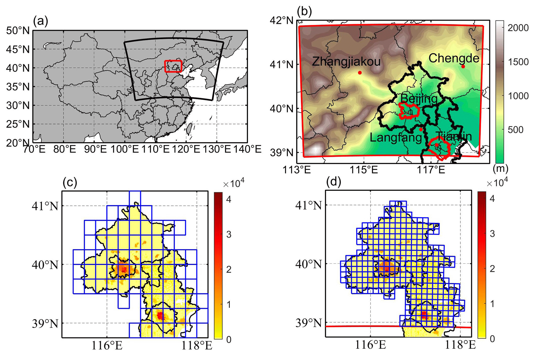
Figure 1 (a) The 10 km WRF domain (red box) nested inside a 30 km resolution WRF domain (large black sector). (b) The inner domain topography and major conurbations (red dots), with the urban areas of Beijing and Tianjin enclosed in red curves. Panels (c) and (d) show the population density (persons per km²) of Beijing and Tianjin provinces (defined by black borders) in 2010 and the grid cells within the Beijing–Tianjin province (blue boxes) when downscaled by ISIMIP (c) and WRF (d).

2 Data and methods

2.1 Scenarios, ESM, downscaling methods, and bias correction

The scenarios, ESM, downscaling methods, and bias-correction methods we use here are as described in detail by Wang et al. (2022), and we just summarize the method briefly here. We use three different scenarios: RCP4.5 and RCP8.5 (Riahi et al., 2011) as well as the GeoMIP G4 scenario, which span a useful range of climate scenarios. RCP4.5 is similar (Vandyck et al., 2016) to the expected trajectory of emissions under the 2015 Paris Climate Accord agreed nationally determined contributions (NDCs). RCP8.5 represents a formerly business-as-usual scenario with no climate mitigation policies and a large signal-to-noise ratio. G4 represents a similar radiative forcing as produced by the 1991 Mount Pinatubo volcanic eruption repeating every 4 years.

Climate simulations are performed by four ESMs: BNU-ESM (Ji et al., 2014), HadGEM2-ES (Collins et al., 2011), MIROC-ESM (Watanabe et al., 2011), and MIROC-ESM-CHEM (Watanabe et al., 2011). We compare dynamical and statistical downscaling methods to convert the ESM data to scales more suited to capturing differences between contrasting rural and urban environments. To validate the downscaled AP from model results, we use the daily temperature, humidity, and wind speed during 2008–2017 from the gridded observational dataset CN05.1 with the resolution of $\mathrm{0.25}{}^{\circ }\times {\mathrm{0.25}}^{\circ }$ based on the observational data from more than 2400 surface meteorological stations in China, which are interpolated using the “anomaly approach” (Wu and Gao, 2013). This dataset is widely used and has good performance relative to other reanalysis datasets over China (Zhou et al., 2016; Y. Yang et al., 2019, 2023; Yang and Tang, 2023). Dynamical downscaling for the four ESM datasets was done with WRFv.3.9.1 with a parameter set used for urban China studies (Wang et al., 2012) in two nested domains at 30 and 10 km resolution over two time slices (2008–2017 and 2060–2069). We corrected the biases in WRF output using the quantile delta mapping method (QDM; Wilcke et al., 2013) with ERA5 (Hersbach et al., 2018) to preserve the mean probability density function of the output over the domain without degrading the WRF spatial pattern. All WRF results presented are after QDM bias correction. Statistical downscaling was done with the trend-preserving statistical bias-correction Inter-Sectoral Impact Model Intercomparison Project (ISIMIP) method (Hempel et al., 2013) for the raw ESM output, producing output matching the mean ERA5 observational data in the reference historical period with the same spatial resolution, while allowing the individual ESM trends in each variable to be preserved.

2.2 PM_2.5 concentration and emission data

In China there were few PM_2.5 monitoring stations before 2013 (Xue et al., 2021). However, aerosol optical depths produced by the Moderate Resolution Imaging Spectroradiometer (MODIS) have been used to build a daily PM_2.5 concentration dataset (ChinaHighPM_2.5) at 1 km resolution from 2000 to 2018 (Wei et al., 2021). We use monthly PM_2.5 concentration data during 2008–2015 from ChinaHighPM_2.5 to train the MLR model and the data during 2016–2017 to validate it. Figure S1 in the Supplement shows the annual PM_2.5 concentration over Beijing areas during 2008 (a) and 2017 (b).

Recent gridded monthly PM_2.5 emission data were derived from the Hemispheric Transport of Air Pollution (HTAP_V3) with a resolution of ${\mathrm{0.1}}^{\circ }\times {\mathrm{0.1}}^{\circ }$ during 2008–2017, which is a widely used anthropogenic emission dataset (Janssens-Maenhout et al., 2015). PM_2.5 emissions over Beijing areas during 2008 (c) and 2017 (d) are shown in Fig. S1.

Future gridded monthly PM_2.5 emissions to 2050 are available in the ECLIPSE V6b database (Stohl et al., 2015), generated by the GAINS (Greenhouse gas Air pollution Interactions and Synergies) model (Klimont et al., 2017). The ECLIPSE V6b baseline emission scenario assumes that future anthropogenic emissions are consistent with those under current environmental policies; hence, it is the “worst” scenario without considering any mitigation measures (M. Li et al., 2018; Nguyen et al., 2020). Projected emissions are shown in Fig. S2, with emissions plateauing at ∼40 kt yr⁻¹ after 2030, so we assume that 2060s levels are similar. These ECLIPSE projections are significantly larger than present-day estimates from HTAP_V3. We therefore estimate 2060s emissions as the recent gridded monthly PM_2.5 emissions from HTAP_V3 scaled by the ratios of 2050 ECLIPSE emissions to average annual emissions between 2010 and 2015. Before processing data, PM_2.5 concentration is bilinearly interpolated to the WRF and ISIMIP grids, while PM_2.5 emissions are conservatively interpolated to the target grids.

2.3 Apparent temperature

We used a widely used empirical formula to calculate the apparent temperature under shade (Steadman, 1984) that combines various meteorological fields, which also has been widely used to study heat waves, heat stress, and temperature-related mortality (Perkins and Alexander, 2013; Lyon and Barnston, 2017; Lee and Sheridan, 2018; Zhu et al., 2021):

$$\begin{array}{}\text{(1)}& \text{AP}=-\mathrm{2.7}+\mathrm{1.04}\times T+\mathrm{2}\times P-\mathrm{0.65}\times W,\end{array}$$

where AP is the apparent temperature (^∘C) under shade, meaning that radiation is not considered; T is the 2 m temperature (^∘C), W is the wind speed at 10 m above the ground (m s⁻¹), and P is the vapor pressure (kPa) calculated by

$$\begin{array}{}\text{(2)}& P=P_{\text{s}}\times \text{RH},\end{array}$$

where P_s is the saturation vapor pressure (kPa), and RH is the relative humidity (%). P_s is calculated using the Tetens empirical formula (Murray, 1966).

$$\begin{array}{}\text{(3)}& P_{\text{s}}=\left\{\begin{array}{l}\mathrm{0.61078}\times e^{\left(\frac{\mathrm{17.2693882}\times T}{T+\mathrm{237.3}}\right),T\ge \mathrm{0}}\\ \mathrm{0.61078}\times e^{\left(\frac{\mathrm{21.8745584}\times \left(T-\mathrm{3}\right)}{T+\mathrm{265.5}}\right),T<\mathrm{0}}\end{array}\right.\end{array}$$

To assess the potential risks of heat-related exposure from apparent temperature, we also count the number of days with AP > 32 ^∘C (NdAP_32) in the Beijing–Tianjin province. This threshold does not lead to extreme risk and death; instead, it is classified as requiring “extreme caution” by the US National Weather Service (National Weather Service Weather Forecast Office, https://www.weather.gov/ama/heatindex, last access: 14 September 2023) but carries risks of heatstroke, cramps, and exhaustion (Table S1 in the Supplement). A threshold of 39 ^∘C is classified as “dangerous” with a risk of heatstroke. While hotter AP thresholds would give a more direct estimate of health risks, the statistics of these presently rare events mean that detecting differences between scenarios is less reliable than using the cooler NdAP_32 threshold simply because the likelihood of rare events is more difficult to accurately quantify than more common events that are sampled more frequently. There is evidence that in some distributions, the likelihood of extremes will increase more rapidly than central parts of a probability distribution: for example, large Atlantic hurricanes increasing faster than smaller ones (Grinsted et al., 2013). But the conservative assumption is that similar differences between scenarios would apply for higher thresholds as well as lower ones.

2.4 Population dataset

Since health impacts scale with the number of people affected, we calculate the NdAP_32 weighted by population (Fig. 1c and d). We employ gridded population data (Fu et al., 2014; https://doi.org/10.3974/geodb.2014.01.06.V1) with a spatial resolution of 1×1 km collected in 2010. The population density distribution in Beijing and Tianjin provinces with the ISIMIP and WRF grid cells contained is shown in Fig. 1c and d.

2.5 MLR model calibration

Many meteorological factors, such as temperature (You et al., 2017), precipitation (Guo et al., 2016), wind speed (Yin et al., 2017), radiation (Chen et al., 2017), and planetary boundary layer height (Zheng et al., 2017), can affect the PM_2.5 concentration. Their relative importance differs regionally. But here we consider only differences that are produced by the three scenarios, so, for example, we do not include precipitation in our analysis because none of the ESMs simulate significant changes in our domain (Table S2). Previous studies have shown that wind and humidity are the dominant meteorological variables for PM_2.5 concentration in the region we study (Chen et al., 2020), while changes in temperature and winds obviously impact local concentrations. Hence, we generate an MLR model between PM_2.5 and temperature (T), relative humidity (H), zonal wind (U), meridional wind (V), and PM_2.5 emissions (E) at every grid cell as follows:

$$\begin{array}{}\text{(4)}& {\mathrm{PM}}_{\mathrm{2.5}}=\sum a_i{X}_i+b,\end{array}$$

where $X_{i(i=\mathrm{1},\mathrm{2},\mathrm{3},\mathrm{4},\mathrm{5})}$ represents the five factors, a_i represents the regression coefficients of X_i with PM_2.5, and b is the intercept, which is a constant. We assume that all factors should be included in the regression. All the meteorological variables are from the statistical and dynamical downscaling and bias-corrected results during 2008–2017, with the first 8 years used for training the model and the second 2 years used for validating the model. We train the MLR for the four ESMs under statistical and dynamical downscaling in each grid cell separately, thus accounting for spatial differences in the weighting of X_i across the domain. Meteorological variables under G4, RCP4.5, and RCP8.5 during 2060–2069 are used for projection.

Here, we use PM_2.5 concentration including both primary and secondary PM_2.5 as the dependent variable and primary PM_2.5 emissions and meteorological factors as independent variables in the MLR. Future PM_2.5 emissions will change in ways that are rather speculative as they depend on technological innovation and policies that are inherently unpredictable. The MLR assumes that the past emissions mix and secondary aerosols remain unchanged in the future, but meteorological factors will also indirectly impact secondary PM_2.5 to some extent.

The contributions of meteorology and PM_2.5 emissions to future concentrations are examined by using recent PM_2.5 emissions (baseline) and future PM_2.5 emissions (mitigation), as well as the downscaled climate scenarios. Modeled PM_2.5 concentration using recent meteorology and PM_2.5 emissions during 2008–2017 (2010s) is considered to be our reference.

Collinearity of variables is inevitable in our domain. The domination of the seasonal winter and summer monsoonal weather patterns means that temperatures, precipitation, and wind direction are all highly seasonal and correlated. In winter, precipitation is minimal and northerly winds predominate, and in summer the opposite is true. These three meteorological fields are important and also important for emissions, since sources are essentially absent from the north, while temperature and humidity dominate aerosol microphysics.

We use the variance inflation factor (VIF) to test if there is excessive collinearity in our MLR models. Generally, if the VIF value is greater than 10, there is a collinearity problem between variables. Figure S3 shows that there are indeed collinearity problems in some areas, but not in the Beijing–Tianjin province, so there is no impact on the results for the urban areas. We explored the impact of collinearity on the results in high-VIF grid cells by removing factors with VIF greater than 10 and the full variable model (Figs. S4 and S5). Using ISIMIP downscaling, we only removed the temperature, while we removed the temperature and U wind in the WRF method. Changes in PM_2.5 concentration range from −1 to 1 µg m⁻³ in all ESMs under G4 with the baseline scenario (Fig. S4). In contrast, PM_2.5 concentrations decreased by 5–15 µg m⁻³ with the “mitigation” scenario (Fig. S5) after dealing with the collinearity problem. This means that PM_2.5 concentration has more sensitivity to the PM_2.5 emission after accounting for collinearity. Although the absolute PM_2.5 concentrations are different accounting for collinearity, there are no significant differences in the changes in PM_2.5 concentration between G4 and the 2010s, RCP4.5, and RCP8.5 in the Beijing–Tianjin province.

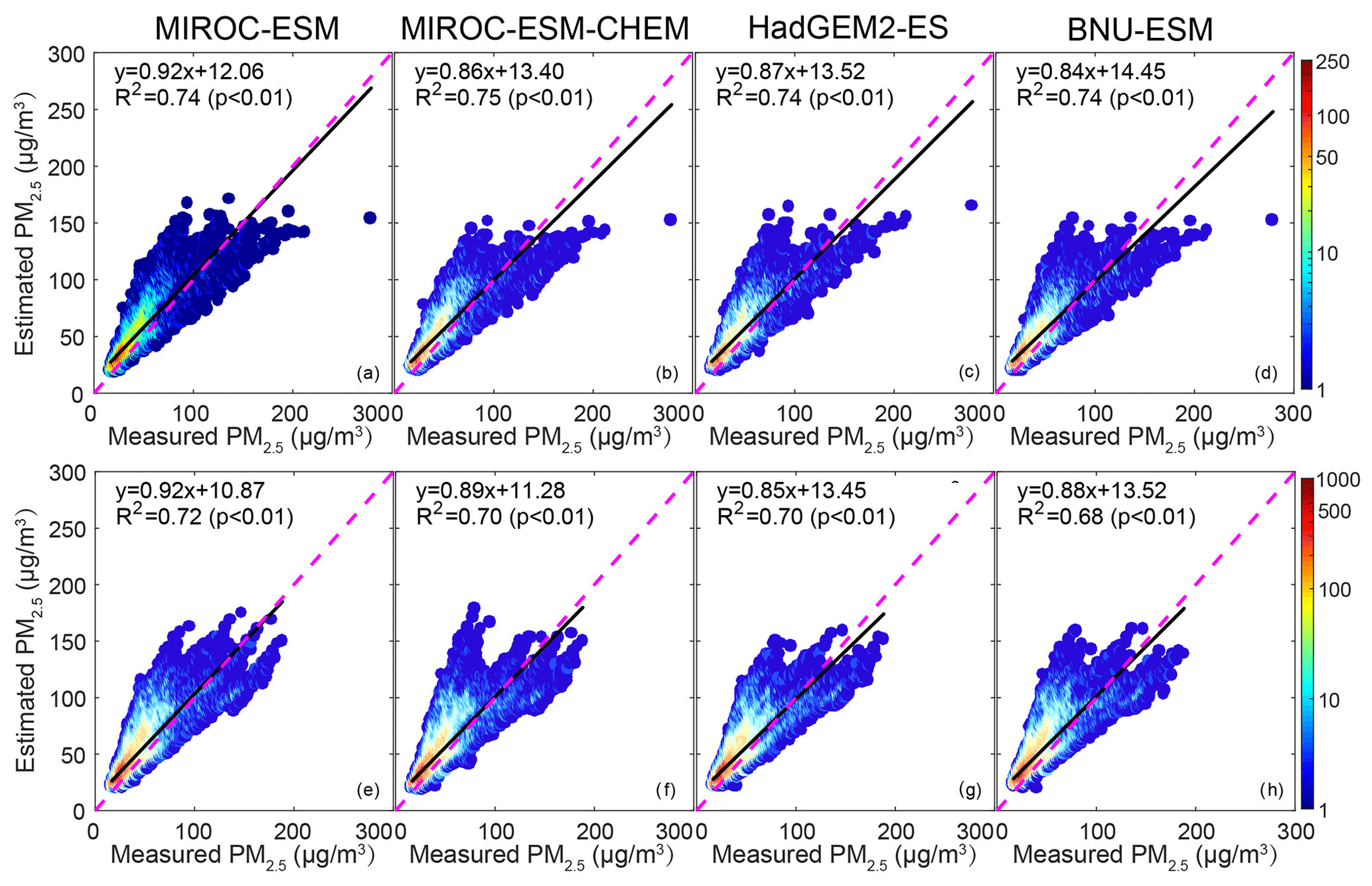
Figure 2 Scattergrams of PM_2.5 concentration derived by MODIS and estimated by MLR during the validation period (2016–2017). Top panels (a–d) are the ISIMIP statistical downscaling results, and bottom panels (e–h) are the WRF dynamical downscaling results. R² means the variance explained by the MLR, and the color bar denotes the density of data points at integer intervals.

2.6 MLR model validation

Figure 2 shows the scattergram of PM_2.5 concentration between the ChinaHighPM_2.5 dataset and MLR model during the validation period based on ISIMIP and WRF results. Observations and MLR models have Pearson's correlations coefficients around 0.86 for ISIMIP results during the validation period, and the coefficient of determination of MLRs is 0.74–0.75 (Fig. 2a–d). WRF Pearson's correlations are slightly lower at 0.82–0.85, and explained variance ranges from 0.68–0.72 (Fig. 2e–h). These results are similar to those found by Jin et al. (2022). We also compare the spatial patterns of observed and modeled PM_2.5 in Fig. S6. Both ISIMIP and WRF results can simulate the distribution characteristics of high concentrations of PM_2.5 in the southeast and low concentrations in the northwest.

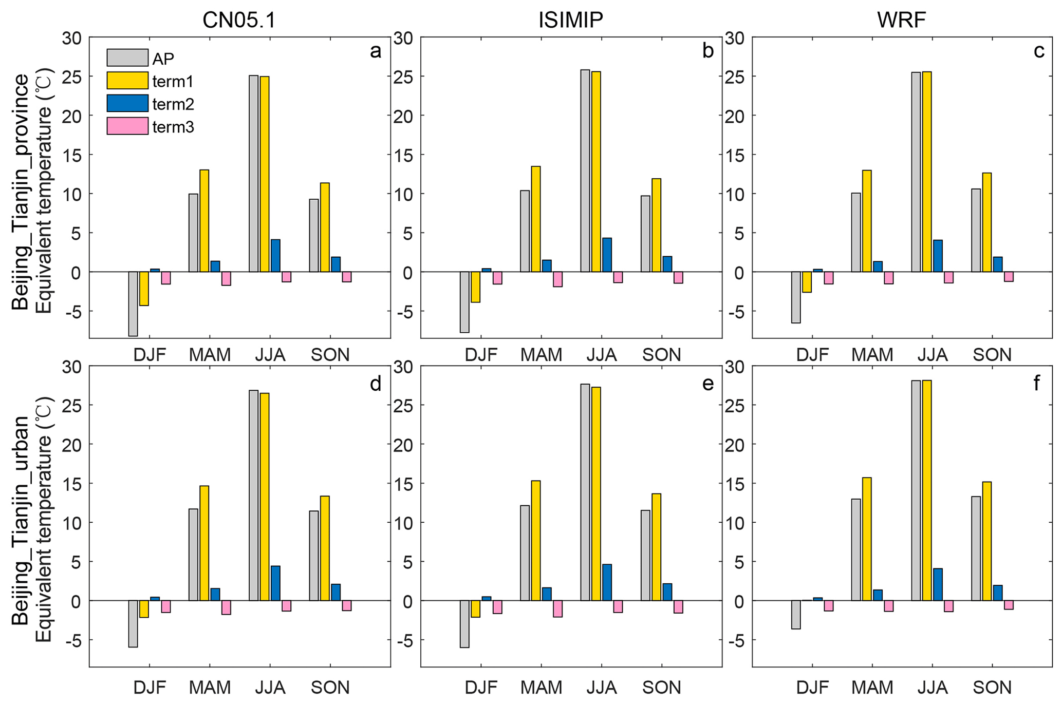
Figure 3 Seasonally averaged AP and equivalent temperature of each term in Eq. (1) for the Beijing–Tianjin province (a–c) and Beijing–Tianjin urban areas (d–f) during 2008–2017 from CN05.1 (a, d), the four-model ensemble mean after ISIMIP (b, e), and the ensemble mean after WRF (c, f). Term 1 is 1.04 T, term 2 is 2 P, and term 3 is −0.65 W.

We also tested the accuracy of our MLR model projection against simulations (Li et al., 2023) with the Community Multiscale Air Quality (CMAQ) model developed by the United States Environmental Protection Agency, which can simulate particulate matter on local scales (Foley et al., 2010; X. Yang et al., 2019) when coupled to WRF. We used the same meteorological forcing as Li et al. (2023) with the EIT1 PM_2.5 emissions scenario in 2050 under RCP4.5 (Fig. S7). The spatial patterns are well correlated in all seasons (0.68–0.73), but PM_2.5 concentrations are about twice as high in our MLR model as those from Li et al. (2023). PM_2.5 concentrations from our regression model are also higher than in the referenced data during 2008–2017. While the differences in absolute PM_2.5 concentrations are significant, we mainly consider differences in the PM_2.5 concentration between G4 and two RCPs (RCP4.5 and RCP8.5) in our study, which we cannot compare with the single RCP4.5 scenario simulated by Li et al. (2023). We do compare the spatial pattern of differences in PM_2.5 concentration between the baseline and EIT1 under RCP4.5. Because of the small slope coefficient of PM_2.5 emissions in our MLR, we do not capture the large reduction of the PM_2.5 concentration in the Beijing city center seen by Li et al. (2023) (Fig. S8).

2.7 Relative risks of mortality related to PM_2.5

We estimate the effects of PM_2.5 on mortality by considering changes in the relative risk (RR) of mortality related to PM_2.5. We lack data on mortality rates in the study domain, without which we cannot estimate numbers of fatalities, just the average population-weighted RR. Burnett et al. (2014) established the integrated exposure–response functions we use. The RR is nonlinear in concentration – that is, an initially low-PM_2.5 region will suffer higher mortality and RR than an initially high-PM_2.5 region if PM_2.5 is increased by the same amount. Ran et al. (2023) provide RR values for PM_2.5 concentrations up to 200 µg m⁻³ that include the five main major disease end points (Global Burden of Disease Collaborative Network, 2013) of PM_2.5-related mortality: chronic obstructive pulmonary disease, ischemic heart disease, lung cancer, lung respiratory infection, and stroke. We calculate the average population-weighted relative risks based on the gridded population dataset (Sect. 2.4) and PM_2.5 concentration in the Beijing–Tianjin province defined in Fig. 1c–d, following Ran et al. (2023).

$$\begin{array}{}\text{(5)}& {\mathrm{RR}}_{\text{pop},k}={\displaystyle \frac{{\sum }_{g=\mathrm{1}}^G{\mathrm{POP}}_g\times {\mathrm{RR}}_k\left(C_g\right)}{{\sum }_{g=\mathrm{1}}^G{\text{POP}}_g}}\end{array}$$

RR_pop,k is the average population-weighted relative risk of disease k (k=1–5), POP_g is the population of grid g, and RR_k (C_g) is the relative risk of disease k when the PM_2.5 concentration is C_g in the grid of g.

2.8 Determination of contributions to changes in AP and PM_2.5

Equation (1) describes how AP is calculated, and this can be broken down into how much equivalent temperature is produced by each term (Fig. 3), with 2008–2017 as the baseline interval for season-by-season contributors to AP. Cross-scenario seasonal differences in contributors are then calculated as follows. We use an MLR approach, since this minimizes the square differences from the mean across the dataset, with the attendant assumption of independence between the data. Alternatives may also be considered that, e.g., minimize the impact of outliers by considering the magnitude of the differences, but we prefer to keep the attractive properties of a least-squares approach. The dependent variable in the MLR is the change in AP (Δ AP), and the independent variables are changes in each factor for each future scenario,

$$\begin{array}{}\text{(6)}& \mathrm{\Delta }\text{AP}=\sum {\mathit{\alpha }}_i{X}_i+\mathit{\beta },\end{array}$$

where $X_{i(i=\mathrm{1},\mathrm{2},\mathrm{3})}$ represents the daily changes in the three meteorological factors between two scenarios for 2 m temperature (ΔT), 2 m relative humidity (Δ RH), and 10 m wind speed (ΔW); α_i represents the regression coefficients of X_i with Δ AP; and β is the intercept, which is a constant. We assume that all three meteorological factors should be included in the regression, and we estimate the contributions of each factor to changes in AP as

$$\begin{array}{}\text{(7)}& K_i={\displaystyle \frac{{\mathit{\alpha }}_i\stackrel{\mathrm{‾}}{X_i}}{\sum {\mathit{\alpha }}_i\overline{X_i}}},\end{array}$$

where $K_{i(i=\mathrm{1},\mathrm{2},\mathrm{3})}$ represents the contributions (in units of temperature) from each factor to the changes in the AP, and $\stackrel{\mathrm{‾}}{X_i}$ represents the mean differences in temperature equivalent due to each factor between two scenarios.

The contribution of changes to each factor in changes in PM_2.5 is simpler since we assume that the relationship between each factor and PM_2.5 is linear, and so its contribution is the ratio of the product of the regression coefficient and the change in each factor to the change in PM_2.5.

3 Results

3.1 Recent apparent temperatures

Figure 3 shows the seasonally averaged AP and equivalent temperatures caused by temperature, relative humidity, and wind speed in the Beijing–Tianjin province and Beijing–Tianjin urban areas during 2008–2017. According to the CN05.1 results (Fig. 3a, d), AP and the three separate terms show similar seasonal patterns over the whole province and just the urban areas. Vapor pressure is higher in summer and wind speed is higher in spring. AP is lower than 2 m temperature in all seasons except summer and especially lower in winter. AP, temperature, vapor pressure, and wind speed are all higher in urban areas than in the surrounding rural region in any season. The ISIMIP results (Fig. 3b, e), by design, perfectly reproduce the CN05.1 seasonal characteristics of AP, temperature, vapor pressure, and wind speed. WRF shows a similar pattern as that from CN05.1, but for the Beijing–Tianjin province, WRF overestimates both 2 m temperature and AP in winter by 2.1 ^∘C and by 1.7 ^∘C, respectively, relative to CN05.1 (Fig. 3c). In the Beijing–Tianjin urban areas, WRF overestimates the temperature and AP relative to CN05.1 in all seasons, especially in winter (Fig. 3f).

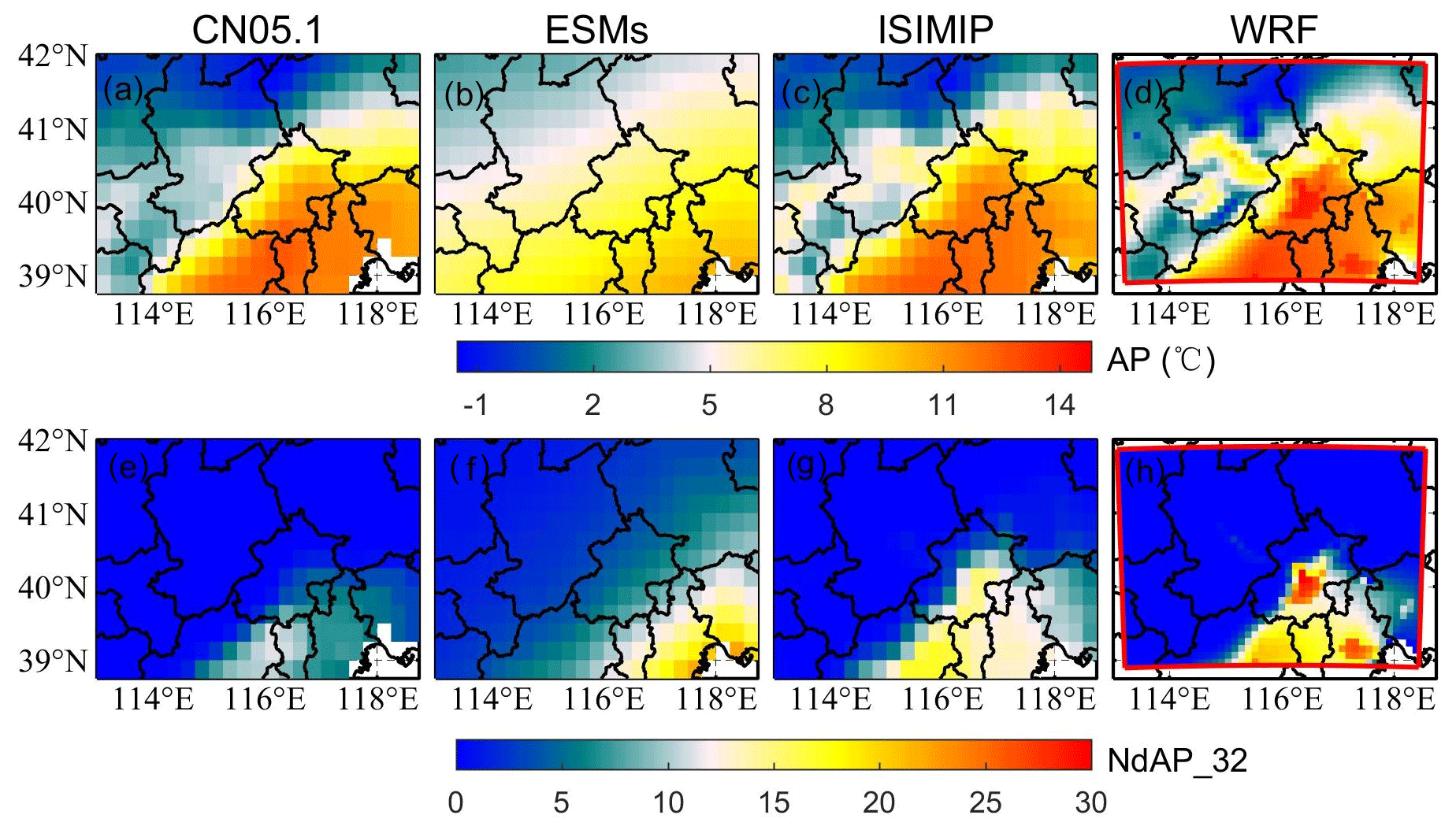
Figure 4 Top row: the spatial distribution of mean apparent temperature from CN05.1 (a), raw ESM ensemble mean after bilinear interpolation (b), four-model ensemble mean after ISIMIP (c), and ensemble mean after WRF (d) during 2008–2017. Bottom row: the spatial distribution of the annual mean number of days with AP > 32 ^∘C from CN05.1 (e), ESMs (f), ISIMIP (e), and WRF (f) during 2008–2017. Figures S9 and S10 show the pattern of AP and NdAP_32 for the individual ESMs.

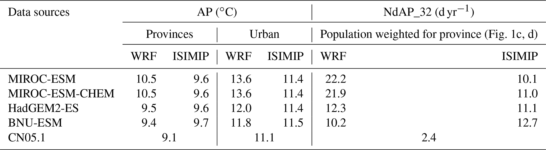
We compare the simulations of mean apparent temperature and NdAP_32 from both WRF dynamical downscaling with QDM and from ISIMIP statistical downscaling during 2008–2017 in Fig. 4. Both the WRF with QDM and ISIMIP methods produce a pattern of apparent temperature which is close to that from CN05.1. While the raw AP from ESMs is overestimated in the high mountains in Zhangjiakou and underestimated on the southern plain, it shares a similar pattern with temperature from ESMs (Wang et al., 2022). The raw ESM outputs were improved after dynamical and statistical downscaling. The average annual AP from ISIMIP (9.6–9.7 ^∘C) is 0.5 ^∘C higher than that from CN05.1 (9.1 ^∘C) over the Beijing–Tianjin province for all ESMs (Table 1). WRF produces warmer apparent temperatures in the city centers of Beijing and Tianjin and lower ones in the high Zhangjiakou mountains than recorded in the lower-resolution CN05.1 observations. There are also differences between different models after WRF downscaling. For example, apparent temperatures from the two MIROC models downscaled by WRF are the warmest. In contrast, AP from all four ESMs after ISIMIP shows very similar patterns (Fig. S9).

ESMs tend to overestimate the number of days with AP > 32 ^∘C in southeastern Beijing and the whole Tianjin province. Both ISIMIP and WRF appear to overestimate the NdAP_32 in Beijing urban areas and the southerly lowland areas, although NdAP_32 is close to zero in the colder rural areas at relatively high altitude for both downscaling methods. Some of these differences may be due to the WRF simulations being at a finer resolution than the ${\mathrm{0.25}}^{\circ }\times \mathrm{0.25}$ ^∘C N05.1, leading to higher probabilities of high AP in urban areas (Fig. 5d). ISIMIP results also show slight overestimations, especially in the tails of the distribution (AP > 30 ^∘C) for urban areas (Fig. 5c). CN05.1 gives about 5 NdAP_32 days per year in southern Beijing and Tianjin, but there are nearly 15 NdAP_32 days from ISIMIP and over 20 NdAP_32 days per year from WRF downscaling in Beijing–Tianjin urban areas during 2008–2017. NdAP_32 from WRF and ISIMIP downscaling of all ESMs is overestimated relative to CN05.1. But there are differences in ESMs under the two downscalings: with ISIMIP, HadGEM2-ES and BNU-ESM have more NdAP_32 days than the two MIROC models, while the reverse occurs with WRF (Fig. S10).

Table 1 The annual mean apparent temperature and population-weighted NdAP_32 in the Beijing–Tianjin province and Beijing–Tianjin urban areas (Fig. 1b) from CN05.1, ISIMIP, and WRF during 2008–2017.

The Taylor diagram of the daily mean apparent temperature in the Beijing–Tianjin province and Beijing–Tianjin urban areas from 2008–2017 for the four ESMs shows that correlation coefficients between ESMs and CN05.1 are greater than 0.85 under both downscaling methods. Although there are differences between ESMs, the performance of WRF, with a higher correlation coefficient and smaller SD (standard deviation) and RMSD (root mean square deviation), is usually superior to ISIMIP (Fig. S11). Taking the Beijing–Tianjin urban areas as an example (Fig. S11b), under the ISIMIP method, MIROC-ESM, MIROC-ESM-CHEM, and HadGEM2-ES have the same correlation coefficient (0.92) and RMSD (5.4 ^∘C) as the CN05.1, while BNU-ESM has a lower correlation coefficient (0.88) and higher RMSD (7.0 ^∘C). Under WRF simulations, MIROC-ESM and MIROC-ESM-CHEM have larger correlation coefficients and smaller RMSD with CN05.1 than HadGEM2-ES and BNU-ESM.

Figure 5 shows the probability density functions (PDFs) of daily AP from the four ESMs under ISIMIP and WRF in the Beijing–Tianjin province and Beijing–Tianjin urban areas during 2008–2017. ISIMIP overestimates the probability of extremely cold AP relative to CN05.1 (especially BNU-ESM), although all ESMs reproduce the CN05.1 PDF well at high AP. WRF can reproduce the CN05.1 distribution of AP better than ISIMIP, but high AP is overestimated relative to CN05.1 and the urban areas perform less well than the whole Beijing–Tianjin province. In urban areas all ESMs driving WRF tend to underestimate the probability of lower AP and to overestimate the probability of higher AP, especially the two MIROC models (Fig. 5d). Figure S12 displays the annual cycle of monthly AP, with ISIMIP proving to be excellent by design at reproducing the monthly AP. Under WRF downscaling AP shows more across-model differences, especially during summer, and with greater spread for the urban areas.

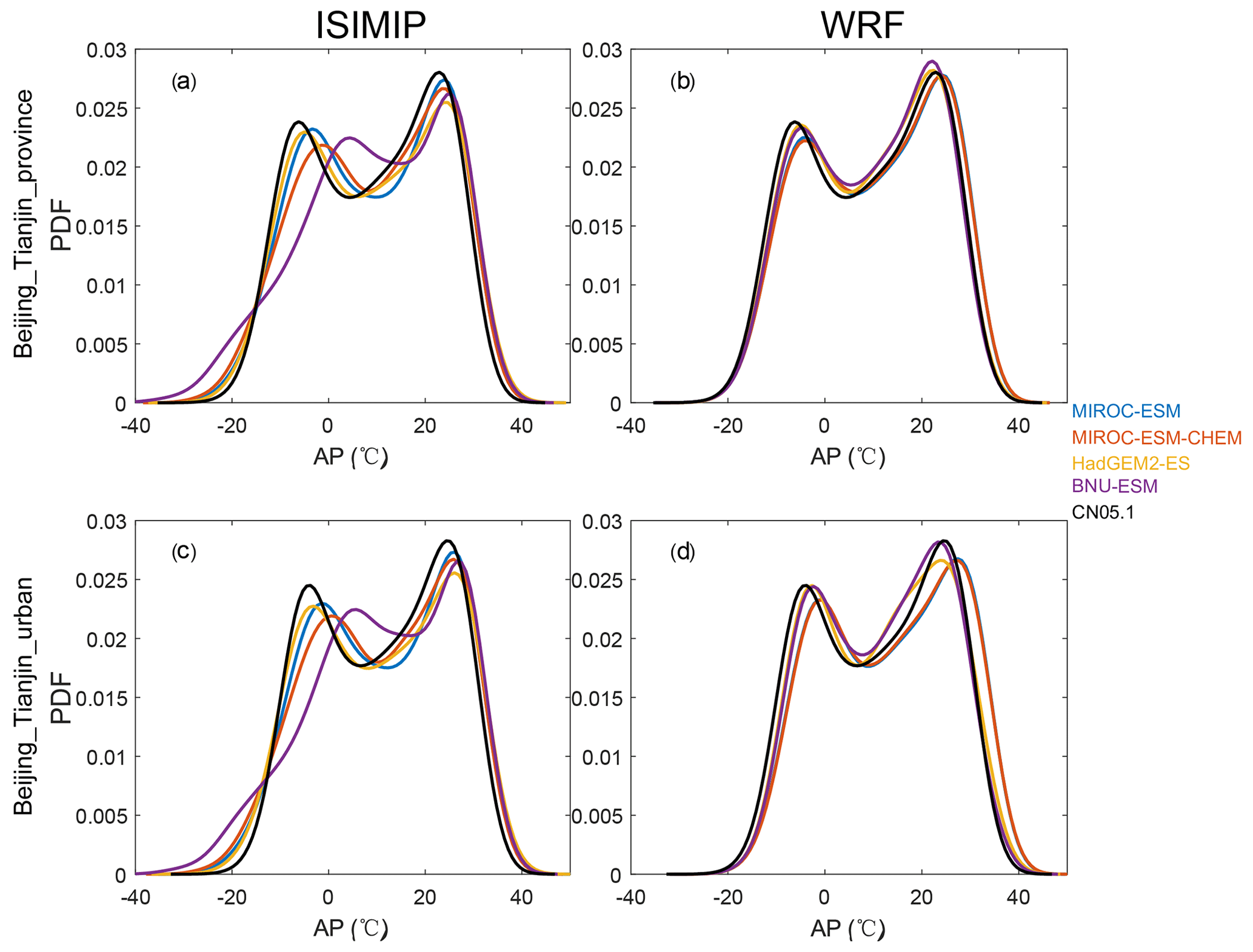
Figure 5 The probability density function (PDF) for daily apparent temperature under ISIMIP (a, c) and WRF (b, d) results in the Beijing–Tianjin province (a, b) and Beijing–Tianjin urban areas (c, d) during 2008–2017.

3.2 2060s apparent temperatures

3.2.1 Changes in apparent temperature

Figure 6 shows the ISIMIP and WRF ensemble mean changes in the annual mean AP under G4 during 2060–2069 relative to the past and the two future RCP scenarios. ISIMIP-downscaled AP (Fig. 6a–c) shows significant anomalies (p<0.05), with whole-domain rises of 2.0 ^∘C in G4–2010s and decreases of 1.0 and 2.8 ^∘C in G4–RCP4.5 and G4–RCP8.5, respectively. In WRF results, AP under G4 is about 1–2 ^∘C warmer than that under the 2010s, as well as 0.8 and 2.5 ^∘C colder than that under RCP4.5 and RCP8.5 over the whole domain. Individual ESM results downscaled by ISIMIP and WRF are in Figs. S14 and S15. For both ISIMIP and WRF downscaling results, the two MIROC models show stronger warming than the other two models between G4 and the 2010s. WRF-downscaled AP driven by HadGEM2-ES exhibits the strongest cooling, with decreases of 1.7 ^∘C between G4 and RCP4.5 and decreases of 3.0 ^∘C between G4 and RCP8.5. Although different ESMs show different changes in AP between G4 and other scenarios, changes in AP are almost the same everywhere for a given ESM in the ISIMIP results (Fig. S14). WRF-downscaled AP anomalies driven by two MIROC models are larger in the Zhangjiakou mountains and smaller in the Beijing urban areas and Tianjin between G4 and the 2010s (Fig. S15). Changes in AP from ISIMIP results, whether across whole province or just the urban areas, are statistically identical given scenarios (Table 2), which is consistent with patterns in Fig. 6. AP under G4 is 0.8 ^∘C (1.0 ^∘C) and 2.6 ^∘C (2.8 ^∘C) colder than that under RCP4.5 and RCP8.5 in Beijing–Tianjin urban areas from ISIMIP (WRF) results. The warming between G4 and the 2010s in urban areas is 1.0 ^∘C in WRF results, while it is 2.0 ^∘C in ISIMIP results (Table 2).

Table 2 Difference in apparent temperature between the G4 and other scenarios for the Beijing–Tianjin province and Beijing–Tianjin urban areas as defined in Fig. 1b during 2060–2069. Bold indicates that the differences or changes are significant at the 5 % level according to the Wilcoxon signed rank test (units: ^∘C).

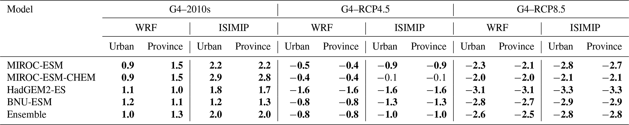
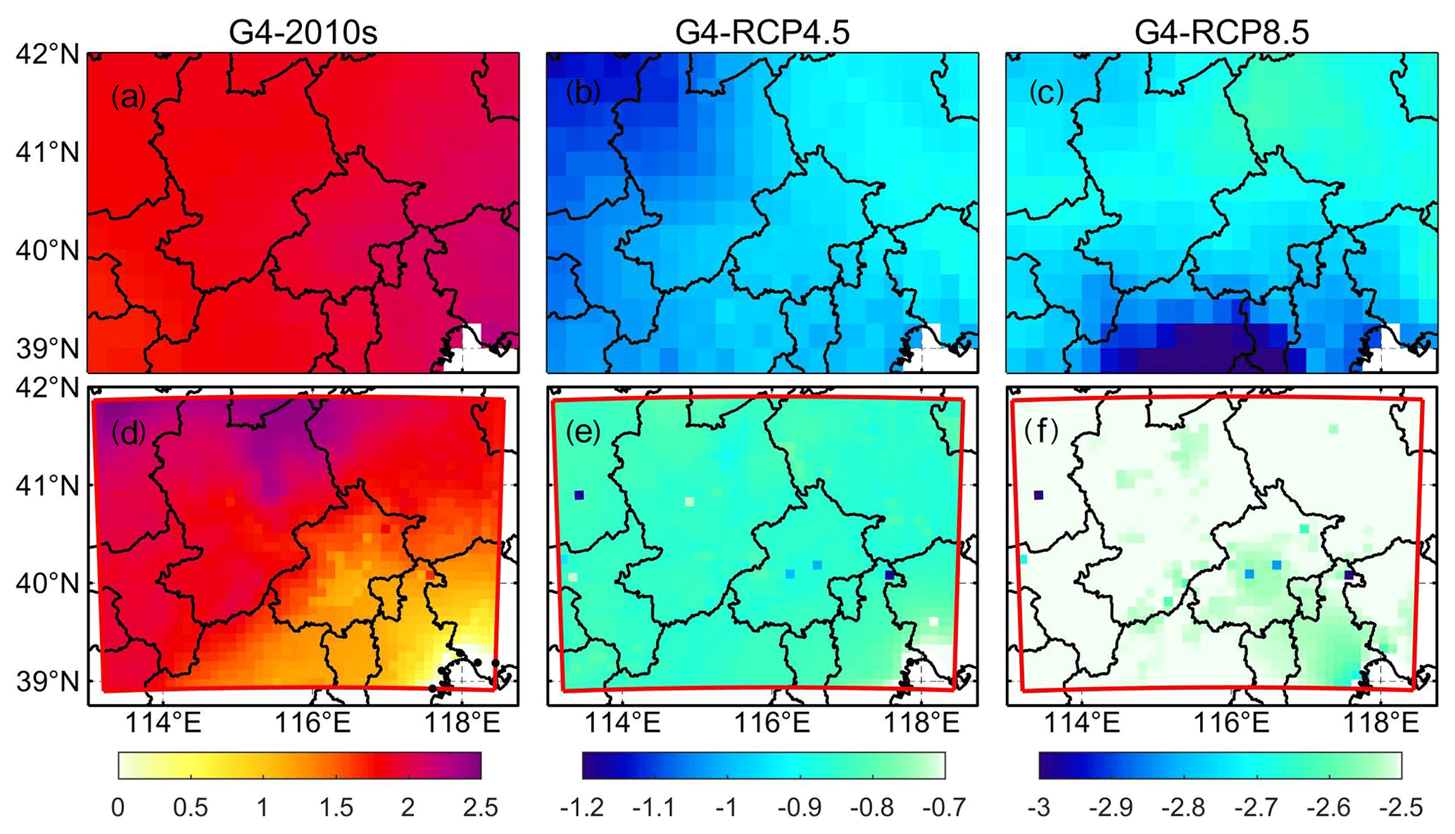
Figure 6 Spatial pattern of ensemble mean apparent temperature difference (^∘C) under different scenarios over 2060–2069: G4–2010s (a, d), G4–RCP4.5, (b, e), and G4–RCP8.5 (c, f) based on ISIMIP and WRF methods. The 2010s refer to the 2008–2017 period. Stippling indicates grid points where differences or changes are not significant at the 5 % level according to the Wilcoxon signed rank test.

3.2.2 Contributing factors to changes in AP

Figure 7 shows the ISIMIP and WRF ensemble mean changes in the annual mean AP anomalies for G4 during 2060–2069 relative to the past and the two future RCP scenarios. ISIMIP-downscaled AP (Fig. 7a–c) shows significant anomalies (p<0.05) across the whole domain, even for the relatively small differences in G4–RCP4.5. ΔAP by WRF is lower than that by ISIMIP. Between G4 and the 2010s, APs are projected to have increases of 1.8 (1.6), 2.1 (1.8), 2.4 (−0.2), and 1.8 (0.8) ^∘C from winter to autumn in ISIMIP (WRF) results. In ISIMIP results, the contribution of temperature ranges from 91 %–104 %, and the contribution of wind speed ranges from 3 %–10 % in all seasons, while the contribution of humidity is negative or insignificant (Fig. 7a). However, the contribution of humidity is positive in WRF results (Fig. 7a). Between RCP4.5 and the 2010s, annual mean AP is projected to increase by 3.0 and 1.8 ^∘C in ISIMIP and WRF results, respectively, which is higher than that between G4 and the 2010s. The increase in temperature and decrease in wind speed have a significant impact on the annual average ΔAP that contributed 97 % (94 %) and 4 % (3 %) to ISIMIP (WRF) results. The contributions of changes in humidity are significantly positive under G4 and RCP4.5 in WRF results, while it is the opposite in the ISIMIP results (Fig. 7a–b).

Relative to RCP4.5 in the 2060s, AP is projected to decrease by 1.0 (0.4), 0.7 (0.8), 0.8 (0.7), and 1.3 (1.4) ^∘C from winter to autumn under G4 in ISIMIP (WRF) results (Fig. 7c). In summer, the contributions from changes in temperature and humidity are 94 % (105 %) and 8 % (−9 %) in ISIMIP (WRF) results. There are insignificant contributions from wind speed under ISIMIP results but a significant slight positive contribution (0.7 %–4 %) under WRF results (Fig. 7c). The annual mean AP under G4 is 2.8 (2.6) ^∘C lower than that under RCP8.5 in the ISIMIP (WRF) result. In this case, the contribution of changes in wind to ΔAP ranges from 3 %–5 % by ISIMIP, while it is close to 0 by WRF. As expected, ΔAP is mainly determined by the changes in temperature, with contributions usually above 90 % between different scenarios.

A useful measure of heat impacts that may be missed if considering only air temperatures is the seasonality of the differences between AP and air temperature (Δ(AP–T); Fig. 8). The four-model ensemble annual mean Δ(AP–T) under ISIMIP is projected to rise by 0.4, 0.5, and 0.9 ^∘C under G4, RCP4.5, and RCP8.5 relative to the 2010s. Under WRF, Δ(AP–T) is much smaller than under ISIMIP but still rising faster than air temperatures: by 0.2, 0.3, and 0.5 ^∘C under G4, RCP4.5, and RCP8.5 relative to the 2010s, respectively. In general, the largest anomalies in Δ(AP–T) are in summer under both WRF and ISIMIP downscaling, but the two MIROC models under WRF have small or even negative Δ(AP–T) in summer with WRF.

3.2.3 Changes in the number of days with AP > 32 ^∘C

The NdAP_32 anomalies in Fig. 9 show that ISIMIP projects an increase of about 20 d yr⁻¹ with AP > 32 ^∘C for the southeast of the Beijing province and 10 d in the western areas of Beijing under G4 relative to the 2010s. NdAP_32 is about 10 d fewer under G4 than RCP4.5 with no clear spatial differences. G4 has about 35 fewer NdAP_32 days in the southern part of the domain and 20 fewer days in the western domain than the RCP8.5 scenario. In contrast, WRF suggests that most areas do not show any significant difference between G4 and the 2010s; while the anomalies relative to RCP4.5 are similar to ISIMIP, the differences are insignificant over more area than ISIMIP. G4–RCP8.5 anomalies with WRF are smaller than with ISIMIP, and differences are not significant in the high Zhangjiakou mountains. The urban areas show larger decreases in NdAP_32 than the more rural areas, even on the low-altitude plain. Individual ESMs show almost no statistically significant differences between G4 and RCP4.5 (Figs. S16 and S17), but the differences seen in Fig. 9 are significant because of the larger sample size in the significance test. All ESMs with ISIMIP show more NdAP_32 days in the urban areas under G4 than the 2010s, while the two MIROC models driving WRF show fewer NdAP_32 days in Beijing–Tianjin urban areas (Figs. S16, S17).

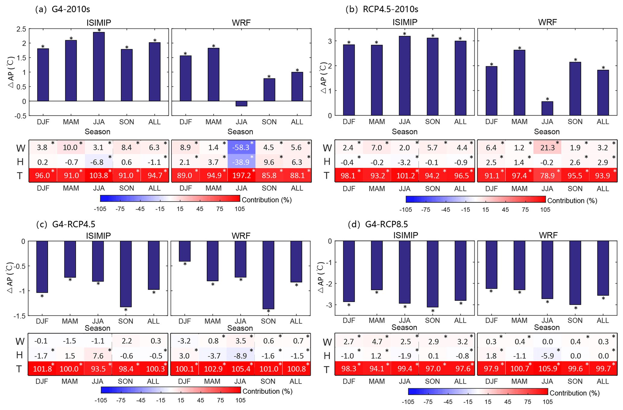
Figure 7 The seasonal changes in AP (ΔAP) and the seasonal contribution of climatic factors to ΔAP for Beijing and Tianjin urban areas under ISIMIP and WRF between G4 and the 2010s (a), RCP4.5 and the 2010s (b), G4 and RCP4.5, (c) and G4 and RCP8.5 (d) in the 2060s based on ensemble mean results. Colors and numbers in each cell correspond to the color bar, and the asterisks (*) above the columns and in the cells indicate that differences are significant at the 5 % significance level under the Wilcoxon test.

The PDF of daily apparent temperature in summer over Beijing–Tianjin urban areas (Fig. 10) shifts rightwards for G4, RCP4.5, and RCP8.5 during the 2060s relative to the 2010s. Figure 10 shows that by the 2060s, the dangerous threshold of AP > 39 ^∘C is crossed frequently under RCP8.5 with both WRF and ISIMIP downscaling, but for the RCP4.5 and G4 scenarios these events are much rarer. ISIMIP results tend to show higher probability tails (extreme events) than under WRF simulations.

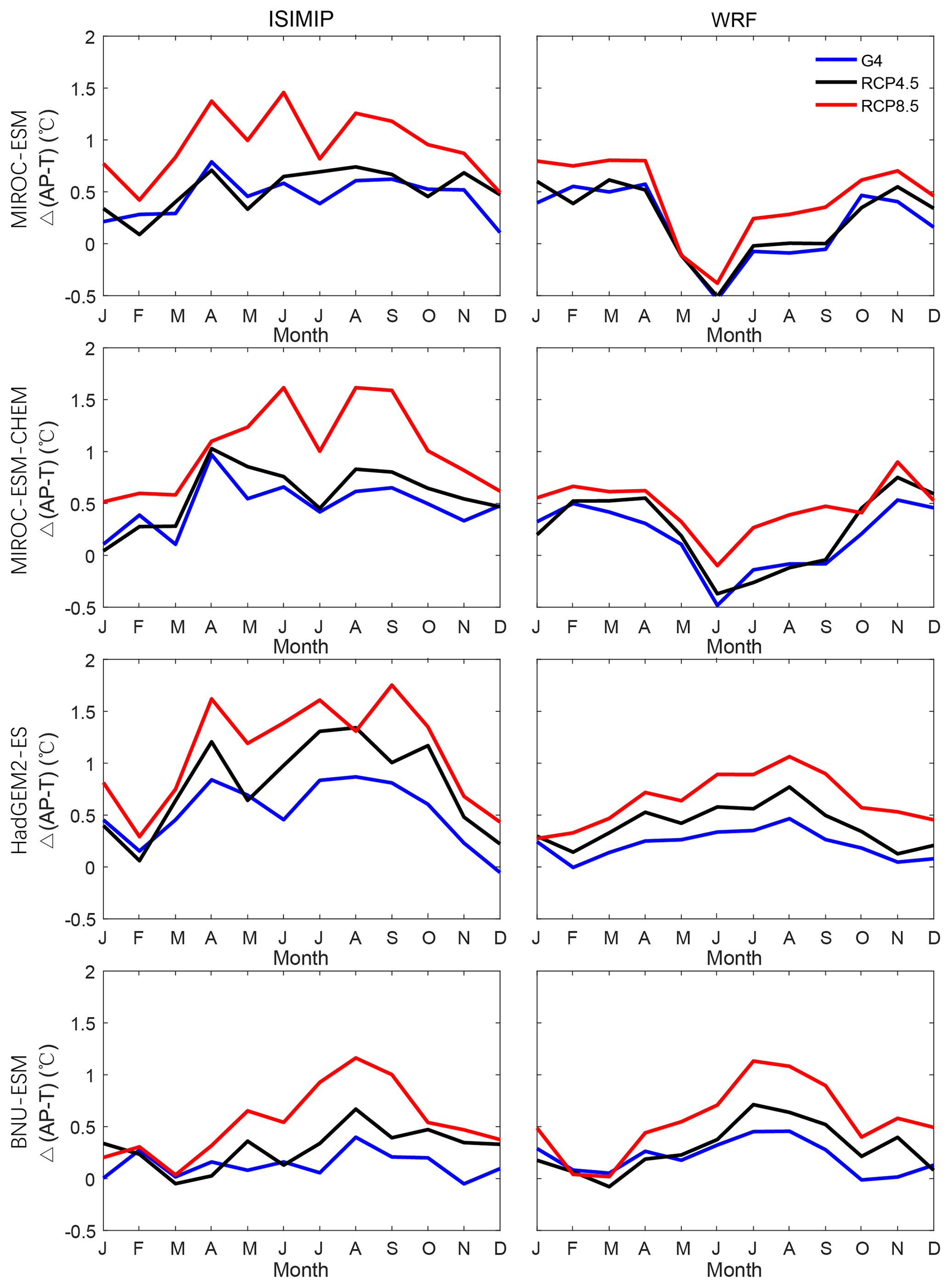
Figure 8 The change in apparent temperature based on air temperature under three scenarios (G4, RCP4.5, and RCP8.5) in four ESMs under ISIMIP (left column) and WRF (right column) for urban areas relative to the 2010s.

Population-weighted NdAP_32 in the 2060s for the Beijing–Tianjin province is shown in Table 3. ISIMIP downscaling suggests ensemble mean rises in NdAP_32 of 22.4 d yr⁻¹ under G4 relative to the 2010s but that G4 has 8.6 and 33.5 d yr⁻¹ less than RCP4.5 and RCP8.5, respectively. NdAP_32 from WRF under G4 is reduced by 19.6 d yr⁻¹ relative to RCP8.5 and by 6.3 d yr⁻¹ relative to RCP4.5 (Table 3).

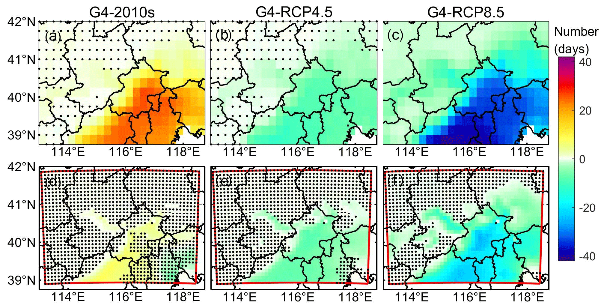
Figure 9 Ensemble mean differences in the annual number of days with AP > 32 ^∘C (NdAP_32) between scenarios for 2060–2069: G4–2010s (a, d), G4–RCP4.5, (b, e), and G4–RCP8.5 (c, f) based on the ISIMIP method and WRF. The 2010s mean the results simulated during 2008–2017. Stippling indicates grid points where differences or changes are not significant at the 5 % level according to the Wilcoxon signed rank test. Corresponding ISIMIP results for each ESM are in Fig. S16, and WRF results are in Fig. S17.

Table 3 Difference in population-weighted NdAP_32 between the G4 and other scenarios for the Beijing–Tianjin province (Fig. 1c, d) during 2060–2069. Bold indicates that the changes are significant at the 5 % level according to the Wilcoxon signed rank test (units: d yr⁻¹).

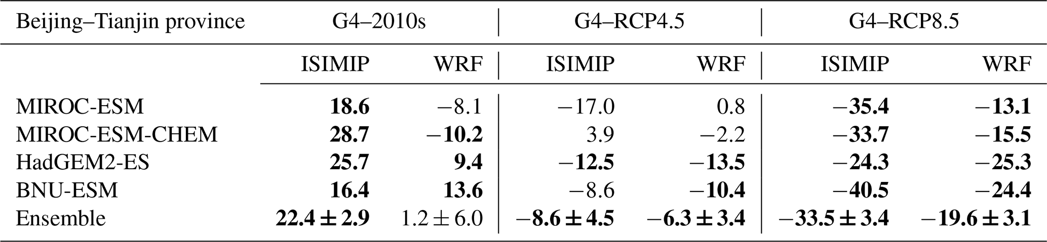
Figure 10 Probability density distributions of daily apparent temperature (AP) in summer (JJA) over Beijing–Tianjin urban areas for a recent period (2008–2017) and the 2060s under G4, RCP4.5, and RCP8.5 scenarios from ISIMIP and WRF. results. The purple dotted lines represent AP of 32 and 39 ^∘C.

3.3 PM_2.5 in the 2060s

3.3.1 PM_2.5 scenarios in the 2060s

We first project the change in PM_2.5 under G4 and the aerosol mitigation scenario in the 2060s relative to the 2010s (Fig. 11a, e). Both ISIMIP and WRF project PM_2.5 decreases in most areas, especially in Tianjin and Langfang, but PM_2.5 decreases more under ISIMIP than WRF. PM_2.5 concentration decreases by 7.6 µg m⁻³ over the Beijing–Tianjin province in ISIMIP and decreases by 5.4 µg m⁻³ in WRF (Table S3). PM_2.5 concentration is 0.5–8 µg m⁻³ higher in northern Beijing under G4 (mitigation) than during the 2010s in WRF. To show the impact of emission reductions, we compare the PM_2.5 concentration between the aerosol baseline and mitigation scenarios under G4 in the 2060s (Fig. 11b, f) and compare the mitigation PM_2.5 concentration under G4 and the RCP scenarios in the 2060s to clarify the effect of geoengineering compared with climate warming. Compared with the baseline scenario, the PM_2.5 concentration is lower under the mitigation scenario, as expected in both ISIMIP and WRF under G4 (Fig. 11b, f), and has a similar spatial pattern to that in Fig. 11a and e. Compared with RCP4.5 and RCP8.5, PM_2.5 concentrations under G4 are higher over the Beijing–Tianjin province in ISIMIP results (Fig. 11c–d), but with large differences between the four ESMs. G4 PM_2.5 is simulated as greater than in RCP scenarios under HadGEM2-ES and BNU-ESM (Fig. S19k, l, o, p), but there are insignificant differences in most areas under the two MIROC models (Fig. S19c, d, g, h). PM_2.5 concentrations are larger between G4 and RCP8.5. WRF simulations show similar changes in PM_2.5 between G4 and RCPs as ISIMIP over the Beijing–Tianjin province (Fig. 11g–h).

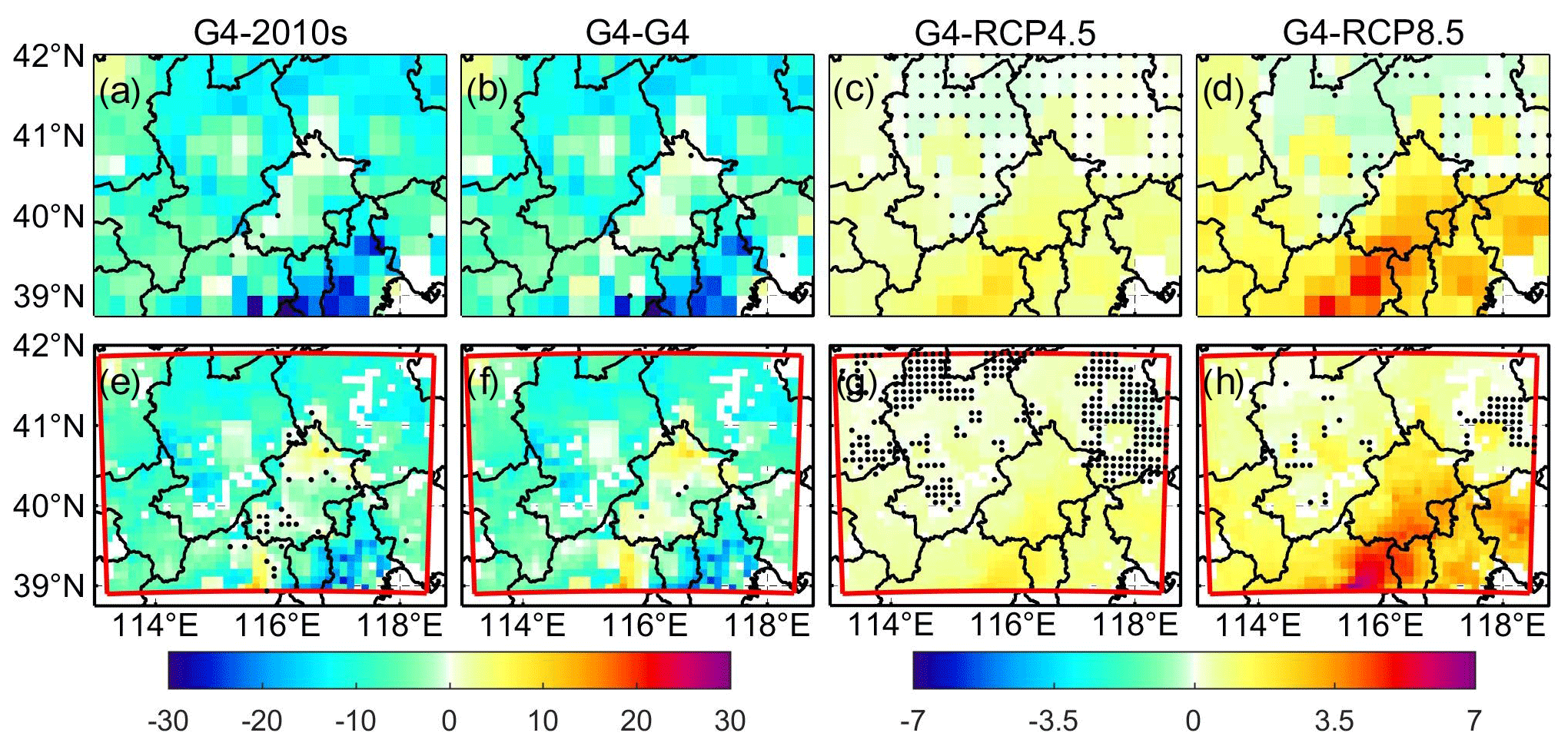
Figure 11 Spatial patterns of ensemble mean PM_2.5 concentration difference (µg m⁻³) between mitigation under G4 in the 2060s and the reference (a, e), between mitigation and baseline under G4 in the 2060s (b, f), between G4 and RCP4.5 under the mitigation scenario in the 2060s (c, g), and between G4 and RCP8.5 under the mitigation scenario in the 2060s (d, h) based on ISIMIP (a–d) and WRF (e–h) results. Excessive collinearity variables have been removed (Fig. S18 shows the results without this procedure). Stippling indicates grid points where differences or changes are not significant at the 5 % significance level according to the Wilcoxon signed rank test.

3.3.2 PM_2.5 meteorological and emission controls in the 2060s

Next, we quantify the contribution of different meteorological factors and PM_2.5 emissions to ΔPM_2.5 for G4 (mitigation) in the 2060s and the 2010s (Fig. 12). Both ISIMIP and WRF results show that the increase in temperature and decrease in PM_2.5 emissions play positive roles in reducing the PM_2.5 concentration. ISIMIP results (Fig. 12a–e) suggest that the projected increase in temperature could explain 0 %–20 % of the decrease in PM_2.5 concentration, and the decrease in PM_2.5 emissions could explain more than 90 % of changes in PM_2.5 concentration differences in most areas. Changes in humidity and westerly winds (positive U wind) do not cause significant changes in ΔPM_2.5, but projected increases in southerly wind (positive V wind) are detrimental to the decrease in PM_2.5 concentration and have a 0 %–10 % negative effect on ΔPM_2.5 in Zhangjiakou. WRF results show a similar spatial pattern for the effect of temperature and emission on ΔPM_2.5 with ISIMIP results. Although temperature is projected to increase over the whole domain (Fig. S22), there are negative contributions to ΔPM_2.5 to the north of Beijing due to an increase in PM_2.5 caused by the negative correlation between PM_2.5 and its emissions (Fig. S26). The ∼1 %–2 % increase in humidity leads to ∼10 % increase in PM_2.5 concentration in the south of Beijing (Fig. 12g), and 0.2–0.3 m s⁻¹ decreases in U wind lead to 0 %–10 % increases in the PM_2.5 concentration in Zhangjiakou (Fig. 12h). The changes in each factor in ISIMIP and WRF results are shown in Figs. S21 and S22, respectively.

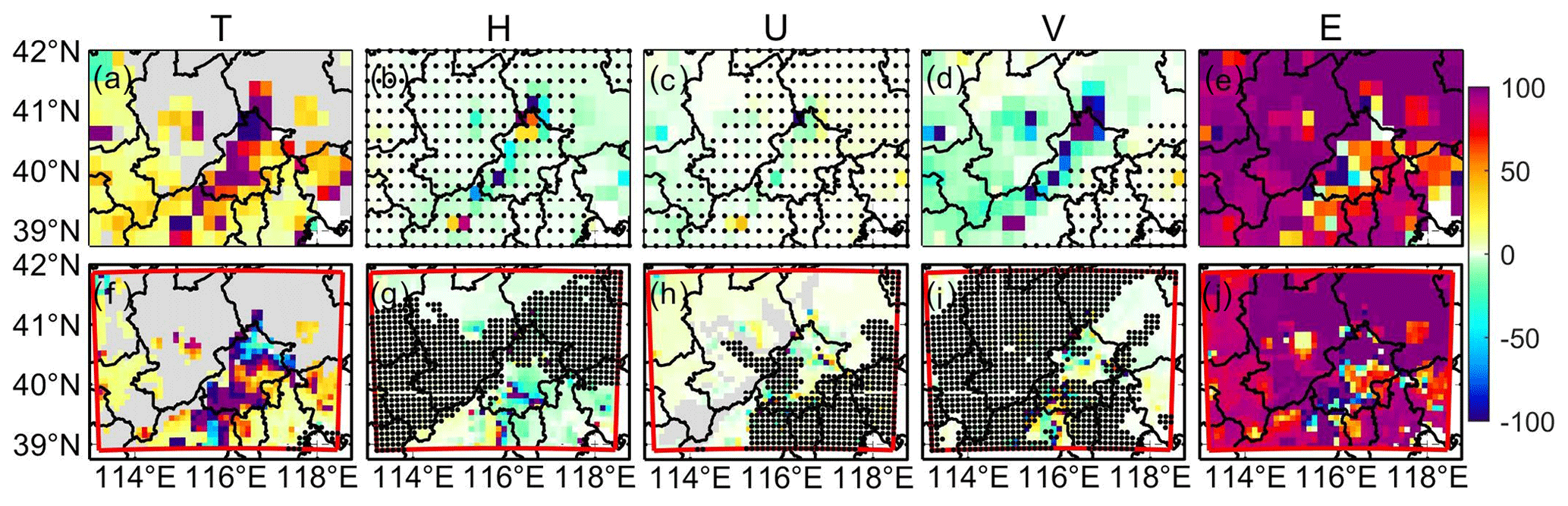
Figure 12 Contribution of climate factors (temperature – T, humidity – H, zonal wind — U, meridional wind – V) and emissions (E) to changes in monthly PM_2.5 concentration (ΔPM_2.5) in the 2060s under G4 (mitigation) relative to the 2010s. Top panels (a–e) are ISIMIP results, and bottom panels (f–j) are WRF results. Stippling indicates that the changes are insignificant at the 5 % significance level in the Wilcoxon test. The grey areas represent the collinearity in the MLR in panels (a), (f), and (h).

Now we explore the contribution of each meteorological factor to ΔPM_2.5 between G4 (mitigation) and RCP4.5 (mitigation) in the 2060s (Fig. 13). The higher PM_2.5 under G4 is mainly caused by the lower temperature. In ISIMIP, lower temperature explains more than 90 % (100 % in some places) of the elevated PM_2.5 relative to RCP4.5, although the increase in humidity is also helpful in lowering PM_2.5 in the western domain (Fig. 13a–b). Humidity can increase suspended particle mass and coagulation, promoting deposition (Li et al., 2015). The contribution of differences in U wind and V wind to ΔPM_2.5 is insignificant (Fig. 13c–d). In WRF, the projected lower temperatures explain more than 70 % of the higher PM_2.5 under G4 relative to RCP4.5 (Fig. 13e). Although the increase in southerly (V) wind contributes 10 %–20 % to the higher PM_2.5 in the northern domain under HadGEM2-ES and BNU-ESM (Fig. S24), it is insignificant in the ensemble (Fig. 13h). Decreased westerlies (U wind) explain between +100 % and −100 % of PM_2.5 differences (Fig. 13g), since U-wind impacts vary spatially (Fig. S26).

3.3.3 PM_2.5 impact on health risks now and in the 2060s

Changes in RR of PM_2.5 for the five diseases under the geoengineering and global warming climate scenarios and different emission scenarios during the 2060s relative to the 2010s for the Beijing–Tianjin province are shown in Fig. 14. Present-day PM_2.5-related RRs are 1.32 (1.30), 1.37 (1.35), 1.46 (1.43), 1.83 (1.80), and 2.03 (1.99) for chronic obstructive pulmonary disease (COPD), ischemic heart disease (IHD), lung cancer (LC), lung respiratory infection (LRI), and stroke according to the ISIMIP (WRF) simulations (Fig. 14a). RR of LRI is the highest and COPD is the lowest for the five diseases, and WRF estimates of RR are 0.02–0.03 lower than those of ISIMIP. In both the baseline and mitigation emission scenarios, RRs will be lower under G4, RCP4.5, and RCP8.5 compared with the 2010s. Smaller RR reductions occur under G4 than under RCP4.5 and RCP8.5, and ISIMIP simulates larger reductions than WRF. This is because the PM_2.5 concentrations from ISIMIP are reduced more than with WRF (Table S3). Under the baseline emission scenario (Fig. 14b–d), the biggest reduction of RR for LRI is 0.047 under RCP8.5 in ISIMIP, and RRs for other diseases are projected to be reduced by no more than 0.02. Under the mitigation emission scenario (Fig. 14e–g), reductions in RRs are 3–6 times greater.

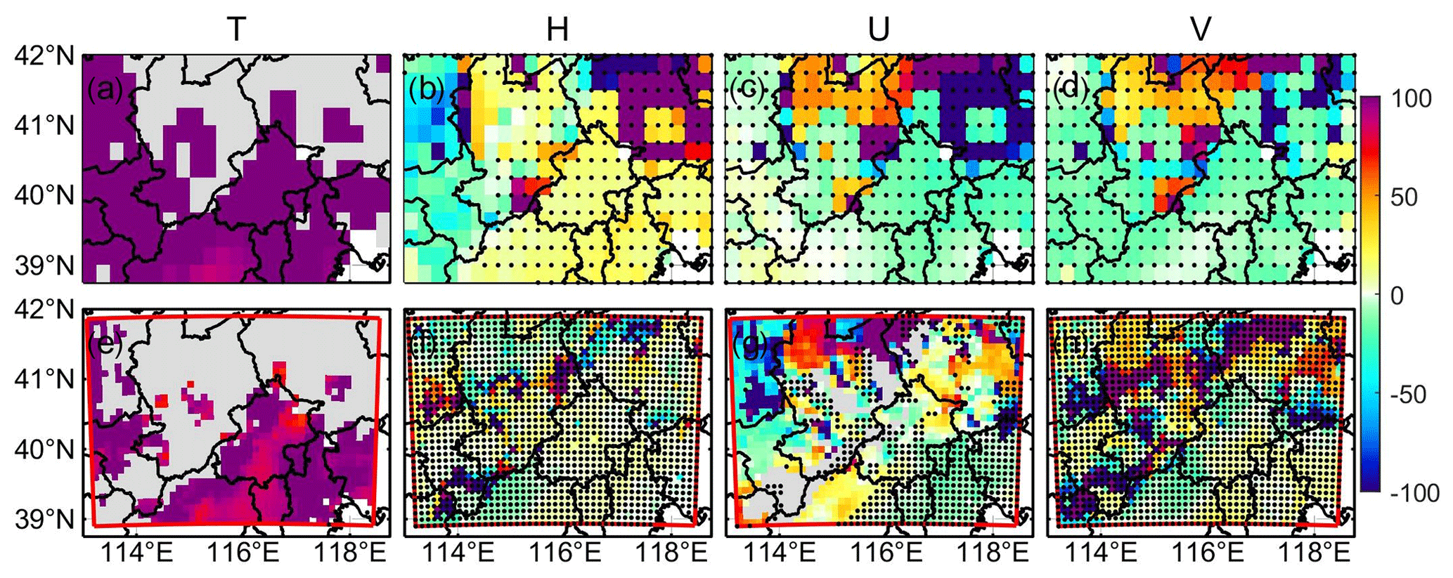
Figure 13 Contribution of climate factors (as in Fig. 12) to changes in monthly PM_2.5 concentration in the 2060s under G4 with aerosol mitigation relative to the 2060s under RCP4.5 with aerosol mitigation. Top panels (a–e) are ISIMIP results, and bottom panels (f–j) are WRF results. Stippling indicates that the changes are insignificant at the 5 % significance level in the Wilcoxon test. The grey areas represent the collinearity in the MLR in panels (a), (f), and (h).

4 Discussion

4.1 Apparent temperature

Both ISIMIP and WRF can reproduce the observed (CN05.1) spatial patterns and seasonal variabilities of apparent temperature in the region around Beijing. WRF shows warm biases in AP during all months relative to CN05.1 due to warmer temperatures in urban areas, with the exception of BNU-ESM and HadGEM2-ES-driven summers (Fig. S13). Both ISIMIP and WRF tend to overestimate population-weighted NdAP_32 by 370 % and 590 %, respectively. These large discrepancies are due to relatively small overestimates of the likelihood of the tails of the probability distributions, which leads to a dramatic increase in the frequency of extreme climate events (Dimri et al., 2018; Huang et al., 2021). AP is about 1.5 ^∘C warmer than 2 m temperature over the Beijing and Tianjin urban areas in summer due to higher vapor pressures amplifying warmer urban temperatures, and this is despite humidity being lower over the cities. Under high-humidity conditions, a slight increase in temperature will cause a large increase in heat stress (Li et al., 2018; Luo and Lau, 2019). AP is nearly 4 ^∘C colder than 2 m temperature in winter due to wind speed (Fig. 2d). Differences between AP and 2 m temperature (AP–T) during summer are greater in urban areas than neighboring rural areas.

The apparent temperatures in Beijing–Tianjin urban areas under G4 in the 2060s are simulated to be 1 and 2.5 ^∘C lower than RCP4.5 and RCP8.5, although AP would be higher than in the recent past. The cooling effect of G4 relative to RCP4.5 and RCP8.5 is the greatest under HadGEM2-ES (Figs. S14, S15) due to the ESM having the largest temperature differences between scenarios (Wang et al., 2022). WRF downscaling produces reduced seasonality in AP compared with ISIMIP, and WRF produces relatively cooler summers and warmer winters than ISIMIP, so there are fewer differences in apparent temperature ranges (Fig. 15). Differences in AP between G4 and the RCP scenarios are mainly driven by temperature. In all scenarios and downscalings AP rises faster than the temperature due to decreased wind speeds in the future (Li et al., 2018; Zhu et al., 2021) but mainly because of rises in vapor pressure driven by rising temperatures. This effect occurs despite the general drying expected under solar geoengineering (Bala et al., 2008; Yu et al., 2015).

The NdAP_32 under G4 is projected to decrease by 8.6 d yr⁻¹ by ISIMIP and 6.3 d yr⁻¹ by WRF relative to RCP4.5 for the Beijing–Tianjin province. Much larger reductions in NdAP_32 of 33.5 d yr⁻¹ (ISIMIP) and 19.6 d yr⁻¹ (WRF) are projected relative to RCP8.5. Differences between scenarios in the frequency of dangerously hot days are far larger using ISIMIP statistical downscaling than using WRF. This is another impact of the reduced seasonality of WRF compared with ISIMIP (Fig. 15).

The higher-resolution WRF simulation produces a much larger range of apparent temperatures across the domain than CN05.1 and ISIMIP downscaling. This increased variability makes reaching a statistical significance threshold more challenging for WRF than ISIMIP results. Despite this, the ESM-driven differences in WRF output are fewer than from ISIMIP, reflecting the physically based processes in the dynamic WRF simulation. This reduces the impact of differences in ESM forcing at the domain boundaries with WRF compared with the statistical bias-correction and downscaling methods. Although there are some uncertainties between models and downscaling methods, G4 SAI can not only reduce the mean apparent temperature but also decrease the probability of PDF tails (extreme events) in summer.

4.2 PM_2.5

We established a set of spatially gridded MLR models based on the four ESMs' downscaled variables under ISIMIP and WRF. The meteorological factors impact PM_2.5 in complex ways, but the simple spatially gridded MLR models display enough skill to make some illustrative projections of future PM_2.5, explaining about 70 % of the variance during the historical period. PM_2.5 concentration is correlated with emissions and anticorrelated with temperature in most parts of the domain (Figs. S25–S26). Increased turbulence increases diffusion of PM_2.5 (Yang et al., 2016), and higher temperatures increase evaporation losses (Liu et al., 2015) of ammonium nitrate (Chuang et al., 2017) and other components (Wang et al., 2006). Humidity may have both positive and negative effects on PM_2.5 (Chen et al., 2020). It causes more water vapor to adhere to the surface of PM_2.5, thereby increasing its mass concentration and facilitating aerosol growth (Cheng et al., 2017; Liao et al., 2017). However, when the humidity exceeds a certain threshold, coagulation and particle mass increase rapidly, promoting deposition (Li et al., 2015). So, the slope coefficients between PM_2.5 and humidity are positive in low-humidity areas, including the southern plain and the Beijing–Tianjin province, but negative in some northern mountain areas (Figs. S25, S26).

There are large spatial differences in wind speed and direction impacts on PM_2.5. Yang et al. (2016) found that weaker northerly and westerly winds tend to increase the PM_2.5 concentration in northern and eastern China, respectively. The effects of wind direction depend on the distribution of emitted PM_2.5 and the condition of the underlying surface (Chen et al., 2020). Most sources of PM_2.5 lie to the south of our domain, and relatively clean conditions prevail to the north, so northerly winds tend to advect clean air, while southerlies bring high concentrations of aerosols. Weak winds tend to increase PM_2.5 and smog formation due to sinking air and weak diffusion (Ren et al., 2016; Yang et al., 2018).

Xu et al. (2021) projected that 2030 PM_2.5 concentrations will decrease by 8.8 % and 5.5 % under RCP4.5 and RCP8.5, respectively, relative to 2015. Y. Wang et al. (2021) also projected decreasing trends in China under RCP4.5 and RCP8.5 during 2030–2050. There were seasonal changes in PM_2.5 concentration differences between two RCPs (RCP4.5 and 8.5) and the historical scenario near the Bohai Sea (Dou et al., 2021). However, there are also some simulations wherein PM_2.5 concentrations increase in warmer climates. Hong et al. (2019) suggest that annual mean PM_2.5 concentrations will increase by 1–8 µg m⁻³ in an area including Beijing and Tianjin under RCP4.5 during 2046–2050 compared with 2006–2010. These inconsistent responses are mainly caused by the differences in the selection of ESMs, chemical transport models, and climate–emission scenarios. Different RCP scenarios not only correspond to different future climate states, but also have different anthropogenic emissions of air pollutants. In our study, we do not consider the PM_2.5 emission differences between RCP4.5 and RCP8.5, and we instead applied the ECLIPSE PM_2.5 emission scenarios in our MLR projection.

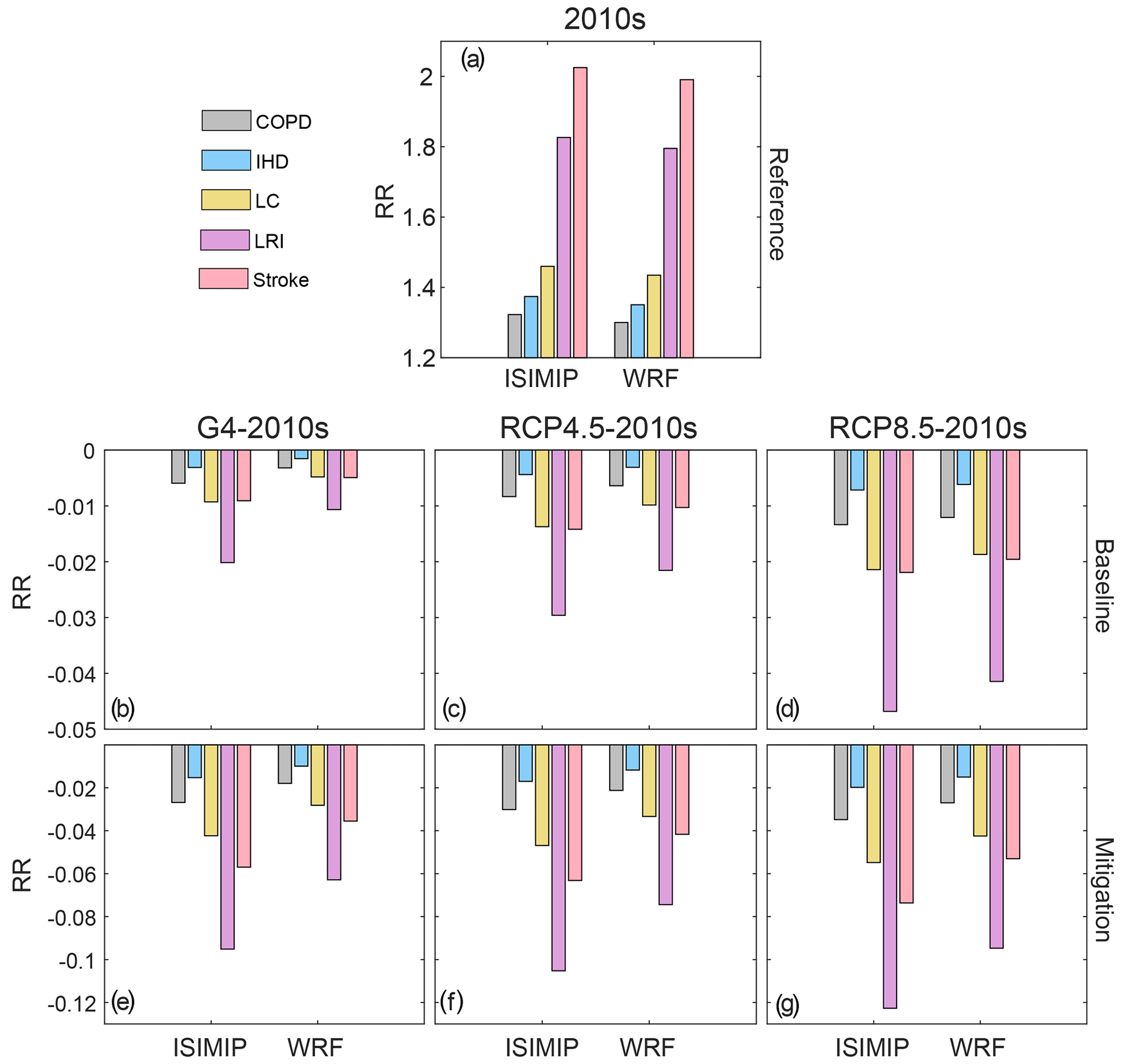
Figure 14 Average population-weighted relative risks of five PM_2.5-related diseases in the 2010s (a) and changes between G4 and the 2010s (b, e), between RCP4.5 and the 2010s (c, f), and between RCP8.5 and the 2010s (d, g) in the Beijing–Tianjin province based on the ISIMIP and WRF results, respectively. PM_2.5 concentration is based on the baseline emissions under G4, RCP4.5, and RCP8.5 in the middle three panels (b–d), and it is based on the mitigation emissions under G4, RCP4.5, and RCP8.5 in the bottom three panels (e–g).

Emissions reductions are expected to play the dominant role in the decrease in PM_2.5 concentrations under G4 aerosol mitigation in the 2060s (Fig. 12). Meteorological changes under the different future scenarios make much smaller changes as evidenced by the scenarios using the baseline – that is, present-day PM_2.5 emissions, with decreases in mean annual concentrations of 1.0 (1.3), 1.8 (2.0), and 3.3 (3.2) µg m⁻³ over the Beijing–Tianjin province under G4, RCP4.5, and RCP8.5 with WRF (ISIMIP) (Table S3), which are mainly caused by the temperature increases (Fig. 13). The negative relationships between emissions and the PM_2.5 concentration result in the increase in PM_2.5 under G4 (mitigation) relative to the 2010s in the north of Beijing with WRF. This may be due to changes in PM_2.5 out of the domain being opposite to those in the domain during the MLR fitting period, since relocation of polluting sources from the urban areas mainly to the west occurred over the calibration period. The accuracy of PM_2.5 emission data is also crucial for training MLR models, and PM_2.5 data were sparse before 2013, relying on reconstructions based on satellite optical depth estimates. Although both increases in temperature and decreases in emissions explain more than 90 % of the decrease in PM_2.5 in most areas, there are large spatial differences due to wind and humidity. On the one hand, there is uncertainty in the differences in changes in wind speed and humidity between different ESMs and downscaling methods; on the other hand, the complex physical relationship between them and PM_2.5 also increases uncertainties. Reductions in PM_2.5 in the future are projected to decrease PM_2.5-related health issues, although the effects on various diseases are different. Changes in PM_2.5-related risk between G4 and RCPs are from 1 %–3 %, with PM_2.5 emissions policy dominating differences over the climate scenario.

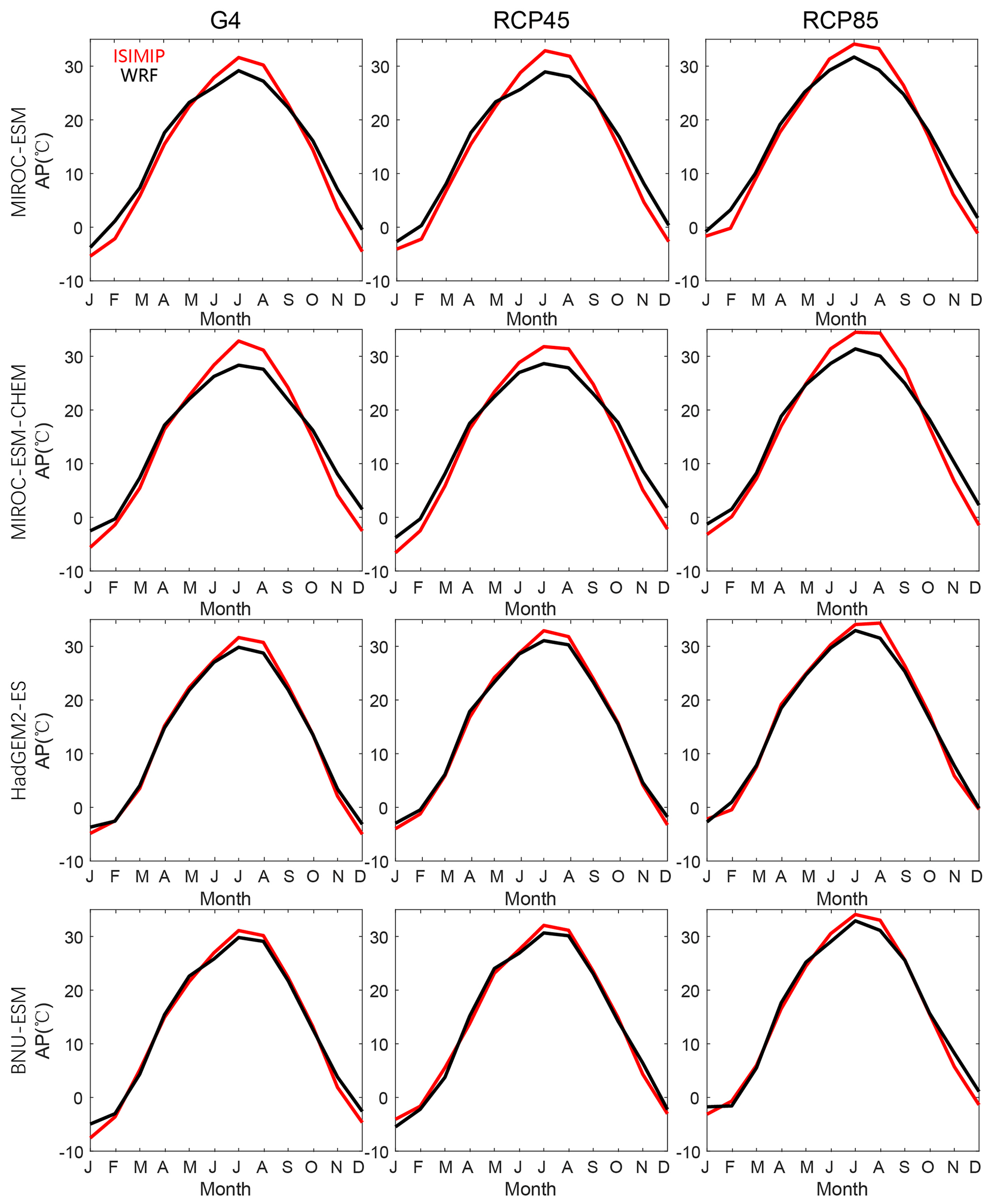
Figure 15 Seasonal cycles of apparent temperature from MIROC-ESM, MIROC-ESM-CHEM, HadGEM2-ES, and BNU-ESM under G4, RCP4.5, and RCP8.5 in Beijing–Tianjin urban areas during the 2060s based on ISIMIP (red) and WRF (black) methods.

There are some differences in projecting PM_2.5 concentrations between WRF and ISIMIP methods. Compared to the 2010s reference, PM_2.5 concentrations in ISIMIP are projected to decrease more than using WRF in G4 under the mitigation scenario during the 2060s over the Tianjin province (Fig. 11a, e). However, the spatial patterns of changes in PM_2.5 concentration between G4 and two RCPs (RCP4.5 and 8.5) under the mitigation scenario during the 2060s are similar (Fig. 11c–d, g–h). This means that the effects of different downscaled methods on projecting PM_2.5 are small if we only consider climate change alone without considering emissions changes. Due to the larger regression coefficient of emissions in the MLR under the ISIMIP method (Figs. S25, S26), the negative changes in PM_2.5 concentration are larger between mitigation and baseline under G4 during the 2060s than that under the WRF method. Correspondingly, the ISIMIP method has a greater reduction in PM_2.5-related RR than WRF under three future climate scenarios during the 2060s.

Eastham et al. (2018) deduced from experiments using 1 Tg yr⁻¹ SAI in a coupled chemistry–transport model directly simulating atmospheric chemistry, transport, radiative transfer of UV, emissions, and loss processes that per unit of mass emitted, surface-level emissions of sulfate result in 25 times greater population exposure to PM_2.5 than emitting the same aerosol into the stratosphere. The G4 experiment specifies a 5 Tg yr⁻¹ injection rate, which over our domain would equate to 1450 t yr⁻¹ if it was deposited uniformly globally (which it certainly would not be). Reducing this by a factor of $\mathrm{1}/\mathrm{25}$ amounts to 58 t yr⁻¹, which can be compared with present PM_2.5 emissions of around 3.3×10⁵ t yr⁻¹ in our domain. If we consider the aerosol deposition under G4 scenarios, the PM_2.5 concentration will be 0–1 µg m⁻³ higher than that without due to deposition of the SAI aerosols (Fig. S27), and RR is projected to increase by 0.01 % for the Beijing–Tianjin province (Table S4). This comparison suggests that tropospheric emissions will be much more important for human health in our domain than from the SAI specified by G4.

The most important change in PM_2.5 will come from emissions reductions, with the different weather conditions under both G4 and RCP scenarios making relatively little practical difference in concentrations. PM_2.5 concentration is expected to decrease significantly (ISIMIP: −7.6 µg m⁻³, WRF: −5.4 µg m⁻³) in the Beijing–Tianjin province, but they will still not meet Chinese or international standards. The temperature under G4 is lower than that under RCP4.5 and RCP8.5 scenarios, which makes the PM_2.5 concentration under G4 higher. But the difference in PM_2.5 between the two is small and even within uncertainty due to projected differences in humidity and wind. Potentially improved estimates from more complex models such as WRF-Chem, CMAQ, and GEOS-Chem over the simple MLR methods used here will be of limited value unless the differences between the ESMs driving these models are reduced. It can be confirmed that emission policies based on the 13th Five-Year Plan are not enough, and higher emission standards need to be developed for a healthy living environment.

Our study did not consider the impacts of socioeconomic pathways on PM_2.5 future emissions; instead, we explore the meteorological differences between the SAI G4 scenario and the greenhouse gas scenarios (RCP4.5 and RCP8.5) in terms of the impact on PM_2.5 concentrations. PM_2.5 emissions were defined by the uncontrolled scenario (baseline) and a scenario in which technological intervention (mitigation) reduces emissions. There are some limitations in our study. Firstly, the HTAP_V3 dataset only includes anthropogenic PM_2.5 emissions, not natural PM_2.5 emissions. Natural PM_2.5 will also change in the future under changing climate. The sources of natural PM_2.5 include the sandstorms that sometimes occur in spring as extreme winds mobilize dry unvegetated soils. These relatively extreme conditions are difficult to simulate in ESMs and subject to land use policy – e.g., the numerous ecosystem service measures undertaken by China over the last 5 decades (Miao et al., 2015). Secondly, although PM_2.5 concentration includes both primary and secondary PM_2.5 during model training, we do not consider the precursor gases for secondary PM_2.5 directly. The sensitivity of MLR may be diminished at high PM_2.5 values when secondary PM_2.5 dominates the variability of total PM_2.5 (Upadhyay et al., 2018). Thirdly, we only consider the effect of dominant near-surface meteorological variables on PM_2.5. However, the vertical transport of pollutants related to vertical atmospheric stability should not be ignored (Lo et al., 2006; Wu et al., 2005), and this may contribute to the differences in the RCP4.5 scenario from our MLR model and more sophisticated simulations (Fig. S7). Finally, although it is insignificant for the Beijing and Tianjin provinces, the MLR model suffers from collinearity problems in some areas. These factors play smaller roles as we are mainly considering changes in PM_2.5 concentrations between different climate scenarios. Nevertheless, projection for changes in PM_2.5 between SAI scenarios and per greenhouse gas scenario would be valuable for global air quality impacts from geoengineering.

5 Conclusions

Our study on thermal comfort and aerosol pollution under geoengineering scenarios for the Beijing megalopolis may be useful across the developing world, which is expected to suffer from disproportionate climate impact damage relative to the global mean, while also undergoing rapid urbanization. Assessing health impacts and mortality due to heat stress and PM_2.5 under greenhouse gas scenarios should consider urbanization and the change to concrete surfaces from vegetation that leads to differences in heat capacities, rates of evapotranspiration, and hence humidity and apparent temperature. These require downscaled analyses, accurate meteorological and high-resolution land surface datasets, and industrial development scenarios.

In our analysis we assumed the urban area did not change over time and also that the population remains distributed as in the recent past. This may be reasonable in the highly developed and relatively mature greater Beijing–Tianjin region but should be considered in rapidly urbanizing regions elsewhere. There certainly will be changes over time in the radiative cooling from surface pollution sources. PM_2.5 is a health issue in many developing regions (Ran et al., 2023), but as wealth increases efforts to curb air pollution generally clean the air. This has clear health benefits but also removes aerosols from the troposphere that cool the surface. The urban areas that have higher apparent temperatures at present are also the areas with the greatest aerosol load and hence the greatest cooling. Once direct radiation is removed, air temperatures and apparent temperatures will all rise by several degrees (Wang et al., 2016). So, a future more comprehensive health impact study would include both the negative health impacts of aerosol pollution and the potential cooling effects those aerosols produce. Additionally, the formulation of apparent temperature used does not consider the effect of radiation on human comfort (Kong and Huber, 2022). When PM_2.5 levels are high there is no shade because the sky is milky white; similarly, SAI will brighten the sky (Kravitz et al., 2012). Comfort is increased in clear-sky conditions when shade is readily found.

The changes simulated to relative risk from increased PM_2.5 under the G4 SAI scenario are about 1 %–3 % worse than under RCP4.5, mainly because of lower temperatures under G4. The difference this would make to the overall health burden under SAI depends on the range of other impacts that include changes in apparent temperature we discuss. G4 reduces the number of days with AP > 32 (when extreme caution is advised) by 6–8 per year relative to RCP4.5 and by 20–34 relative to RCP8.5. But G4 itself will still increase these extreme caution days by 1–20 relative to conditions in the 2010s. Lowering PM_2.5 emissions will increase ground temperatures, and the associated risk of dangerous apparent temperatures will also increase rapidly as the distribution of temperatures is shifted, making presently rare hot events into much more frequent heat waves.