Combining local model calibration with the emergent constraint approach to reduce uncertainty in the tropical land carbon cycle feedback

The role of the land carbon cycle in climate change remains highly uncertain. A key source of the projection spread is related to the assumed response of photosynthesis to warming, especially in the tropics. The optimum temperature for photosynthesis determines whether warming positively or negatively impacts photosynthesis, thereby amplifying or suppressing CO₂ fertilisation of photosynthesis under CO₂-induced global warming. Land carbon cycle models have been extensively calibrated against local eddy flux measurements, but this has not previously been clearly translated into a reduced uncertainty in terms of how the tropical land carbon sink will respond to warming. Using a previous parameter perturbation ensemble carried out with version 3 of the Hadley Centre coupled climate–carbon cycle model (HadCM3C), we identify an emergent relationship between the optimal temperature for photosynthesis, which is especially relevant in tropical forests, and the projected amount of atmospheric CO₂ at the end of the century. We combine this with a constraint on the optimum temperature for photosynthesis, derived from eddy covariance measurements using the adjoint of the Joint UK Land Environment Simulator (JULES) land surface model. Taken together, the emergent relationship from the coupled model and the constraint on the optimum temperature for photosynthesis define an emergent constraint on future atmospheric CO₂ in the HadCM3C coupled climate–carbon cycle under a common emissions scenario (A1B). The emergent constraint sharpens the probability density of simulated CO₂ change (2100–1900) and moves its peak to a lower value of 497 ± 91 compared to 607 ± 128 ppmv (parts per million by volume) when using the equal-weight prior. Although this result is likely to be model and scenario dependent, it demonstrates the potential of combining the large-scale emergent constraint approach with a parameter estimation using detailed local measurements.

1 Introduction

One of the key sources of uncertainty in future climate projections is the evolution of the land carbon sink (Friedlingstein et al., 2006; Cox et al., 2000; Arora et al., 2020; Canadell et al., 2021). As climate change elevates global temperatures and CO₂ conditions, the rate and efficiency of vegetation photosynthesis and respiration changes, influencing the capacity of the land to act as a repository for anthropogenic CO₂ (Medlyn et al., 1999; Cox et al., 2000; Friedlingstein et al., 2006). The structure and distribution of vegetation may also change in response to the associated climate change, such as changes in precipitation patterns (Trenberth, 2011). These responses provide feedback on the initial climate change signal, potentially leading to key transitions and tipping points in the land biosphere. Notable examples include a global carbon sink-to-source transition, Amazon rainforest dieback (Cox et al., 2004), shifting of the boreal forests (Chapin et al., 2004), and greening of the Sahel (Claussen et al., 2002).

Despite the increasing complexity of the climate–carbon cycle models developed for the latest IPCC (International Panel on Climate Change) Assessment Report (AR6), there is still a significant spread in the projections of vegetation and soil carbon under common trajectories of atmospheric greenhouse gases and aerosols (Canadell et al., 2021). This spread arises partly from different climate projections within the host climate model and partly from uncertainties in the land surface models themselves. Indeed, for the Joint UK Land Environment Simulator (JULES) land surface model (Clark et al., 2011; Best et al., 2011) under one of the IPCC Special Report on Emissions Scenarios (SRES – A1B; Nakicenovic et al., 2000), the atmospheric CO₂ change by the end of the century (ΔCO₂) was found to range from 373.8 to 845.7 ppmv (parts per million by volume; Booth et al., 2012). This range was achieved simply by perturbing some of the model parameters related to the sensitivities of plant photosynthesis and soil respiration to temperature, stomatal conduction, soil water availability and surface evaporation, and plant competition. The key source of projection spread was found to be related to the assumed response of photosynthesis to warming, especially in the tropics (Kattge and Knorr, 2007; Booth et al., 2012; Cox et al., 2013; Mercado et al., 2018). Indeed, the optimum temperature for photosynthesis (T_opt) is a common parameter in land surface models that determines whether warming has a positive or negative impact on photosynthesis, thereby either amplifying or suppressing the CO₂ fertilisation of photosynthesis under CO₂-induced global warming (Friedlingstein et al., 2006; Arora et al., 2020).

There is an urgent need to reduce such parametric uncertainties to make reliable and believable climate projections. Usually, to reduce uncertainty in model simulations, models are confronted with observations. However, although there is now an unprecedented volume of in situ and Earth observation (EO) data with which to confront the models, the relatively shorter timescales mean that these cannot be directly used to create constraints on changes in the Earth system over the next century. Furthermore, it is extremely computationally expensive to run complex land carbon cycle models (also known as land surface models or LSMs), within Earth system models (ESMs) to produce multiple climate–carbon cycle projections. Instead, computationally efficient ways to translate short-term constraints into reductions in the long-term projection uncertainty need to be developed.

Emergent constraints are used to bridge the gap between short-term contemporary observations and long-term future predictions (Cox et al., 2013; Wenzel et al., 2014, 2016; Hall et al., 2019; Williamson et al., 2021). Using the constraints provided by the observations and physical understanding available today, emergent constraints can be used to assess the relative likelihood of different long-term trends (Allen and Ingram, 2002). Emergent constraints identified in the carbon cycle include the sensitivity of the annual growth rate of atmospheric CO₂ to tropical temperature anomalies (Cox et al., 2013) and the changing amplitude of the CO₂ seasonal cycle to the projected land photosynthesis (Wenzel et al., 2016; Hall et al., 2019; Williamson et al., 2021).

Data assimilation (DA) has been shown to be a useful and versatile tool to constrain the response of the carbon cycle in LSMs in the short term. DA techniques use contemporary observations to improve the performance of a model by optimising two different components, which are either the values of unknown parameters (parameter estimation) or the predictions of the model according to a given dataset (state estimation). In both cases, this is achieved by trying to find an optimal match between the model and the observations by varying the properties of the model. In numerical weather prediction, DA has predominantly been used to optimise the state whilst keeping the parameters fixed. This is because the physics are mostly known and well-understood. However, in terrestrial carbon cycle models, where most of the equations are unknown, finding the correct set of parameters is more pertinent. These models can have over a hundred internal parameters representing the environmental sensitivities of the various land surface and plant functional types. These parameters are generally chosen to represent measurable real-world quantities (e.g. surface albedo and plant root depth). This allows observationally based estimates of these parameters to be made in the early stages of the model development process. However, the detailed performance of an LSM can be very sensitive to such internal parameters, and so it is common for land surface modellers to calibrate their models against available observations. Since optimisations give the best possible values of the parameters, given the model parameterisation and structural errors, the results are more reliable than field measurements of the same parameters, which are often taken at different spatial scales than the model resolution.

In this study, we show how we can combine parameter optimisation with emergent constraint techniques to reduce uncertainty in future projections. Specifically, we derive an emergent constraint between a linear regression across the possible JULES T_opt values between the change in CO₂ by the end of the century (ΔCO₂), and the posterior distribution of parameter T_opt optimised against gross primary productivity (GPP) and latent heat (LE) in situ measurements.

2 Methods

2.1 A relationship between T_opt and ΔCO₂

In Booth et al. (2012)'s study, a large range of climate–carbon cycle feedbacks was found by perturbing the model parameters in the land surface component of the Hadley Centre coupled climate model (version 3; HadCM3C). This experiment was conducted under the common climate scenario, A1B, which describes a future world of very rapid economic growth, a global population that peaks in the mid-century and declines after that, and the rapid introduction of new and more efficient technologies, with a balance of fossil-intensive and non-fossil energy sources (Nakicenovic et al., 2000). One of the parameters perturbed in Booth et al. (2012) was T_opt, which corresponds to the optimal temperature for non-light-limited photosynthesis for broadleaf forests. In JULES, non-light-limited leaf-level photosynthesis is controlled by the carboxylation rate, following the models of Collatz et al. (1991, 1992), with T_opt representing the temperature at which the carboxylation rate reaches a maximum. This parameter was identified as being the most important in controlling the carbon response of the model. Indeed, a statistically highly significant (p=0.000153) relationship between T_opt and net CO₂ change by 2100 (ΔCO₂) was found, whereas the rest of the parameters perturbed in the experiment showed little to no correlation with this change (Booth et al., 2012). T_opt and ΔCO₂ were shown to be anti-correlated, with higher values of T_opt resulting in lower values of ΔCO₂. This implies that when the optimal temperature for photosynthesis for broadleaf trees is high, more CO₂ is predicted to be removed from the atmosphere through increased CO₂ fertilisation. This is particularly relevant in the tropics, where in a warming world, ambient temperatures have the potential to exceed the optimal photosynthetic temperature persistently and where broadleaf trees represent large carbon stocks (Booth et al., 2012).

Using linear regression, we can exploit this relationship to calculate a probability distribution function (PDF) for the distribution of ΔCO₂ given T_opt; i.e. P{ΔCO₂|T_opt}. The contours of equal probability density around the best-fit linear regression follow a Gaussian probability density.

$$\begin{array}{}\text{(1)}& P\mathit{\left\{}\mathrm{\Delta }{\mathrm{CO}}_{\mathrm{2}}\right|T_{\mathrm{opt}}\mathit{\}}={\displaystyle \frac{\mathrm{1}}{\sqrt{\mathrm{2}\mathit{\pi }{\mathit{\sigma }}_f^{\mathrm{2}}}}}\exp \left\{-{\displaystyle \frac{{\left(\mathrm{\Delta }{\mathrm{CO}}_{\mathrm{2}}-f\left(T_{\mathrm{opt}}\right)\right)}^{\mathrm{2}}}{\mathrm{2}{\mathit{\sigma }}_f^{\mathrm{2}}}}\right\},\end{array}$$

where f is the function describing the linear regression between ΔCO₂ and T_opt, and σ_f is the prediction error in the regression.

2.2 A constraint on T_opt using local eddy flux measurements

The land surface component of HadCM3C was the Met Office Surface Exchange Scheme (MOSES; Cox et al., 1999), which became the Joint UK Land Environment Simulator (JULES). The adJULES system (Raoult et al., 2016) was developed specifically to optimise the internal parameter of the JULES land surface model using data assimilation. Data assimilation allows the integration of multiple types of data (y) in order to optimise the model parameters (x), while making allowance for associated uncertainties. It is a powerful tool which allows for objective and repeatable calibrations. A Bayesian framework is used to include prior knowledge about the parameters (x_b). All errors are assumed to be Gaussian distributed (with R and B as the prior error covariance matrices for the observations and parameters, respectively). The optimisation corresponds to minimising the mismatch (J) between the model outputs and the observed data with respect to x as follows:

$$\begin{array}{}\text{(2)}& \begin{array}{rl}J\left(\mathit{x}\right)& ={\displaystyle \frac{\mathrm{1}}{\mathrm{2}}}[{\left(\mathit{y}-M\left(\mathit{x}\right)\right)}^T{\mathbf{R}}^{-\mathrm{1}}\left(\mathit{y}-M\left(\mathit{x}\right)\right)\\ & -{\left(\mathit{x}-{\mathit{x}}_{\mathrm{b}}\right)}^T{\mathbf{B}}^{-\mathrm{1}}\left(\mathit{x}-{\mathit{x}}_{\mathrm{b}}\right)],\end{array}\end{array}$$

where M(x) is the model output vector given x. Methods for minimising the cost function range from stochastic random search algorithms to deterministic gradient-based methods.

This second class of methods was integrated into the adJULES system (Raoult et al., 2016). The adJULES system uses the adjoint of the JULES model, a computationally efficient way used to calculate the gradient of Eq. (2). The adjoint allows for efficient and repeatable optimisations utilising the gradient information. The quasi-Newton algorithm L-BFGS-B (limited memory Broyden–Fletcher–Goldfarb–Shanno algorithm with bound constraints; see Byrd et al., 1995) is used to minimise the cost function iteratively. At each iteration of the algorithm, the cost function and its gradient with respect to each parameter are evaluated. The adjoint also allows for the accurate calculation of the Hessian (second derivative of the cost function) at the optimum. The Hessian determines the posterior error covariance matrix, which is used to calculate the posterior uncertainties associated with the best-fit parameters (in the form of PDFs).

Deriving the adjoint of a model as complex as JULES is extremely costly. Fortunately, this has been done for JULES v2.2, which uses the same photosynthesis model as MOSES, allowing us to optimise the same parameters and photosynthesis model as used in HadCM3C and, therefore, in Booth et al. (2012)'s perturbation experiment. In Raoult et al. (2016), adJULES was used to improve the model performance at a wide range of broadleaf sites by optimising the key land surface parameters perturbed in Booth et al. (2012). Each parameter was assigned a wide prior distribution, allowing the parameters to take values from a large range of credible values elicited from expert opinion. The optimisation was performed using monthly in situ GPP and LE data from CO₂ eddy fluxes measured at FluxNet sites (Baldocchi et al., 2001; Pastorello et al., 2020). The FluxNet database contains more than 500 locations worldwide, and all of the data are processed in a harmonised manner, using the standard methodologies including correction, gap-filling, and partitioning (Papale et al., 2006). A large number of broadleaf sites was selected from this database (27 in total; see Raoult et al., 2016, for details). The optimisation was performed in a multi-site configuration, i.e. simultaneously over all selected sites, and over both fluxes to find a single set of best-fit model parameters and their associated uncertainties. The optimisation returned best-fit parameters with posterior distributions much narrower than the prior, thereby reducing the range of viable parameter values. From these posterior distributions, we obtain an observationally constrained PDF for T_opt (i.e. P(T_opt)).

2.3 Calculation of the PDF for ΔCO₂

We follow the method used by Cox et al. (2018) to bring these two elements together and calculate the PDF for ΔCO₂. The PDF for ΔCO₂ is calculated by numerically integrating over the product of two PDFs, namely P{ΔCO₂|T_opt} and P(T_opt).

$$\begin{array}{}\text{(3)}& P\left(\mathrm{\Delta }{\mathrm{CO}}_{\mathrm{2}}\right)=\underset{-\mathrm{\infty }}{\overset{\mathrm{\infty }}{\int }}P\mathit{\left\{}\mathrm{\Delta }{\mathrm{CO}}_{\mathrm{2}}\right|T_{\mathrm{opt}}\mathit{\}}P\left(T_{\mathrm{opt}}\right)\mathrm{d}{T}_{\mathrm{opt}}.\end{array}$$

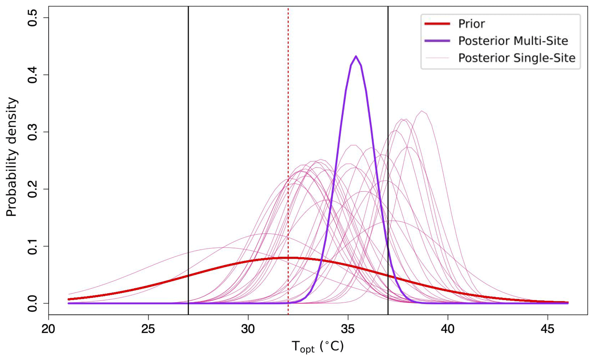
Figure 1 Different PDFs of P(T_opt) found when using the adJULES system to optimise the JULES land surface model against FluxNet data. The prior distribution (red) of the parameter is compared to the posterior distribution (purple) found by simultaneously calibrating over the 27 broadleaf FluxNet sites considered in Raoult et al. (2016, i.e. a multi-site optimisation) and the individual posterior distributions found by calibrating at each site separately (i.e. single-site optimisations). All distributions are modelled by a Gaussian curve. Note that the range used in the optimisation (entire x axis) is greater than the range used in Booth et al. (2012, vertical black lines). The initial value of T_opt in JULES is highlighted by the dashed red line.

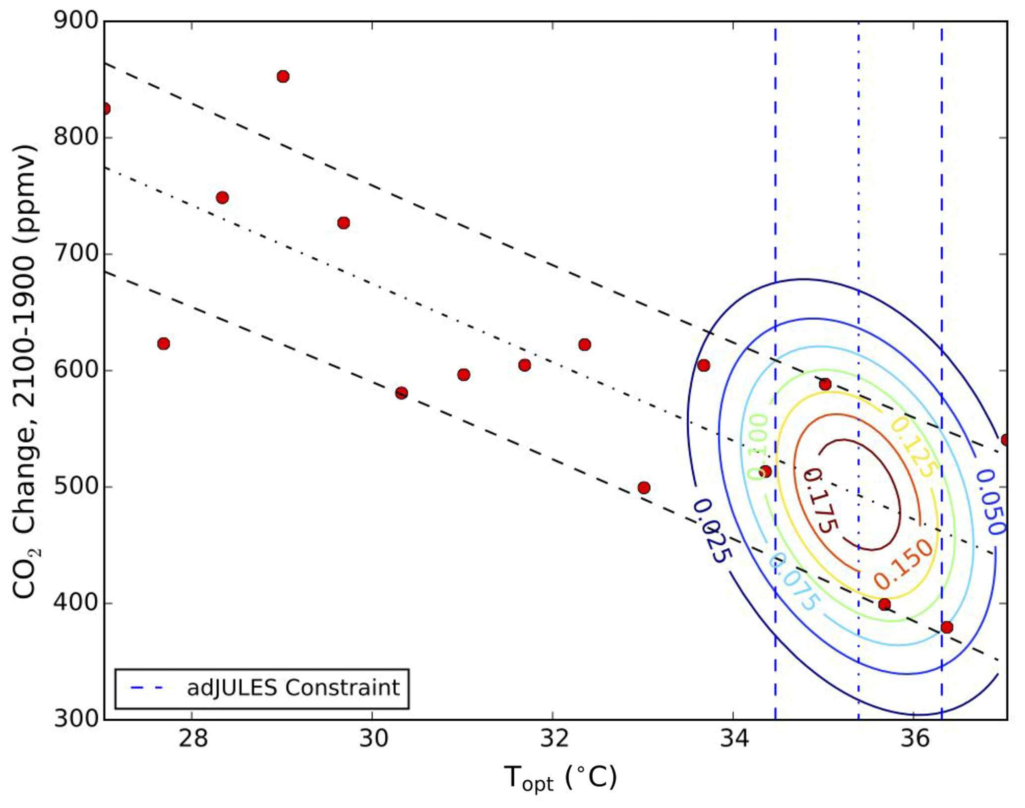
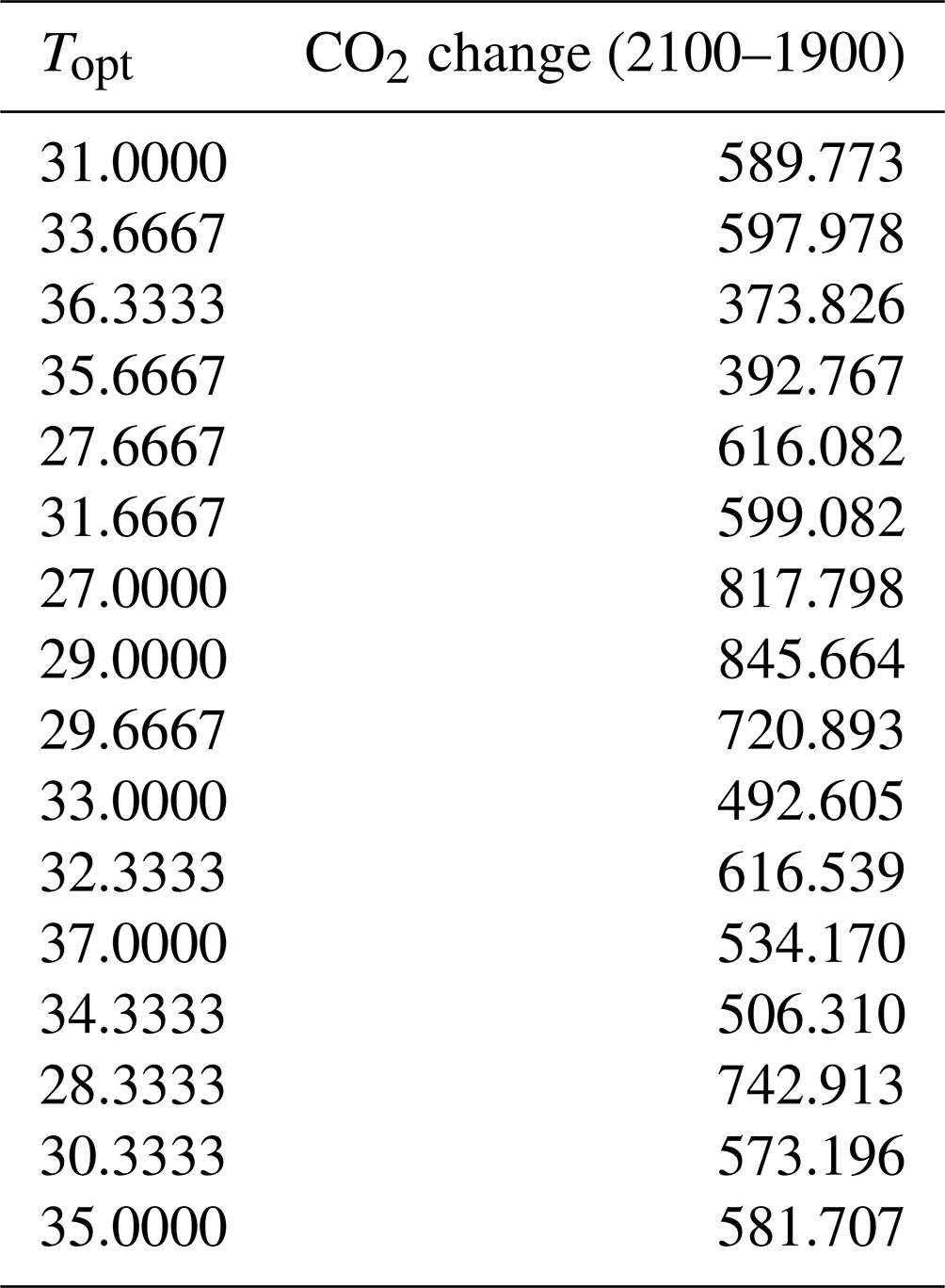
Figure 2 Contours of the probability density for the linear regression adapted from Booth et al. (2012). The red dots show the relationship between different T_opt values and the resulting change in CO₂ by the end of the century from the parameter perturbation experiment of Booth et al. (2012, see Table A1 for these values). The thin dashed black line shows the best-fit linear regression, and the thick dashed black lines on either side show the best-fit linear regression plus and minus the prediction error (see Sect. 2). The vertical blue lines show the observational constraint on the T_opt value, with the best fit shown by the thin dashed blue line, and the thick vertical dashed lines on either side showing plus and minus 1 standard error about this value. The continuous contours are the product of these two underlying PDFs. The integral of these contours across the x-axis variable leads to the T_opt-constrained PDF shown in Fig. 3a.

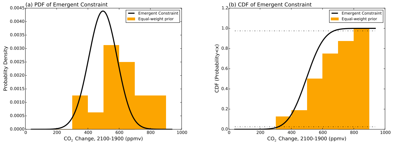
Figure 3 Emergent constraint on the sensitivity of T_opt to the magnitude of the future carbon cycle response. The probability density histogram for the unconstrained T_opt values (orange) and the conditional PDF arising from the emergent constraint (black) are shown in panel (a) and the corresponding cumulative distribution in panel (b). The horizontal dotted–dashed line shows the 95 % confidence limits on the cumulative density function (CDF) plot. The orange histograms (both panels) show the prior distributions that arise from the equal weighting of the parameter perturbation experiment in 500 ppmv bins.

3 Results and discussion

Figure 1 shows how the distribution of likely T_opt values, i.e. P(T_opt), changes when the JULES LSM is optimised against local measurements of photosynthesis (GPP) and latent heat (LE) using the adJULES system (Raoult et al., 2016). We can see that the posterior distribution is much more pronounced than the prior and suggests a higher parameter value than previously used. Values of T_opt taken from this distribution, when used in the JULES model, will result in the best fit of the model to local measurements of photosynthesis (GPP) and latent heat (LE) and therefore improve the model's credibility.

In addition to displaying the results found by optimising simultaneously over all of the broadleaf sites found in Raoult et al. (2016), Fig. 1 also considers distributions of T_opt found when optimising at each individual broadleaf site. Though none of these gives such a narrow distribution, the majority do suggest that the optimal value for the parameter (shown by the peak of the distributions) is higher than previously used in the JULES model. This gives confidence in the posterior distribution found by calibrating over all sites. Furthermore, one of the known limitations of gradient-based methods is their tendency to become stuck in local minima (i.e. not finding the “true” global minimum). Optimisations over multiple sites have been shown to be more robust, with the additional constraints from each site acting to smooth the cost function, thus making local minima less common. As such, multi-site optimisations are more reliable for finding the true best-fit parameters and associated PDFs. For the remainder of this study, we will solely use the posterior distribution found by calibrating over all sites.

Through this multi-site calibration, we find T_opt (i.e. the optimal temperature for non-limited photosynthesis for broadleaf forests) to be around 35 ^∘C, with an uncertainty of approximately ± 0.9 ^∘C. This value falls well within the typical 30–40 ^∘C temperature range observed in most leaf-scale photosynthetic-temperature response curves (Kattge and Knorr, 2007). However, land surface models are not commonly run at the leaf scale – especially not when run within wider Earth system models to predict climate change. Furthermore, T_opt at the leaf scale has been shown to differ from T_opt at ecosystem level (Field et al., 1995; Huang et al., 2019), where additional processes limiting photosynthesis may be impacted by temperature changes (e.g. accelerated leaf ageing at high atmospheric temperatures). While Huang et al. (2019) showed that the global mean of T_opt at the ecosystem scale was lower (23 ± 6 ^∘C) than the leaf-level values, they also showed that warmer regions had higher ecosystem-scale T_opt values than cooler ones. Indeed, for the tropics, these values were found to be close to the growing season air temperature and again similar to the values of T_opt obtained through the adJULES calibration.

We can now translate the reduction of the uncertainty in the T_opt into a reduction of the uncertainty in carbon–climate feedbacks. Instead of running computationally expensive climate models with a new set of the parameter ensembles generated from the posterior distribution, this posterior PDF in T_opt can be directly translated into a PDF for atmospheric carbon change, using the carbon cycle sensitivity identified in Booth et al. (2012) as an emergent constraint. The linear relationship between T_opt and CO₂ change is shown in Fig. 2. The vertical blue lines included in this figure show the T_opt constraint from adJULES. These lines are found at the upper end of the figure and select a narrow range of T_opt values. Using this constraint, we can derive tighter bounds on the CO₂ response of the model. The linear regression and T_opt constraint can then be used to generate contours from the product of the two PDFs and hence the T_opt-constrained PDF of CO₂ change between 1900 and 2100.

Figure 3a shows this PDF. This PDF is compared to the histogram arising from the assumption that all of the T_opt values in the ensemble are equally likely to be true. The emergent constraint from the T_opt optimisation sharpens the PDF of CO₂ change (2100–1900) and moves its peak to a lower values of 496.5 ± 91 compared to 606.6 ± 128 ppmv when using the equal-weight prior. Figure 3a shows the resulting cumulative density function (CDF), which gives the probability of CO₂ change (2100–1900) taking a value lower than the value shown on the x axis. The 95 % confidence limits (shown by the horizontal black lines) range from 300 to 650 ppmv. We see that values higher than 650 ppmv become extremely unlikely. The T_opt constraint, therefore, reduces the estimated probability of CO₂ change values, predicting a slightly stronger carbon sink over broadleaf trees than previously suggested by the JULES climate predictions and reducing the range of possible responses by 30 % and discounting higher values of CO₂ change. Although both the calibration of T_opt (Raoult et al., 2016) and the parameter perturbation experiment were conducted globally (Booth et al., 2012), the latter found that the dominant cause of the spread in future CO₂ was due to the tropical land and specifically due to the assumed optimum temperature for photosynthesis tropical forests.

4 Conclusions

Data assimilation and emergent constraints are two powerful techniques which can enable more precise projections of climate change. By bridging the gap between both techniques, we have shown that optimisations can be used not only to improve the current state of the model but also to constrain climate predictions. Short-scale half-hourly observations spanning only a few years can be used to inform us about expected changes in the next century. By severely reducing the uncertainty in T_opt, we have reduced the uncertainty in the CO₂ change predicted by JULES under HadCM3C for the end of the century under the A1B climate scenario. These results are no doubt model and scenario dependent. Nevertheless, this study highlights a new methodology to use should future models show strong emergent relationships between model parameters and future climate change.

JULES is a complex and ever-evolving land surface model, with more processes being added regularly. Newer versions JULES now exist, so an updated parameter perturbation experiment would need to be conducted to understand the new sensitivities of the model to future climate change. However, running JULES coupled with a climate–carbon model like HadGEM3 (the successor to HadCM3C) to test these sensitivities requires a lot of time and resources. Instead, we may need to rely on different tools such as the IMOGEN (Integrated Model Of Global Effects of climatic aNomalies; Huntingford et al., 2010) system, an emulator of climate change using pattern scaling. Furthermore, developing the adjoint of the newest version of JULES is complicated. Deriving the adjoint of complex models like JULES is costly and becomes quickly outdated as the model versions advance. Fortunately, newer optimisation schemes have become available (e.g. LAVENDAR; Pinnington et al., 2020), which still allow for posterior PDFs to be generated after each optimisation.

This study acts as a proof of concept – a blueprint for constraining future projections of a land surface model. We have shown that observational datasets are crucial in helping us understand and reduce uncertainty in large-scale climate feedback. With the growing volume of observational data available, both from in situ and satellite observations, there is a unique opportunity to perform multiple data stream optimisations, which increase the credibility of the posterior parameter distributions. There are many datasets we could use to constrain the carbon cycle, including the interannual variability in the leaf area index, solar-induced fluorescence, and atmospheric CO₂. Furthermore, due to the strong coupling between the carbon–water–energy cycles, we could move to use other constraints to optimise the model parameters, such as soil moisture and land surface temperature. Note that unlike the more orthodox application of DA in weather forecasting, the Raoult et al. (2016) study used DA for parameter estimation to derive optimum JULES parameters to fit FluxNet observational data rather than to nudge state variables. The paper shows that the resulting constraint on the optimum temperature for photosynthesis (T_opt) in turn provides an emergent constraint on the increase in atmospheric CO₂ by 2100 in a coupled climate–carbon cycle model (Booth et al., 2012). Although this clear link is very likely to be model dependent, we present it here as a first example of how local model calibration and the emergent constraint technique can be used to constrain global climate–carbon cycle projections.

Appendix A

Table A1 Results from Booth et al. (2012)'s parameter perturbation experiment.