the Creative Commons Attribution 4.0 License.
the Creative Commons Attribution 4.0 License.
 | 21 Apr 2023
Performance-based sub-selection of CMIP6 models for impact assessments in Europe
Tamzin E. Palmer
Carol F. McSweeney
Ben B. B. Booth
Matthew D. K. Priestley
Paolo Davini
Lukas Brunner
Leonard Borchert
Matthew B. Menary
We have created a performance-based assessment of CMIP6 models for Europe that can be used to inform the sub-selection of models for this region. Our assessment covers criteria indicative of the ability of individual models to capture a range of large-scale processes that are important for the representation of present-day European climate. We use this study to provide examples of how this performance-based assessment may be applied to a multi-model ensemble of CMIP6 models to (a) filter the ensemble for performance against these climatological and processed-based criteria and (b) create a smaller subset of models based on performance that also maintains model diversity and the filtered projection range as far as possible.
Filtering by excluding the least-realistic models leads to higher-sensitivity models remaining in the ensemble as an emergent consequence of the assessment. This results in both the 25th percentile and the median of the projected temperature range being shifted towards greater warming for the filtered set of models. We also weight the unfiltered ensemble against global trends. In contrast, this shifts the distribution towards less warming. This highlights a tension for regional model selection in terms of selection based on regional climate processes versus the global mean warming trend.
- Article
(5292 KB) - Full-text XML
-
Supplement
(1948 KB) - BibTeX
- EndNote


The works published in this journal are distributed under the Creative Commons Attribution 4.0 License. This license does not affect the Crown copyright work, which is re-usable under the Open Government Licence (OGL). The Creative Commons Attribution 4.0 License and the OGL are interoperable and do not conflict with, reduce or limit each other.
© Crown copyright 2023, Met Office
Global climate models (GCMs) represent one of the key datasets for exploring potential future climate impact, vulnerabilities and risks. However, not all GCMs are equally skilful in capturing the climate processes that drive climate variability and change, particularly at regional scales (Eyring et al., 2019). There is a growing interest, therefore, in assessing models and selecting them for their suitability if they are to be used to underpin or inform decision making. Such assessments are time consuming, often pulling on diverse strands of evidence across the important physical and dynamical processes, which will vary according to region, application and variable of interest. This assessment information is also not commonly available to the broader public making or using climate projection information. In this study, we illustrate how such an assessment can be made of the Coupled Model Intercomparison Project 6 (CMIP6) generation models for projections in European regions. This provides an assessment of how well these current models are able to capture the important regional processes over Europe. This information can be used either by those focusing on particular processes or as a combined assessment to identify which subset of models may be more able to capture the relevant drivers of European climate change.
Historically, the climate-modelling community has been cautious about weighting or eliminating poorly performing members due to the difficulties of linking performance over the historical period with future projection plausibility, defaulting to a “one model, one vote” approach (e.g. Knutti, 2010; IPCC, 2007, 2013). Whetton et al. (2007) evaluate the link between model performance in the historical period and model performance for future projections by investigating the model similarity in terms of patterns of the current climate and the inter-model similarity in terms of regional patterns in response to CO2 forcing. They find that similarity in current regional climate patterns of temperature, precipitation and mean sea level pressure (MSLP) from GCMs is related to similarity in the patterns of change of these variables in the models.
In addition, while global temperature biases in the historical record are not correlated with future projected warming (e.g. Flato et al., 2013), this is not the case regionally for Europe, where biases in the summer temperatures have been found to be important for constraining future projections (Selten et al., 2020). In addition, projections of the Arctic sea ice extent have also been linked to historical temperature biases (Knutti et al., 2017). An increasing body of literature does link shortcomings in the ability of a model to realistically represent an observed baseline to being an indicator that the model's future projections are less reliable (e.g. Whetton et al., 2007; Overland et al., 2011; Lutz et al., 2016; Jin et al., 2020; Chen et al., 2022; Ruane and McDermid, 2017). Regional model sub-selection is guided by a range of choices, and there is always an element of subjectivity in terms of how the criteria are determined. For example, if a model performs well for a particular target variable but then performs poorly for another season, variable or location, this indicates that the regional climate processes are suspect (Whetton et al., 2007; Overland et al., 2011).
To assess the model performance in terms of the regional climate processes, we firstly identify the key drivers of the European climate as our criteria. We then use these to assess the performance of the CMIP6 models across a range of variables. The approach that we take is one of elimination rather than of selection, and we do not recommend any individual model. Rather, in our examples of our approach to sub-selection, we examine the impact on the projection range resulting from the elimination of the models that perform relatively poorly in terms of these key criteria.
While there are strong arguments for filtering the ensembles for regional applications, the practical implementation requires us to navigate several challenges, such as how to select appropriate criteria, where the appropriate thresholds should lie for acceptable vs. unacceptable models and how to deal with models that perform well against some criteria but poorly against others. This inevitably introduces a degree of subjectivity in both the selection of the qualifying criteria and the decision regarding the appropriate thresholds. For example, assessments of future changes in wintertime extreme rainfall in northern Europe are likely to emphasise the ability of simulations to capture the observed storm track position, whereas those assessments looking at summertime heat waves in central Europe may place more emphasis on the ability of models to adequately represent summer blocking and land–atmosphere interaction processes. Advances in model development have led to significant improvements in the realism of regional processes, with incremental improvements in a number of long-standing biases and key processes (Bock et al., 2020).
Assessments and sub-selections of GCMs for regional applications have been implemented for CMIP6 using metric-based approaches (e.g. Zhang et al., 2022; Shiogama et al., 2021). These studies aim to score or rank models for a particular region (Shiogama et al., 2021) or for a range of regions based on a number of metrics (Zhang et al., 2022). Other regional approaches may weight GCMs based on regional performance against a range of metrics (e.g. Brunner et al., 2019). However, weighting models regionally based on a range of metrics may produce mixed results and may not always improve the ensemble mean bias. Assessments that are based on process-based analysis and that emphasise region-specific processes may produce better results (Bukovsky et al., 2019). The Inter-Sectoral Impact Model Intercomparison Project (ISIMIP) aims to collate climate impact data that are consistent for both global and regional scales and across different sectors (Rosenzweig et al., 2017; Lange and Büchner, 2021). These studies use a limited number of GCMs (from CMIP5 and CMIP6) that are largely selected based on the availability of daily data for the required variables (Hempel et al., 2013). There have been concerns, however, that the four GCMs used from CMIP5 in ISIMIP2b may be unable represent the full range of uncertainty for future climate projections, especially for precipitation (McSweeney and Jones, 2016; Ito et al., 2020).
In this paper, we illustrate how current climate models can be assessed in terms of their ability to capture a broad range of large-scale climate processes that are important for the European climate in the recent historical period. The rationale for doing so is that models which do not adequately represent processes known to be important in the historical period for Europe will not provide useful projections of future changes in these processes.
A processed-based assessment such as this has several useful potential applications, which are outlined as follows.
- 1.
More robust European climate projections. By excluding models with the least-realistic representation of regional climate drivers, we ensure that European projections are based only on those which can adequately capture present-day processes. These remaining models are better candidates for understanding downstream impacts, both because their model biases are likely to be reduced compared to models that are unable to represent key features of the climate in the historical period and because we can have more confidence that they can capture the regional processes relevant to future changes.
- 2.
As an assessment of whether process-based evaluation has an impact on the range of expected future changes. Such an assessment provides an opportunity to explore whether there may be any relationship between the quality of regional process representation and the range of changes projected from these models.
- 3.
As an aid to further model development. The identification of where individual climate models have problems with particular regional climate processes can be used to inform the type of model processes where further model development would be beneficial, both for individual models and for GCMs in general.
- 4.
The definition of a reduced set of more reliable climate projections to inform subsequent sub-selections. Several approaches make use of small(er) subsets of simulations for computational or practical reasons or to simplify climate projection information. A performance-filtered subset ensemble represents an important starting point for such a selection, and there are different approaches that may be used; these are outlined as follows.
- a.
Sub-selection matrix. Sub-selection is often used to identify a simpler set of data that retains the characteristics of the underlying range of projected changes. This might be motivated either by computation (or other practical) limitations on the number of models and/or by the climate realisations that can be used in a particular application. In the case of sub-selecting a GCM matrix for downscaling, regional climate models (RCMs) will inherit errors from GCM boundary conditions. Therefore, the selection of models based on their ability to reproduce regional boundary conditions, such as features of large-scale circulation, is desirable (Bukovsky et al., 2019). Alternatively, it might be motivated by the desire to reduce the complexity by sub-selecting from the multi-model ensemble to still represent the underlying distribution as far as possible. Here, there is a need to balance criteria in terms of credibility with other criteria to ensure that the subset can capture the broader range of potential changes and that it consists of as many independent models as possible.
- b.
Selecting individual realisations for use as climate narratives. Individual realisations are often used to exemplify responses in certain parts of potential climate projection space – for example, selecting realisations to represent what central estimates or worst-case estimates of future changes might look like. Alternatively, there is the selection of realisations that can be used to illustrate changes by particular drivers (e.g. the impact of strong changes in the North Atlantic Oscillation – NAO; van den Hurk et al., 2014) or dynamical drivers of regional changes (e.g. Shepherd, 2019, 2014; Zappa and Shepherd, 2017). Pre-filtered ensembles based on regional performance metrics help identify more credible realisations that could be used as climate narratives.
- a.
Here, we demonstrate performance filtering for CMIP6 models against a broad range of climate process-based criteria relevant to Europe. This filtered subset can be used as a starting point by others to inform a selection of climate simulations appropriate for their own applications. This could be used by either drawing on individual assessment criteria or, as we go on to show here, the outcome of filtering for the full set of assessment criteria. In this paper, we illustrate the implication of this filtering for the range of expected changes over Europe (point 2 above) and work through an example of how this could be used in conjunction with model diversity criteria to identify a smaller subset of realisations suitable for driving downstream impacts relevant modelling.
The selection of GCMs for a particular region is an opportunity to exclude models that are considered to be inadequate in terms of their ability to represent key drivers of the regional climate. This has been attempted in a number of studies (McSweeney et al., 2015; Lutz et al., 2016; Prein et al., 2019; Ruane and McDermid, 2017), but it is still a challenge in terms of how to identify which models are inadequate and how the decision to eliminate these models should be made, particularly if their removal results in a significantly reduced projection range. Where the removal of a model that is not considered to be able to give meaningful or useful information about the present or future climate reduces the range of projections, this needs to be carefully justified. In addition to classifying models as either adequate or inadequate, we look to classify models in a more informative way and to provide further information about how each of the CMIP6 models may perform in terms of key processes that influence the climate in the main European regions. The assessment is broken down into a number of different criteria that are scored individually, providing information regarding how individual models perform for each of these.
We build on the approach developed in McSweeney et al. (2015, 2018) previously applied to CMIP5. In McSweeney et al. (2015, 2018), CMIP5 models were assessed in terms of a range of regional criteria, including the circulation climatology, distribution of the daily storm track position and the annual cycle of local precipitation and temperature in European sub-regions. These characteristics were assessed using a qualitative framework for flagging poorly performing models as implausible, significantly biased or biased. This performance information was subsequently used together with information about projection spread (McSweeney et al., 2015) or model inter-dependencies (McSweeney et al., 2018) to arrive at subsets of the required size.
Many of the individual models and higher-resolution model versions in CMIP6 show significant improvements in terms of common model biases compared to CMIP5 (Bock et al., 2020). There are also a number of assessments in the literature that show an improvement in many of the processes that are key drivers of the climate for Europe, e.g. storm tracks (Priestley et al., 2020, 2023), blocking frequency (Davini and d'Andrea, 2020) and North Atlantic (NA) subpolar gyre (SPG) sea surface temperature (SST) (Borchert et al., 2021b). We draw on these analyses already in the literature to assess these large-scale processes for the European region along with the assessment of features such as large-scale circulation patterns, precipitation annual cycle and surface temperature biases using the method of McSweeney et al. (2015). Additionally, we look to classify models in a more informative way than simply keeping or rejecting them for sub-selection in order to provide further information about how said models may perform in terms of key processes that influence the climate in a particular European region. Finally, we note that our assessment is based solely on process-based criteria and does not use any regional or global warming trends, which separates it from many recent global assessments of CMIP6 (Tokarska et al., 2020; Brunner et al., 2020b).
In the following section, we describe each of the criteria that have been selected along with their relevance for the European climate. We then define how each of the classifications that we use for the criteria are defined. In Sect. 3, we present the methodology along with examples of how individual criteria have been assessed. In Sect. 4, we examine the impact of filtering out models that fail to reproduce key processes in relation to the projected range. We then use these performance-filtered models to create a smaller sub-selection that also considers model diversity and maintains the projected range of the filtered models as far as possible. In Sects. 5 and 6 we discuss these results and present our conclusions, respectively.
2.1 Criteria
2.1.1 Atmospheric criteria
The near-surface temperature and precipitation are key variables for future climate and are of primary consideration in impact studies, especially in terms of future hydrology considerations (e.g. White et al., 2011; McDermid et al., 2014; Ruane et al., 2014). They have been considered as key variables in previous subsampling approaches (e.g. Ruane and McDermid, 2017; McSweeney et al., 2015).
A number of previous studies have considered the importance of capturing the main synoptic features and large-scale atmospheric circulation patterns (e.g. McSweeney et al., 2012, 2015; Prein et al., 2019) as key criteria for GCM subsetting. For northern Europe in particular, large-scale weather patterns and the passage of weather systems that make up the North Atlantic (NA) storm track dominate the climate, especially in the winter. Extratropical cyclones are the dominant weather type at mid-latitudes, where they can have a significant impact due to associated extreme precipitation and wind speeds (Browning, 2004; Priestley et al., 2020). They have an important role in the general circulation in the poleward transport of heat, moisture and momentum (Kaspi and Schneider, 2013) and in maintaining the latitudinal westerly flow. In the winter (DJF), many GCMs have a southern bias in the peak storm track density, with the prevailing winds being too zonal, resulting in higher-than-observed wind speeds across central Europe (Priestley et al., 2020; Zappa et al., 2013). In the summer (JJA), the prevailing wind direction is more westerly and less strong, but it is still an important driver of weather systems and is key for representing the climate. We assess the large-scale circulation by comparing a baseline climatology with the ERA5 data (e.g. 1995–2014) using a similar approach to McSweeney et al. (2015). We use the analysis of Priestley et al. (2020) to assess the NA storm track over Europe in individual CMIP6 models.
Blocking by high-pressure weather systems is known to cause periods of cold, dry weather in the winter and summer heatwaves. Blocking is typically under-represented in GCMs, and this is still the case for large parts of Europe in CMIP6, although there has been some improvement in the bias in many CMIP6 models (Davini and d'Andrea, 2020; Schiemann et al., 2020). We use the results of the analysis carried out by Davini and d'Andrea (2020) to assess the performance of the CMIP6 models based on RMSE, bias and correlation.
2.1.2 Ocean criteria
The literature indicates that there is a link between NA sea surface temperature (SST) and variability in the European climate (e.g. Dong et al., 2013; Ossó et al., 2020; Carvalho-Oliveira et al., 2021; Börgel et al., 2022; Sutton and Dong, 2012; Booth et al., 2012; Borchert et al., 2021a). The link between NA SST and drivers of the European climate is complex, and how the atmosphere and NA interact over different timescales has not been fully determined. Representation of the NA SSTs in GCMs has also been shown to be key for other features such as blocking frequency (Scaife et al., 2011; Keeley et al., 2012; Sutton and Dong, 2012), storm tracks (Priestley et al., 2023) and the NA jet stream (Simpson et al., 2018). GCMs commonly feature a cold bias to the south of Greenland (Tsujino et al., 2020), which is associated with biases in the latitude of the North Atlantic storm track due to unrepresented latent heat fluxes (Priestley et al., 2023). This cold bias commonly causes the storm track to be situated too far south (Athanasiadis et al., 2022). Removing this SST bias results in improvements in the latitude of the atmospheric circulation (Keeley et al., 2012) and in the simulation of other atmospheric phenomena such as blocking (Scaife et al., 2011). If this link between NA SSTs and the European climate remains important in the future, a satisfactory representation of NA SSTs is required for also predicting the future European climate (e.g. Gervais et al., 2019; Oudar et al., 2020). In particular, there also appears to be some improvement in skill in terms of the representation of the decadal NA and subpolar gyre in CMIP6 compared to in CMIP5 (Borchert et al., 2021b), which may be a factor for improvements in the representation of storm tracks (Lee et al., 2018) and blocking frequency (Keeley et al., 2012) for the European region in CMIP6 models compared in to CMIP5.
The Atlantic meridional overturning circulation (AMOC) also plays a significant role in the present and future European climate due to its role in the poleward transfer of heat and ocean circulation. It also impacts on the NA SST (Jackson et al., 2022; Zhang, 2008; Zhang et al., 2019; Yeager and Robson, 2017), thereby influencing the SST impact on European climate discussed above. The CMIP5 and CMIP6 ensembles both predict a reduction in the AMOC by the end of century for higher emission pathways (Menary et al., 2020; Bellomo et al., 2021). The AMOC model comparison with rapid data from the analysis of Menary et al. (2020) is used to assess the AMOC in relation to the GCMs.
2.2 Classification definitions
The purpose of this assessment is to identify models within the multi-model ensemble that are less capable of reproducing the processes that are relevant for the regional European climate. In terms of assessing the plausibility and performance of climate models, a degree of subjectivity is inevitably involved. One approach is to assess and rank the performance of the models based on a number of purely numerical measures of model error (RMSE, bias, variance and correlation) – this provides valuable and objective information about the relative performance of the models, but it does not assess what the implications of the errors are in terms of how they impact the ability of the model to make a meaningful regional projection. The addition of a qualitative element to the assessment can add value with regard to interpreting how these errors impact the overall performance of the model in terms of the regional climate and can help inform the question of why these errors may cause a model projection to be less reliable.
A mix of quantitative (RMSE, bias, variance and correlation) and qualitative (e.g. inspection of circulation wind patterns) metrics have been used, and the models have been graded for each criterion using a coloured-flag system. Visual inspection allows us to understand the characteristic of the error and to consider its impact on other aspects of the model.
The models are given a classification flag for each of the criteria described in the previous section, creating a table or coloured map that summarises the performance of each model. This approach has been chosen, as opposed to a more quantitative metric for the assessment, to indicate where model performance for a variable is an issue. Where the qualitative assessment has been applied, the quantitative metrics have been used as a guide to sort the models into classifications and also to ensure consistency as far as possible. The full details of how this has been applied to each criterion are described in the Appendices (two examples are also given in the following section). In our assessment, models are therefore grouped into classifications that we define as follows.
Red indicates that the models are inadequate in terms of performance criterion and should therefore be excluded from the subsample.
Orange indicates that the models are unsatisfactory, meaning here that they have substantial errors in remote regions where downstream effects could be expected to impact the reliability of regional information and/or the local region of interest.
White indicates that the models are satisfactory, meaning here that model errors are not widespread or are not substantial in the local region of interest. The location of substantial remote errors is not known to have a downstream impact on the local region of interest. These models capture the key characteristics of the criteria spatially and/or temporarily.
Grey indicates that data and/or analysis are not available.
3.1 Data sources
Details of the models from the CMIP6 multi-model ensemble (Eyring et al., 2016) that are included in this study can be viewed in Table S1 in the Supplement. We use a baseline period of 1995–2014 and the period 2081–2100 (end of century) for future projections. These time periods have been selected for consistency with existing EUCP analyses (e.g. Brunner et al., 2020a). We use the SSP585 scenario for comparison, as this is the scenario with the strongest climate signal. The model data for the large area averages (for comparison of temperature and precipitation changes) were regridded onto a 2.5∘ × 2.5∘ grid, and a land–sea mask was applied, as used in Brunner et al. (2020a) and Palmer et al. (2021), using a standard nearest-neighbour interpolation. The data were averaged spatially using a weighted area mean.
The ERA5 reanalysis data and E-OBS (Hersbach et al., 2020; Cornes et al., 2018) gridded observational dataset (to evaluate the precipitation annual cycle) were used to assess the model error. Monthly mean data are used for the assessment, with the exception of the blocking frequency analysis, which uses daily data fields. Details of how these assessments have been carried out for each of the criteria are given in the Appendices. Examples of the assessments for large-scale circulation and storm tracks are also shown in the following section (Sect. 3.2).
We use the results of the assessment, as described in the previous sections and summarised for the CMIP6 models, where sufficient assessment information was available, as seen in Fig. 5. We use only the first realisation for each of the models in this assessment and assume that this is generally representative of the model performance. We acknowledge, however, that internal variability may play a role in pushing a model across assessment classifications. The largest uncertainty due to internal variability of the diagnostics we use is likely to be from the historical trends (which are not part of the assessment but are used in an illustrative capacity). Brunner et al. (2020b) found that, for the global case, the spread in the temperature trend fields between ensembles members of one model can be on the same order of magnitude as the spread across the multi-model ensemble. For the temperature climatology, in turn, the spread between ensemble members of the same model is typically less than 10 % of the multi-model spread. This gives some indication that we can expect there to be relatively low variation in the performance of the models across the climatology for temperature based on which member is used. For the AMOC, which is a significant contributor to regional and global climate variability, Menary et al. (2020) noted that links to North Atlantic SSTs were sensitive to the removal (or lack thereof) of forced variability, but individual model realisations were not systematically different.
A case study is conducted to assess the role of internal variability in large-scale circulation (in which we may expect larger variability across ensemble members than for the temperature climatology) in the CanESM5 model across all 25 realisations. This can be viewed in the Supplement (Figs. S5 and S6). This context suggests that the analysis presented in this paper, based on the first ensemble member, likely provides an indicative picture typical of the response across any wider initial-condition ensemble. However, future assessments may want to look for individual ensemble members which may show weaker manifestations of particular biases, particularly where a model lies close to classification boundaries.
3.2 Assessment examples
In this section, we show two examples of the assessment method for two of the criteria discussed in Sect. 2. Examples for all the criteria are given in the Appendices.
For the assessment of each criterion, we refer to the model RMSE, bias and, in some cases, correlation with the reanalysis (e.g. for the precipitation annual cycle – see Appendix A1 for details) in addition to a qualitative assessment of the model climatology in terms of how errors impact the ability of the model to represent the regional climate. In the process of classifying the performance of the models, the qualitative interpretation of the errors has an element of subjectivity, as does the decision of where to place various thresholds for the quantitative measures. We aim to keep the assessment process as transparent as possible. In addition, it is important that, while the qualitative assessment for an individual classification may occasionally differ to some degree from a purely quantitative approach, these decisions should not lead to the retention of models with objectively larger errors in the sub-selection process. In the following Sect. 3.2.1 (and in the Appendices), we refer to both the fields of the model climatology and Fig. 1, which summaries the RMSE for each of the models.
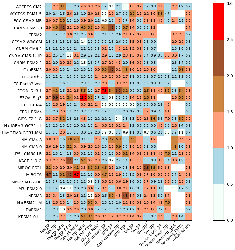
Figure 1Summary of RMSE values for the large-scale assessment criteria and regional temperature. The regions are abbreviated as follows: northern Europe (NEU), central Europe (CEU) and the Mediterranean (MED). Tas refers to near-surface air temperature, SPG refers to subpolar gyre, and UA and VA are the eastward and northward wind vectors at 850 hPa, respectively. The colour scale is determine by the ratio of the model RMSE to the ensemble mean RMSE. RMSE values are absolute, and the mean score is the average of the relative error (normalised by the ensemble mean) across each of the criteria.
3.2.1 Large-scale circulation patterns
The large-scale seasonal circulation pattern was assessed for winter (DJF) and summer (JJA) based on the mean climatology at 850 hPa for the baseline time period 1995–2014; the ERA 5 reanalysis was used for comparison (Fig. 2).
In DJF, European weather is dominated by the passage of weather systems that make up the NA storm track; the prevailing direction for these is from the southwest, as can be seen in the climatology in ERA5 (Fig. 2a). The model large-scale RMSEs for the 850 hPa wind vectors (e.g. Ashfaq et al., 2022; Chaudhuri et al., 2014) and a qualitative assessment of the overall circulation pattern were used to assess the models for this criterion. Figure 1 shows that the wind vector RMSE is less than that of the multi-model mean for CNRM-CM6-1 and HadGEM-GC31-LL. Where the wind vector errors for a model are less than the multi-model mean, the large-scale circulation is found to be reasonably well represented. Figure 2b and c show that these models capture the overall circulation pattern well and have relatively low wind speed biases. Where the models have a larger RMSE for wind vectors than the multi-model mean, the threshold for an unsatisfactory model requires some consideration. For these cases, a qualitative approach is used to understand how these errors may impact the European climate and to guide where this threshold should lie.
The model with the largest errors of the satisfactory models is CESM2, with an area of positive bias over the UK; however, this model was still assessed as satisfactory due to the well-defined southwesterly wind patterns and the good representation of the winds over most of the European land areas. The strength of the southwesterlies over the UK and Scandinavia is too weak in some of the models (e.g. IPSL-CM6A-LR; Fig. 2f), along with the prevailing wind direction being too westerly. These models were flagged as unsatisfactory. These models feature a variety of structural biases – for example, INM-CM4-8, which had a lower spatially averaged RMSE wind speed error but lacked a clear representation of the southwesterlies over northern Europe. The winds are too weak in these areas, and there are areas of negative bias in the Mediterranean. This model was classified as unsatisfactory due to its lack of representation of the circulation pattern and due to the general wind direction being too westerly (Fig. 2g). This is also reflected in the wind vector errors (Fig. 1).
Models flagged as inadequate have an almost entirely westerly (no southwesterlies) wind pattern, and the wind speed errors over large parts of Europe are widespread and substantial (e.g. CanESM5, FGOALS-g3; Fig. 2h–j). These models nearly all have a large (positive) bias over European land regions (e.g. > 6 m s−1). MIROC-ES2L has the largest errors for the wind vectors in the ensemble for DJF (more than twice the ensemble mean error for the eastward wind, UA); the errors do not follow the same pattern as the other inadequate models, with a large negative bias over most of Europe and an almost northerly wind direction in the NA (Fig. 2i).

Figure 2Examples of DJF circulation (850 hPa) classifications for a sample of individual models. Top panel shows ERA5 climatology. Wind speed and direction are shown as a 20-year mean (1995–2014). Arrows show the direction (absolute) of wind speed (scaled by wind speed) for climatology across all panels. The shading for the three panels shows the difference in wind speed between the model and ERA climatology.
Circulation patterns are more westerly with weaker winds in the summer (JJA). These were assessed using the same approach for comparison as for winter circulation (Fig. 3). Many CMIP6 models capture the general pattern well (e.g. HadGEM-GC31-LL, GFDL-ESM4; Fig. 3b and d). The UA and VA (northward wind) RMSEs for both of these models are less than the ensemble mean RMSE. Again, where the models perform above the average for the multi-model ensemble, the overall circulation pattern is well represented with relatively low wind speed bias. As with the case for the DJF circulation, where the models have larger errors than the multi-model mean for JJA wind vectors, the threshold is to warrant a flag as unsatisfactory or inadequate, as determined alongside some qualitative interpretation of the model errors.
Some of the models had westerly patterns over the UK and central Europe that were too weak (e.g. MIROC6, INM-CM4-8; Fig. 3f and h); as a result, there were larger errors in European land regions, and these models were therefore classified as unsatisfactory or, in the case of INM-CM4-8, where these errors are more pronounced, inadequate. In the case of MIROC6, we note that the magnitude of the UA and VA errors over the large-scale region assessed as a whole were on the borderline of the threshold between satisfactory and unsatisfactory compared to the other models. The relatively weak circulation and low bias in wind speed over the European land regions tare the reason for the unsatisfactory flag in this case (Fig. 3e).
The INM-CM4-8 (and, to a similar extent, the INM-CM5-0) model has some of the largest errors for the JJA wind vectors in the multi-model ensemble. It is noted that these models are also flagged as inadequate for both severe JJA blocking errors and severe errors in representing the annual precipitation cycle in central Europe. There are also issues with the temperature bias in central Europe for this model (flagged as inadequate). These severe errors in central Europe are likely to be related to the representation of the large-scale circulation.
For NorESM2-LM and ACCESS-ESM1-5 (Fig. 3i and j), the westerly pattern was too far north, leading to a large area of positive bias over northern Europe. These models have the largest RMSEs for wind vectors in the multi-model ensemble, along with the INM-CM4-8 and INM-CM5-0 models, and the largest RMSEs for wind speed. The large region of substantial positive bias over the NA and much of Europe indicates that this error is likely to have an impact on the JJA storm track over Europe for these models. As the storm track assessment is available for both these models, this can be confirmed to be the case. The storm track RMSE is in the top 85th percentile for the models assessed for the storm tracks (see the following section on the storm track assessment), and Fig. 1 shows that these models have the largest errors for the JJA storm track in the ensemble.
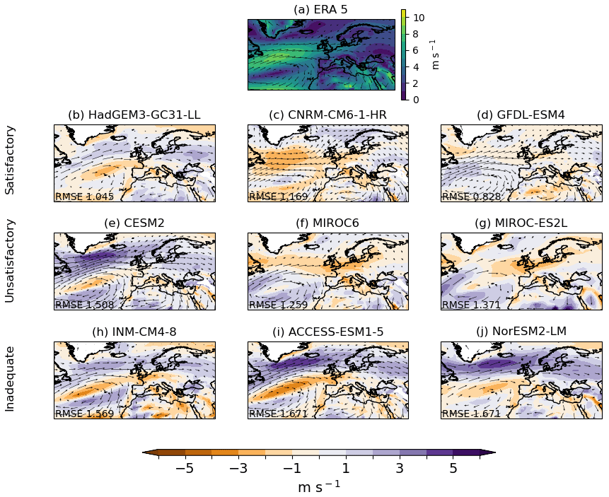
Figure 3Examples of JJA circulation (850 hPa) classifications for a sample of individual models. Top panel shows ERA5 climatology. Wind speed and direction are shown as a 20-year mean (1995–2014). Arrows show the direction (absolute) and wind speed (scaled by wind speed) for climatology across all panels. The shading for the three panels shows the difference in wind speed between the model and ERA climatology.
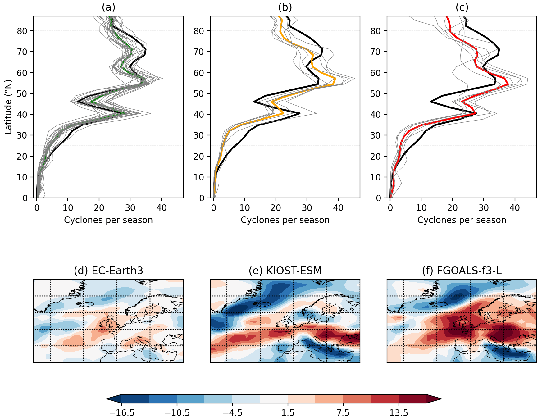
Figure 4Examples of DJF storm track classifications; (a), (b) and (c) show the RMSEs of the zonal mean track (20∘ W–20∘ E) for individual models and the classification mean for satisfactory (a), unsatisfactory (b) and inadequate (c). In (a)–(c), grey lines are the individual models, solid-coloured lines are the group average, and the solid black line is ERA5. Individual examples are shown in the lower panel for track density bias for satisfactory (d), unsatisfactory (e) and inadequate (f) models. Units of (d)–(f) are cyclones per season per 5∘ spherical cap.
3.2.2 Storm track large-scale assessment
The track density is calculated using an objective cyclone-tracking and identification method based on the 850 hPa relative vorticity (Hodges, 1994, 1995). The method and data are the same as those used in Priestley et al. (2020). The zonal mean of the model mean track density from 20∘ W to 20∘ E was taken to get a profile of storm number by latitude. Then, the RMSE of the models was calculated and compared to the profile obtained from ERA5. The RMSE was calculated from 25 to 80∘ N.
The storm track has been assessed as a large-scale feature using an assessment of the characteristic trimodal pattern (Fig. 4), calculated as the zonal mean of the seasonal track density between 25–80∘ N and 20∘ W–20∘ E compared to ERA5 reanalysis data. The baseline time period used for this assessment is 1979/1980–2013 (as in Priestley et al., 2020). The RMSE of the zonal mean track density from 20∘ W to 20∘ E is used to initially sort the models into categories; while a hard cutoff threshold was not applied for each category, it was helpful to sort the models into <65th, 65th, 85th and >85th percentiles for RMSE. The different model groups were then inspected visually, and it was found that, although some of the models in the <65th percentile had some significant biases, the models in this group had clearly defined peaks in their number of cyclones at the correct latitude and therefore captured the passage of storms across western and central Europe satisfactorily (Fig. 4a). This was not found to be the case for the models in the 65th–85th RMSE percentiles, where there was a lack of a northern peak; this indicates a zonal bias in these models, which is a characteristic bias in GCMs (Fig. 4b). These models were classed as unsatisfactory; the errors were not large enough on visual inspection to class them as inadequate, with the exception of MIROC-ES2L.
Models with >85th percentile RMSEs failed to capture the trimodal pattern and had large biases in the number of cyclones at each of the peaks (Fig. 4c). In particular, there was a lack of a northern peak and an amplification of the errors in this group, with a large zonal bias in the track density. These models were considered to be unable to represent this feature and were flagged as inadequate. Examples of individual models for each of the groups are shown in Fig. 4d–f. The RMSE values for each of the models in the multi-model ensemble are also shown in Fig. 1.
3.3 Weighting for performance against global trends and model independence with the ClimWIP method
We also compare our results with the Climate model Weighting by Independence and Performance (ClimWIP) method (Knutti et al., 2017; Lorenz et al., 2018; Brunner et al., 2019, 2020b; Merrifield et al., 2020) to assess differences between our process-based filtering and an assessment based on historical warming. ClimWIP combines model performance weighting based on one or more metrics with an assessment of model independence (i.e. overlaps in the models' source code or development history). Here, we use an adaptation of the approach described in Brunner et al. (2020b) and publicly available via the ESMValTool (https://docs.esmvaltool.org/en/latest/recipes/recipe_climwip.html, last access: 14 April 2023). Performance weights are calculated based on global temperature trends compared to ERA5 for the period 1980–2014. Independence weights are based on global model output fields for temperature and sea-level pressure, which have been shown to reliably identify model dependencies (Brunner et al., 2020b; Merrifield et al., 2020). Here, we use ClimWIP in two setups: one only based on performance weights and one only based on independence weights, as detailed later.
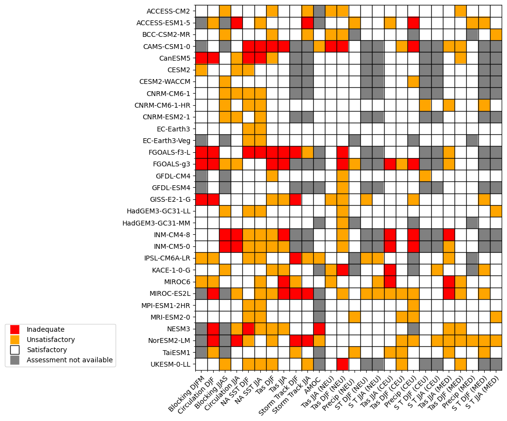
Figure 5Model assessment summary for qualitative European criteria. Assessment criteria for the large scale are as follows: blocking – blocking frequency; circulation – large-scale circulation assessed by 850 hPa wind speed and direction; NA SST – NA SST bias; Tas – surface air temperature bias at 2 m; storm track – based on RMSE of the zonal mean track 20∘ W–20∘ E; and AMOC – based on strength at 1000 m at 26∘ N. Assessment criteria for the European regions are as follows: Tas – surface air temperature bias at 2 m; Precip – annual precipitation cycle; and ST – storm track assessed as cyclones per season within the European region.
4.1 Assessment table
The assessments for each of the CMIP6 models are collated into Fig. 5, with the classification for each of the criteria, where the relevant data and/or analyses are available. Figure 5 creates a summary of each model's performance against a range of criteria that are essential for a meaningful representation of the European climate. This summarises the skill, across a multi-model ensemble from CMIP6, in terms of their ability to capture the key processes for the European climate. The assessment criteria are divided into large-scale and regional assessments. The large-scale assessment criteria, such as large-scale circulation and blocking frequency, are criteria that have a pan-European impact and are not specific to a particular region. The regional assessment criteria have been scored individually for each of the three main European regions used in the EUCP study and as defined in Brunner et al. (2020a) and Gutiérrez et al. (2021). These are, northern Europe (NEU), western and central Europe (CEU), and the Mediterranean (MED; see Fig. S1 in the Supplement). We focus in the assessment on summer (JJA) and winter (DJF).
Some of the criteria were assessed both at the large scale and regionally. For example, it is useful to know if a model has a widespread temperature bias that extends over Europe and the NA, but it is also the case that some models have more localised temperature biases that affect individual regions. For the regional assessment where surface variables (e.g. precipitation and temperature) are assessed, models were scored for their performance solely over the land regions.
The classifications in Fig. 5 can be applied to create a bespoke subset of CMIP6 models depending on the motivation for sub-selecting. Here, we have used the red classification of inadequate to indicate that a model should be removed, but it may be the case that a less strict approach to performance filtering than what we have applied here would be acceptable in some cases. Likewise, it may be the case that an unsatisfactory (orange) flag for a certain criterion, such as the regional precipitation, may be particularly undesirable. In the following section, we use the table to create two different subsets from the multi-model ensemble.
4.2 Excluding the models least representative of key regional processes
In this section, we explore the implications of screening out poor models based on the process-based performance assessment alone for the range of projected regional changes. The aim is to revisit the range of projected regional climate changes, excluding those shown to struggle with representing regionally relevant processes. Note that, for this reason, we do not include in this section any criteria based on climate sensitivity or global temperature trends. These additional considerations and how they could be applied will be discussed along with the results.
For the sub-selection process, we refer back to the definition of the classifications in Sect. 2.2. The inadequate category (shown as a red flag in Fig. 5) is used to indicate that a model fails to represent a key feature of the regional climate and should be removed from the sub-selection. We also differentiate between large-scale criteria that can be expected to have pan-European effects on the model performance (and may also be inherited from the GCM in case of down-scaling) and regional criteria that may only be of concern in the local region. Here, we consider the impact on the projection range of excluding any model with one or more inadequate (red) flags for any of the large-scale criteria. We then go on to consider any further changes in the projected temperature range as a result of removing any remaining models with a regional inadequate flag.
Once all the models in Fig. 5 that have a red flag for the large-scale criteria are removed, the following models remain in the sub-selection: ACCESS-CM2, BCC-CSM2-MR, CESM2, CESM2-WACCM, CNRM-CM6-1, CNRM-CM6-1-HR, CNRM-ESM2-1, EC-Earth3, EC-Earth3-Veg, GFDL-CM4, GFDL-ESM4, HadGEM3-GC31-LL, HadGEM-GC31-MM, MPI-ESM1-2-HR, MRI-ESM2-0, KACE-1-0-G, TaiEMS1 and UKESM1-0-LL. This sub-selection from the qualitative assessment can also be compared to the RMSE values in Fig. 1. If we look at the scores for the large-scale criteria (all categories in Fig. 1, excluding regional temperature), it can be seen that the excluded models include all those with an RMSE more than 1.5 times the ensemble mean in at least one of the large-scale categories. It is also the case that, for the retained models, the RMSE does not exceed 1.5 times the multi-model ensemble mean for any large-scale category. The retained models also perform better than or are at least equal to the ensemble mean across all the categories. This indicates that, in our application of the assessment, objectively poorer models have been removed (in terms of large-scale performance), and those with objectively smaller errors have been retained.
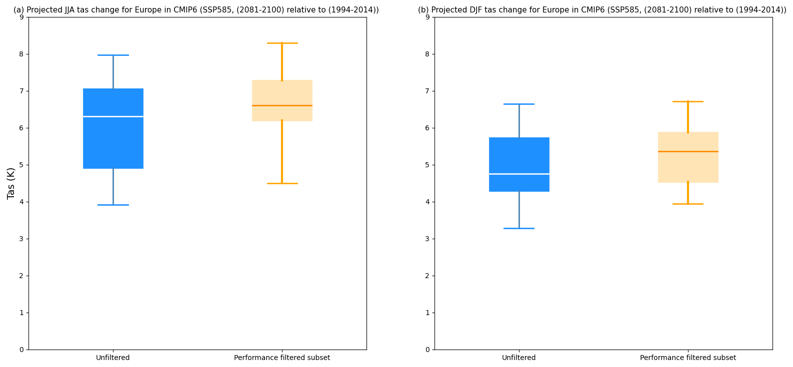
Figure 6(a) Projected range of JJA temperature change for Europe in CMIP6 (SSP585; 2081–2100 relative to 1994–2014) for the raw unweighted multi-model ensemble and the large-scale performance-filtered subset. Boxes show the 25th to 75th percentiles. Whiskers show the 5th and 95th percentiles. (b) As for (a) but for DJF.
Figure 6 shows the difference in the projected temperature range for the large-scale process-based filtered subset and the unfiltered multi-model ensemble. The difference in DJF is small (Fig. 6b); however, in JJA, the lower part of the range is reduced, and the upper part is shifted upwards (Fig. 6a). This shift in the projection range indicates that more of the higher-sensitivity models are retained by filtering using process-based performance criteria.
In the second stage of filtering, we again refer to the regional criteria in the assessment table. There are inadequate (red) flags for regional precipitation (in central Europe) and for regional temperature in a few of the models (Fig. 5). The models with an inadequate classification for precipitation (INM-CM4-8, INM-CM5-0, ACCESS-ESM1-5 and FGOALS-g3) already have at least one inadequate flag for the large-scale atmospheric criteria. Therefore, these models have already been removed from the performance-filtered subset. The KACE-1-0-G model has two inadequate flags for regional temperature in two regions, namely NEU and CEU. The UKESM1-0-LL model has a single inadequate (red) flag for temperature in DJF (NEU). Figure 1 shows these temperature errors in both models to be relatively large compared to the multi-model-ensemble mean RMSE. In addition, the UKESM1-0-LL model has a relatively large DJF temperature error for CEU, indicating that this temperature bias extends over two of the European land regions. These errors that are limited to specific regions may be considered acceptable for some applications, and so there may not necessarily always be a reason to exclude a model from a sub-selection. Here, we filter the subset further by removing these models. Referring to Fig. 1, we can confirm that our excluded models include only those with a relatively large RMSE (1.5 times the ensemble mean) in at least one of the criteria and that the eliminated models, on average across the criteria, have a relative error at least equal to or larger than the ensemble mean (Fig. 1). Therefore, it is again the case that the qualitative assessment has removed the models with objectively larger errors in the key criteria.

Figure 7(a) Projected range of JJA temperature change for Europe in CMIP6 (SSP585; 2081–2100 relative to 1994–2014) for the raw unweighted multi-model ensemble, the performance-filtered subset and the raw ensemble weighted for performance against global trends using the ClimWIP method. Boxes show the 25th to 75th percentiles. Whiskers show the 5th and 95th percentiles. (b) CMIP6 model ECS compared to consolidated regional performance index. The yellow bounds show the IPCC AR6 likely range for ECS; the grey bounds show the very-likely range.
Figure 7a shows the difference in the range of projected temperature in the large-scale and regional performance-filtered subsets compared to the raw unweighted ensemble for JJA. In comparison, the shift in the projected range for DJF is small (Fig. S2). The lower part of the range is substantially reduced for the processes that are performance filtered in JJA (Fig. 7a).
The filtered subset of models retains more of the models with higher sensitivity; this contrasts with the existing literature regarding observational constraints on regional climate projections in CMIP6. There is existing literature that has used the ability of CMIP6 to capture either regional temperature trends (e.g. Ribes et al., 2022) or global trends (Liang et al., 2020; Ribes et al., 2021; Tokarska et al., 2020; Brunner et al., 2020b) that down-weight models with larger climate sensitivities in favour of models with more modest climate sensitivities. We illustrate the contrast between this existing literature and our results by using the methodology of Brunner et al. (2020b) to illustrate the typical constraint on projections indicated in this literature. We use the method of Brunner et al. (2020b) (see Sect. 3.3), applying it to the global temperature trends to calculate performance weights for each model using the first ensemble member. These weightings shift the projected temperature range downwards compared to the unweighted raw ensemble (Fig. 7a). Our emergent relationship between less robust regional projections and lower-sensitivity models was unexpected and represents an apparent tension with the existing observational-constraint literature based on temperature trends.
A regional consolidated performance index was created by giving the satisfactory (white), unsatisfactory (orange) and inadequate (red) flags a numerical score of 1 for satisfactory, 2 for unsatisfactory and 3 for inadequate. The overall score for each model was then averaged by the total number of assessed criteria to give an indication of how the model performed overall. Many of the models that performed well for the process-based criteria do not fall within the IPCC AR6 likely range for equilibrium climate sensitivity (ECS; Forster et al., 2021; Fig. 7b).
Our result does not include any consideration of climate sensitivity, and while these models are identified here as performing relatively well in a process-based assessment, the subset temperature range shown in Fig. 7 should not be viewed as a constraint that gives a more accurate projected range for Europe. Here, we only highlight that more of the models that perform well in terms of regional physical processes have a higher climate sensitivity. It may be appropriate to select only the better-performing models from within the very-likely IPCC range for ECS or to retain just one of the models above this range to account for a higher-impact scenario. It may also be appropriate to select models that are marginal from the lower part of the IPCC very-likely range. Alternatively, using an approach that considers regional impacts using global warming levels could be applied to the subset; this is discussed further in Sect. 5.
4.3 Sub-selection for performance and model diversity
In this section, we consider how a sub-selection of a small number of example models that represent the broader characteristics of the wider filtered projection spread could be carried out. In this example application, we look for a subset of GCMs that are both in our filtered subset and sample this spread. The motivating criterion is the identification of models that perform well across the whole European domain and retain as much of the spread of future projections as possible. Such an approach might be adopted by those looking for a smaller subset to drive downstream models – for example, as a selection tool for a potential regional climate model (RCM) matrix, as data for a pan-European assessment of food security or for any other impact needing pan-European physically coherent climate projections, where the GCMs would then provide the climate-driving data.
The models from the process performance subset are placed into clusters of models that had clear dependencies (Table 1). The Euclidean distance of the models is determined using the ClimWIP method (see Sect. 3.3) for the comparison of model independence (Brunner et al., 2020b). Fig.S3 shows the independence matrix for the different models, which was used to create clusters of models that had dependencies. Models with a Euclidean distance of ≦ 0.6 were combined into clusters. Three models were found not to have a sufficient dependency in relation to the other models to be placed in any cluster (see Table 1). In most cases, many of the models with similarities were from the same institution or were known to share significant code components, such as the same atmosphere model in the HadGEM-GC-3.1 and ACCESS-CM2 models.
In this application, to maintain model diversity as far as possible, one model was selected from each of the clusters (and two from models that fell into no cluster). Using Fig. S4 to determine where the models are situated in the projected temperature and precipitation range for each region, these individual models are also selected to include as much of the temperature and precipitation range of the filtered multi-model ensemble as possible. The selection chosen for this example is illustrative, and it may be appropriate to sub-select differently depending on the intended application of the sub-selection. The selected models for this example are shown in blue (Fig. 8).
In this section, we have shown one example of sub-selection of a smaller subset using the filtered models from the previous section. There are a number of different smaller subsets that could be selected using the information from the assessment tables (Fig. 5). Depending on the intended application of the sub-selection, a different approach (for example, one that includes plausible outliers – e.g. models that do not have red flags in large-scale criteria) may be more appropriate in order to sample high-impact, low-probability regional responses.
Table 1Table showing models clustered based on Euclidean distance.
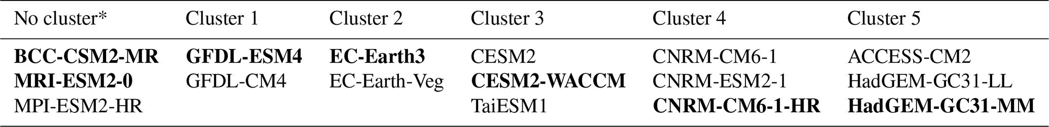
* Models were not found to have sufficient dependencies to be placed in a cluster. Selected models are shown in bold.
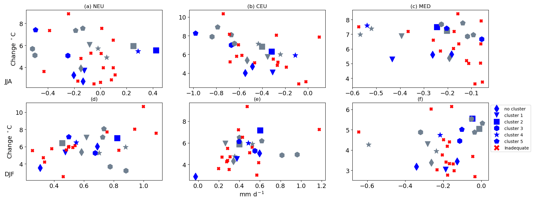
Figure 8Temperature and precipitation projection range (SSP585; 2018–2100 relative to 1995–2014) for CMIP6 multi-model ensemble. Excluded models are shown in red. Models selected from each of the seven clusters in Table 1 are shown in blue. Models from the process-performance-filtered subset that were not selected are shown in grey. Models from the same cluster are indicated by symbols.
An overall aim of this study is to provide an assessment of CMIP6 models that can be applied by users that wish to create filtered subsets for Europe for a range of applications and that also wish to remove the least-representative models. The assessment information could be applied to a filtering approach that is tailored according to the criteria of interest. The assessment used in this study combines a qualitative and quantitative approach. To some extent, there is always a degree of subjectivity when grading models for performance; even where more objective techniques are used, such as clustering based on evaluation statistics (e.g. seasonal RMSE, correlation, bias as used for the blocking frequency here), there is still the difficulty of identifying where the thresholds for satisfactory or inadequate models should lie in addition to the assessment of the relative importance of one metric versus another (Knutti, 2010). The assessment of a satisfactory model will also inevitably be relative to the performance of other models in the ensemble. In the approach shown here, where the quantitative thresholds were used to guide the model classifications, these thresholds were largely determined according to the distribution of performance for the ensemble. It has also been an aim throughout to maintain consistency in the way that the classifications are applied for each of the assessment criteria. In practice, this can be difficult to achieve due to the fact that, for each criterion, many of the GCMs generally capture some of the large-scale processes (e.g. blocking frequency and CEU precipitation) relatively poorly in comparison to others, while other criteria (e.g. AMOC) can be difficult to evaluate.
A further challenge is that not all models have been assessed against all criteria. Analyses that assessed storm tracks, blocking frequency and the AMOC provide valuable further information regarding the performance of the models but were not available for every model in the study; therefore, it was necessary to consider whether a model should be eliminated on the basis of one of these criteria when other models, whose performance was unknown, may have been kept in the selection. It was found to be the case that the flags for exclusion did not occur in isolation. Severe errors (red flags) for large-scale circulation, storm tracks and blocking frequency often occurred in more than one criterion (or, in some cases, alongside multiple orange flags). Severe errors (or inadequate flags – i.e. those flagged red) in the AMOC, another criterion where data were limited, were due to a very weak representation of this feature, and where this was the case, a severe cold bias in the SPG region was also present (NESM3).
Considering the regional impact of eliminating the models flagged as inadequate (flagged red; Fig. 5), the lowest temperature response models are excluded in summer (JJA) for the NEU, CEU and MED (Fig. 8). For summer rainfall, in the NEU and MED, many of the models showing a more neutral change in rainfall are excluded. Greater warming is generally linked to stronger summer drying and increased winter precipitation. The exclusion of many of the models with a more modest projected temperature increase also results in the exclusion of many of the models with more neutral projected changes in precipitation.
Filtering of the CMIP6 ensemble by excluding the least-realistic models for Europe leads to the removal of models throughout the projected temperature range but particularly models that have a more modest response. The retention of higher-sensitivity models is due to more of the higher-sensitivity models demonstrating a greater skill in reproducing regional processes. The revised temperature projections for the filtered GCMs for each region lead to a shift upwards in the median of the projected JJA temperature range due to more of the higher-sensitivity models performing well against the process-based criteria (Fig. 7). This may represent a particular challenge for potential applications where sampling regional climate responses in the lower end of the IPCC climate sensitivity (ECS) range is required, as many of the CMIP6 models in the lower part of the ECS likely range were excluded by our processed-based assessment (Fig. 7b). Using the IPCC AR6 likely range for ECS (and for TCR; Hausfather et al., 2022) has also been suggested as an approach to model screening for the CMIP6 ensemble. Other regional sub-selection studies for CMIP6 have eliminated models with high global sensitivity (Mahony et al., 2022). Any assessment that excludes models based on both the performance criteria here and metrics like global climate sensitivity or global trend criteria (which tend to exclude models with higher climate sensitivities) will be left with only a small subset of adequate models. This apparent tension is likely to be less evident where global warming levels are instead adopted. Using this approach when adopting a selection based on climate performance, such as that presented here, would enable the exploration of a broader set of adequate realisations.
Our results contrast with the existing literature in terms of evaluation against historical temperature trends (Liang et al., 2020; Ribes et al., 2021; Tokarska et al., 2020). Many of the models that score well against process-based criteria have a higher ECS. ECS is not considered in this study as a sub-selection criterion because the focus of this work was on the assessment of how well models capture the main regional climate processes. Links between the plausibility of CMIP6 projections, based either on their historical global or regional temperature trends or climate sensitivity (Hausfather et al., 2022), are well established in the literature for CMIP6 (Ribes et al., 2021; Liang et al., 2020; Tokarska et al., 2020). When the raw ensemble is weighted against performance for global trends (Fig. 7a), the effect is to shift the temperature range downwards. This shift for our raw ensemble is not as large as that typically seen in other studies for global trends (e.g. Liang et al., 2020; Ribes et al., 2021; Tokarska et al., 2020). This may be due to our use of a single ensemble member for this study, some differences in methodology or summer warming in Europe being thought to be about 30 % higher than the annual mean global warming (Ribes et al., 2022).
Ribes et al. (2022) find a constrained regional projection range for mainland France for ssp585 (5.2 to 8.2∘) that is similar to the projected range of our performance-filtered subset for summer using a combination of modelling results and observations. Our upper 95th percentile and lower 5th percentile are a little lower than this (for a pan-European range); our median for the performance-filtered range is very similar to their central estimate of 6.7 ∘C (Fig. 7a). For assessments of model performance against historical temperature trends, where the regional trends are also taken into account, there may be less of a tension with our assessment than is the case with those that are based on global trends alone (e.g. Liang et al., 2020; Ribes et al., 2021).
We provide an assessment of regional processes and biases (Fig. 5) for a multi-model ensemble from CMIP6 that can be used to inform sub-selection for the European region. This can be used to aid the creation of bespoke sub-selections for a particular application (e.g. sub-selection of a small number of representative ensemble members for downscaling or impact assessments); alternatively, the subsets that have been demonstrated here can be also be used directly.
Filtering an ensemble of CMIP6 models based on performance in terms of key process-based criteria results in the projected temperature range being shifted upwards. This is due to the removal of a larger proportion of the lower-climate-sensitivity models that do not perform adequately against the assessment criteria. We also find that many of the higher-sensitivity models score well against the process-based assessment and that these models are better able to represent the features of the European climate. It is not clear whether the emergent relationships we found (between better models and higher sensitivities) are circumstantial or reflect an underlying physical basis. If they reflect an underlying physical relationship (where atmospheric processes needed to capture regional feedbacks also drive stronger climate feedbacks), then this might imply greater confidence in higher-end regional changes. If, on the other hand, the sampling of higher-sensitivity models is circumstantial (simply due to chance), this represents a challenge, as there are few CMIP6 models that sample the central and lower end of the IPCC AR6 likely climate sensitivity range. This remains an open question, which we have not been able to resolve in this work.
Our results highlight a tension in terms of regional sub-selection between performance measured against the global temperature trend and the ability of the models to capture the features of the regional climate in the CMIP6 multi-model ensemble. For cases where changes in temperature are not the only variable of interest (or the primary concern), many of the higher-sensitivity models are likely to provide more reliable information regarding the future climate. Potential users of regional climate projections should be aware that there is a potential tension between constraints from large-scale temperature change or climate sensitivity and the assessment of regional processes, at least for Europe.
A1 Annual precipitation cycle
The annual precipitation cycle was assessed as a regional criterion for each of the European land regions (Gutiérrez et al., 2021; see Fig. S1). The precipitation cycle for each model was assessed against the E-OBS (Cornes et al., 2018) data as monthly means (see Fig. A1) using the baseline period of 1995–2014. A combination of the correlation and RMSEs for each of the four seasons is used to assess whether models should be categorised as either satisfactory or unsatisfactory.
In order to sort the models into categories, the seasonal RMSE and correlation were used as a guide (Fig. A1b–e). It was observed that, in most regions, a poor correlation with the observed cycle had a large seasonal RMSE compared to other models (>0.75 mm d−1) in at least one season. The exception was in CEU, where most models had a poor correlation with the observations. The models with a relatively low error of less than 0.6 mm d−1 for all four seasons were classified as satisfactory. Models with an RMSE greater than 0.75 mm d−1 in one season were classified as unsatisfactory.
In CEU, the models with a substantially negative correlation (approx. −0.25) had a large seasonal RMSE (> 1 mm d−1) and very poor agreement with the seasonal cycle, where they essentially showed a strong seasonal drying in the wet season for CEU (Fig. A1). These models are classified as excluded.
There were some models (RMSE >0.6 mm d−1 <0.74 mm d−1) that did not fall immediately into any classification. Where the RMSE error in all seasons was ≪0.74 mm d−1, the model performance was generally satisfactory. However, in the case of some models closer to this threshold, a lower correlation with the E-OBS data rendered them unsatisfactory.
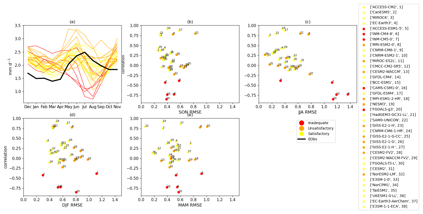
Figure A1Precipitation annual cycle for CEU (a); model comparison with E-OBS (shown as solid black line). Correlation (over 12 months) and seasonal RMSEs for each model. Monthly averages are taken over a 20-year climatology (1995–2014). The RMSEs and correlations are calculated from the monthly averages.
A2 Sea surface temperature bias
Seasonal average sea surface temperatures (SSTs) were assessed for each of the models using the HadISST1 (Rayner et al., 2003) reanalysis (Fig. A2) for the baseline period 1995–2014. Surface skin temperatures from the atmospheric models were used; the corresponding ice concentration fields from the atmosphere model were only available for a smaller number of models. To estimate the ice extent and to avoid errors in the assessment of the SST bias in areas affected by ice, a seasonal average TS < 0 ∘C is used as a proxy for the 5 % ice concentration to mask these areas. The areas masked by this proxy are compared to the extent of the 5 % ice concentration in the models and are found to be a good approximation. As the area affected by ice is approximated, this is not compared directly to the 5 % ice field from HadISST1 for the assessment; however, where the masked areas are significantly larger than the 5 % ice concentration in HadISST1 (Fig. A2, bottom right), a large cold bias in these areas is inferred (Fig. A2). This bias in sea ice and the SST surrounding northern Europe is found to be well captured by the large-scale near-surface temperature bias (see Sect. A3). Therefore, it is noted here as an important consideration for the European climate, but it is not included explicitly in the assessment of the NA SST error classifications. For the NA SST assessment, we focus on errors in key regions of the NA for the European climate.
The NA SST assessment is based on two key areas of the NA, the subpolar gyre (SPG) and the Gulf Stream northwest corner (GS) regions. These have been selected from Ossó et al. (2020), who identified a northwestern region of the North Atlantic GS as important for weather patterns over Europe, and from Borchert et al. (2021b) to define the SPG region, which has previously been shown to modulate the probability of the occurrence of summer temperature extremes in central Europe (Borchert et al., 2019; Fig. S7). These regions, as well as their gradients, have been demonstrated to carry relevance for the dynamical atmospheric influences of NA SST on European summer climate (Carvalho-Oliveira et al., 2022), highlighting their relevance in the context of this study. During a qualitative inspection of the models (see Fig. A2), these regions were also identified as areas that routinely show a substantial bias in the models.
A small number of models had extensive areas with a very large winter negative SST bias (Fig. A2, bottom row); this results in a substantial overestimation of winter ice extent to the north of Scandinavia and around Greenland. NESM3 and CAMS-CSM1-0 had a large, widespread negative bias that extended beyond the regions of sea ice to the NA and SPG (Fig. A2). The models with the largest SPG RMSE are NESM3, CanESM5, CAMS-CSM1-0 (shown in Fig. 1) and FGOALS-f3-L. In addition, FGOALS-f3-L has an RMSE for the GS region of more than 2 times the ensemble mean RMSE. These models are all flagged as inadequate.
A number of models also had areas with substantial but limited areas of warm bias (>6 K) in the area around the Gulf Stream and larger areas in the SPG (>3 K), e.g. CESM2, INM-CM50 and NorESM2-LM (Fig. A2). In addition, these models also had areas with cold bias in the SPG. This combination of warm and cold biases in different areas also results in a poor representation of the SPG temperature gradient. These models also had an RMSE larger than that of the ensemble mean in the SPG assessment region and were classified as unsatisfactory. The INM models are an exception in the unsatisfactory category in terms of not having a large SPG error; however, these two models have some of the largest errors in the GS region, with the exception of FGOALS-f3-L.
Satisfactory models had a lower bias in all areas. Some had small areas with a larger bias (often around the Gulf Stream or in some parts of the SPG, e.g. ACCESS-CM2), but the effect of these areas did not prevent a reasonable representation of the SPG gradient. The models classified as satisfactory all have an RMSE in the assessed region that is less than the ensemble mean.
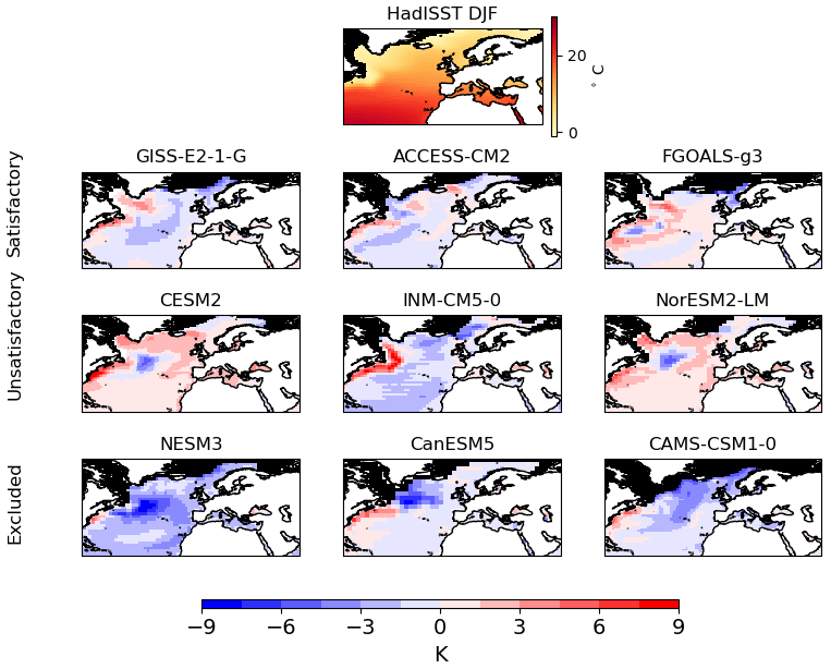
Figure A2Model SST bias (compared to HadISST) for DJF. Seasonal average calculated for a 20-year climatology (1995–2014). Areas where the model SST <0 ∘C are masked in black (this was found to approximate 5 % ice concentration). Top row shows the HadISST and 5 % ice concentration field.
In JJA, the satisfactory models again had smaller areas of bias (>3 K) around coastal regions, but these were not widespread (Fig. A3). Models flagged as satisfactory also had SST RMSE in the SPG and GS regions that were less than the ensemble mean error. Although the model errors in the SPG and GS are satisfactory, there is a cold bias in the SSTs in the Norwegian and Barents seas in the FGOALS-g3 (and GISS-E2-1-G) model. In the FGOALS-g3 model, there is also an excess in the sea ice extent in the Barents region. While the SST assessment has been focused on the NA SST region, it is noted that biases in this region are also important for the European climate. These biases are captured in the model classification for temperature bias (which includes near-surface temperature bias over the ocean).
The unsatisfactory models had larger regions with a substantial cold bias in the SPG and/or larger biases in the GS region that were larger than the ensemble mean. The CAMS-CSM1-0, CanESM5 and FGOALS-f3-L models with the largest SPG errors were classed as inadequate.
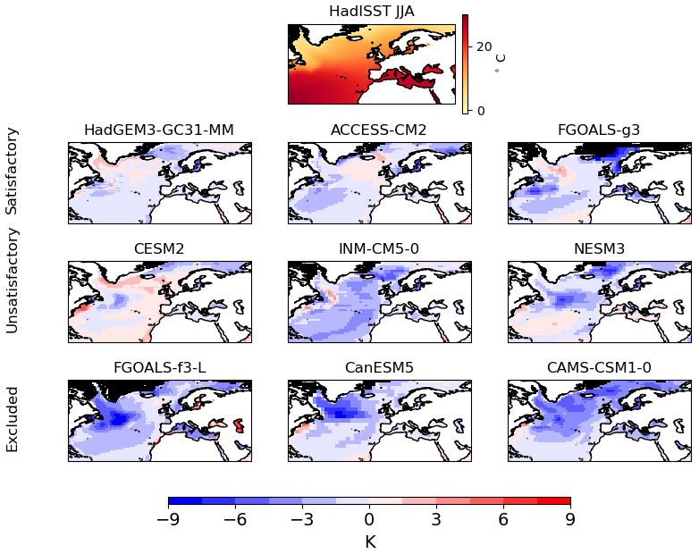
Figure A3Model SST bias (compared to HadISST) for JJA. Seasonal average calculated for a 20-year climatology (1995–2014). Areas where the model SST <0 ∘C are masked in black (this was found to approximate 5 % ice concentration). Top row shows the HadISST and 5 % ice concentration field.
A3 Near-surface temperature bias
A3.1 Large-scale bias
The model near-surface temperatures are compared to ERA5 reanalysis (Fig. A4) for the baseline period 1995–2014. These were assessed for the large-scale domain (including surrounding areas over the NA, Norwegian Sea, Barents Sea and nearby Arctic regions) criteria (Fig. A4) and also, more specifically, for the land points of each SREX (Special Report on Managing the Risks of Extreme Events and Disasters to Advance Climate Change Adaptation) region (see Sect. A3.2).
For the large-scale assessment, there is inevitably some overlap with the assessment of SST temperatures, as near-surface temperature over North Atlantic regions is taken into account. The large-scale qualitative assessment considers whether there are widespread areas of temperature bias in land regions of Europe or in other regions where they could be expected to have downstream impacts, e.g. nearby land areas in the NA or other ocean regions nearby the European land areas. A more widespread bias as opposed to a smaller, more regionally based temperature bias indicates an issue with the large-scale processes that will affect all the European regions, while a more local area of bias is likely to indicate issues related to processes in a particular region. Where biases in land regions are found in more than one European region, however, these are likely to also indicate an issue that may affect the whole European area. The RMSE over the region as a whole and over each of the land regions is taken into consideration for the model calculation alone, with a more qualitative assessment of regions of bias.
For JJA, MIROC6 has a large, widespread positive summer bias over European land regions, north Africa and Greenland. This bias is largest in the CEU and MED, but this is not extended over the NA, where there is a cool bias. The warm bias in the MED and CEU regions is exceptionally large (>8 K in some areas), but it is not limited to these regions, with a smaller but still-substantial bias for all land regions (Fig. A4). The RMSE is the largest in the model ensemble for the whole region and for the northern and central regions. MIROC-ES2L has a similar pattern of errors as MIROC6 (although not quite as large, it is still more than 1.5 times the ensemble mean RMSE). CAMS-CSM1-0 has a large, widespread negative bias in all areas of Europe; this model also has a large cold bias in JJA for both land and SST. It has one of the largest RMSEs for the large-scale region and the largest in the ensemble for northern Europe. FGOALS-g3 also had widespread biases, with an unusual pattern showing an area of exceptionally large cold bias to the north of Scandinavia and the UK (>8 K), while also having a substantial warm bias in the eastern area of CEU (4–6 K around the Black Sea area). The RMSE for the whole region is above average but not exceptionally large compared to the rest of the ensemble. This is largely due to a relatively small bias in the NA, as noted in the SST assessment. The RMSE error in the central European region is more than 1.5 times the ensemble mean. The additional area of large low bias in the areas of the Norwegian and Barents seas, with the resulting excessive sea ice (see Fig. A3), has led to this model also being rated as inadequate. The INM-CM4-8 model has a large positive bias in both the central and Mediterranean regions, and the RMSE for both these regions and the SPG is more than 1.5 times the ensemble mean error; therefore, this model has also been classified as inadequate.
Examples of models classified as unsatisfactory in terms of JJA bias include NESM3, GISS-E2-1-G and INM-CM4-8 (Fig. A4). NESM3 has a substantial warm bias in eastern CEU and MED regions (> 4 in some areas) and areas of cold bias in the NA (4–7 K). GISS-E2-1-G has substantially more widespread areas of cold bias (Fig. A4). The INM-CM5-0 model has a substantial warm bias in the central European region and SPG area. Its overall RMSE for the large-scale area is larger than the ensemble mean RMSE. This model is classified as unsatisfactory.
Examples of satisfactory models with a bias of ≦2 K in most regions and up to 4 K in limited regions for JJA include GFDL-CM4, CNRM-CM6-1-HR and EC-Earth3 (Fig. A4, top row). Models classified as satisfactory had large-scale RMSEs that were less than or close to (slightly above) the ensemble mean RMSE.
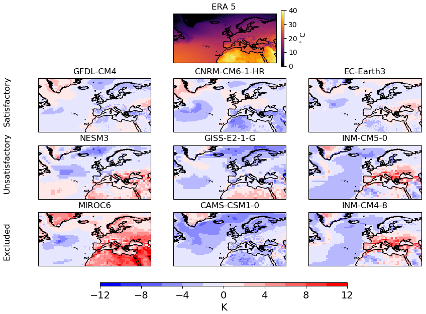
Figure A4Model temperature bias for the large-scale domain. Seasonal JJA average calculated for a 20-year climatology (1995–2014).
For DJF, the cold bias in the models that are classified as inadequate is pronounced, especially in northern European areas (Fig. A5). These models all had an RMSE for the large-scale area that was more than 1.5 times the ensemble mean RMSE. In the case of FGOALS-g3, it was more than 2 times the ensemble mean error.
The unsatisfactory models included those with a substantial cold bias in areas that, while not directly over European land regions, can be expected to have some downstream impacts on them (e.g. NESM3 and GISS-E2-1-G). In several cases, substantial biases are present in the land regions of interest (e.g. NorESM2-LM). The models classified as unsatisfactory all had RMSE errors large than that of the multi-model mean. The only exception is the UKESM1-0-LL, which had an RMSE for the large-scale area that was slightly lower but also had substantial errors in two European land regions (northern and central Europe) that were among the largest in the multi-model ensemble. Satisfactory models had smaller biases over all regions and an RMSE for the large scale that was smaller than that of the multi-model ensemble mean.
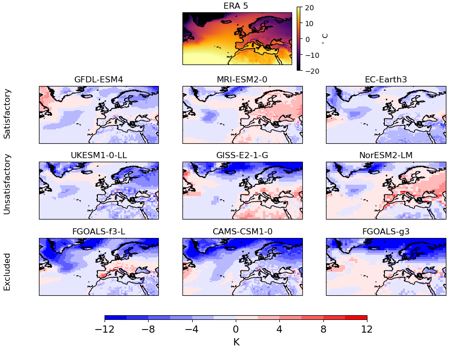
Figure A5Model large-scale temperature bias for the large-scale domain. Seasonal DJF average calculated for a 20-year climatology (1995–2014).
A3.2 European land regions
In addition to the large-scale assessment, the three IPCC AR6 land regions (Gutiérrez et al., 2021) were individually assessed to identify land areas of seasonal temperature bias. The spatial mean seasonal RMSE for all land points in each region was calculated and used as a guide for assessment along with a visual inspection of the spatial temperature bias. A small number of models were classified as inadequate for individual regions due to areas with a large local bias that were not excluded due to a temperature bias in the large-scale assessment. These models may be considered inadequate only for the region.
The RMSE for each region is used to classify the models. For JJA, the thresholds were <2.5 K for satisfactory, >2.5 K but <4 K for unsatisfactory and >4 K for inadequate. As is the case in determining any threshold, there is a degree of subjectivity, and these thresholds are based on the relative performance of the models across the ensemble. For DJF, the thresholds were the same, except that the threshold for inadequate was increased to >5 K.
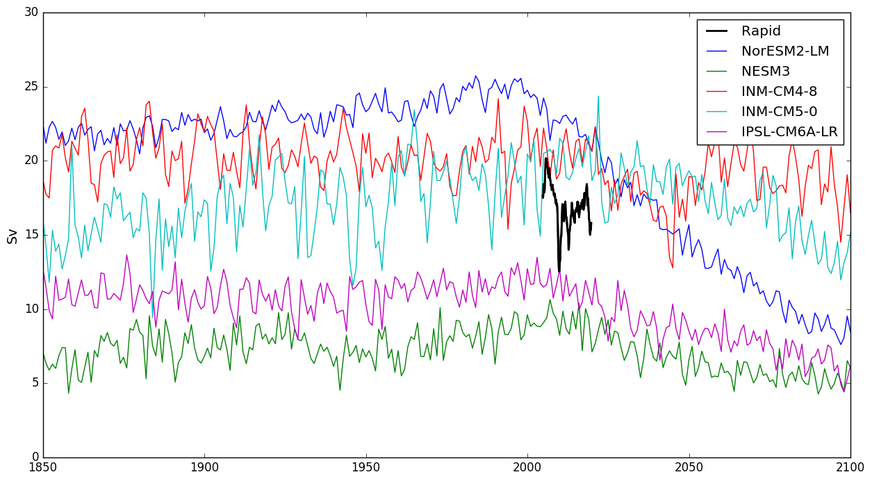
Figure A6AMOC strength at 1000 m (from v (velocities) compared to rapid array (annual mean Sv)) at 26∘ N. AMOC data are from Menary et al. (2020).
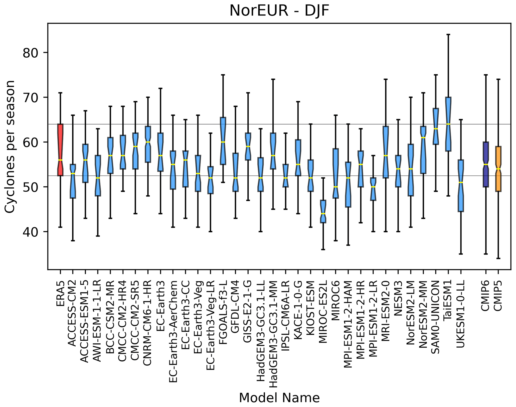
Figure A7Boxplots of cyclone numbers per DJF season for the NEU region (coordinates). Boxes are shown for ERA5 (red), 32 CMIP6 models (light blue), and the CMIP6 (purple) and CMIP5 model ensembles (orange). Boxes extend to the 25th and 75th percentiles of the distributions, with whiskers extending to 1.5 times the interquartile range. Horizonal yellow lines indicate the medians. Notches around the medians show its uncertainty based on 10 000 random resamples. Horizontal grey lines indicate the ERA5 25th and 75th percentiles.
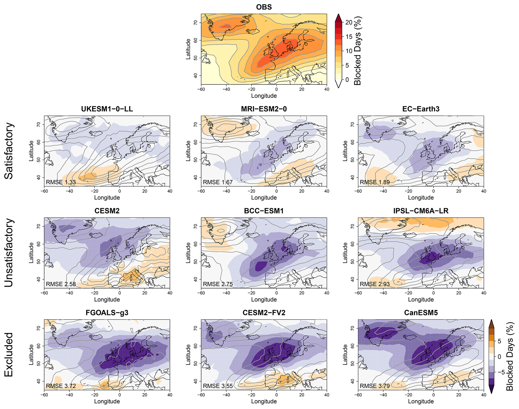
Figure A8Examples of DJF blocking-frequency classifications for a sample of individual models.
A4 Atlantic meridional overturning circulation
The representation of the AMOC is still considered to be deficient even in state-of-the-art GCMs, where its associated climate impacts are also thought to have been underestimated (Zhang et al., 2019). In addition, due to the limited availability of observational data, there is still considerable uncertainty in the recent AMOC evolution (Menary et al., 2020), and an accurate assessment of the AMOC in climate models remains challenging. For this study, some assessment of the AMOC is considered to be important due to its potential role in future changes in the European climate. The aim is to identify and flag the poorest models with large errors in the representation of the AMOC compared to the observational data from the rapid array (Frajka-Williams et al., 2021). Examples of the overturning stream function for each model shown (Fig. A6) are calculated using the method of Menary et al. (2020).
NESM3 and IPSL-CM6A-LR both show poor agreement with the observational data, with a consistently weak AMOC (Fig. A6). NESM3 was classified as inadequate, and the impact of the AMOC on the NA SSTs is also flagged due to a large cold bias. The AMOC for IPSL-CM6A-LR is flagged as unsatisfactory; the error may impact the representation of the NA, but the impact on the reliability of future projections is not clear. A similar error was present in CAMS-CSM1-0, which is also flagged as unsatisfactory. In contrast, the NorESM2-LM model has a consistently strong AMOC through the historical period, with a rapid decrease in more recent years, which is not seen in the observational data. This model is also classified as unsatisfactory. The other models for which AMOC data were available are classified as satisfactory (e.g.INM-CM4-8 and INM-CM5-0), as they do not show a large deviation from the observations.
A5 Storm tracks
A5.1 Regional assessment
The storm tracks were also assessed regionally to determine whether the number and variability of the cyclones in a particular region were captured satisfactorily by the models. This used the analysis of Priestley et al. (2020) for the individual European regions. The baseline time period used for this assessment is 1979/1980–2013 for CMIP6 (1979/1980–2004/2005 for CMIP5), and the model data are compared to ERA5.
Where the 25th and 75th percentiles of the range overlapped and were similar in size to the ERA5 data, the model was classified as satisfactory. If the interquartile range of the model had no overlap with ERA5 data or if the size of the interquartile range was substantially smaller, then the model was categorised as unsatisfactory for the region (see Fig. A7). Models are not excluded based on the regional analysis; these flags are for information only.
A6 Blocking frequency
Atmospheric blocking is a recurrent weather pattern typically occurring in the mid-latitudes at the exit of storm track (Rex, 1950; Pelly and Hoskins, 2003). It is characterised by a high-pressure low-potential-vorticity quasi-stationary large-scale anomaly which is able to block or divert the movement of the travelling cyclones, creating anomalous weather in its underlying region. One challenging issue for the climate community is the struggle that weather and climate models have in reproducing the observed frequency of atmospheric blocking (D'Andrea, 1998; Masato et al., 2013). Indeed, state-of-the-art climate models are known for underestimating the frequency of atmospheric blocking, especially over the Euro-Atlantic sector, albeit notable improvements have been observed with the last generation of models (Davini and d'Andrea, 2020).
In this work, atmospheric blocking is identified with an objective index based on the reversal of the daily geopotential height gradient measured at 500 hPa, making use of the blocking index developed by Davini et al. (2012). The index is the 2 d extension from 30 to 75∘ N of the canonical definition by Tibaldi and Molteni (1990). However, here, we adopt a blocking definition which includes a third supplementary condition south of the blocked region which is aimed at excluding the low-latitude blocking events (see Davini et al., 2012 for details). Defining Z500 as the daily geopotential height at 500 hPa interpolated on a common regular grid, the following three meridional gradients are considered:
where ϕ0 ranges from 30 to 75∘ N, while λ0 ranges from 0 to 360∘; ∘, ∘, and ∘. Instantaneous blocking is thus identified when
As done by Davini and d'Andrea (2020), no spatial or temporal filtering is applied.
A total of 29 CMIP6 models are taken into consideration for the time window 1961–2000. In order to define an objective method to classify into categories the atmospheric blocking bias over the Euro-Atlantic region (35–75∘ N, 60∘ W–40∘ E for winter and 45–75∘ N for summer, 60∘ W–40∘ E), two basic metrics has been introduced, namely the RMSE and Pearson correlation coefficient, evaluated against ERA5 reanalysis. Both RMSE and Pearson correlation coefficients are then standardised and used as non-dimensional parameters to perform a k-means clustering (Michelangeli et al., 1995), with k=3. In this way, climate models showing similar bias in both magnitude and pattern are clustered together, taking into account not only the size of the bias but also its shape. An example of the classification is provided in Fig. A8.
The code used to apply the ClimWIP method is publicly available via the ESMValTool (https://docs.esmvaltool.org/en/latest/recipes/recipe_climwip.html, ESMValTool, 2022). The data used in this study are available through the ESGF data portal at https://esgf-node.llnl.gov/projects/cmip6/ (CMIP, 2022). Further assessment plots for the models used in this paper are available on GitHub at https://github.com/tepmo42/cmip6_european_assessment (https://doi.org/10.5281/zenodo.782884, Palmer et al., 2023), as is a spreadsheet of all available assessments (for Europe) carried out for CMIP6 models to date. The RAPID-MOC monitoring project is funded by the Natural Environment Research Council and data (Frajka-Williams et al., 2021). E-OBS data (v.14.0, Cornes et al., 2018) can be found at https://www.ecad.eu/download/ensembles/download.php, in Cornes et al. (2018). The HadISST dataset (Rayner et al., 2003) is publicly available for download at https://www.metoffice.gov.uk/hadobs/hadisst/data/download.html. The ERA5 data (Hersbach et al., 2020) are available for download through the Copernicus Climate Change Service (2017) at https://cds.climate.copernicus.eu/cdsapp#!/home.
The supplement related to this article is available online at: https://doi.org/10.5194/esd-14-457-2023-supplement.
TEP: conceptualisation, data curation, formal analysis, investigation, methodology, software for data processing and analysis, supervision, validation, visualisation, writing – original draft, writing – review and editing. CFM: conceptualisation, funding acquisition, methodology, project administration, supervision, validation, writing – original draft, writing – review and editing. BBBB: conceptualisation, funding acquisition, methodology, project administration, supervision, validation, writing – original draft, writing – review and editing. MDKP: conceptualisation, data curation, formal analysis, software for data analysis (storm tracks), investigation, methodology, validation, visualisation, writing – original draft, writing – review and editing. PD: conceptualisation, data curation, formal analysis, software for data analysis (blocking frequency), investigation, methodology, validation, visualisation, writing – original draft, writing – review and editing. LuB: conceptualisation, methodology, validation, visualisation, software (ClimWIP method), writing – review and editing. LeB: conceptualisation, methodology, validation, writing – review and editing. MBM: validation, data curation, software for data processing and analysis for AMOC assessment, writing – review and editing.
The contact author has declared that none of the authors has any competing interests.
Publisher's note: Copernicus Publications remains neutral with regard to jurisdictional claims in published maps and institutional affiliations.
We acknowledge the World Climate Research Programme, which, through its Working Group on Coupled Modelling, coordinated and promoted CMIP5 and CMIP6. We thank the climate modelling groups (particularly those listed in Table S1 in the Supplement) for producing and making available their model output, the Earth System Grid Federation (ESGF) for archiving the data and providing access, and the multiple funding agencies who support CMIP, CMIP6 and ESGF. Terms of use and further instructions can be found at https://pcmdi.llnl.gov/ (last access: 14 April 2023). The work carried out for this paper was part of the EUCP project. We acknowledge the E-OBS dataset from the EU-FP6 project UERRA (http://www.uerra.eu, last access: 20 April 2023), the Copernicus Climate Change Service, and the data providers in the ECA&D project (https://www.ecad.eu, last access: 20 April 2023).
This research has been supported by Horizon 2020 (EUCP (grant no. 776613)). Leonard Borchert received funding from the Deutsche Forschungsgemeinschaft (DFG, German Research Foundation) under Germany's Excellence Strategy (EXC 2037, “Climate, Climatic Change and Society” – CLICCS, project no. 390683824) as a contribution to the Center for Earth System Research and Sustainability (CEN) of Universität Hamburg. Leonard Borchert was also funded by the ANR-Tremplin ERC project HARMONY (grant no. ANR-20-ERC9-0001). Matthew B. Menary was supported by the European Union Horizon 2020 project 4C, Climate–Carbon Interactions in the Coming Century (grant no. 821003) and the ANR-Tremplin ERC project HARMONY (grant no. ANR-20-ERC9-0001).
This paper was edited by Andrey Gritsun and reviewed by two anonymous referees.
Ashfaq, M., Rastogi, D., Kitson, J., Abid, M. A., and Kao, S.-C.: Evaluation of CMIP6 GCMs Over the CONUS for Downscaling Studies, J. Geophys. Res.-Atmos., 127, e2022JD036659, https://doi.org/10.1029/2022JD036659, 2022. a
Athanasiadis, P. J., Ogawa, F., Omrani, N.-E., Keenlyside, N., Schiemann, R., Baker, A. J., Vidale, P. L., Bellucci, A., Ruggieri, P., Haarsma, R., and Roberts, M.: Mitigating climate biases in the midlatitude North Atlantic by increasing model resolution: SST gradients and their relation to blocking and the jet, J. Clim., 35, 3385–3406, 2022. a
Bellomo, K., Angeloni, M., Corti, S., and von Hardenberg, J.: Future climate change shaped by inter-model differences in Atlantic meridional overturning circulation response, Nat. Commun., 12, 3659, https://doi.org/10.1038/s41467-021-24015-w, 2021. a
Bock, L., Lauer, A., Schlund, M., Barreiro, M., Bellouin, N., Jones, C., Meehl, G. A., Predoi, V., Roberts, M. J., and Eyring, V.: Quantifying Progress Across Different CMIP Phases With the ESMValTool, J. Geophys. Res.-Atmos., 125, e2019JD032321, https://doi.org/10.1029/2019JD032321, 2020. a, b
Booth, B. B. B., Dunstone, N. J., Halloran, P. R., Andrews, T., and Bellouin, N.: Aerosols implicated as a prime driver of twentieth-century North Atlantic climate variability, Nature, 484, 228–232, https://doi.org/10.1038/nature10946, 2012. a
Borchert, L. F., Pohlmann, H., Baehr, J., Neddermann, N.-C., Suarez-Gutierrez, L., and Müller, W. A.: Decadal Predictions of the Probability of Occurrence for Warm Summer Temperature Extremes, Geophys. Res. Lett., 46, 14042–14051, https://doi.org/10.1029/2019GL085385, 2019. a
Borchert, L. F., Koul, V., Menary, M. B., Befort, D. J., Swingedouw, D., Sgubin, G., and Mignot, J.: Skillful decadal prediction of unforced southern European summer temperature variations, Environ. Res. Lett., 16, 104017, https://doi.org/10.1088/1748-9326/ac20f5, 2021a. a
Borchert, L. F., Menary, M. B., Swingedouw, D., Sgubin, G., Hermanson, L., and Mignot, J.: Improved Decadal Predictions of North Atlantic Subpolar Gyre SST in CMIP6, Geophys. Res. Lett., 48, e2020GL091307, https://doi.org/10.1029/2020GL091307, 2021b. a, b, c
Börgel, F., Meier, H. E. M., Gröger, M., Rhein, M., Dutheil, C., and Kaiser, J. M.: Atlantic multidecadal variability and the implications for North European precipitation, Environ. Res. Lett., 17, 044040, https://doi.org/10.1088/1748-9326/ac5ca1, 2022. a
Browning, K. A.: The sting at the end of the tail: Damaging winds associated with extratropical cyclones, Q. J. Roy. Meteorol. Soc., 130, 375–399, https://doi.org/10.1256/qj.02.143, 2004. a
Brunner, L., Lorenz, R., Zumwald, M., and Knutti, R.: Quantifying uncertainty in European climate projections using combined performance-independence weighting, Environ. Res. Lett., 14, 124010, https://doi.org/10.1088/1748-9326/ab492f, 2019. a, b
Brunner, L., McSweeney, C., Ballinger, A. P., Befort, D. J., Benassi, M., Booth, B., Coppola, E., Vries, H. D., Harris, G., Hegerl, G. C., Knutti, R., Lenderink, G., Lowe, J., Nogherotto, R., O'Reilly, C., Qasmi, S., Ribes, A., Stocchi, P., and Undorf, S.: Comparing Methods to Constrain Future European Climate Projections Using a Consistent Framework, J. Clim., 33, 8671–8692, https://doi.org/10.1175/JCLI-D-19-0953.1, 2020a. a, b, c
Brunner, L., Pendergrass, A. G., Lehner, F., Merrifield, A. L., Lorenz, R., and Knutti, R.: Reduced global warming from CMIP6 projections when weighting models by performance and independence, Earth Syst. Dynam., 11, 995–1012, https://doi.org/10.5194/esd-11-995-2020, 2020b. a, b, c, d, e, f, g, h
Carvalho-Oliveira, J., Borchert, L. F., Duchez, A., Dobrynin, M., and Baehr, J.: Subtle influence of the Atlantic Meridional Overturning Circulation (AMOC) on seasonal sea surface temperature (SST) hindcast skill in the North Atlantic, Weather Clim. Dynam., 2, 739–757, https://doi.org/10.5194/wcd-2-739-2021, 2021. a
Carvalho-Oliveira, J., Borchert, L. F., Zorita, E., and Baehr, J.: Self-Organizing Maps Identify Windows of Opportunity for Seasonal European Summer Predictions, Front. Clim., 4, 844634, https://doi.org/10.3389/fclim.2022.844634, 2022. a
Chaudhuri, A. H., Ponte, R. M., and Nguyen, A. T.: A Comparison of Atmospheric Reanalysis Products for the Arctic Ocean and Implications for Uncertainties in Air–Sea Fluxes, J. Clim., 27, 5411–5421, https://doi.org/10.1175/JCLI-D-13-00424.1, 2014. a
Chen, Z., Zhou, T., Chen, X., Zhang, W., Zhang, L., Wu, M., and Zou, L.: Observationally constrained projection of Afro-Asian monsoon precipitation, Nat. Commun., 13, 2552, https://doi.org/10.1038/s41467-022-30106-z, 2022. a
CMIP: Coupled Model Intercomparison Project Phase 6 (CMIP6) data, Working Group on Coupled Modeling of the World Climate Research Programme, Earth System Grid Federation [data set], https://esgf-node.llnl.gov/projects/cmip6/, last access: 3 August 2022. a
Copernicus Climate Change Service (C3S): ERA5: Fifth generation of ECMWF atmospheric reanalyses of the global climate, Copernicus Climate Change Service Climate Data Store (CDS) [data set], https://cds.climate.copernicus.eu/cdsapp#!/home (last access: October 2020), 2017. a
Cornes, R., van der Schrier, G., van den Besselaar, E. J. M., and Jones, P. D.: An Ensemble Version of the E-OBS Temperature and Precipitation Datasets, J. Geophys. Res.-Atmos., 123, https://doi.org/10.1029/2017JD028200, 2018 (data available at https://www.ecad.eu/download/ensembles/download.php, last access: 19 April 2023). a, b, c, d
D'Andrea, F.: Northern Hemisphere atmospheric blocking as simulated by 15 atmospheric general circulation models in the period 1979–1988, Clim. Dynam., 14, 385–407, https://doi.org/10.1007/s003820050230, 1998. a
Davini, P. and d'Andrea, F.: From CMIP3 to CMIP6: Northern hemisphere atmospheric blocking simulation in present and future climate, J. Clim., 33, 10021–10038, https://doi.org/10.1175/JCLI-D-19-0862.1, 2020. a, b, c, d, e
Davini, P., Cagnazzo, C., Gualdi, S., and Navarra, A.: Bidimensional diagnostics, variability and trends of Northern Hemisphere blocking, J. Clim., 25, 6496–6509, https://doi.org/10.1175/JCLI-D-12-00032.1, 2012. a, b
Dong, B., Sutton, R. T., Woollings, T., and Hodges, K.: Variability of the North Atlantic summer storm track: mechanisms and impacts on European climate, Environ. Res. Lett., 8, 034037, https://doi.org/10.1088/1748-9326/8/3/034037, 2013. a
ESMValTool: Earth System Model Evaluation Tool, Zenodo [code], https://doi.org/10.5281/zenodo.3401363 and https://doi.org/10.5281/zenodo.3387139, 2022. a
Eyring, V., Bony, S., Meehl, G. A., Senior, C. A., Stevens, B., Stouffer, R. J., and Taylor, K. E.: Overview of the Coupled Model Intercomparison Project Phase 6 (CMIP6) experimental design and organization, Geosci. Model Dev., 9, 1937–1958, https://doi.org/10.5194/gmd-9-1937-2016, 2016. a
Eyring, V., Cox, P. M., Flato, G. M., Gleckler, P. J., Abramowitz, G., Caldwell, P., Collins, W. D., Gier, B. K., Hall, A. D., Hoffman, F. M., Hurtt, G. C., Jahn, A., Jones, C. D., Klein, S. A., Krasting, J. P., Kwiatkowski, L., Lorenz, R., Maloney, E., Meehl, G. A., Pendergrass, A. G., Pincus, R., Ruane, A. C., Russell, J. L., Sanderson, B. M., Santer, B. D., Sherwood, S. C., Simpson, I. R., Stouffer, R. J., and Williamson, M. S.: Taking climate model evaluation to the next level, Nat. Clim. Change, 9, 102–110, https://doi.org/10.1038/s41558-018-0355-y, 2019. a
Flato, G., Marotzke, J., Abiodun, B., Braconnot, P., Chou, S. C., Collins, W., Cox, P., Driouech, F., Emori, S., Eyring, V., Forest, C., Gleckler, P., Guilyardi, E., Jakob, C., Kattsov, V., Reason, C., and Rummukainen, M.: Evaluation of climate models, Cambridge University Press, Cambridge, UK, 741–882, https://doi.org/10.1017/CBO9781107415324.020, 2013. a
Forster, P., Storelvmo, T., Armour, K., Collins, W., Dufresne, J.-L., Frame, D., Lunt, D. J., Mauritsen, T., Palmer, M. D., Watanabe, M., Wild, M., and Zhang, H.: The Earth's Energy Budget, Climate Feedbacks, and Climate Sensitivity, in: Climate Change 2021: The Physical Science Basis. Contribution of Working Group I to the Sixth Assessment Report of the Intergovernmental Panel on Climate Change, edited by: Masson-Delmotte, V., Zhai, P., Pirani, A., Connors, S. L., Péan, C., Berger, S., Caud, N., Chen, Y., Goldfarb, L., Gomis, M. I., Huang, M., Leitzell, K., Lonnoy, E., Matthews,J. B. R., Maycock, T. K., Waterfield, T., Yelekçi, O., Yu, R., and Zhou, B., Cambridge University Press, Cambridge, United Kingdom and New York, NY, USA, 923–1054, 2021. a
Frajka-Williams, E., Moat, B. I., Smeed, D. A., Rayner, D., Johns, W. E., Baringer, M. O., Volkov, D., and Collins, J.: Atlantic meridional overturning circulation observed by the RAPID-MOCHA-WBTS (RAPID-Meridional Overturning Circulation and Heatflux Array-Western Boundary Time Series) array at 26N from 2004 to 2020 (v2020.1), British Oceanographic Data Centre – Natural Environment Research Council, UK [data set], https://doi.org/10.5285/cc1e34b3-3385-662b-e053-6c86abc03444, 2021. a, b
Gervais, M., Shaman, J., and Kushnir, Y.: Impacts of the North Atlantic Warming Hole in Future Climate Projections: Mean Atmospheric Circulation and the North Atlantic Jet, J. Clim., 32, 2673–2689, https://doi.org/10.1175/JCLI-D-18-0647.1, 2019. a
Gutiérrez, J., Jones, R., Narisma, G., Alves, L., Amjad, M., Gorodetskaya, I., Grose, M., Klutse, N., S.Krakovska, Li, J., Martínez-Castro, D., Mearns, L., Mernild, S., Ngo-Duc, T., van den Hurk, B., and Yoon, J.-H.: Atlas, in: Climate Change 2021: The Physical Science Basis, Contribution of Working Group I to the Sixth Assessment Report of the Intergovernmental Panel on Climate Change, edited by: Masson-Delmotte, V., Zhai, P., Pirani, A., Connors, S., Péan, C., Berger, S., Caud, N., Chen, Y., Goldfarb, L., Gomis, M., Huang, M., Leitzell, K., Lonnoy, E., Matthews, J., Maycock, T., Waterfield, T., Yelekçi, O., Yu, R., and Zhou, B., chap. Atlas, Cambridge University Press, Cambridge, United Kingdom and New York, NY, USA, 1927–2058, 2021. a, b, c
Hausfather, Z., Marvel, K., Schmidt, G. A., Nielsen-Gammon, J. W., and Zelinka, M.: Climate simulations: recognize the “hot model” problem, Nature, 605, 26–29, https://doi.org/10.1038/d41586-022-01192-2, 2022. a, b
Hempel, S., Frieler, K., Warszawski, L., Schewe, J., and Piontek, F.: A trend-preserving bias correction – the ISI-MIP approach, Earth Syst. Dynam., 4, 219–236, https://doi.org/10.5194/esd-4-219-2013, 2013. a
Hersbach, H., Bell, B., Berrisford, P., et al.: The ERA5 global reanalysis, Q. J. R. Meteorol. Soc., 146, 1999–2049, https://doi.org/10.1002/qj.3803, 2020. a, b
Hodges, K.: Feature tracking on the unit sphere, Mon. Weather Rev., 123, 3458–3465, 1995. a
Hodges, K. I.: A General Method for Tracking Analysis and Its Application to Meteorological Data, Mon. Weather Rev., 122, 2573–2586, https://doi.org/10.1175/1520-0493(1994)122<2573:AGMFTA>2.0.CO;2, 1994. a
IPCC, 2007: Climate Change 2007: The Physical Science Basis. Contribution of Working Group I to the Fourth Assessment Report of the Intergovernmental Panel on Climate Change, edited by: Solomon, S., Qin, D., Manning, M., Chen, Z., Marquis, M., Averyt, K. B., Tignor, M., and Miller, H. L., Cambridge University Press, Cambridge, United Kingdom and New York, NY, USA, 996 pp., https://www.ipcc.ch/report/ar4/wg1/ (last access: 14 April 2023), 2007. a
IPCC: Climate Change 2013: The Physical Science Basis. Contribution of Working Group I to the Fifth Assessment Report of the Intergovernmental Panel on Climate Change, edited by: Stocker, T. F., Qin, D., Plattner, G.-K., Tignor, M., Allen, S. K., Boschung, J., Nauels, A., Xia, Y., Bex, V., and Midgley, P. M., Cambridge University Press, Cambridge, United Kingdom and New York, NY, USA, 1535 pp., https://www.ipcc.ch/report/ar5/wg1/ (last access: 14 April 2023), 2013. a
Ito, R., Shiogama, H., Nakaegawa, T., and Takayabu, I.: Uncertainties in climate change projections covered by the ISIMIP and CORDEX model subsets from CMIP5, Geosci. Model Dev., 13, 859–872, https://doi.org/10.5194/gmd-13-859-2020, 2020. a
Jackson, L. C., Biastoch, A., Buckley, M. W., Desbruyères, D. G., Frajka-Williams, E., Moat, B., and Robson, J.: The evolution of the North Atlantic Meridional Overturning Circulation since 1980, Nat. Rev. Earth Environ., 3, 241–254, https://doi.org/10.1038/s43017-022-00263-2, 2022. a
Jin, C., Wang, B., and Liu, J.: Future Changes and Controlling Factors of the Eight Regional Monsoons Projected by CMIP6 Models, J. Clim., 33, 9307–9326, https://doi.org/10.1175/JCLI-D-20-0236.1, 2020. a
Kaspi, Y. and Schneider, T.: The Role of Stationary Eddies in Shaping Midlatitude Storm Tracks, J. Atmos. Sci., 70, 2596–2613, https://doi.org/10.1175/JAS-D-12-082.1, 2013. a
Keeley, S. P. E., Sutton, R. T., and Shaffrey, L. C.: The impact of North Atlantic sea surface temperature errors on the simulation of North Atlantic European region climate, Q. J. Roy. Meteorol. Soc., 138, 1774–1783, https://doi.org/10.1002/qj.1912, 2012. a, b, c
Knutti, R.: The end of model democracy?, Climatic Change, 102, 395–404, https://doi.org/10.1007/s10584-010-9800-2, 2010. a, b
Knutti, R., Sedláček, J., Sanderson, B. M., Lorenz, R., Fischer, E. M., and Eyring, V.: A climate model projection weighting scheme accounting for performance and interdependence, Geophys. Res. Lett., 44, 1909–1918, https://doi.org/10.1002/2016GL072012, 2017. a, b
Lange, S. and Büchner, M.: ISIMIP3b bias-adjusted atmospheric climate input data (v1.1), ISIMIP Repository, https://doi.org/10.48364/ISIMIP.842396.1, 2021. a
Lee, R. W., Woollings, T. J., Hoskins, B. J., Williams, K. D., O'Reilly, C. H., and Masato, G.: Impact of Gulf Stream SST biases on the global atmospheric circulation, Clim. Dynam., 51, 3369–3387, https://doi.org/10.1007/s00382-018-4083-9, 2018. a
Liang, Y., Gillett, N. P., and Monahan, A. H.: Climate Model Projections of 21st Century Global Warming Constrained Using the Observed Warming Trend, Geophys. Res. Lett., 47, e2019GL086757, https://doi.org/10.1029/2019GL086757, 2020. a, b, c, d, e
Lorenz, R., Herger, N., Sedláček, J., Eyring, V., Fischer, E. M., and Knutti, R.: Prospects and Caveats of Weighting Climate Models for Summer Maximum Temperature Projections Over North America, J. Geophys. Res.-Atmos., 123, 4509–4526, https://doi.org/10.1029/2017JD027992, 2018. a
Lutz, A. F., ter Maat, H. W., Biemans, H., Shrestha, A. B., Wester, P., and Immerzeel, W. W.: Selecting representative climate models for climate change impact studies: an advanced envelope-based selection approach, Int. J. Clim., 36, 3988–4005, https://doi.org/10.1002/joc.4608, 2016. a, b
Mahony, C. R., Wang, T., Hamann, A., and Cannon, A. J.: A global climate model ensemble for downscaled monthly climate normals over North America, Int. J. Climatol., 42, 5871–5891, https://doi.org/10.1002/joc.7566, 2022. a
Masato, G., Hoskins, B. J., and Woollings, T.: Winter and summer Northern Hemisphere blocking in CMIP5 models, J. Clim., 26, 7044–7059, https://doi.org/10.1175/JCLI-D-12-00466.1, 2013. a
McDermid, S. P., Ruane, A. C., Rosenzweig, C., Hudson, N. I., Morales, M. D., Agalawatte, P., Ahmad, S., Ahuja, L. R., Amien, I., Anapalli, S. S., Anothai, J., Asseng, S., Biggs, J., Bert, F., Bertuzzi, P., Bhatia, V. S., Bindi, M., Broad, I., Cammarano, D., Carretero, R., Chattha, A. A., Chung, U., Debats, S., Deligios, P., De Sanctis, G., Dhliwayo, T., Dumont, B., Estes, L., Ewert, F., Ferrise, R., Gaiser, T., Garcia, G., Gbegbelegbe, S., Geethalakshmi, V., Gerardeaux, E., Goldberg, R., Grant, B., Guevara, E., Hickman, J., Hoffmann, H., Huang, H., Hussain, J., Justino, F. B., Karunaratne, A. S., Koehler, A.-K., Kouakou, P. K., Kumar, S. N., Lakshmanan, A., Lieffering, M., Lin, X., Luo, Q., Magrin, G., Mancini, M., Marin, F. R., Marta, A. D., Masutomi, Y., Mavromatis, T., McLean, G., Meira, S., Mohanty, M., Moriondo, M., Nasim, W., Negm, L., Orlando, F., Orlandini, S., Ozturk, I., Soares Pinto, H. M., Podesta, G., Qi, Z., Ramarohetra, J., ur Rahman, M. H., Raynal, H., Rodriguez, G., Rötter, R., Sharda, V., Shuo, L., Smith, W., Snow, V., Soltani, A., Srinivas, K., Sultan, B., Swain, D. K., Tao, F., Tesfaye, K., Travasso, M. I., Trombi, G., Topaj, A., Vanuytrecht, E., Viscarra, F. E., Aftab Wajid, S., Wang, E., Wang, H., Wang, J., Wijekoon, E., Byun-Woo, L., Xiaoguang, Y., Young, B. H., Yun, J. I., Zhao, Z., and Zubair, L.: The AgMIP Coordinated Climate-Crop Modeling Project (C3MP): Methods and Protocols, in: Handbook of Climate Change and Agroecosystems, Vol. 3, ICP Series on Climate Change Impacts, Adaptation, and Mitigation, 191–220, IMPERIAL COLLEGE PRESS, https://doi.org/10.1142/9781783265640_0008, 2014. a
McSweeney, C., Murphy, J., Sexton, D., Rostron, J., Yamazaki, K., and Harris, G.: Selection of CMIP5 members to augment a perturbed–parameter ensemble of global realisations of future climate for the UKCP18 scenarios, Tech. rep., Hadley Centre Technical Note 102, HCTN_102_2018P, Met Office UA, 2018. a, b, c
McSweeney, C. F. and Jones, R. G.: How representative is the spread of climate projections from the 5 CMIP5 GCMs used in ISI-MIP?, Clim. Serv., 1, 24–29, https://doi.org/10.1016/j.cliser.2016.02.001, 2016. a
McSweeney, C. F., Jones, R. G., and Booth, B. B. B.: Selecting Ensemble Members to Provide Regional Climate Change Information, J. Clim., 25, 7100–7121, https://doi.org/10.1175/JCLI-D-11-00526.1, 2012. a
McSweeney, C. F., Jones, R. G., Lee, R. W., and Rowell, D. P.: Selecting CMIP5 GCMs for downscaling over multiple regions, Clim. Dynam., 44, 3237–3260, https://doi.org/10.1007/s00382-014-2418-8, 2015. a, b, c, d, e, f, g, h
Menary, M. B., Robson, J., Allan, R. P., Booth, B. B. B., Cassou, C., Gastineau, G., Gregory, J., Hodson, D., Jones, C., Mignot, J., Ringer, M., Sutton, R., Wilcox, L., and Zhang, R.: Aerosol‐Forced AMOC Changes in CMIP6 Historical Simulations, Geophys. Res. Lett., 47, e2020GL088166, https://doi.org/10.1029/2020GL088166, 2020. a, b, c, d, e
Merrifield, A. L., Brunner, L., Lorenz, R., Medhaug, I., and Knutti, R.: An investigation of weighting schemes suitable for incorporating large ensembles into multi-model ensembles, Earth Syst. Dynam., 11, 807–834, https://doi.org/10.5194/esd-11-807-2020, 2020. a, b
Michelangeli, P.-A., Vautard, R., and Legras, B.: Weather Regimes: Recurrence and Quasi Stationarity, J. Atmos. Sci., 52, 1237–1256, https://doi.org/10.1175/1520-0469(1995)052<1237:WRRAQS>2.0.CO;2, 1995. a
Bukovsky, M. S., Thompson, J. A., and Mearns, L. O.: Weighting a regional climate model ensemble: Does it make a difference? Can it make a difference?, Clim. Res., 77, 23–43, 2019. a, b
Ossó, A., Sutton, R., Shaffrey, L., and Dong, B.: Development, Amplification, and Decay of Atlantic/European Summer Weather Patterns Linked to Spring North Atlantic Sea Surface Temperatures, J. Clim., 33, 5939–5951, https://doi.org/10.1175/JCLI-D-19-0613.1, 2020. a, b
Oudar, T., Cattiaux, J., and Douville, H.: Drivers of the Northern Extratropical Eddy-Driven Jet Change in CMIP5 and CMIP6 Models, Geophys. Res. Lett., 47, e2019GL086695, https://doi.org/10.1029/2019GL086695, 2020. a
Overland, J. E., Wang, M., Bond, N. A., Walsh, J. E., Kattsov, V. M., and Chapman, W. L.: Considerations in the Selection of Global Climate Models for Regional Climate Projections: The Arctic as a Case Study, J. Clim., 24, 1583–1597, https://doi.org/10.1175/2010JCLI3462.1, 2011. a, b
Palmer, T. E., Booth, B. B. B., and McSweeney, C. F.: How does the CMIP6 ensemble change the picture for European climate projections?, Environ. Res. Lett., 16, 094042, https://doi.org/10.1088/1748-9326/ac1ed9, 2021. a
Palmer, T. E., McSweeney, C. F., Booth, B. B. B., Priestley, M. D. K., Davini, P., Brunner, L., Borchert, L., and Menary, M. B.: tepmo42/cmip6_european_assessment: Performance-based sub-selection of CMIP6 models for impact assessments in Europe additional plots, Zenodo [data set], https://doi.org/10.5281/zenodo.7828845, 2023. a
Pelly, J. and Hoskins, B.: A new perspective on blocking, J. Atmos. Sci., 60, 743–755, https://doi.org/10.1175/1520-0469(2003)060<0743:ANPOB>2.0.CO;2, 2003. a
Prein, A. F., Bukovsky, M. S., Mearns, L. O., Bruyère, C. L., and Done, J. M.: Simulating North American Weather Types With Regional Climate Models, Front. Environ. Sci., 7, p. 36, 2019. a, b
Priestley, M. D., Ackerley, D., Catto, J. L., Hodges, K. I., McDonald, R. E., and Lee, R. W.: An Overview of the Extratropical Storm Tracks in CMIP6 Historical Simulations, J. Clim., 33, 6315–6343, https://doi.org/10.1175/JCLI-D-19-0928.1, 2020. a, b, c, d, e, f
Priestley, M. D. K., Ackerley, D., Catto, J. L., and Hodges, K. I.: Drivers of Biases in the CMIP6 Extratropical Storm Tracks, Part I: Northern Hemisphere, J. Clim., 36, 1451–1467, https://doi.org/10.1175/JCLI-D-20-0976.1, 2023. a, b, c
Rayner, N. A., Parker, D. E., Horton, E. B., Folland, C. K., Alexander, L. V., Rowell, D. P., Kent, E. C., and Kaplan, A.: Global analyses of sea surface temperature, sea ice, and night marine air temperature since the late nineteenth century, J. Geophys. Res., 108, 4407, https://doi.org/10.1029/2002JD002670, 2003 (data available at https://www.metoffice.gov.uk/hadobs/hadisst/data/download.html, last access: December 2022). a, b
Rex, D.: Blocking action in the middle troposphere and its effect upon regional climate: I. An aerological study of blocking action, Tellus, 2, 196–211, 1950. a
Ribes, A., Qasmi, S., and Gillett, N. P.: Making climate projections conditional on historical observations, Sci. Adv., 7, eabc0671, https://doi.org/10.1126/sciadv.abc0671, 2021. a, b, c, d, e
Ribes, A., Boé, J., Qasmi, S., Dubuisson, B., Douville, H., and Terray, L.: An updated assessment of past and future warming over France based on a regional observational constraint, Earth Syst. Dynam., 13, 1397–1415, https://doi.org/10.5194/esd-13-1397-2022, 2022. a, b, c
Rosenzweig, C., Arnell, N. W., Ebi, K. L., Lotze-Campen, H., Raes, F., Rapley, C., Smith, M. S., Cramer, W., Frieler, K., Reyer, C. P., Schewe, J., Van Vuuren, D., and Warszawski, L.: Assessing inter-sectoral climate change risks: The role of ISIMIP, Environ. Res. Lett., 12, 010301, https://doi.org/10.1088/1748-9326/12/1/010301, 2017. a
Ruane, A. C. and McDermid, S. P.: Selection of a representative subset of global climate models that captures the profile of regional changes for integrated climate impacts assessment, Earth Perspect., 4, 1–20, https://doi.org/10.1186/s40322-017-0036-4, 2017. a, b, c
Ruane, A. C., McDermid, S., Rosenzweig, C., Baigorria, G. A., Jones, J. W., Romero, C. C., and DeWayne Cecil, L.: Carbon–Temperature–Water change analysis for peanut production under climate change: a prototype for the AgMIP Coordinated Climate-Crop Modeling Project (C3MP), Glob. Change Biol., 20, 394–407, https://doi.org/10.1111/gcb.12412, 2014. a
Scaife, A. A., Copsey, D., Gordon, C., Harris, C., Hinton, T., Keeley, S., O'Neill, A., Roberts, M., and Williams, K.: Improved Atlantic winter blocking in a climate model, Geophys. Res. Lett., 38, L23703, https://doi.org/10.1029/2011GL049573, 2011. a, b
Schiemann, R., Athanasiadis, P., Barriopedro, D., Doblas-Reyes, F., Lohmann, K., Roberts, M. J., Sein, D. V., Roberts, C. D., Terray, L., and Vidale, P. L.: Northern Hemisphere blocking simulation in current climate models: evaluating progress from the Climate Model Intercomparison Project Phase 5 to 6 and sensitivity to resolution, Weather Clim. Dynam., 1, 277–292, https://doi.org/10.5194/wcd-1-277-2020, 2020. a
Selten, F. M., Bintanja, R., Vautard, R., and van den Hurk, B. J. J. M.: Future continental summer warming constrained by the present-day seasonal cycle of surface hydrology, Sci. Rep., 10, 4721, https://doi.org/10.1038/s41598-020-61721-9, 2020. a
Shepherd, T. G.: Atmospheric circulation as a source of uncertainty in climate change projections, Nat. Geosci., 7, 703–708, https://doi.org/10.1038/ngeo2253, 2014. a
Shepherd, T. G.: Storyline approach to the construction of regional climate change information, Proc. Roy. Soc. A, 475, 20190013, https://doi.org/10.1098/rspa.2019.0013, 2019. a
Shiogama, H., Ishizaki, N. N., Hanasaki, N., Takahashi, K., Emori, S., Ito, R., Nakaegawa, T., Takayabu, I., Hijioka, Y., Takayabu, Y. N., and Shibuya, R.: Selecting CMIP6-Based Future Climate Scenarios for Impact and Adaptation Studies, SOLA, 17, 57–62, https://doi.org/10.2151/sola.2021-009, 2021. a, b
Simpson, I. R., Deser, C., McKinnon, K. A., and Barnes, E. A.: Modeled and Observed Multidecadal Variability in the North Atlantic Jet Stream and Its Connection to Sea Surface Temperatures, J. Clim., 31, 8313–8338, https://doi.org/10.1175/JCLI-D-18-0168.1, 2018. a
Sutton, R. T. and Dong, B.: Atlantic Ocean influence on a shift in European climate in the 1990s, Nat. Geosci., 5, 788–792, https://doi.org/10.1038/ngeo1595, 2012. a, b
Tibaldi, S. and Molteni, F.: On the operational predictability of blocking, Tellus A, 42, 343–365, https://doi.org/10.3402/tellusa.v42i3.11882, 1990. a
Tokarska, K. B., Stolpe, M. B., Sippel, S., Fischer, E. M., Smith, C. J., Lehner, F., and Knutti, R.: Past warming trend constrains future warming in CMIP6 models, Sci. Adv., 6, eaaz9549, https://doi.org/10.1126/sciadv.aaz9549, 2020. a, b, c, d, e
Tsujino, H., Urakawa, L. S., Griffies, S. M., Danabasoglu, G., Adcroft, A. J., Amaral, A. E., Arsouze, T., Bentsen, M., Bernardello, R., Böning, C. W., Bozec, A., Chassignet, E. P., Danilov, S., Dussin, R., Exarchou, E., Fogli, P. G., Fox-Kemper, B., Guo, C., Ilicak, M., Iovino, D., Kim, W. M., Koldunov, N., Lapin, V., Li, Y., Lin, P., Lindsay, K., Liu, H., Long, M. C., Komuro, Y., Marsland, S. J., Masina, S., Nummelin, A., Rieck, J. K., Ruprich-Robert, Y., Scheinert, M., Sicardi, V., Sidorenko, D., Suzuki, T., Tatebe, H., Wang, Q., Yeager, S. G., and Yu, Z.: Evaluation of global ocean–sea-ice model simulations based on the experimental protocols of the Ocean Model Intercomparison Project phase 2 (OMIP-2), Geosci. Model Dev., 13, 3643–3708, https://doi.org/10.5194/gmd-13-3643-2020, 2020. a
van den Hurk, B., Siegmund, P., Klien Tank (Eds), A., Attema, J., Bakker, A., Beersma, J., Bessembinder, J., Boers, R., Brandsma, T., van de Brink, H., Drijfhout, S., Eskes, H., Haarsma, R., Hazeleger, W., Jilderda, R., Katsman, C., Lenderink, G., Loriaux, J., van de Meijgaard, E., van Noije, T., van Oldenborgh, G. J., Selten, F., Siebesma, P., Sterl, A., de Vries, H., Van Weele, M., de Winter, R., and van Zadelhoff, G.-J.: KNMI'14: Climate Change scenarios for the 21st Century – A Netherlands perspective, Tech. Rep., Royal Netherlands Meteorological Istitute Ministry of Infrastructure and Water Management, https://www.knmiprojects.nl/projects/climate-scenarios (last access: 14 April 2023), 2014. a
Whetton, P., Macadam, I., Bathols, J., and O'Grady, J.: Assessment of the use of current climate patterns to evaluate regional enhanced greenhouse response patterns of climate models, Geophys. Res. Lett., 34, L14701, https://doi.org/10.1029/2007GL030025, 2007. a, b, c
White, J. W., Hoogenboom, G., Kimball, B. A., and Wall, G. W.: Methodologies for simulating impacts of climate change on crop production, Field Crop. Res., 124, 357–368, https://doi.org/10.1016/j.fcr.2011.07.001, 2011. a
Yeager, S. G. and Robson, J. I.: Recent Progress in Understanding and Predicting Atlantic Decadal Climate Variability, Curr. Clim. Change Rep., 3, 112–127, https://doi.org/10.1007/s40641-017-0064-z, 2017. a
Zappa, G. and Shepherd, T. G.: Storylines of atmospheric circulation change for European regional climate impact assessment, J. Clim., 30, 6561–6577, https://doi.org/10.1175/JCLI-D-16-0807.1, 2017. a
Zappa, G., Shaffrey, L. C., and Hodges, K. I.: The ability of CMIP5 models to simulate North Atlantic extratropical cyclones, J. Clim., 26, 5379–5396, https://doi.org/10.1175/JCLI-D-12-00501.1, 2013. a
Zhang, M.-Z., Xu, Z., Han, Y., and Guo, W.: Evaluation of CMIP6 models toward dynamical downscaling over 14 CORDEX domains, Clim. Dynam., 1–15, https://doi.org/10.1007/s00382-022-06355-5, 2022. a, b
Zhang, R.: Coherent surface-subsurface fingerprint of the Atlantic meridional overturning circulation, Geophys. Res. Lett., 35, L20705, https://doi.org/10.1029/2008GL035463, 2008. a
Zhang, R., Sutton, R., Danabasoglu, G., Kwon, Y., Marsh, R., Yeager, S. G., Amrhein, D. E., and Little, C. M.: A Review of the Role of the Atlantic Meridional Overturning Circulation in Atlantic Multidecadal Variability and Associated Climate Impacts, Rev. Geophys., 57, 316–375, https://doi.org/10.1029/2019RG000644, 2019. a, b
- Abstract
- Copyright statement
- Applications and motivations for regional sub-selection
- Performance assessment for Europe
- Materials and methods
- Results: assessment and applications for sub-selection
- Discussion
- Conclusions
- Appendix A
- Code and data availability
- Author contributions
- Competing interests
- Disclaimer
- Acknowledgements
- Financial support
- Review statement
- References
- Supplement