the Creative Commons Attribution 4.0 License.
the Creative Commons Attribution 4.0 License.
 | 01 Mar 2023
Ensemble forecast of an index of the Madden–Julian Oscillation using a stochastic weather generator based on circulation analogs
Riccardo Silini
Pascal Yiou
The Madden–Julian Oscillation (MJO) is one of the main sources of sub-seasonal atmospheric predictability in the tropical region. The MJO affects precipitation over highly populated areas, especially around southern India. Therefore, predicting its phase and intensity is important as it has a high societal impact. Indices of the MJO can be derived from the first principal components of zonal wind and outgoing longwave radiation (OLR) in the tropics (RMM1 and RMM2 indices). The amplitude and phase of the MJO are derived from those indices. Our goal is to forecast these two indices on a sub-seasonal timescale. This study aims to provide an ensemble forecast of MJO indices from analogs of the atmospheric circulation, computed from the geopotential at 500 hPa (Z500) by using a stochastic weather generator (SWG). We generate an ensemble of 100 members for the MJO amplitude for sub-seasonal lead times (from 2 to 4 weeks). Then we evaluate the skill of the ensemble forecast and the ensemble mean using probabilistic scores and deterministic skill scores. According to score-based criteria, we find that a reasonable forecast of the MJO index could be achieved within 40 d lead times for the different seasons. We compare our SWG forecast with other forecasts of the MJO. The comparison shows that the SWG forecast has skill compared to ECMWF forecasts for lead times above 20 d and better skill compared to machine learning forecasts for small lead times.
- Article
(7469 KB) - Full-text XML
- BibTeX
- EndNote


Forecasting the Madden–Julian Oscillation (MJO) is a crucial scientific endeavor as the MJO represents one of the most important sources of sub-seasonal predictability in the tropics. The Madden–Julian Oscillation controls tropical convection, with a life cycle going from 30 to 60 d (Lin et al., 2008). It is characterized by a dominant eastward propagation over the tropical Indo-Pacific basin, in particular during the boreal winter. The MJO affects the Indian and Australian monsoons (Zhang, 2013) and West African monsoon (Barlow et al., 2016). It was shown that it affects precipitation in East Asia (Zhang et al., 2013) and North America (Becker et al., 2011). The MJO affects the global weather as it impacts the tropics as well as the extratropics due to the atmospheric teleconnections (Zhang, 2013; Cassou, 2008).
The improvement of the forecast skill of the MJO is the subject of several studies. Numerical models have shown an ability to forecast the MJO index (Kim et al., 2018). However, the forecast of the MJO is sensitive to the quality of the initial conditions (Zhang, 2013; Straub, 2013). This motivates probabilistic forecasts to overcome the chaotic nature of climate variability (Sivillo et al., 1997; Palmer, 2000). Indeed, ensemble forecasts have shown improvements over deterministic forecasts for weather and climatic variables in the short and long term (Yiou and Déandréis, 2019; Hersbach et al., 2020). One of the advantages of ensemble forecasts is that they provide information about the forecast uncertainties, which deterministic forecasts cannot provide. In addition, the use of ensemble means has shown better forecast results than the individual ensemble members in previous works (Toth and Kalnay, 1997; Grimit and Mass, 2002; Xiang et al., 2015).
Statistical models, such as stochastic weather generators (SWGs), have been used for this purpose. SWGs are designed to mimic the behavior of climate variables (Ailliot et al., 2015). They have been used to forecast various weather and climatic variables such as temperature (Yiou and Déandréis, 2019), precipitation (Krouma et al., 2021), and the North Atlantic Oscillation (NAO) (Yiou and Déandréis, 2019). One of the benefits of using stochastic weather generators is that they have a low computing cost compared to numerical models. Combining stochastic weather generators with analogs of the atmospheric circulation is an efficient approach to generate ensemble weather forecasts with consistent atmospheric patterns (Yiou and Déandréis, 2019; Krouma et al., 2021; Blanchet et al., 2018).
Analogs of circulation were designed to provide forecasts assuming that similar situations in the atmospheric circulation could lead to similar local weather conditions (Lorenz, 1969). Recent studies have evaluated the potential of analogs to forecast the probability distribution of climate variables: Yiou and Déandréis (2019) simulated ensemble members of temperature using random sampling of atmospheric circulation analogs; Atencia and Zawadzki (2014) used analogs of precipitation to forecast precipitation.
The goal of this study is to forecast a daily MJO index for a sub-seasonal lead time (≈2–4 weeks) with a SWG based on analogs of the atmospheric circulation, described in Sect. 3.2. The SWG approach was evaluated in previous studies by Yiou and Déandréis (2019) and Krouma et al. (2021) for European temperature and precipitation. The SWG was able to forecast the temperature within 40 d and the precipitation within 20 d with reasonable skill scores in western Europe (Krouma et al., 2021; Yiou and Déandréis, 2019). In this paper, we adjust the parameters of the SWG in order to forecast the MJO indices. More precisely, our goals are (i) to forecast the MJO amplitude (directly from the amplitude and using the MJO indices) and (ii) to evaluate the ability of our SWG model to forecast active events of the MJO for the following weeks. We evaluate the sensitivity of the SWG approach to the forecast with different seasons and compare the forecast skill using SWG to other forecast approaches.
The paper is divided as follows: Sect. 2 shows the data used for running our forecast. Section 3 explains the methodology: circulation analogs, stochastic weather generator, and the verification metrics that we used to evaluate the SWG forecast. Section 4 explains the experimental setup. Section 5 details the results of the simulations and the evaluation of the ensemble forecast. Section 6 is devoted to the comparison of the SWG forecast with the literature. Section 7 contains the main conclusions of the analyses.
The MJO has been described by various indices that are obtained from different atmospheric variables (Stachnik and Chrisler, 2020). Wheeler and Hendon (2004) defined an MJO index from two so-called real-time multivariate MJO series (RMMs). RMM1 and RMM2 represent the first and second principal components of the empirical orthogonal functions (EOFs), respectively, resulting from the combination of daily fields of the satellite-observed outgoing longwave radiation (OLR) and the zonal wind at 250 and 850 hPa latitudinally averaged between 15∘ N and 15∘ S (Rashid et al., 2011). The EOFs are computed from daily normalized fields after applying a filter to remove the long timescale variability (annual mean and the first three harmonics of the seasonal cycle), the previous 120 d of anomaly fields, and the El Niño signal as described by Wheeler and Hendon (2004). Lim et al. (2018) and Ventrice et al. (2013) proposed other indices of the MJO. The main difference between the indices consists of the input fields and the computation of the index. For instance, Ventrice et al. (2013) replace OLR with 200 hPa velocity potential, and Lim et al. (2018) do not remove an El Niño signal.
The RMM1 and RMM2 allow the computation of the amplitude and the phase of the MJO (Wheeler and Hendon, 2004). For this paper, we selected the RMM-based MJO index. One of the reasons is that it is often used for MJO forecast (e.g., Kim et al., 2018; Rashid et al., 2011; Silini et al., 2021).
To simplify notations in the equations, we note that R1=RMM1 and R2=RMM2. The amplitude (A) and phase (ϕ) are defined as follows:
and
The amplitude and the phase describe the evolution of the MJO and its position along the Equator, respectively. The amplitude is related to the intensity of the MJO activity. There are different classifications related to the intensity of the active-MJO events (Lafleur et al., 2015). In this paper, we consider that there is an MJO event when A(t)≥1 (Lafleur et al., 2015). The phase ϕ is decomposed into eight areas known as centers of convection of the MJO over the Equator, starting from the Indian Ocean through the Maritime Continent to the western Pacific Ocean. This leads to a discretization of phase ϕ into those eight identified areas (Lafleur et al., 2015). For each day t, we consider the amplitude A(t), which can be above 1 (active MJO) or below 1, and the phase . The amplitude and the phase are usually represented in a phase-space diagram (Lafleur et al., 2015), called the Wheeler–Hendon phase diagram. An example of a Wheeler–Hendon phase diagram is shown in Fig. 1.
We obtained daily time series of RMMs, amplitude (A), and phase () from January 1979 to December 2020 over the region covering 15∘ N–15∘ S from IRI (2022). In this paper, we aim at forecasting RMM variations.
We used the geopotential at 500 hPa (Z500) and 300 hPa (Z300) and outgoing longwave radiation (OLR) daily data to compute the analogs. The data are available from 1948 to 2020 with a horizontal resolution of . The data were downloaded from the National Centers for Environmental Prediction (NCEP; Kistler et al., 2001).
In this paper, we predict the daily amplitude A and phase ϕ of the MJO from the daily analogs of Z500, Z300, and OLR.

Figure 1Wheeler–Hendon phase diagram of the MJO event for the period between 3 March and 9 April 1986, for observations. The diagram shows the eight areas of activity of MJO starting from the Indian Ocean.
3.1 Analog computation
We start by building a database of analogs. For a day t, we define analogs as dates t′ within 30 calendar days of t that have a similar Z500 (or Z300 or OLR) configuration to t. We look for analogs in different years from t. We quantify the similarity between daily Z500 maps using the Euclidean distance. The analogs are computed from daily data using a moving time window of Δ=30 d. This duration Δ corresponds to the life cycle of the MJO. Then, we keep the 20 best analogs. We define “best analog” as dates which have the minimum Euclidean distance between t and t’. The use of the Euclidean distance and the number of the analogs was explored and justified in previous studies (Krouma et al., 2021; Platzer et al., 2021).
Hence the distance that is optimized to find analogs of the Z500(x,t) field is
where x is a spatial index, and τ is a time window size (e.g., τ=3 d).
We compute separate analogs of Z500, Z300, and OLR following the same procedure over the Indian Ocean as represented in Fig. 2. We adjusted the parameters of computation of the analogs, mainly the search window of the analogs and the geographical domain. We considered different geographical regions to search for analogs. We computed analogs over the Indian Ocean, the Indian and Pacific oceans, and the Indian Ocean–Maritime Continent region for verification purposes (Appendix B1). This led to consideration of an optimal region for the analog search outlined in Fig. 2.
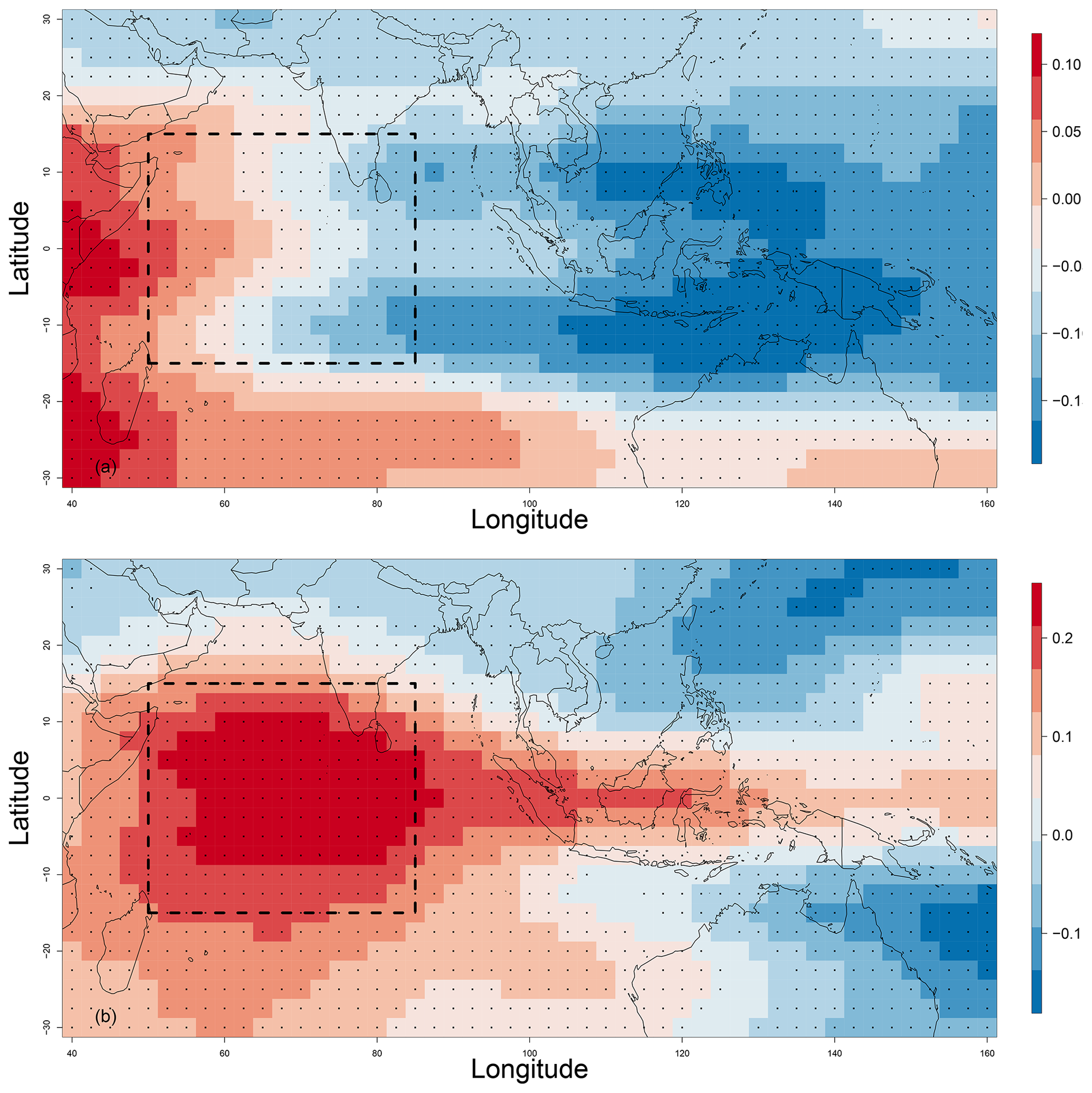
Figure 2The optimal domain of computation of analogs. We computed analogs over the Indian Ocean, in the geographic areas indicated by the dashed black rectangle with coordinates 15∘ S–15∘ N, 50–85∘ E. The figure shows the temporal correlation between Z500, RMM1 (a), and RMM2 (b) for the whole studied period from 1979 to 2020. The correlation is weak, but it is still significant, with p values ≤0.05 that we indicate with black dots over each grid of the considered domain (including the optimal region used to compute analogs).
3.2 Configuration of the stochastic weather generator
The stochastic weather generator (SWG) aims to generate ensembles of random trajectories that yield physically consistent features. Our SWG is based on circulation analogs that are computed in advance with the procedure described in Sect. 3.1 (Yiou, 2014; Krouma et al., 2021). We produce an ensemble hindcast forecast with the circulation analog SWG with the following procedure (see Fig. 3 for a summary).
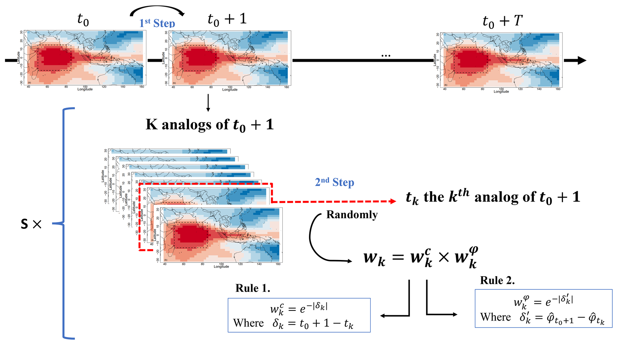
Figure 3Illustration of the SWG process. The first step goes from a given day to the next day. The second step explains how we randomly select a kth analog with respect to weight wk.
For a given day t0 in year y0, we generate a set of S=100 simulations until a time t0+T, where T is the lead time, which goes from 3 to 90 d. We start at day t0 and randomly select an analog (out of K=20) of day t0+1. The random selection of analogs of day t0+1 among K analogs is performed with a weight wk that is computed as the products of two weights, and , defined by the following rules:
-
Weights are inversely proportional to the calendar difference between t0 and analog dates to ensure that time goes “forward”. If δk is the difference in calendar days between t0+1 and tk, where tk is the date of the kth analog of t0+1, then the calendar day sampling weight is proportional to .
-
Weights are the difference between the phase at t0 and analog dates. Indeed, we give more weight to analogs that are in the same phase. If is the difference between and the discrete phase of tk, then the phase weight is proportional to .
Then we set wk=0 when the analog year is y0. Indeed, excluding analog selection in year y0 ensures that we do not use information from the T days that follow t0. Then and the values of wk are normalized so that their sum is 1. Rule 1 is similar to the SWG used by Krouma et al. (2021). Rule 2 adds a constraint to ensure phase consistency across analogs.
We then replace t0 with tk, the selected analog of t0+1, and repeat the operation T times. Hence we obtain a hindcast trajectory between t0 and t0+T. This operation of trajectory simulation from t0 to t0+T is repeated S=100 times. The daily MJO (A(t) or RMMs) of each trajectory is time-averaged between t0 and t0+T. Hence, we obtain an ensemble of S=100 forecasts of the average MJO (A(t) or RMMs) for day t0 and lead time T. Then t0 is shifted by Δt≥1 d, and the ensemble simulation procedure is repeated. This provides a set of ensemble forecasts with analogs.
To evaluate our forecasts, the predictions made with the SWG are compared to the persistence and climatological forecasts. The persistence forecast consists of using the average value between t0−T and t0 for a given year. The climatological forecast takes the climatological mean between t0 and t0+T. The persistence and climatological forecasts are randomized by adding a small Gaussian noise, whose standard deviation is estimated by bootstrapping over T long intervals. We thus generate sets of persistence forecasts and climatological forecasts that are consistent with the observations (Yiou and Déandréis, 2019).
3.3 Forecast verification metrics
We assess the skill of the SWG to forecast the A(t) and the RMMs using two approaches. We start by evaluating the performance of the SWG to forecast A(t). For that, we use probabilistic scores (Zamo and Naveau, 2018; Hersbach, 2000; Marshall et al., 2016) like the continuous ranked probability score (CRPS) for each lead time T. The CRPS is a quadratic measure of the difference between the forecast cumulative distribution function and the empirical cumulative distribution function of the observation (Zamo and Naveau, 2018). The CRPS is defined by
where xa is the observed RMMobs or A(t)obs, P is the cumulative distribution function of x of the ensemble forecast, and ℋ represents the Heaviside function (ℋ(y)=1 if y≥0 and ℋ(y)=0 otherwise). A perfect forecast yields a CRPS value equal to 0.
As the CRPS value depends on the unit of the variable to be predicted, it is useful to normalize it with the CRPS value of a reference forecast, which can be obtained by a persistence or a climatology hypothesis. The continuous ranked probability skill score (CRPSS) is defined as a percentage of improvement over such a reference forecast (Hersbach, 2000). We compute the CRPSS using as a reference the climatology and the persistence.
where is the average of the CRPS of the SWG forecast, and is the average of the CRPS of the reference (either climatology or persistence).
The CRPSS values vary between −∞ and 1. The forecast has improvement over the reference when the CRPSS value is above 0.
We also computed the rank (temporal) correlation between the observations and the median of the 100 simulations (Scaife et al., 2014).
A robust forecast requires a good discrimination skill. A discrimination skill represents the ability to distinguish events from non-events. We measure the skill of the SWG in discriminating between situations leading to the occurrence of an MJO event (active MJO) and those leading to the non-occurrence of the event (inactive MJO). To do so, we use the relative operating characteristic (ROC) score. The ROC is used for binary events (Fawcett, 2006). Since we have a probabilistic forecast, we can use a threshold value of 1 to construct a classifier for the binary event of MJO from the feature A(t):
-
If A(t)≥1 we predict a positive outcome (active MJO).
-
If A(t)<1 we predict a negative outcome (inactive MJO).
The ROC curve is a plot of the success rate versus the false alarm rate (Verde, 2006). The ROC curve could also be a plot of the sensitivity versus the specificity (Fawcett, 2006). The sensitivity (true positive rate) is the probability of an active-MJO event, assuming that A(t)≥1 is really observed. The specificity (true negative rate) refers to the probability of an inactive-MJO event, as long as we have A(t)≤1. Moreover, the sensitivity is a measure of the ability of the prediction to identify true positives, and the specificity is a measure of the ability to identify true negatives. Both quantities describe the accuracy of a prediction that signals the presence or absence of an MJO event (Fawcett, 2006). Therefore, we define the relationship between sensitivity and specificity as follows:
-
means that we have a poor prediction because the rate of true negative and the false alarm rate are the same.
-
means that we have a good prediction.
Another performance measurement that we can infer from the ROC curve is the area under the curve (AUC). The AUC explains how much the forecast model is able to distinguish between binary classes. The AUC is the area in the ROC curve between sensitivity and the false positive rate computed as follows:
where S is the sensitivity, and x is the false positive rate.
An increase in AUC indicates an improvement in discriminatory abilities of the model at predicting a negative outcome as a negative outcome and a positive outcome as a positive outcome. An AUC of 0.5 is non-informative.
Finally, we evaluate the ensemble-mean forecast of RMM1 and RMM2 using the usual scalar metrics for MJO forecasts (Rashid et al., 2011; Silini et al., 2021; Kim et al., 2018). We computed the bivariate anomaly correlation coefficient (COR) and the bivariate root mean square error (RMSE) between the forecasted RMMs () and the observed RMMs () as follows:
where t is the time, T is the lead time of the forecast, and N is the length of the time series (N∼104). We interpret the values of COR and RMSE using thresholds fixed by previous studies to define the forecast skill of the SWG. The forecast has skill when the COR value is larger than 0.5, and the RMSE value is lower than . Rashid et al. (2011) explain that for a climatological forecast, because the standard deviation of the observed RMM indices is 1. Hence, forecasts are considered to be skillful for (i.e., they have lower RMSE than a climatological forecast). We use those thresholds in our analyses.
We compare the RMSE to the ensemble spread in order to evaluate the forecast accuracy. The ensemble spread measures the difference between the members of the ensemble forecast. The ensemble spread ES is obtained by the root mean square difference between the ensemble members and the ensemble mean defined as follows:
where S is the size of the ensemble members, An is the amplitude of the nth ensemble member of the forecast, and is the ensemble average of An over the S members.
We compute the average amplitude error (EA) and the average phase error (Eϕ) for the different lead times T. They allow the evaluation of the quality of the forecast. The average amplitude error (EA) is defined as follows:
The value of EA(T) indicates how fast the forecast system loses the amplitude of the MJO signal. A positive value indicates an overestimation of the amplitude in predictions compared to the observation. A negative value indicates an underestimated amplitude. Rashid et al. (2011) define the average phase error (Eϕ) as
This formulation stems from the ratio of the cross product (numerator) and dot product (denominator) of the vectors of forecasts and observations . Equation (11) is equivalent to the average phase angle difference between the prediction and observations, with a positive angle indicating the forecast leads the observations (Rashid et al., 2011). The negative (positive) value of Eϕ(T) indicates a slower (faster) propagation of the phase in predictions compared to the observations.
We explore the skill of a SWG in forecasting the A(t) and the RMMs (R1 and R2) using analogs of the atmospheric circulation. We generate separately an ensemble of 100 members of the A(t) of the MJO and RMMs using the same approach. The goal is to have a probabilistic forecast of the A(t) for a sub-seasonal lead time T (≈ 2 to 4 weeks). As input to the SWG, we use analogs of the atmospheric circulations. We computed analogs separately from Z500, Z300, the wind at 250 and 850 hPa, and the OLR. We choose to keep analogs from the geopotential at height 500 hPa instead of the other atmospheric fields. We explain our choice in Sect. 5.
Then, we adjusted the geographical region and the window search of analogs (Fig. B1). Indeed, the forecast skill of the MJO depends on the geographical region. We choose to compute the analogs over the Indian Ocean with coordinates of 15∘ S–15∘ N, 50–85∘ E. We argue our choice (i) by the fact that the Indian Ocean corresponds to the first phase of the MJO in the phase-space diagram, where the MJO starts; (ii) because different models found good results by initiating their forecast in this region (Kim et al., 2018); and (iii) based on the experiment analyses that we made over different geographical regions (Fig. B2). We explain that in Appendix B.
We search for analogs within 30 calendar days. This duration corresponds to the life cycle of the MJO. In addition, we adjust the SWG in order to select analogs from the same phase, as described in Sect. 3.2.
To evaluate the skill score of our forecasts, we used two approaches. We used the probabilistic scores such as CRPS, correlation, and ROC score (Sect. 3.3) to evaluate the ensemble forecast of the amplitude. Then, we evaluate the ensembles mean of RMM1 and RMM2. For that, we used scalar metrics such as the COR and the RMSE (Sect. 3.3), as they are commonly used to evaluate MJO forecast (Rashid et al., 2011; Lim et al., 2018).
We show results of the forecast of A(t) and RMMs (R1 and R2) from the analogs of Z500 over the Indian Ocean with a time of search of 30 d. As explained in Sect. 4, we explored the potential of other atmospheric circulations (wind at 250 and 850 hPa, OLR, and Z300) to forecast the MJO amplitude. The forecast skill with analogs of OLR and the zonal wind in the upper and lower troposphere (250 and 850 hPa) was not that satisfying compared to the forecast skill using analogs of Z500 or Z300 (Fig. 4). Indeed, the wind at 250 and 850 hPa and the OLR do not improve the bivariate correlation and RMSE forecast skill of the MJO index for a longer lead time (above 20 d) over Z500 or Z300 (Fig. 4), despite the fact that they are the driver of the MJO. This could be explained by different reasons.
The first reason is related to the composition of the RMM index. Indeed, the OLR is used as a proxy for organized moist convection (Kim et al., 2018). However, the fractional contribution of the convection to the variance of RMMs is considerably lower than the fraction of the zonal wind fields (Kim et al., 2018; Straub, 2013). The second reason is that the MJO predictability can be improved by including atmospheric and oceanic processes (Pegion and Kirtman, 2008). According to some theories that explain the MJO, the geopotential and the moisture are considered to be drivers of precipitation and convection (Zhang et al., 2020). For instance, in the gravity-wave theory for MJO (Yang and Ingersoll, 2013), the convection and precipitation are triggered by a specific geopotential threshold.
Another reason is related to our forecast approach. The composites of OLR and wind speed highly depend on the phase of the MJO (Kim et al., 2018). As our analog approach is constrained by choice of a geographical region, it misses the spatio-temporal variability in OLR and wind speed during the MJO. We computed analogs from other regions (Fig. B1). However, we obtain better forecast scores by focusing on the “small” area represented by a dashed rectangle (Fig. B1). This is explained by the higher quality of analogs.
Indeed, choosing a “large” region to compute analogs yields rather large distances or low correlations for analogs. This implies that the analog SWG gets lower skill scores because the analogs are not very informative. The OLR or zonal wind analogs were computed on the optimal window obtained for Z500 or Z300 as mentioned in Fig. 2, which is not appropriate for OLR or wind speed, as reflected by Kim et al. (2018). Therefore, we find lower COR and RMSE scores compared to the forecast using Z300 and Z500. This is a potential feature of analogs. The analog geometry needs to be imposed a priori in a rather simplistic way, which does not follow the spatio-temporal features of the MJO, which are known independently.
We tested the forecast of A(t) and RMMs using analogs of Z300. We get a satisfactory forecast skill (i.e., with COR>0.5 and ) up to T=60 d. However, we note that the forecast skill scores based on analogs of Z500 are higher for small lead times (up to 30 d). This is explained by the fact that Z300 analogs are close to where the MJO takes place, even if this does not lead to significant improvement over Z500 analog skill scores. Therefore the geopotential heights, although less physically and dynamically relevant for the MJO, are more appropriate predictors from the statistical and mathematical constraints of the analog-based method. The results of the forecast with analogs of Z300 can be found in Appendix A, where we compare the performance of the SWG forecast based on the analogs of Z500 and Z300 for different seasons (Figs. A1 and A2). For those reasons, we decided to keep the results of the forecast for A(t) and RMMs with analogs of Z500. This analysis highlights the capacity of Z500 to catch the variability in the MJO.
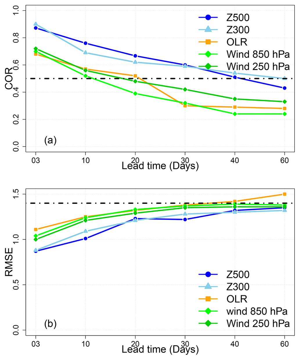
Figure 4COR (a) and RMSE (b) values for different lead times of forecasts from 3 to 60 d over the period from 1979 to 2020 for the SWG forecast using analogs of OLR and zonal wind speed at 250 and 850 hPa as well as Z300 and Z500.
As an illustration, we show the time series of the simulations and observations of the MJO amplitude for 1986. This year yields an unusually large period of RMM amplitude above 1, suggesting an important MJO activity. Figure 5 shows the mean of the 100 simulations and the observations for lead times of 3, 5, and 10 d for the whole year. We find that there is a strong correlation between observed and simulated A(t) for the different lead times represented. Moreover, the SWG was able to distinguish between the active-MJO days (A(t)≥1) and inactive-MJO events (A(t)≤1). The same figures for the forecast with the SWG based on analogs of OLR and Z300 are provided in Appendix A.
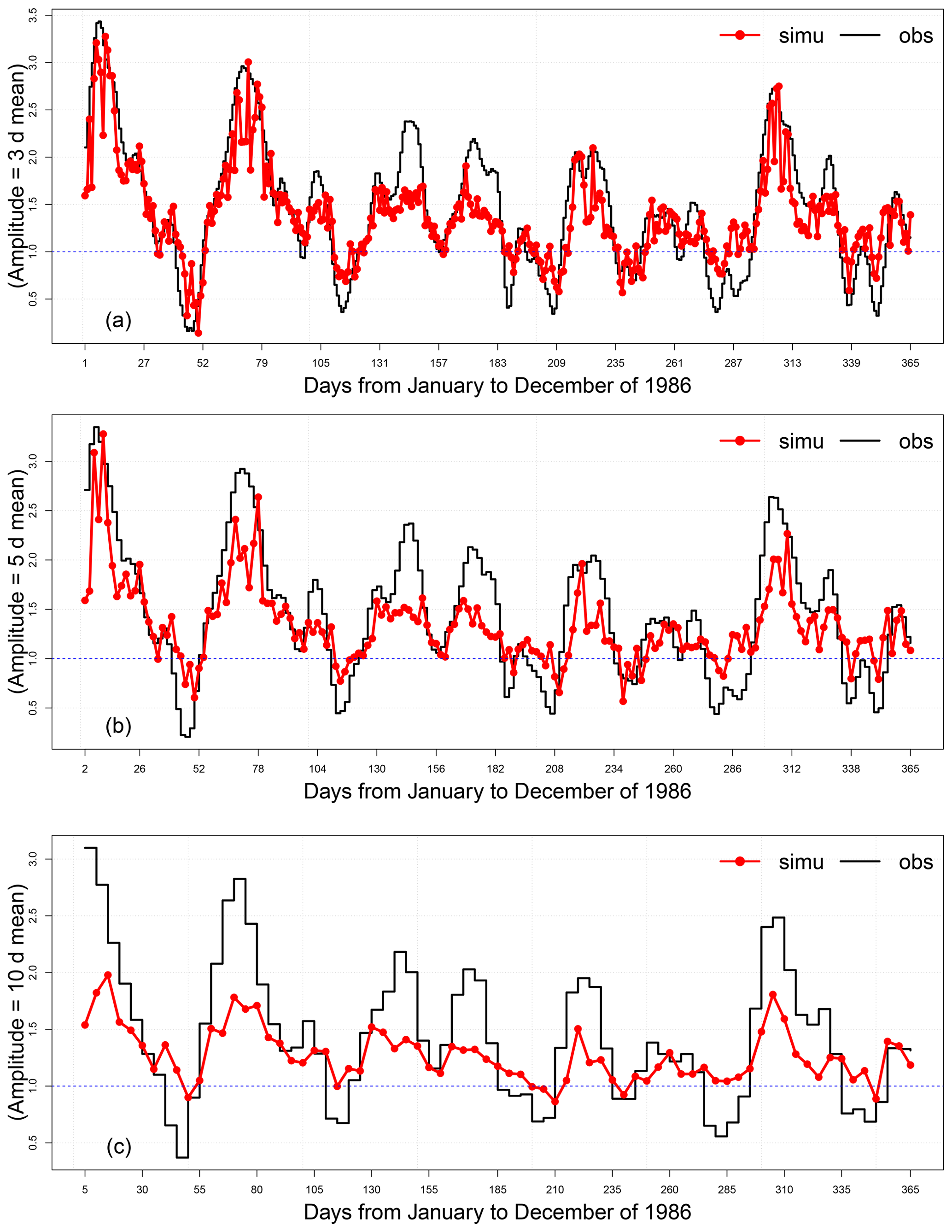
Figure 5Time series of observations and simulations of the MJO amplitude for lead times of 3 (a), 5 (b), and 10 d (c) for the year 1986. The red line represents the mean of the 100 simulations, the black line represents the observations, and the blue line indicates the threshold of the MJO activity (below 1: inactive; above 1: active).
5.1 Evaluation of the ensemble forecast of the MJO amplitude
We evaluate the forecast of amplitude A(t) using the probabilistic skill scores (CRPSS, ROC, and correlation) defined in Sect. 3.3. We consider the average of the skill scores up to each lead time T. In Fig. 6, we show the CRPSS and the correlation for DJF (December, January, and February) and JJA (June, July, and August) for different lead times T going from 3 to 40 d.
The CRPSS was computed using as a reference the forecast made from climatology and persistence. We note that the CRPSS vs. persistence reference decreases with time. It has higher values for d. We note that when the lead time is larger than T=15 d, CRPSS values become stable for both seasons. However, the CRPSS vs. climatology increases with lead time. We note that for small lead times (T≤15 d), the SWG forecast does better than the persistence, while for big lead times T≥15 d, the SWG forecast does better than the climatology. We can say that the forecast has a positive improvement compared to climatology and persistence for DJF and JJA for all the studied lead times. We see that correlation mostly decreases with lead times. The highest correlation is related to small lead times (T≤15 d).
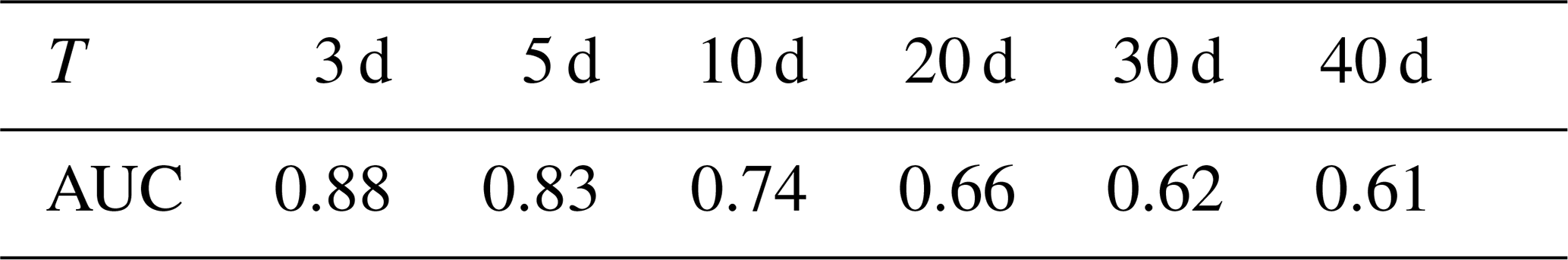
We used the ROC diagram to determine the discrimination between active and inactive events of the MJO. We associated 1 with an active-MJO event and zero with the inactive-MJO events. In Fig. 7, we show the ROC diagram for the different lead times T from 3 to 40 d. Analyzing the AUC, shown in Table 1, we find that until 40 d, the SWG is able to separate non-events (inactive MJO) from events as the AUC values are between 0.88 and 0.61. It is still significant as it is over the diagonal (random forecast). We note that the sensitivity value is 0.9 for 3 d, and it decreases with lead time to reach 0.7 by 40 d. We also find that the specificity and sensitivity are equal for small lead times. However, the specificity remains above ≈0.5 for T=40 d. This value of specificity is still higher than . This indicates that the forecast has skill to distinguish between MJO events until 40 d ahead.
Table 1Area under ROC curve (AUC) for the different lead times T from 3 to 40 d.
Using three probabilistic metrics (CRPSS, correlation, and ROC), we show that the SWG is able to skillfully forecast the MJO amplitude from analogs of Z500. The CRPSS shows a positive improvement of the forecast until 40 d. However, the correlation is significant until 20 d. By using the ROC curve and the discrimination skill, we show that the forecast still has skill until 40 d.
The difference between the lead times that we found using the CRPSS, correlation, and the ROC result from the difference between the skill scores. In fact, the CRPS is used for different categories of events, while the ROC is used for binary events, which is more suitable with our case of study.
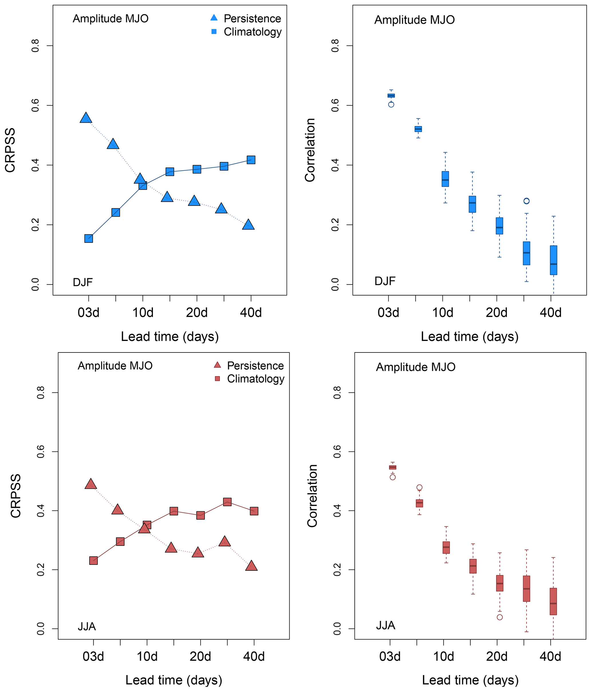
Figure 6Skill scores for the MJO amplitude for lead times going from 3 to 40 d for DJF (blue) and JJA (red) for analogs computed from Z500. Squares indicate CRPSS where the persistence is the reference, triangles indicate CRPSS where the climatology is the reference, and boxplots indicate the probability distribution of correlation between observation and the median of 100 simulations for the period from 1979 to 2020.
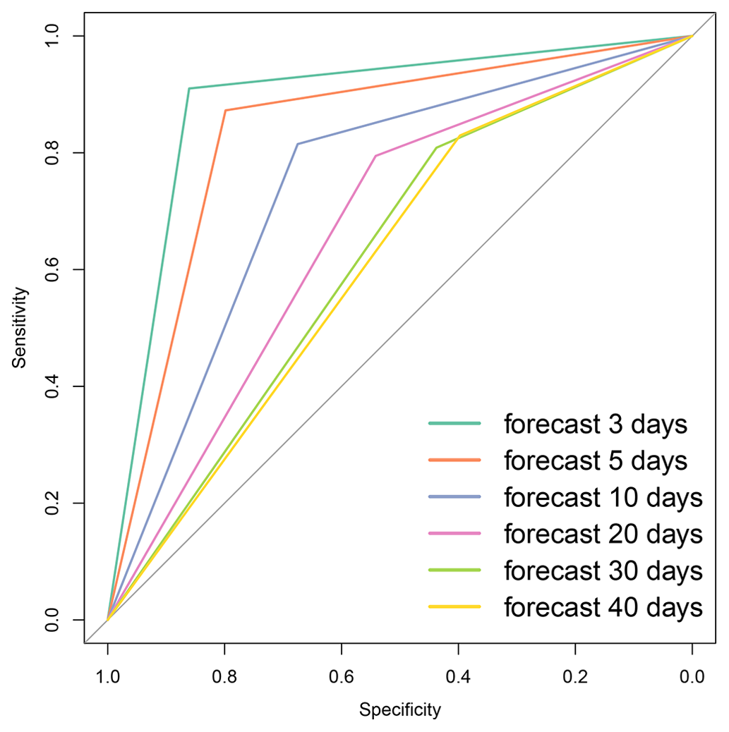
Figure 7ROC curve for all lead times. The plot represents the sensitivity versus the specificity. The diagonal line represents the random classifier obtained when the forecast has no skill. If the ROC curve is below the diagonal line, then the forecast has a poor skill, otherwise it has a good skill; i.e., the forecast has the potential to distinguish between success and false alarms.
5.2 Evaluation of the ensemble-mean forecast of RMMs
In this part, we evaluate the performance of the SWG in forecasting the RMMs (R1 and R2). We simulated R1 and R2 using the SWG and analogs of Z500. Then we used the ensemble mean of R1 and R2 to compute the verification metrics, mainly the COR and RMSE (Rashid et al., 2011; Kim et al., 2018; Silini et al., 2021), as shown in Fig. 8. We looked at COR and RMSE averaged up to each lead time T. Respecting the threshold 0.5 for the COR and for RMSE, we found that the forecast has skill until T=40 d. We have to mention that T values of 60 and 90 d were used for verification purposes.
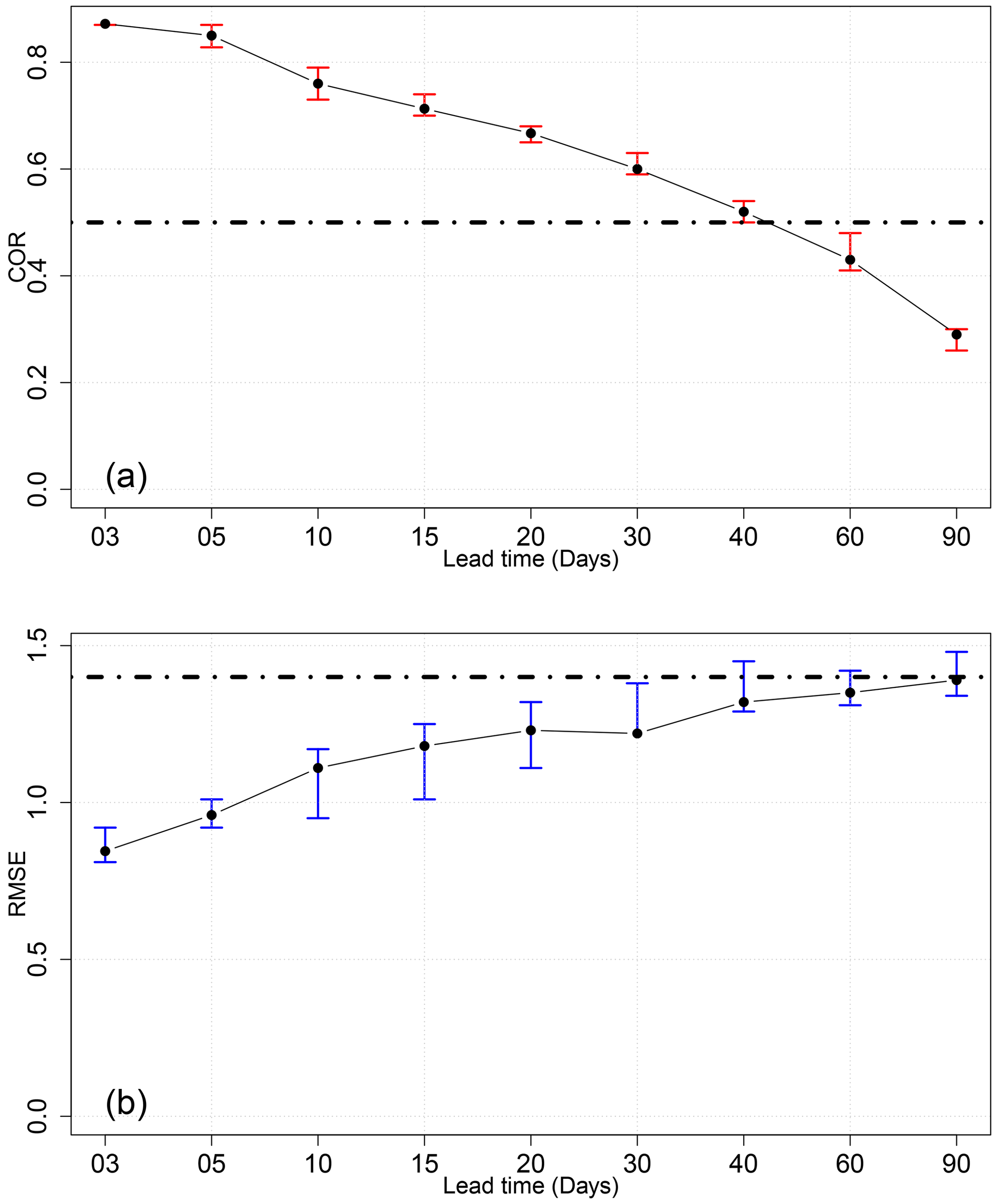
Figure 8The COR (a) and RMSE (b) for the different lead times of forecasts from 3 to 90 d over the period from 1979 to 2020. Confidence intervals are obtained with a bootstrap with 1000 samples.
In order to verify the forecast skill, we computed the ensemble spread, and we compared it to the RMSE values for the different lead times going from 3 to 40 d (Fig. 9). We found that the difference between the ensemble spread and the RMSE increases with lead time. The RMSE is becoming larger with lead time, which indicates that the distance between the observations and simulations is increasing. In addition, the ensemble spread decreases, which indicates that the uncertainties increase with time. This was verified by computing the bias of the forecast, where we could find that it increases with lead time. The bias represents the average bias of RMM1 and RMM2. It was computed between the ensemble mean of the RMMs and the observations of RMMs.
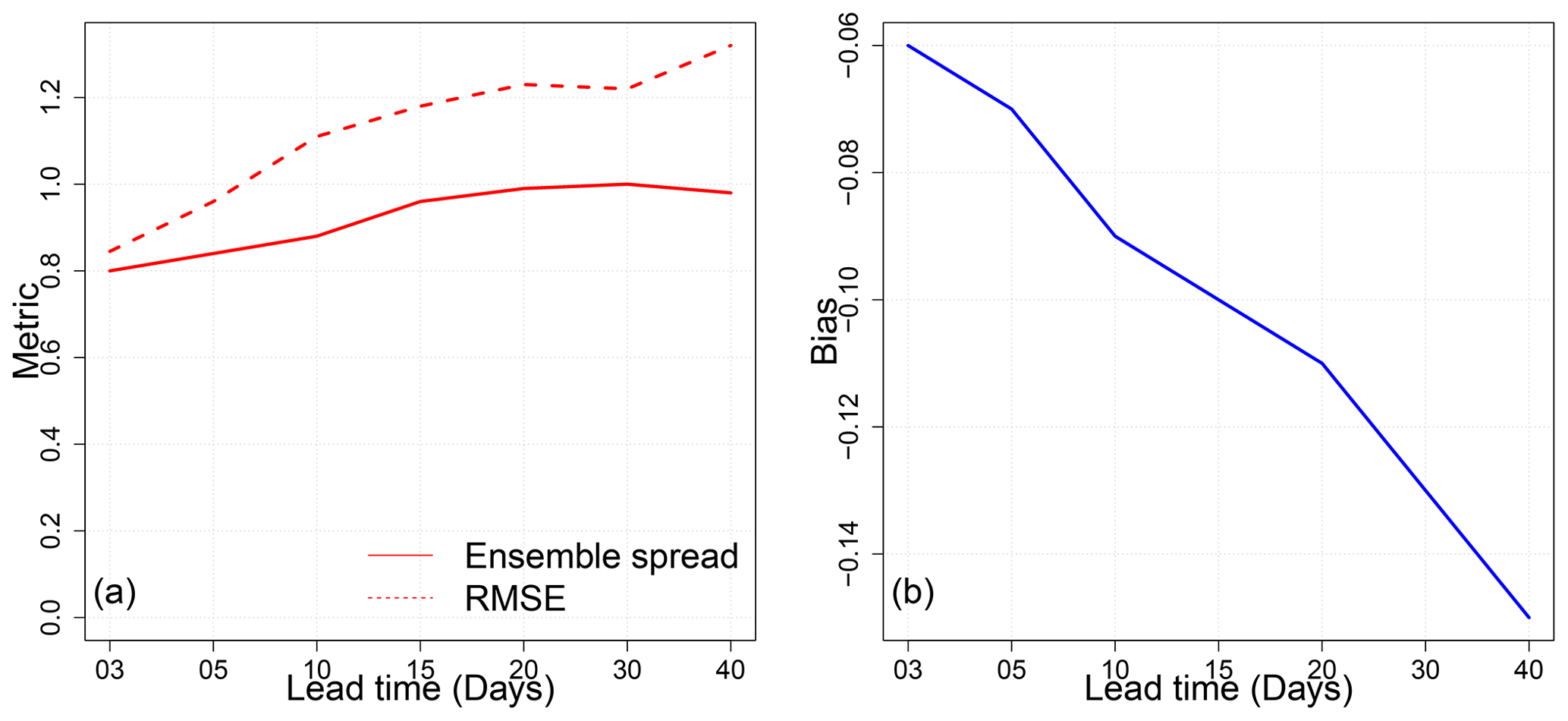
Figure 9(a) Comparison between the ensemble spread and the RMSE. We note that the difference is small for short lead times (≤15 d). “Metric” on the vertical axis refers to ensemble spread and RMSE. (b) The bias between the simulations and the observations for the lead times going from 3 to 40 d.
We explored the sensitivity of the forecast to seasons as shown in Fig. 10. We found that the forecast for DJF and MAM (March, April, May) has a good skill (i.e., with RMSE lower than ) within 30 d. However, for SON (September, October, and November) and JJA, a similar forecast skill was obtained for a lead time of 40 d. The DJF and MAM seasons show the largest RMSE values. This implies that the ensemble forecast in DJFM yields a larger range of values than in SON and JJA, even if the observations and simulations are well correlated. The highest correlation in DJF and MAM could be explained by the fact that the MJO is more active in the boreal winter (DJFM). However, the RMSE values in JJA are more consistent as they represent low distance between simulations and observations. Indeed, even if the MJO events tend to be more intense in DJFM, the amplitude is underestimated. The assessment of the ensemble-mean forecast of RMM1 and RMM2 showed that the forecast has skill until 40 d. However, it is sensitive to seasons, and this is consistent with the previous studies of Wheeler and Hendon (2004), Rashid et al. (2011), and Wu et al. (2016b). Indeed, we found that the SWG forecast of RMM1 and RMM2 has skill, with respect to the thresholds of COR and RMSE, within 40 d for summer (JJA) and 30 d for winter (DJF).
We also computed the amplitude and phase errors (Fig. 11). We found that the EA(t) is negative for all lead times. That indicates a weak amplitude in predictions compared to the observations. The Eϕ(t) is positive until 30 d, which indicates fast propagation of the phase in predictions compared to the observations. Then it becomes negative, which means that the phase is slower. We note that the phase is well predicted, while the amplitude is underestimated (Fig. 11). This is consistent with previous studies (Silini et al., 2021; Rashid et al., 2011).
The assessment of the forecast of MJO amplitude with SWG and analogs of Z500 shows good skill until 40 d using probabilistic scores (CRPSS vs. climatology is 0.2, and CRPSS vs. persistence is 0.4) and scalar scores (COR=0.54 and RMSE=1.30) as explained in Sects. 5.1 and 5.2. The SWG forecast shows a positive improvement compared to the climatology and the persistence within 40 d (Fig. 6). In addition, the ROC curve confirmed the ability of the SWG forecast to distinguish between the active and inactive-MJO amplitude as shown in Fig. 7. The same result was obtained using the ensemble mean of RMM1 and RMM2 as represented in Fig. 8. The SWG forecast of RMM1 and RMM2 has good skill within 30–4 d, respecting the threshold of 0.5 for the COR and for RMSE. The difference in the lead time of the forecast depends on the seasons as represented in Fig. 10. This is consistent with Wu et al. (2016a), Wheeler and Weickmann (2001), and Rashid et al. (2011), who found significant differences in skill scores between seasons. We find that the forecast has skill until 30 d for DJF and MAM (with ) and 40 d for JJA and SON (with COR=0.5) as shown in Fig. 10. This is different from Rashid et al. (2011) and Silini et al. (2021), who obtain higher forecast skill in the winter. However, it is consistent with the results of Wu et al. (2016b) and Vitart (2017), who found higher skill scores for JJA.
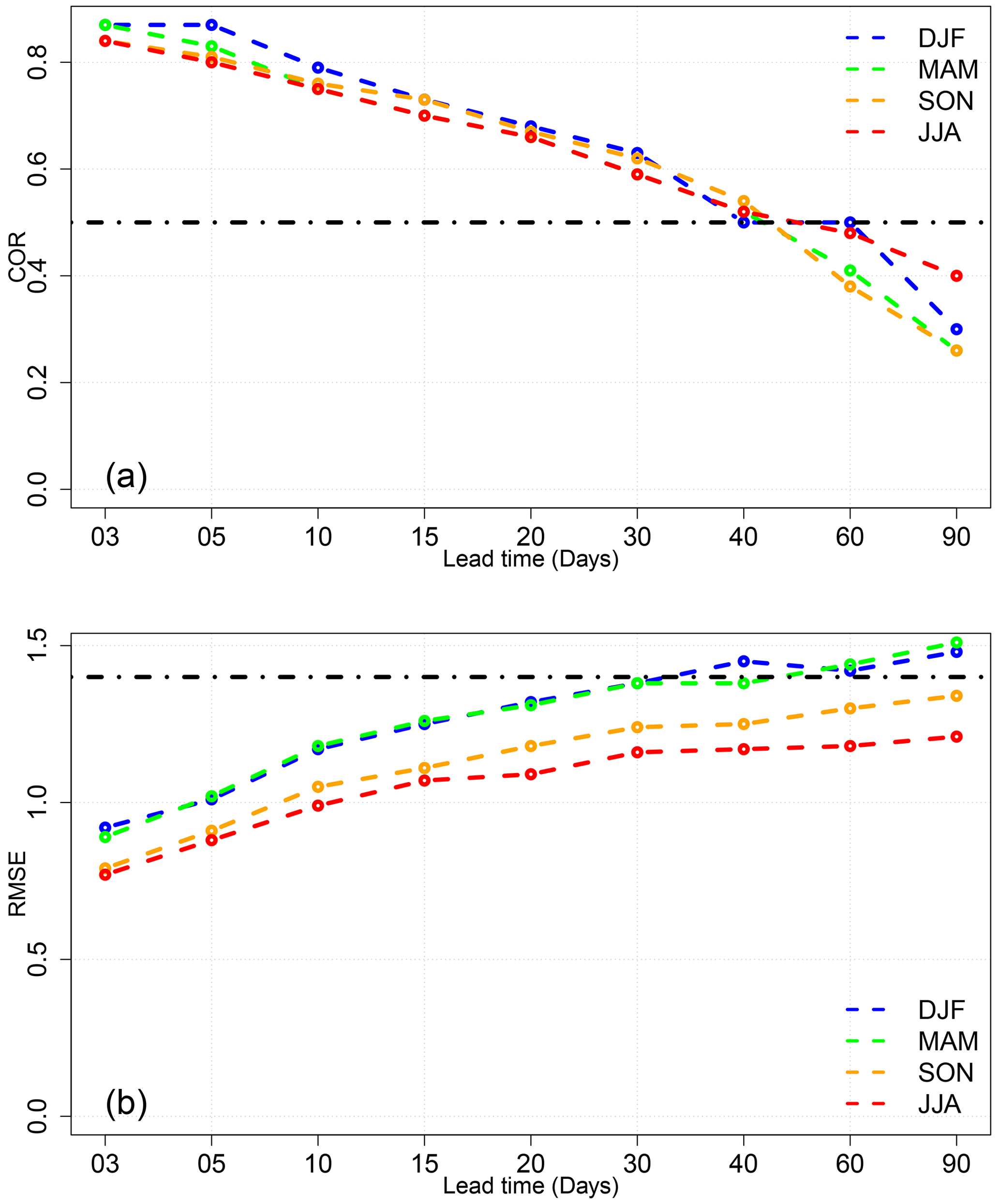
Figure 10The COR (a) and RMSE (b) for the different lead times of forecasts from 3 to 90 d over the period from 1979 to 2020 for the different seasons DJF, JJA, MAM, and SON.
We assessed the forecast skill of the SWG with other forecasts. We selected two models, POAMA (the Australian Bureau of Meteorology coupled ocean–atmosphere seasonal prediction system) and the ECMWF model, which provide probabilistic and deterministic forecast of the MJO, respectively. We compared mainly the maximum lead time of the MJO amplitude forecast. The POAMA model provides a 10-member ensemble. In hindcast mode, the POAMA model has skill up to 21 d (Rashid et al., 2011). The ECMWF reforecasts with Cycle 46r1 have skill to around 40 d. For the error in the amplitude and phase, we found that the ECMWF reforecasts shows lower average amplitude and phase errors compared to those from the SWG forecasts. However, what we found is consistent with other dynamical models (Kim et al., 2018) where they overestimate or underestimate the amplitude and the phase of the MJO.
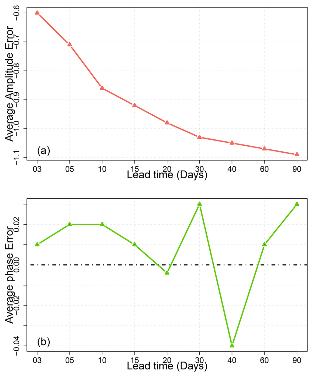
Figure 11The average amplitude error (EA) and average phase error (Eϕ) of the MJO over all seasons for the period from 1979 to 2020. We note that the amplitude is underestimated, and the phase is well predicted by comparing predictions to forecasts.
In addition, we compared quantitatively the SWG forecast with the ECMWF forecast (Fig. 12). The ECMWF reforecasts were taken from Silini et al. (2022). We found that the ECMWF forecast has the highest correlation until 20 d compared to the SWG forecast. The RMSE values of the ECMWF forecast are always small compared to the SWG forecast, which indicates a good reliability skill of the ECMWF forecast for lead times of 5 and 10 d. However, for lead times of 20 d the RMSE of the ECMWF forecast coincides with the RMSE of the SWG, which shows the improvement of the SWG forecast to lead times above 20 d. The skill scores of the ECMWF (COR and RMSE) (Silini et al., 2022) are computed for each lead time, which is different from our way of computing the skill score (considering the average lead time). Of course, this comparison was made to check the performance of our forecast and not to say that the SWG model can replace a numerical prediction.
We also compared the SWG forecast skill with a machine learning forecast of MJO indices (RMM1 and RMM2) (Silini et al., 2021). Silini et al. (2021) explored the skill forecast of two artificial neural network types, FFNN (feed-forward neural network) and AR-RNN (autoregressive recurrent neural network), on MJO indices. Silini et al. (2021) found that the machine learning method gives good skill scores until 26–27 d with respect to the standard thresholds of COR and RMSE. We compared the skill scores (RMSE and COR) of the SWG and Silini et al. (2021) forecasts for all lead times. We found that the two models have the same correlation until 10 d. After 10 d, the correlation of Silini et al. (2021) forecasts decreases rapidly, while the correlation of SWG is still significant. For the RMSE, we found that the SWG has smaller values for a lead time of 10 d. This indicates that the SWG forecast is more reliable. However, from 30 d, the RMSE of the two models starts to be the same.
To sum up, the comparison of SWG forecasts to ECMWF and Silini et al. (2021) forecasts shows that for small lead times (up to 10 d) the ECMWF forecast has better skill. However, the SWG shows a positive improvement for long lead times.
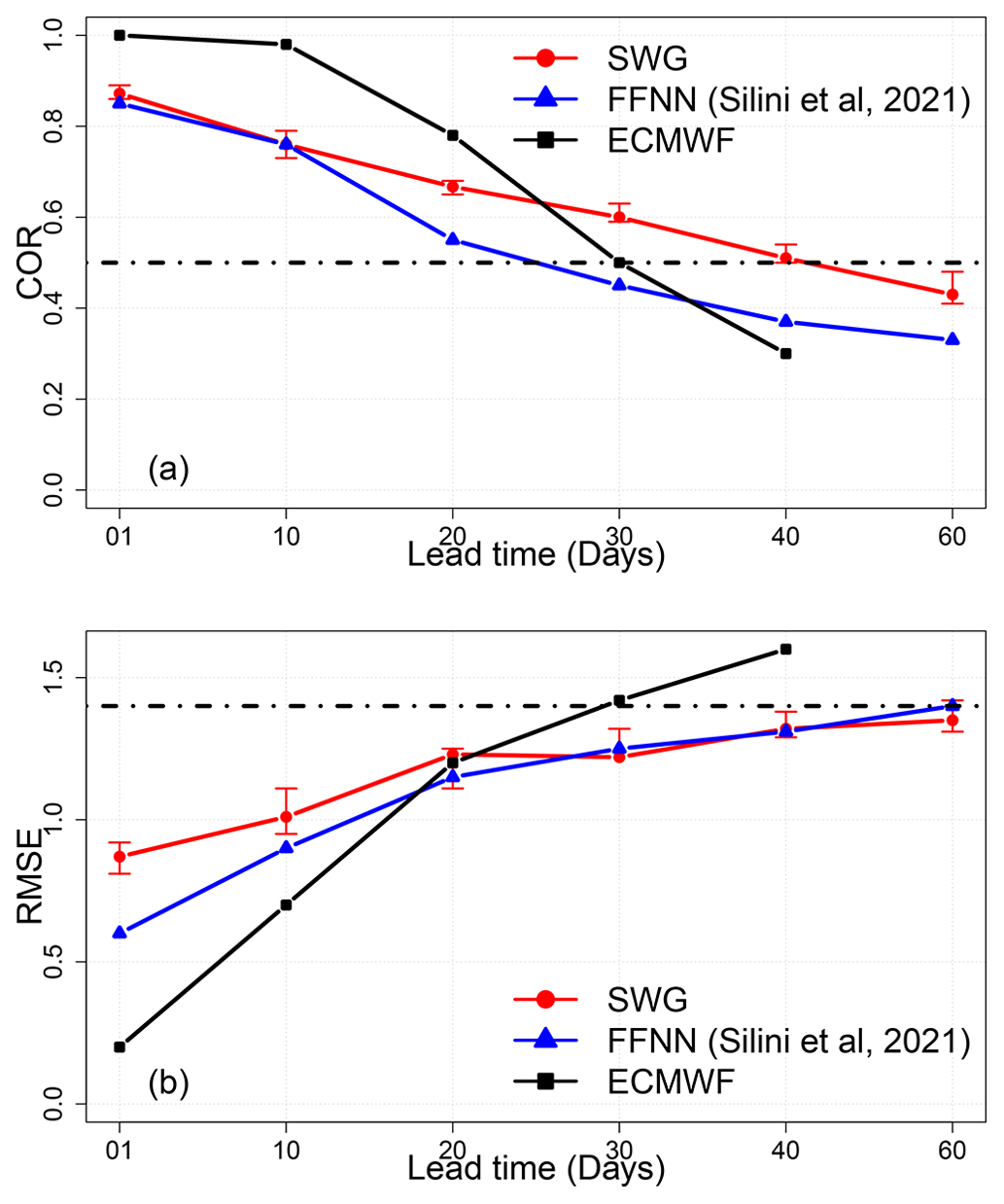
Figure 12Comparison of the values of COR (a) and RMSE (b) between the SWG forecast and forecasts of Silini et al. (2021) (blue lines) and the ECMWF (black lines). Confidence intervals for SWG (red lines) were obtained with a bootstrap procedure over the simulations (1000 samples).
We performed an ensemble forecast of the MJO amplitude using analogs of the atmospheric circulation and a stochastic weather generator. We used the Z500 as a driver of the circulation (Fig. 4) over the Indian Ocean (Fig. 2), and we considered analogs from the same phase to provide the forecast for the sub-seasonal lead time. We explored two ways to forecast the MJO, starting by directly forecasting the daily amplitude, then the daily MJO indices, RMM1 and RMM2, from 1979 to 2020.
We assessed the forecast skill of the MJO forecast by evaluating the ensemble member and the mean of the ensemble member using probabilistic and scalar verification methods, respectively. This allowed us to evaluate the forecast and also to explore the difference between the two verification methods.
We used probabilistic skill scores as the CRPSS and the AUC of the ROC curve (Table 1). We found that the forecast showed positive improvement over the persistence and the climatology within 40 d (CRPSS; Fig. 6). The SWG forecast of the MJO amplitude also showed the capacity to distinguish between active and inactive MJO (ROC curve; Fig. 7) for the different lead times. Using the scalar scores (COR and RMSE) and the ensemble mean of the forecast of RMM1 and RMM2, we found that the SWG is able to forecast the MJO indices (RMM1 and RMM2) within 30–40 d.
We found that the forecast is sensitive to seasons (Fig. 10). The forecast has skill up to 30 d for the boreal winter (DJF and MAM), while it goes to 40 d for the boreal summer (JJA) and SON. That was consistent with previous studies (Silini et al., 2021; Rashid et al., 2011; Vitart et al., 2017). We also note that the forecast of the phase is better than of the amplitude according to the errors for amplitude and phase (Fig. 11). Finally, we found that the SWG had improvement over the ECMWF forecast for long lead times (T>30 d) and a machine learning forecast (Silini et al., 2021) forecast for lead times T>20 d.
This paper hence confirms the skill of the SWG in generating ensembles of MJO index forecasts from analogs of circulation. Such information would be useful to forecast impact variables such as precipitation and temperature.
We did the forecast of RMM1 and RMM2 using analogs of Z300 (Fig. A4), OLR (Fig. A3), and the zonal wind at 250 and 850 hPa (Fig. 4). The aim of using different atmospheric fields to compute analogs is to choose the analog circulation for the MJO forecast with the SWG as explained previously in Sect. 4. We found that the SWG based on analogs of Z300 yields good skills (COR>0.5 and ) within T=60 d (Fig. 4). However, the skill of the forecast is better for small lead times ≤30 d with analogs of Z500 (Fig. 4). We checked the sensitivity of the forecast to seasons as illustrated in Figs. A1 and A2 using separate analogs of Z500 and Z300. We compared the COR and the RMSE for different lead times (Figs. A1 and A2). We found that the RMSE values for the SWG forecast based on analogs of Z300 are the same as the forecast from analogs of Z500 for the different seasons and at different lead times (Fig. A2). The RMSE for SON and JJA is lower than the threshold for the T from 3 to 90 d for both forecasts (Fig. A2). However, for DJF and MAM the SWG forecast reaches the threshold of at 37 d with analogs of Z300, which is slightly higher than the maximum lead time with Z500 (Fig. A2). The COR is slightly higher with analogs of Z500 at different lead times (Fig. A1). However, the threshold of 0.5 is exceeded with forecasts based on analogs of Z300 (Fig. A1).
In this part, we also show the time series for the forecast at different lead times d for the same year (1986) for the SWG forecast with analog circulation computed from OLR (Fig. A3) and from Z300 (Fig. A4). We note that the correlation between the mean of the simulations (red line) and the observations of the MJO amplitude are better correlated with SWG forecasts based on analogs of Z300 (Fig. A4) than the one based on analogs of OLR (Fig. A3).
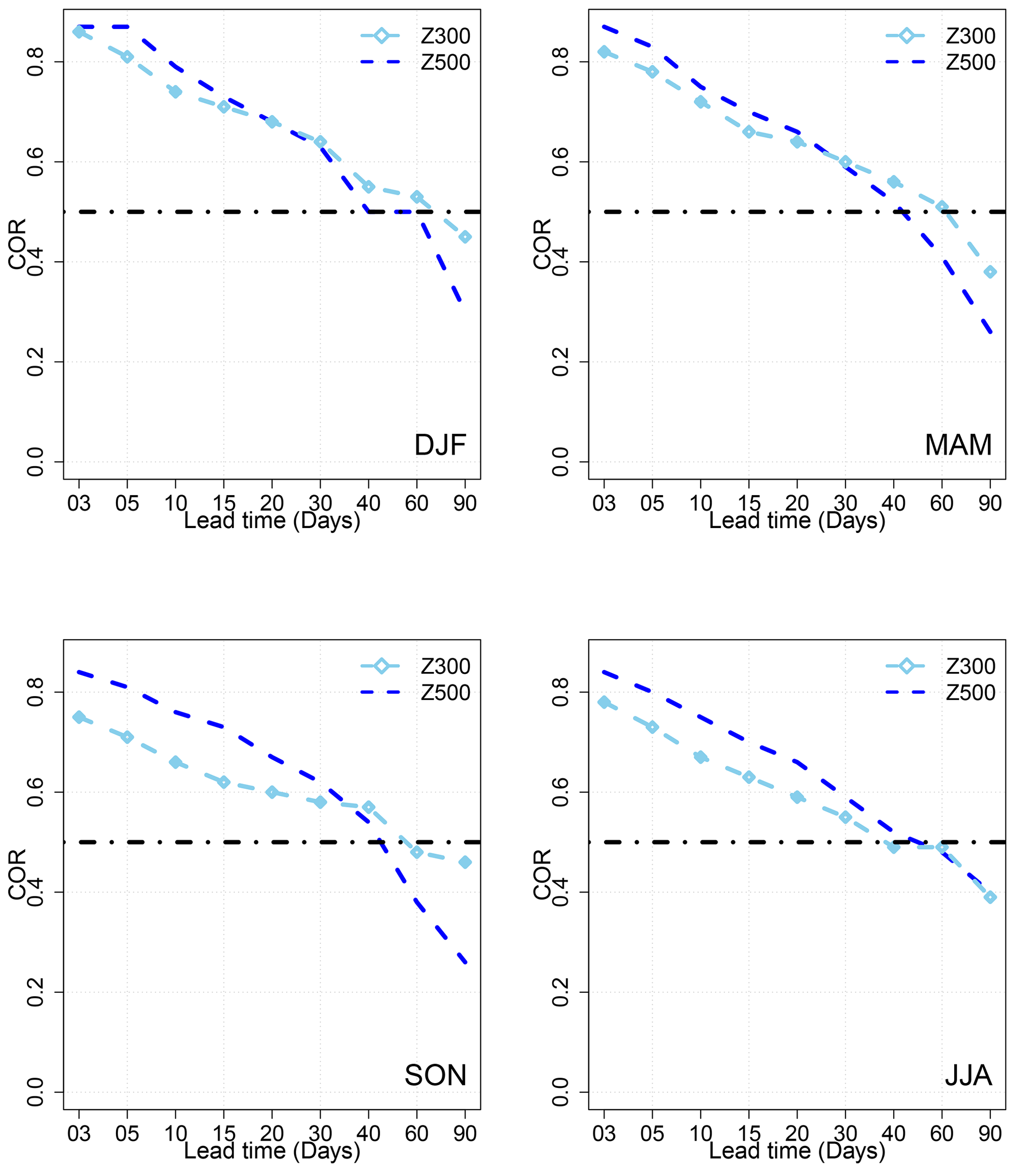
Figure A1COR values for different lead times of forecasts from 3 to 90 d over the period from 1979 to 2020 for the SWG forecast based on analogs of Z500 and Z300 for different seasons (DJF, JJA, MAM, and SON).
Figure A2RMSE values for different lead times of forecasts from 3 to 90 d over the period from 1979 to 2020 for the SWG forecast based on analogs of Z500 and Z300 for different seasons (DJF, JJA, MAM, and SON).
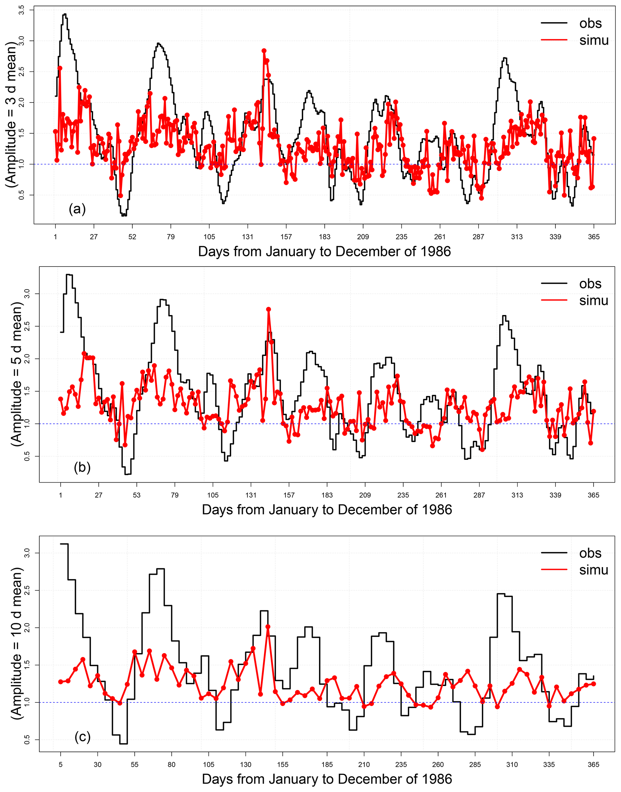
Figure A3Time series of observations and simulations of the MJO amplitude computed from analogs of OLR for lead times of 3 (a), 5 (b), and 10 d (c) for the year 1986. The red line represents the mean of the 100 simulations, the black line represents the observations, and the blue line indicates the threshold of the MJO activity A(t)>1.

Figure A4Time series of observations and simulations of the MJO amplitude computed from analogs of Z300 for lead times of 3 (a), 5 (b), and 10 d (c) for the year 1986. The red line represents the mean of the 100 simulations, the black line represents the observations, and the blue line indicates the threshold of the MJO activity A(t)>1.
We show in Fig. B2 the bivariate correlation (COR) and the RMSE from different geographical regions that we represent in Fig. B1. The different geographical regions shown in Fig. B2 were used to adjust the geographical region to compute analogs.
The COR reaches the threshold of 0.5 at T=40 d for the geographical region with coordinates of 15∘ S–15∘ N, 50–85∘ E (Fig. B2). The same result is found for the region with coordinates of 15∘ S–15∘ N, 60–120∘ E (light-blue line in Fig. B2). However, the COR is lower for the other lead times d compared to the one for the region (15∘ S–15∘ N, 50–85∘ E). For the region with the coordinates (15∘ S–15∘ N, 85–120∘ E), the threshold of 0.5 for the COR is obtained at a lead time of 34 d (green line in Fig. B2). For the region with coordinates (15∘ S–15∘ N, 90–150∘ E), the forecast skill is significant with COR 0.5, at T=30 d (orange line in Fig. B2), which remains the same results for this region compared to (Silini et al., 2022). The RMSE for the different regions is quite the same (Fig. B2), even if the values for the region (15∘ S–15∘ N, 50–85∘ E) are slightly lower within 30 d. Therefore the skill forecast (using the bivariate correlation and the RMSE) remains higher for the considered geographical region with the coordinates (15∘ S–15∘ N, 50–85∘ E).
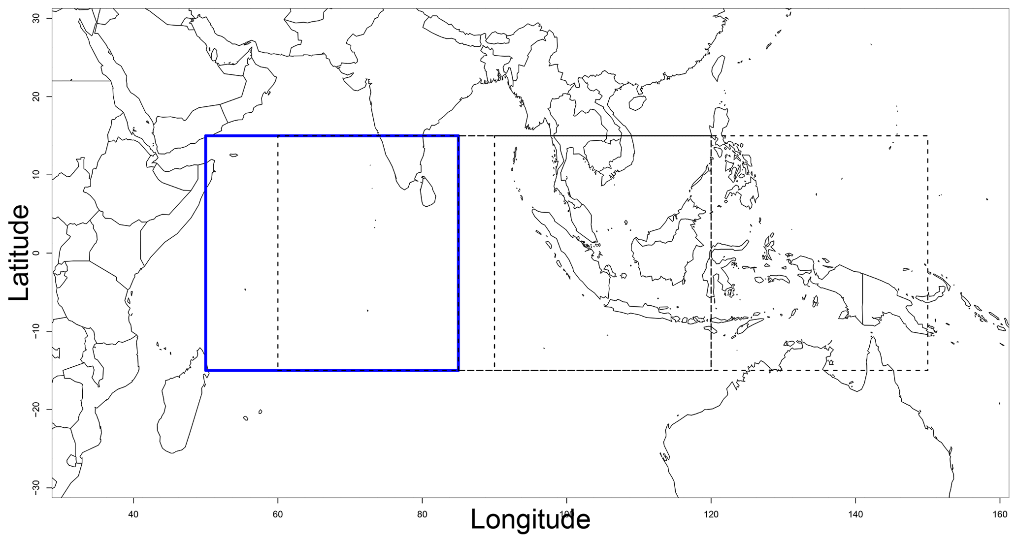
Figure B1Domains of computation of analogs. We computed analogs over the Indian Ocean with coordinates 15∘ S–15∘ N, 50–85∘ E (blue rectangle); the Indian and Pacific oceans with coordinates 15∘ S–15∘ N, 85–120∘ E; and the Indian Ocean–Maritime Continent region with coordinates 15∘ S–15∘ N, 90–150∘ E.
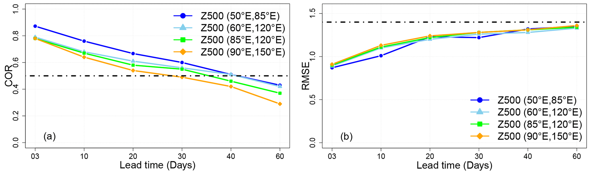
Figure B2Comparison between the COR (a) and RMSE (b) of the SWG forecast based on analogs of Z500 computed over different geographical regions, for lead times going from 3 to 60 d over the period from 1979 to 2020. The forecast was made with analogs computed over the Indian Ocean with coordinates 15∘ S–15∘ N, 50–85∘ E, and 15∘ S–15∘ N, 60–120∘ E; the Indian and Pacific oceans with coordinates 15∘ S–15∘ N, 85–120∘ E; and the Indian Ocean–Maritime Continent region with coordinates 15∘ S–15∘ N, 90–150∘ E. As the latitude is the same for the different considered geographical regions, we just mention the longitude of each domain in the legend.
We checked the dependence of the SWG forecast skill of the amplitude of the MJO and the MJO phases. We verified the relationship between the CRPS at T=5 d and the MJO phases (Fig. C1). We divided the CRPS values in two classes:
As shown in Fig. C1 the difference between the boxplots in the two cases is smaller. Hence, we can say that the dependence of the forecast skill of the MJO amplitude with SWG and the MJO phases is small.
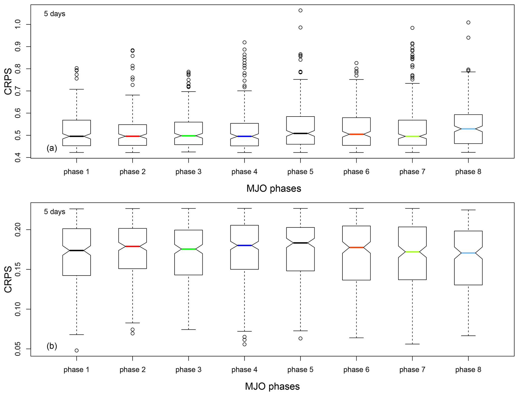
Figure C1Relationship between CRPS and MJO phases. (a) CRPS values above the 75th quantile and (b) CRPS values above the 25th quantile.
The code and data files are available at http://doi.org/10.5281/zenodo.4524562 (Krouma, 2021).
MK designed and performed the analyses and wrote the manuscript. PY co-designed the analyses. RS provided data for comparison.
The contact author has declared that none of the authors has any competing interests.
Publisher’s note: Copernicus Publications remains neutral with regard to jurisdictional claims in published maps and institutional affiliations.
This work is part of the EU International Training Network (ITN) Climate Advanced Forecasting of sub-seasonal Extremes (CAFE). The project receives funding from the European Union’s Horizon 2020 research and innovation program under the Marie Skłodowska-Curie Actions (grant agreement no. 813844). The authors would like to thank Alvaro Corral and Monica Minjares for the discussions.
This research has been supported by the Horizon 2020.
This paper was edited by Yun Liu and reviewed by two anonymous referees.
Ailliot, P., Allard, D., Monbet, V., and Naveau, P.: Stochastic weather generators: an overview of weather type models, Journal de la Société Française de Statistique, p. 15, http://www.numdam.org/item/JSFS_2015__156_1_101_0/ (last access: 22 December 2022), 2015. a
Atencia, A. and Zawadzki, I.: A comparison of two techniques for generating nowcasting ensembles, Part I: Lagrangian ensemble technique, Month. Weather Rev., 142, 4036–4052, 2014. a
Barlow, M., Zaitchik, B., Paz, S., Black, E., Evans, J., and Hoell, A.: A Review of Drought in the Middle East and Southwest Asia, J. Climate, 29, 8547–8574, https://doi.org/10.1175/JCLI-D-13-00692.1, 2016. a
Becker, E. J., Berbery, E. H., and Higgins, R. W.: Modulation of Cold-Season U.S. Daily Precipitation by the Madden-Julian Oscillation, J. Climate, 24, 5157–5166, https://doi.org/10.1175/2011JCLI4018.1, 2011. a
Blanchet, J., Stalla, S., and Creutin, J.-D.: Analogy of multiday sequences of atmospheric circulation favoring large rainfall accumulation over the French Alps, Atmos. Sci. Lett., 19, e809, https://doi.org/10.1002/asl.809, 2018. a
Cassou, C.: Intraseasonal interaction between the Madden-Julian Oscillation and the North Atlantic Oscillation, Nature, 455, 523–527, https://doi.org/10.1038/nature07286, 2008. a
Fawcett, T.: An introduction to ROC analysis, Pattern Recogn. Lett., 27, 861–874, https://doi.org/10.1016/j.patrec.2005.10.010, 2006. a, b, c
Grimit, E. P. and Mass, C. F.: Initial Results of a Mesoscale Short-Range Ensemble Forecasting System over the Pacific Northwest, Weather Forecast., 17, 192–205, https://doi.org/10.1175/1520-0434(2002)017<0192:IROAMS>2.0.CO;2, 2002. a
Hersbach, H.: Decomposition of the Continuous Ranked Probability Score for Ensemble Prediction Systems, Weather Forecast., 15, 559–570, https://doi.org/10.1175/1520-0434(2000)015<0559:DOTCRP>2.0.CO;2, 2000. a, b
Hersbach, H., Bell, B., Berrisford, P., Hirahara, S., Horányi, A., Muñoz-Sabater, J., Nicolas, J., Peubey, C., Radu, R., and Schepers, D.: The ERA5 global reanalysis, Q. J. Roy. Meteor. Soc., 146, 1999–2049, 2020. a
IRI: The University of Columbia (USA) – RMMs data, https://iridl.ldeo.columbia.edu/SOURCES/.BoM/.MJO/, last access: 19 December 2022. a
Kim, H., Vitart, F., and Waliser, D. E.: Prediction of the Madden-Julian Oscillation: A Review, J. Climate, 31, 9425–9443, https://doi.org/10.1175/JCLI-D-18-0210.1, 2018. a, b, c, d, e, f, g, h, i, j
Kistler, R., Kalnay, E., Collins, W., Saha, S., White, G., Woollen, J., Chelliah, M., Ebisuzaki, W., Kanamitsu, M., Kousky, V., van den Dool, H., Jenne, R., and Fiorino, M.: The NCEP-NCAR 50-year reanalysis: Monthly means CD-ROM and documentation, B. Am. Meteorol. Soc., 82, 247–267, 2001. a
Krouma, M.: Assessment of stochastic weather forecast based on analogs of circulation, Zenodo [code, data set], https://doi.org/10.5281/zenodo.4524562, 2021. a
Krouma, M., Yiou, P., Déandreis, C., and Thao, S.: Assessment of stochastic weather forecast of precipitation near European cities, based on analogs of circulation, Geosci. Model Dev., 15, 4941–4958, https://doi.org/10.5194/gmd-15-4941-2022, 2022. a, b, c, d, e, f, g
Lafleur, D. M., Barrett, B. S., and Henderson, G. R.: Some Climatological Aspects of the Madden-Julian Oscillation (MJO), J. Climate, 28, 6039–6053, https://doi.org/10.1175/JCLI-D-14-00744.1, 2015. a, b, c, d
Lim, Y., Son, S.-W., and Kim, D.: MJO Prediction Skill of the Subseasonal-to-Seasonal Prediction Models, J. Climate, 31, 4075–4094, https://doi.org/10.1175/JCLI-D-17-0545.1, 2018. a, b, c
Lin, H., Brunet, G., and Derome, J.: Forecast Skill of the Madden-Julian Oscillation in Two Canadian Atmospheric Models, Mon. Weather Rev., 136, 4130–4149, https://doi.org/10.1175/2008MWR2459.1, 2008. a
Lorenz, E. N.: Atmospheric Predictability as Revealed by Naturally Occurring Analogues, J. Atmos. Sci., 26, 636–646, 1969. a
Marshall, A. G., Hendon, H. H., and Hudson, D.: Visualizing and verifying probabilistic forecasts of the Madden-Julian Oscillation: PROBABILISTIC MJO FORECASTS, Geophys. Res. Lett., 43, 12278–12286, https://doi.org/10.1002/2016GL071423, 2016. a
Palmer, T. N.: Predicting uncertainty in forecasts of weather and climate, Rep. Prog. Phys., 63, 71–116, 2000. a
Pegion, K. and Kirtman, B. P.: The Impact of Air-Sea Interactions on the Predictability of the Tropical Intraseasonal Oscillation, J. Climate, 21, 5870–5886, https://doi.org/10.1175/2008JCLI2209.1, 2008. a
Platzer, P., Yiou, P., Naveau, P., Filipot, J.-F., Thiébaut, M., and Tandeo, P.: Probability Distributions for Analog-To-Target Distances, J. Atmos. Sci., 78, 3317–3335, https://doi.org/10.1175/JAS-D-20-0382.1, 2021. a
Rashid, H. A., Hendon, H. H., Wheeler, M. C., and Alves, O.: Prediction of the Madden-Julian oscillation with the POAMA dynamical prediction system, Clim. Dynam., 36, 649–661, https://doi.org/10.1007/s00382-010-0754-x, 2011. a, b, c, d, e, f, g, h, i, j, k, l, m, n
Scaife, A. A., Arribas, A., Blockley, E., Brookshaw, A., Clark, R. T., Dunstone, N., Eade, R., Fereday, D., Folland, C. K., and Gordon, M.: Skillful long-range prediction of European and North American winters, Geophys. Res. Lett., 41, 2514–2519, 2014. a
Silini, R., Barreiro, M., and Masoller, C.: Machine learning prediction of the Madden-Julian oscillation, npj Clim. Atmos. Sci., 4, 57, https://doi.org/10.1038/s41612-021-00214-6, 2021. a, b, c, d, e, f, g, h, i, j, k, l, m, n
Silini, R., Lerch, S., Mastrantonas, N., Kantz, H., Barreiro, M., and Masoller, C.: Improving the prediction of the Madden-Julian Oscillation of the ECMWF model by post-processing, EGUsphere [preprint], https://doi.org/10.5194/egusphere-2022-2, 2022. a, b, c
Sivillo, J. K., Ahlquist, J. E., and Toth, Z.: An ensemble forecasting primer, Weather Forecast., 12, 809–818, 1997. a
Stachnik, J. P. and Chrisler, B.: An index intercomparison for MJO events and termination, J. Geophys. Res.-Atmos., 125, https://doi.org/10.1029/2020JD032507, e2020JD032507, 2020. a
Straub, K. H.: MJO Initiation in the Real-Time Multivariate MJO Index, J. Climate, 26, 1130–1151, https://doi.org/10.1175/JCLI-D-12-00074.1, 2013. a, b
Toth, Z. and Kalnay, E.: Ensemble forecasting at NCEP and the breeding method, Mon. Weather Rev., 125, 3297–3319, 1997. a
Ventrice, M. J., Wheeler, M. C., Hendon, H. H., Schreck, C. J., Thorncroft, C. D., and Kiladis, G. N.: A Modified Multivariate Madden-Julian Oscillation Index Using Velocity Potential, Mon. Weather Rev., 141, 4197–4210, https://doi.org/10.1175/MWR-D-12-00327.1, 2013. a, b
Verde, M. F.: Measures of sensitivity based on a single hit rate and false alarm rate: The accuracy, precision, and robustness of “Az, and A”, Percept. Psychophys., 68, 643–654, 2006. a
Vitart, F.: Madden-Julian Oscillation prediction and teleconnections in the S2S database, Q. J. Roy. Meteor. Soc., 143, 2210–2220, https://doi.org/10.1002/qj.3079, 2017. a
Vitart, F., Ardilouze, C., Bonet, A., Brookshaw, A., Chen, M., Codorean, C., Déqué, M., Ferranti, L., Fucile, E., Fuentes, M., Hendon, H., Hodgson, J., Kang, H.-S., Kumar, A., Lin, H., Liu, G., Liu, X., Malguzzi, P., Mallas, I., Manoussakis, M., Mastrangelo, D., MacLachlan, C., McLean, P., Minami, A., Mladek, R., Nakazawa, T., Najm, S., Nie, Y., Rixen, M., Robertson, A. W., Ruti, P., Sun, C., Takaya, Y., Tolstykh, M., Venuti, F., Waliser, D., Woolnough, S., Wu, T., Won, D.-J., Xiao, H., Zaripov, R., and Zhang, L.: The Subseasonal to Seasonal (S2S) Prediction Project Database, B. Am. Meteorol. Soc., 98, 163–173, https://doi.org/10.1175/BAMS-D-16-0017.1, 2017. a
Wheeler, M. and Weickmann, K. M.: Real-Time Monitoring and Prediction of Modes of Coherent Synoptic to Intraseasonal Tropical Variability, Mon. Weather Rev., 129, 2677–2694, https://doi.org/10.1175/1520-0493(2001)129<2677:RTMAPO>2.0.CO;2, 2001. a
Wheeler, M. C. and Hendon, H. H.: An All-Season Real-Time Multivariate MJO Index: Development of an Index for Monitoring and Prediction, Mon. Weather Rev., 132, 1917–1932, 2004. a, b, c, d
Wu, J., Ren, H.-L., Zuo, J., Zhao, C., Chen, L., and Li, Q.: MJO prediction skill, predictability, and teleconnection impacts in the Beijing Climate Center Atmospheric General Circulation Model, Dynam. Atmos. Oceans, 75, 78–90, https://doi.org/10.1016/j.dynatmoce.2016.06.001, 2016a. a
Wu, J., Ren, H.-L., Zuo, J., Zhao, C., Chen, L., and Li, Q.: MJO prediction skill, predictability, and teleconnection impacts in the Beijing Climate Center Atmospheric General Circulation Model, Dynam. Atmos. Oceans, 75, 78–90, https://doi.org/10.1016/j.dynatmoce.2016.06.001, 2016b. a, b
Xiang, B., Zhao, M., Jiang, X., Lin, S.-J., Li, T., Fu, X., and Vecchi, G.: The 3–4-Week MJO Prediction Skill in a GFDL Coupled Model, J. Climate, 28, 5351–5364, https://doi.org/10.1175/JCLI-D-15-0102.1, 2015. a
Yang, D. and Ingersoll, A. P.: Triggered convection, gravity waves, and the MJO: A shallow-water model, J. Atmos. Sci., 70, 2476–2486, 2013. a
Yiou, P.: AnaWEGE: a weather generator based on analogues of atmospheric circulation, Geosci. Model Dev., 7, 531–543, https://doi.org/10.5194/gmd-7-531-2014, 2014. a
Yiou, P. and Déandréis, C.: Stochastic ensemble climate forecast with an analogue model, Geosci. Model Dev., 12, 723–734, https://doi.org/10.5194/gmd-12-723-2019, 2019 a, b, c, d, e, f, g, h
Zamo, M. and Naveau, P.: Estimation of the Continuous Ranked Probability Score with Limited Information and Applications to Ensemble Weather Forecasts, Math. Geosci., 50, 209–234, 2018. a, b
Zhang, C.: Madden-Julian Oscillation: Bridging Weather and Climate, B. Am. Meteorol. Soc., 94, 1849–1870, https://doi.org/10.1175/BAMS-D-12-00026.1, 2013. a, b, c
Zhang, C., Gottschalck, J., Maloney, E. D., Moncrieff, M. W., Vitart, F., Waliser, D. E., Wang, B., and Wheeler, M. C.: Cracking the MJO nut, Geophys. Res. Lett., 40, 1223–1230, https://doi.org/10.1002/grl.50244, 2013. a
Zhang, C., Adames, Ã. F., Khouider, B., Wang, B., and Yang, D.: Four Theories of the Madden-Julian Oscillation, Rev. Geophys., 58, e2019RG000685, https://doi.org/10.1029/2019RG000685, 2020. a
- Abstract
- Introduction
- Data
- Methodology
- Forecast protocol
- Results
- Comparison of the SWG forecast with other forecasts
- Conclusions
- Appendix A: Comparison of the forecast skill of the MJO using analogs computed from Z500, Z300, and OLR fields
- Appendix B: Domains of computation of analogs
- Appendix C: Dependence of the forecast skill on MJO phases
- Code and data availability
- Author contributions
- Competing interests
- Disclaimer
- Acknowledgements
- Financial support
- Review statement
- References