the Creative Commons Attribution 4.0 License.
the Creative Commons Attribution 4.0 License.
 | 21 Dec 2023
Extending MESMER-X: a spatially resolved Earth system model emulator for fire weather and soil moisture
Yann Quilcaille
Lukas Gudmundsson
Sonia I. Seneviratne
Climate emulators are models calibrated on Earth system models (ESMs) to replicate their behavior. Thanks to their low computational cost, these tools are becoming increasingly important to accelerate the exploration of emission scenarios and the coupling of climate information to other models. However, the emulation of regional climate extremes and water cycle variables has remained challenging. The MESMER emulator was recently expanded to represent regional temperature extremes in the new “MESMER-X” version, which is targeted at impact-related variables, including extremes. This paper presents a further expansion of MESMER-X to represent indices related to fire weather and soil moisture. Given a trajectory of global mean temperature, the extended emulator generates spatially resolved realizations for the seasonal average of the Canadian Fire Weather Index (FWI), the number of days with extreme fire weather, the annual average of the soil moisture, and the annual minimum of the monthly average soil moisture. For each ESM, the emulations mimic the statistical distributions and the spatial patterns of these indicators. For each of the four variables considered, we evaluate the performances of the emulations by calculating how much their quantiles deviate from those of the ESMs. Given how it performs over a large range of annual indicators, we argue that this framework can be expanded to further variables. Overall, the now expanded MESMER-X emulator can emulate several climate variables, including climate extremes and soil moisture availability, and is a useful tool for the exploration of regional climate changes and their impacts.
- Article
(34711 KB) - Full-text XML
- BibTeX
- EndNote


Changes in climate extremes and water cycle variables have received increased attention in recent years, including dedicated chapters in the recent Sixth Assessment Report of the Intergovernmental Panel on Climate Change (IPCC) (Seneviratne et al., 2021; Douville et al., 2021; Caretta et al., 2022). These assessments, also confirming the IPCC Special Report on 1.5 ∘C of global warming (IPCC, 2018; Hoegh-Guldberg et al., 2018), showed that both climate extremes and changes in water cycle are substantially changing with increasing global warming, even when shifting from 1.5 to 2 ∘C of global warming. Evaluating the societal and economic impacts of these climate changes requires different approaches (IPCC, 2014). They show that climate extremes and changes in water cycle affect many aspects of our societies, such as agriculture (Wiebe et al., 2015; Vogel et al., 2019; Hasegawa et al., 2021), the energy sector (Schaeffer et al., 2012; Perera et al., 2020), and human health (Libonati et al., 2022).
However, exploring regional changes in climate extremes and the water cycle, as well as their associated impacts, remains a challenging endeavor for multiple reasons. First, climate extremes occur with a lower frequency, thus robust analyses require larger samples to correctly represent their distributions (Kim et al., 2020). Besides, changes in the water cycle are more challenging to represent than changes in temperature (Allan et al., 2020). However, impacts of changes in climate extremes and water cycle conditions are essential to assess in the context of climate change projections, since they may also be of relevance to the emissions scenarios derived by integrated assessment models (IAMs) (Stehfest et al., 2014). For instance, IAMs simulate the mitigation of climate change by using bio-energies with carbon capture and storage (BECCS) and afforestation. However, these nature-based solutions would be impacted by droughts and fires (Fuss et al., 2014; Smith et al., 2016; Anderson and Peters, 2016). Thus, accurately replicating regional changes in climate extremes and water conditions simulated by Earth system models (ESMs) at a lower computational cost would help in exploring mitigation potentials and new emissions scenarios.
The MESMER emulator has been developed for this purpose, first for regional mean variables (Beusch et al., 2020a, 2022b) and more recently also extended to the MESMER-X version representing annual maximum temperatures (TXx; Quilcaille et al., 2022). Given a trajectory of global mean surface temperature, MESMER-X evaluates TXx for every land grid point of the Earth over an arbitrary number of emulations, reproducing the natural variability and the local statistical distributions of TXx. Each one of these emulations accounts for the spatial and temporal correlations in TXx. MESMER-X was trained on each available ESM of the Climate Model Intercomparison Project Phase 6 (CMIP6) over 1850–2100 (Eyring et al., 2016; O'Neill et al., 2016).
So far, climate emulators have focused on the representation of global properties (Nicholls et al., 2020, 2021), often without natural variability. Comparatively, there are few spatially resolved climate emulators and even fewer with natural variability (Link et al., 2019; Beusch et al., 2020a; Nath et al., 2022; Liu et al., 2023). There are even fewer emulators for climate extremes, either without representing natural variability (Tebaldi et al., 2020) or for a single ESM (Watson-Parris et al., 2022). Alternatives to emulators are also envisaged (Tebaldi et al., 2022). Good performances for the emulation of TXx over all available ESMs were shown for MESMER-X (Quilcaille et al., 2022), and its method has the potential to be extended to other climate extremes.
Here, we present new extensions that build on the MESMER-X framework to emulate annual indicators of interest for fire weather and soil moisture (Abatzoglou et al., 2019; Cook et al., 2020). These specific variables were chosen because they offer a range in statistical properties to stress test the capacity of the emulator in various situations. While we focus here on the emulation of annual average of the soil moisture and the annual minimum of the monthly average of the soil moisture, these variables are related to changes in drought occurrence (Seneviratne et al., 2021). Furthermore, fire weather and soil moisture are both relevant to assess the potential of nature-based solutions to mitigate climate change, such as BECCS and afforestation (Wang et al., 2014; von Buttlar et al., 2018; Vogel et al., 2019; Lüthi et al., 2021). These variables are thus of high relevance for the further extension of the MESMER-X emulator.
2.1 MESMER-X as extension of MESMER
The spatially resolved emulator MESMER provides realizations of local annual mean temperature given a scenario of global mean surface temperature (ΔT) (Beusch et al., 2020a). These emulations result from a local average response to the global climate signal and from a local term for the natural variability. The forced response relies on pattern scaling (Tebaldi and Arblaster, 2014; Herger et al., 2015; Alexeeff et al., 2018). The natural variability is a stochastic term deduced from a temporal auto-regressive process with spatially correlated innovations. The model can be calibrated using climate model output, e.g., from the CMIP6 collection (Eyring et al., 2016) using the historical simulations and the Shared Socioeconomic Pathways (SSP) scenarios up to 2100 (O'Neill et al., 2016). Note that each ESM is calibrated separately to reproduce their individual responses. MESMER has already been used for different applications. For example, it can integrate spatial observational constraints to improve the local temperature projections (Beusch et al., 2020b). Furthermore, MESMER has also been coupled to the simple climate model MAGICC (Meinshausen et al., 2011), allowing for an efficient calculation of the local response to emissions scenarios, including not only uncertainties in modeling but also natural variability (Beusch et al., 2022b). An application of this coupling is the evaluation of the contributions of emitters to regional warming (Beusch et al., 2022a). A first extension of MESMER was achieved, allowing the emulation of monthly local temperatures (Nath et al., 2022).
The MESMER-X emulator is an extension of MESMER, dedicated to the representation of impact-related variables, including climate extremes, and it has already been described and showcased for annual maximum temperature in previous work (Quilcaille et al., 2022).
2.2 The MESMER-X approach: emulating spatially resolved climate variability by sampling from conditional distributions
The method used in the MESMER-X emulator can be summarized in two steps. First, MESMER-X replaces the pattern scaling of MESMER using conditional distributions with a more flexible “distribution” scaling (Tebaldi and Arblaster, 2014). Following this, the training of the spatiotemporal correlations is similar to MESMER, although they are not performed on the residuals of the pattern scaling but by projecting the sample onto a standard normal distribution using a probability integral transform.
We represent the climate variable Xs,t for grid points s and at annual time steps t. Typically, Xs,t is deduced from CMIP6 historical and SSP scenarios, covering 1850–2100 and the whole Earth. The first assumption is that this variable can be represented locally by a probability distribution D. For instance, block extrema (e.g., annual maximum of temperature, monthly minimum of soil moisture) may be represented by a generalized extreme value distribution (GEV) (Coles, 2001). Similarly, averages (e.g., annual mean temperature) may be represented by a normal distribution. The second assumption is that this distribution D depends on variables expressing changes in global climate. Explicitly, the p parameters of D at grid points s are functions fs,p of a matrix of global variables Vt. The columns of the matrix Vt contain covariants, explanatory variables such as global mean temperature anomalies, while the rows of Vt correspond to time steps. The functions fs,p may be linear, quadratic, sigmoid, or other functions of the covariants Vt. In Eq. (1), we summarize how the probability P of Xs,t follows a distribution D conditional on global climate through its parameters as functions fs,p of changes in global climate Vt. We call configuration E the choice of a distribution D combined with the equations for fs,p.
In the case where D is a normal distribution and fs,p is linear on the mean and constant on the standard deviation of the distribution, this approach is equivalent to (Beusch et al., 2020a). Similarly, if D is a GEV, Eq. (1) is equivalent to the formalism introduced in the article showcasing MESMER-X (Quilcaille et al., 2022).
Equation (1) offers a large flexibility in terms of modeling. Using variables such as global mean surface temperature, radiative forcing, or ocean heat content facilitates the representation of the most relevant processes within the Earth system. Using lagged variables such as the global mean temperature at ΔTt−n or accumulated warming over the past n years would also help in representing more advanced dynamics such as inertia in the water cycle. Such a capacity is of particular interest for overshoot scenarios. However, Eq. (1) has also its limits: it would not account for changes in local climate drivers (e.g., land use or a combination of individual radiative forcings) that would compensate for this at a global scale. Such effects may still be modeled (Nath et al., 2023) but are not integrated in this framework.
Nevertheless, these conditional distributions in each grid cell are not enough because they do not account for the spatiotemporal correlations. For instance, if the annual average soil moisture in one grid point happens to be lower than expected, the values in the adjacent grid points are probably also lower. To integrate these effects, we follow the approach of Beusch et al. (2020a), which parameterizes internal climate variability using the spatially autoregressive (SAR) noise model (described in Cressie and Wikle, 2011, and Humphrey and Gudmundsson, 2019). The SAR model reproduces the temporal and spatial autocorrelation structure of the training data using two components. Temporal correlations are represented by an auto-regressive process (Eq. 3). Spatial correlations are reproduced with spatially correlated innovations, randomly generated from a multivariate Gaussian with zero mean and covariance matrix derived from the training sample (Eqs. 4 to 6). However, it assumes that the residual variability of Eq. (1) is stationary in time and is normally distributed. This is valid only if D is assumed to be a normal distribution and if it matches the considered sample. Here, we exploit that Eq. (1) provides the local distributions of the full sample. This means that we can use a probability integral transform to project the training sample Xs,t on a standard normal distribution (Angus, 1994; Gneiting et al., 2007; Gudmundsson et al., 2012). We define FD as the cumulative distribution function (CDF) and as the quantile function of D (or inverse CDF). We also write the standard normal distribution N, with zero mean and unit variance. We write FN and , respectively, for its CDF and inverse CDF. We then employ the probability integral transform, obtaining a normalized variable Φs,t, where Φs,t has no trend and follows a standard normal distribution such that
Note that Eq. (2) works equally well if D is a discrete distribution, as illustrated in Appendix A1. The normalized variable Φs,t is then characterized using an autoregressive process with spatially correlated innovations (Beusch et al., 2020a). In each grid point, a temporal auto-regressive process of the first order is fitted on Φs,t, with parameters γs,0 and γs,1, such that
The residual υs,t represents spatially correlated innovations, drawn from a multivariate normal distribution with a mean of zero and a covariance matrix Σν(r) (Cressie and Wikle, 2011; Humphrey and Gudmundsson, 2019). Here, r represents the ratio of geographical distance between points and a localization radius, and the next few paragraphs explain how Σν(r) is obtained from the empirical covariance matrix.
The representation of interannual variability is discussed in Appendix Sect. 6.2. Using a first-order auto-regression allows us to analytically derive the covariance matrix Σν(r) from the covariance matrix of the residual variability Ση(r) (Cressie and Wikle, 2011), such that
where i and j are two grid points. In the simplest case, Ση(r) would be the empirical covariance matrix , estimated from υs,t. However, in the usual settings of climate model emulation, the resulting covariance matrix is rank deficient since the number of spatial locations by far exceeds the number of considered time steps. To compensate for this rank deficiency, the empirical covariance matrix is regularized using localization, an approach that is well established in data assimilation (Carrassi et al., 2018). The principle is to apply a function that conserves correlations for points relatively close to each other but that shrinks distant points to zero. This localization is described in Eq. (5), with ∘ the Hadamard product and G the Gaspari–Cohn function (Gaspari and Cohn, 1999) such that
where the Gaspari–Cohn function, which takes r as input, the ratio of the geographical distance between two grid points, and a localization radius L, is defined as follows.
Equations (1–6) correspond to the full training of MESMER-X, with Eq. (1) being used to train the grid-cell-specific conditional distributions, Eq. (2) being used as interface to the training of the spatiotemporal structure, and Eqs. (3–6) being used for this final part of the training. The emulations of climate extremes for a scenario, typically over 1850–2100, require time series of anomalies in global climate Vt over the period of the scenario, which allows Eq. (1) to generate the distributions at each grid point and each time step. Equation (3) generates an arbitrary number n of realizations . The emulations are then the consequence of a back probability integral transform, as described in Eq. (7).
2.3 Configuration of MESMER-X
The performance of the emulator relies principally on the two assumptions made for Eq. (1): the choice of a distribution and the equations for its parameters, i.e., the configuration E. To assess and compare the performances, we use the ensemble continuous rank probability score (CRPS), a generalization of mean absolute errors for probabilistic forecasts. The CRPS measures differences in the cumulative distribution functions of the emulations and of the training data Xs,t (Hersbach, 2000; Wilks, 2011). It is also used to define the continuous rank probability skill score (CRPSS) by comparing the CRPS of a configuration E to the CRPS of a benchmark E0. Both scores are commonly used in atmospheric sciences (Wilks, 2011; Jolliffe and Stephenson, 2012). Equations (8) and (9), respectively, detail the calculation of the CRPS and of the CRPSS, where 1 is the Heaviside step function.
Here we consider a fit with a stationary distribution as the benchmark. A high CRPS for this benchmark means that the differences between the cumulative distribution functions are too big, which implies that a stationary distribution does not correctly reproduce the statistical properties of the training sample, while a distribution perfectly reproducing the training sample would have a CRPS of zero (Hersbach, 2000), as illustrated with Fig. A1 in Appendix Sect. 6.3. A high CRPSS for a proposed configuration means that it improves the reproduction of the statistical properties of the sample. To simplify the comparisons, the CRPSS is averaged over space, time, and scenarios.
Many factors contribute to the burned area by wildland fires. Agricultural expansion and landscape fragmentation tend to decrease the burned area (Andela et al., 2017), though the global wildfire danger itself tends to increase (Jolly et al., 2015). The strong wildfires observed over the past few years had their risk of happening increased by climate change (Li et al., 2019; van Oldenborgh et al., 2021) because it affects the conditions for ignition and spreading of wildfires. Such conditions are termed fire weather. The strengthening of the fire weather favors longer-lasting and more intense fires (Abatzoglou et al., 2019; Ranasinghe et al., 2021; Seneviratne et al., 2021). The effect of climate change on fire weather is especially strong for the extreme events of fire emissions and burned area (Jones et al., 2022; Ribeiro et al., 2022). The Canadian Fire Weather Index (FWI) is one of the indices used to evaluate how daily temperature, precipitation, wind ,and relative humidity are locally conducive to the occurrence and spread of fires (Van Wagner, 1987; Abatzoglou et al., 2019). The FWI is relevant to investigate the impacts of fire weather thanks to its relationship with the burned area (Bedia et al., 2015; Abatzoglou et al., 2018; Grillakis et al., 2022; Jones et al., 2022).
In the following we adapt the MESMER-X framework presented in Sect. 2.2 for annual indicators of the FWI. We describe the data used for the training and emulation of the fire weather (Sect. 3.1), and we then extend the method of MESMER-X to the emulation of seasonal average of the FWI (Sect. 3.2) and the number of days with extreme fire weather (Sect. 3.3).
3.1 Data for the annual indicators of the Fire Weather Index
Here we consider annual indicators of the FWI computed using CMIP6 data (Quilcaille et al., 2023). The algorithm used combines adjustments from various packages to the original algorithm (Van Wagner, 1987), each aiming at extending the applicability of the FWI (Quilcaille et al., 2023). The calculations were applied over the historical period and the Shared Socioeconomic Pathways scenarios used by ESMs (O'Neill et al., 2016). All runs with available daily temperature, relative humidity, wind speed, and precipitation were computed in order to maximize the number of ensemble members for the ESMs, reaching a total of 1486 runs. The daily FWI is regridded onto a common longitude–latitude grid using second-order conservative remapping (Jones, 1999; Brunner et al., 2020).
The data presented by Quilcaille et al. (2023) are available in four annual indicators that represent different aspects of fire weather: the local annual maximum of the FWI (FWIxx), the number of days with extreme fire weather (FWIxd), the length of the fire season (FWIls), and the seasonal average of the FWI (FWIsa). Here we consider only FWIxd and FWIsa, which allows for greater variety in our approach and less repetition. FWIxd is defined by counting the number of days each year exceeding a local threshold defined as the 95th percentile over 1850–1900, while FWIsa is defined as the local annual maximum of a 90 d running average over time.
3.2 Emulation of the seasonal average of the Fire Weather Index
To emulate FWIsa, the first step is to propose an appropriate distribution as explained in Sect. 2. FWIsa is defined as the annual maximum of a 30 d running average over time. As a block maxima, a GEV distribution may correctly represent the distribution of FWIsa (Coles, 2001). However, the 30 d running average may be a reason to use a normal distribution. The second step for emulations is to propose evolutions of the parameters of the distributions. From a physical perspective, FWIsa is a product of daily time series of temperature, relative humidity, precipitation, and wind speed, which may support relatively elaborate expressions. From a statistical perspective, the evolutions of FWIsa with ΔT shows a relatively linear dependency on the average and sometimes on the spread of the samples. Some grid points show quadratic dependencies, especially in South America. In Fig. 1 we show all of the configurations investigated. For a normal distribution, the parameters α introduced in Eq. (1) are the location and scale, written as μ and σ in Fig. 1, respectively, corresponding to the mean and standard deviation of the distribution. For a GEV distribution, the parameters α are the location, scale, and shape, written as μ, σ, and ξ, respectively, in Fig. 1.
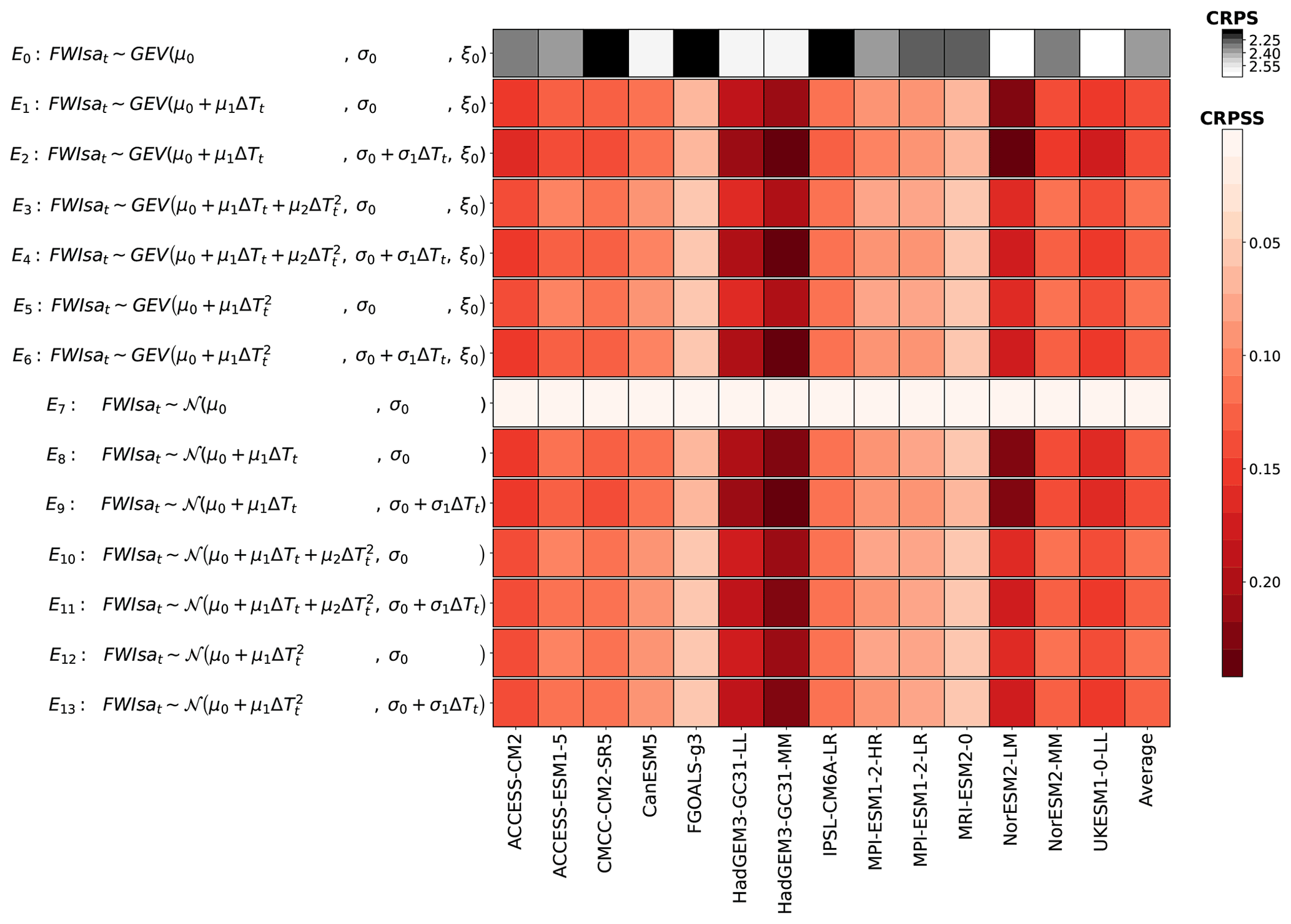
Figure 1Selection of the configuration for the seasonal average of the FWI (FWIsa). For each ESM, the CRPS and CRPSS are averaged over space, time, and scenarios. The darker the color of a cell, the better the configuration is at reproducing the distribution of the ESM. The upper row (white to black) corresponds to the CRPS of the configuration used as a benchmark. A higher CRPS (lighter color) indicates that the stationary distribution used as benchmark does not reproduce the distribution of the ESM well. The other rows (white to red) correspond to the CRPSS of the tested configurations relative to the benchmark. A higher CRPSS (darker color) indicates that the proposed configuration improves the reproduction of the distribution of the ESM.
A stationary GEV distribution is used as benchmark for all the other configurations. Comparing this benchmark E0 to a stationary normal distribution (E7) shows that the two of them are equivalent to the benchmark. We note that ESMs with higher CRPS tend to have higher CRPSS. For these ESMs, stationary distributions are worse at representing their potentially stronger climate signal, meaning that the improvement over a stationary distribution would be relatively high. We note that the two configurations with the best average CRPSS values are E2 and E9, which differ only in their distribution. Both have linear terms for location and scale. E2 performs slightly better than E9 because some points present skewed distributions that are better represented by a GEV distribution. Using quadratic evolutions tends to increase the performance of the fit in only a minority of grid points while decreasing the performance over the rest of the land area. For this reason, the results shown in Figs. 2 and 3 are performed using configuration E2. We point out that the local performances for this configuration are shown in the Appendix Sect. 6.4, along with those of the other variables emulated.
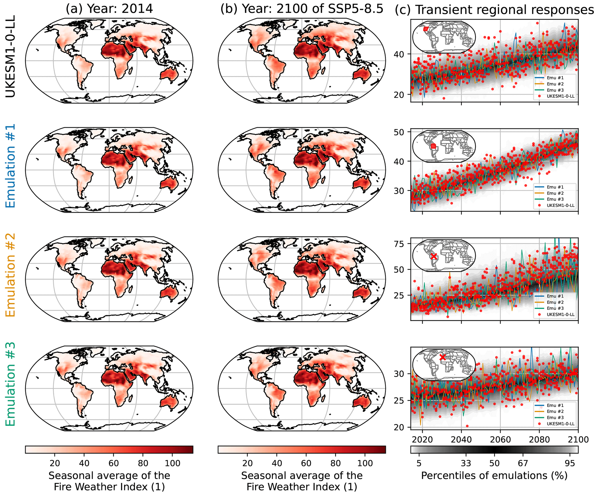
Figure 2Examples of results for the emulations of the seasonal average of the FWI (FWIsa) under UKESM1-0-LL. The left column (a) shows maps of FWIsa in 2014 according to UKESM1-0-LL in the first row, while the following three rows correspond to three emulations chosen randomly in the full set. The middle column (b) reproduces the same structure but in 2100 for SSP5-8.5. The third column (c) shows the time series of UKESM1-0-LL, the three emulations used for maps, and the full spread of the emulations (shaded area). The rows in (c) correspond from top to bottom to the western part of North America, the northern part of South America, a grid point in Amazonia close to Manaus, and a grid point in Portugal close to Lisbon.
In Fig. 2a and b we show examples of emulations illustrating the capacity of the emulator, here UKESM1-0-LL, shown in the top row. Be it in 2014 or in 2100, the three random emulations on the three other rows reproduce the spatial patterns of the ESM. There are some minor differences that are related to internal variability (ESM) and the stochastic representation thereof (emulator). Figure 2c illustrates the transient responses for FWIsa in the emulations and in the ESM over the course of SSP5-8.5. Note that each row of Fig. 2c is a chosen grid point or regional average. The red dots correspond to the realizations by UKESM1-0-LL for all ensemble members available, while the shaded black area represents the distribution of emulations. Over 2014–2100, the realizations by UKESM1-0-LL remain mostly within the range of the emulations, except for the third row, which corresponds to a grid point close to Manaus in Amazonia. Figures similar to Fig. 2 are provided in the Appendix Sect. 6.5 for low- and medium-warming scenarios.
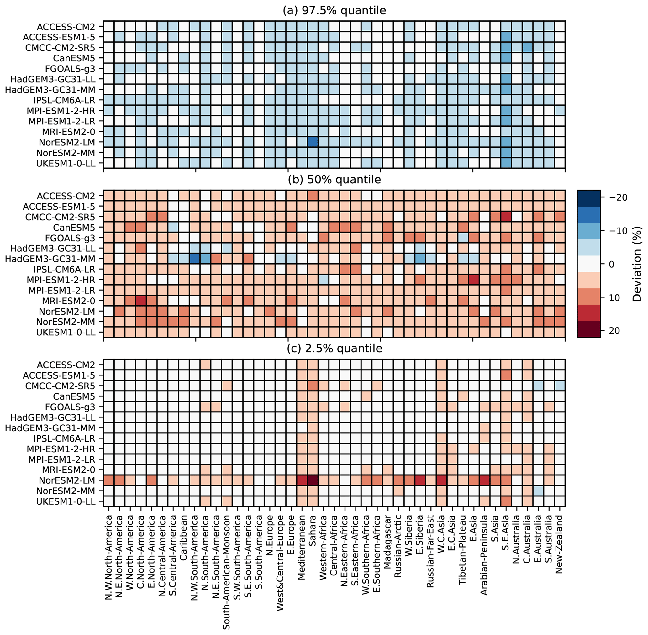
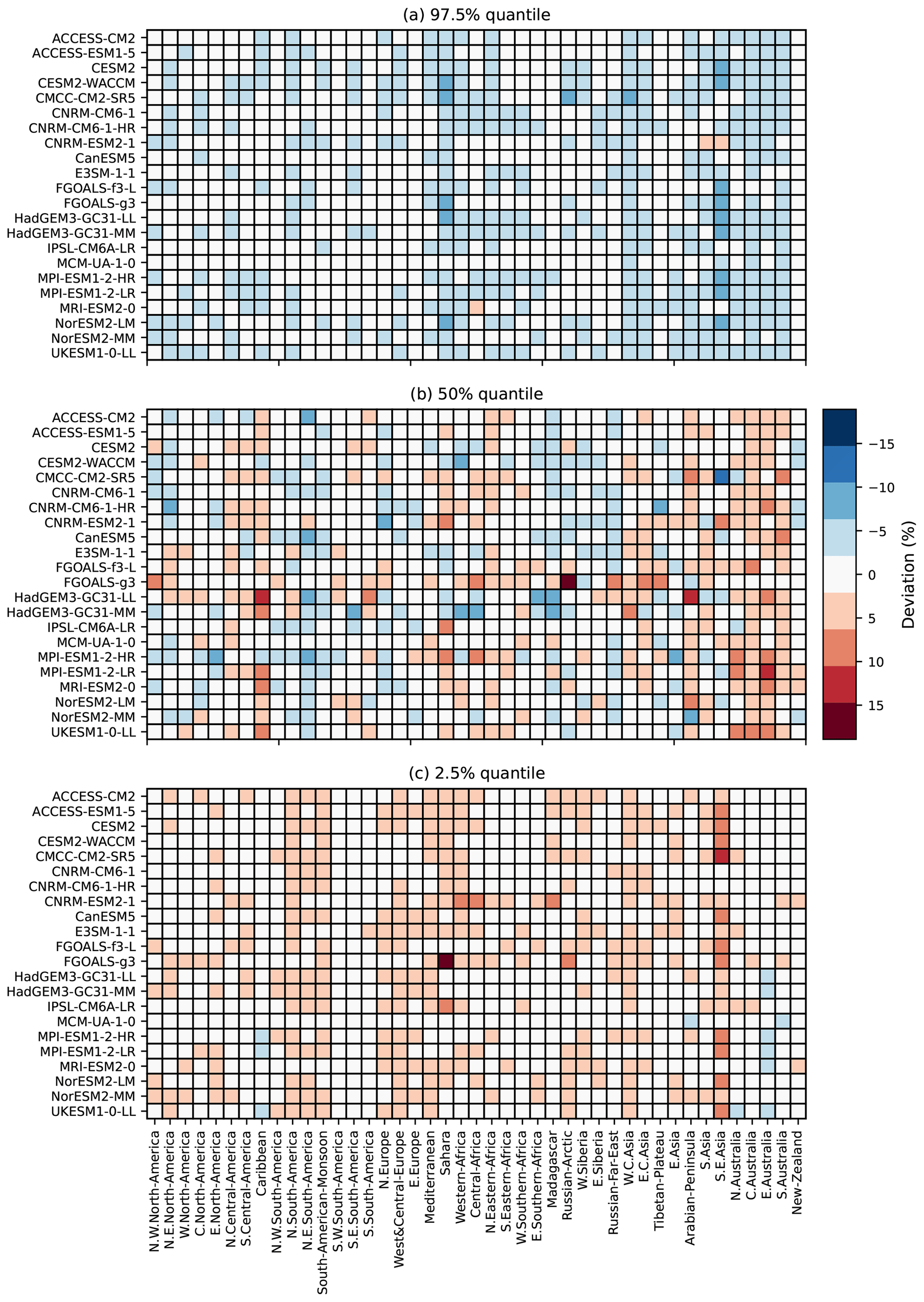
Figure 3 provide more details on the deviation of quantiles of MESMER-X for each ESM and land region (Iturbide et al., 2020), thereafter called ESM × regions. Overall, Fig. 3a shows that the quantiles at 97.5 % of the emulations are lower than those of the ESMs but higher for the quantiles at 2.5 % shown in Fig. 3c. This underdispersion is common for spatial emulators (Beusch et al., 2020a; Quilcaille et al., 2022), and regional aggregation contributes to this effect. For the quantile 97.5 %, the deviation of quantiles range from +1.5 % to −7.3 %, with an average of −1.5 %. In other words, the quantile 97.5 % of the emulations would actually instead be at 96 % on average when compared to the ESMs. For the median, the deviations range from −8.4 % to 13.3 %, with an average of −0.3 %. Finally, the deviations at the quantile 2.5 % range from −1.2 % to 16.0 %, with an average at 2.2 %. We note that the stronger deviations on the median occur when replicating NorESM2-LM. Because MESMER-X only aims at replicating the behavior of ESMs, it cannot be used to diagnose the reasons for this difference. First analyses might suggest that the response of FWIsa to ΔT is stronger than for other ESMs and that quadratic terms in the configurations may have a greater importance for this model.
In summary, the deviations of quantiles are less than 5 % in absolute value for at least 92 % of the ESM x regions. For the quantiles 97.5 %, 50 %, and 2.5 %, these proportions of ESM x regions below 5 % of deviation are 98 %, 93 %, and 92 %, respectively.
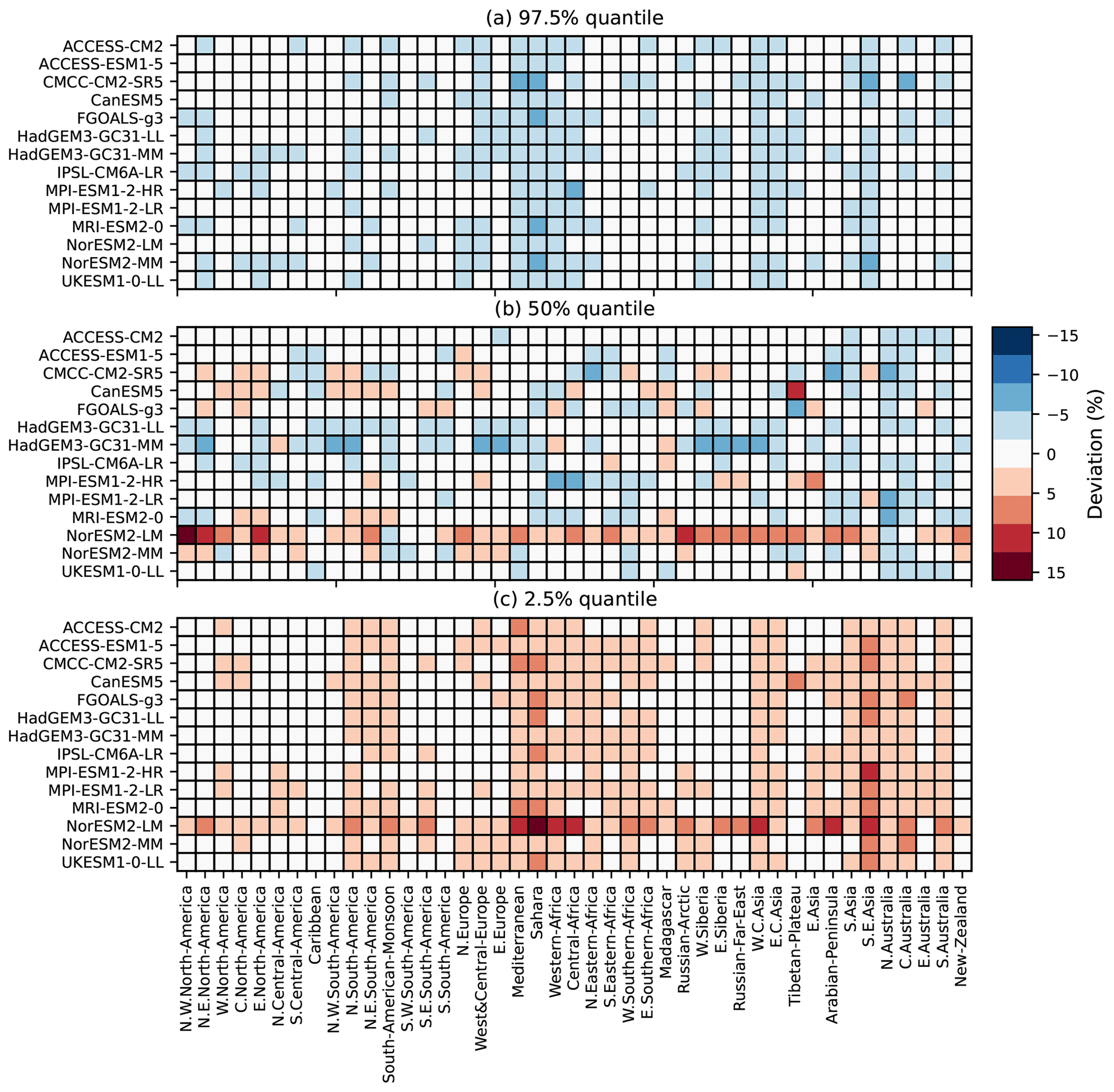
Figure 3Deviations of quantiles for the seasonal average of the FWI (FWIsa) at each ESM and each AR6 region. A positive deviation of quantiles (red) indicates that the quantile of emulations is higher than the one of the ESM, found by counting how often the ESM crosses the threshold set by the emulations. The deviation is calculated for all available scenarios. The upper panel (a) shows the deviations for the quantile 97.5 %, the middle panel (b) shows the deviations for the median, and the lower panel (c) shows the deviations for the 2.5 % quantile.
3.3 Emulation of the number of days with extreme fire weather
For emulating the number of days with extreme fire weather (FWIxd) we consider the Poisson distribution since it describes number of events occurring over a fixed period (Coles, 2001). Using this distribution implicitly assumes that the events are independent of each other, which is not exactly the case here. For instance, assuming that a day matches the criteria for extreme fire weather (Quilcaille et al., 2023) during the fire season, there are is a higher chance to have the next few days also matching this criterion compared to a period out of the fire season. Nevertheless, we choose this distribution because of its relative simplicity. Similarly to FWIsa, linear and quadratic terms are investigated given the physical basis and the observed responses to ΔT (Jain et al., 2022). The comparisons of the envisioned configurations are summarized in Fig. 4. Here, the parameters α introduced in Eq. (1) are the rate λ and a shift μ in the distribution. This modified form of the Poisson distribution has the same variance (λ) as the original Poisson distribution, but the mean is μ+λ instead of λ. This shift in the Poisson distribution allows for more flexibility in the training.
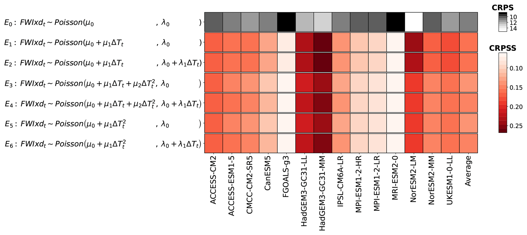
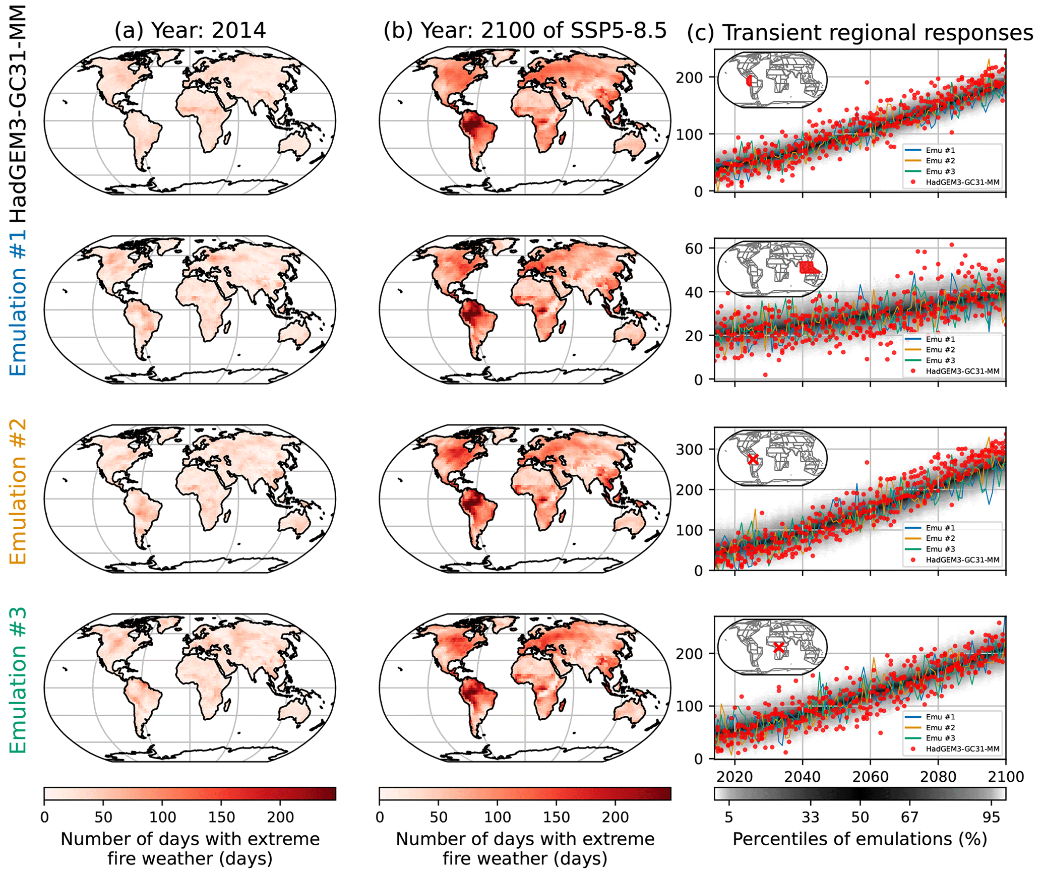
Figure 5Similar to Fig. 2 but for the number of days with extreme fire weather (FWIxd) under HadGEM3-GC31-MM. The rows correspond, from top to bottom, to the northwestern part of South America, Southeast Asia, a grid point in Amazonia encompassing the Jaú National Park, and a grid point in the Democratic Republic of the Congo encompassing the Salonga National Park.
A stationary Poisson distribution is used as benchmark, showing a range of performances in CRPS FWIxd (9 to 15) that is greater than the one obtained for FWIsa (2.1 to 2.6). Because the higher the CRPS is, the worse the distribution will be at representing the training sample, two results can be deduced. First, stationary GEV distributions are much better at reproducing FWIsa than stationary Poisson distributions are at reproducing FWIxd. This may be because FWIxd has stronger responses to climate change than FWIsa, meaning that stationary distributions (Poisson or GEV) cannot correctly reproduce these evolutions. This may also be because the shape of a Poisson distribution cannot reproduce the shape of the observed FWIxd as well as a GEV can for FWIsa. From Fig. 4 we observe that the best configuration is E1, which only shows a linear evolution of the location of the distribution. The configuration E2 had almost the same quality, albeit not as good for CMCC-CM2-SR5, MPI-ESM1-2-HR, and NorESM2-LM. Like FWIsa, few grid points, especially in South America, would benefit from a quadratic term. However, increasing the complexity of the functions for the parameters improved the fit only at a few grid points, while decreasing the performance in many other places. The configuration E1 has the best overall performance in spite of its simplicity; thus, we use this one for the results presented in Figs. 5 and 6.
Just like in Fig. 2, in Fig. 5 we show examples of outputs for the emulation of FWIxd. The spatial patterns are well respected overall, be it in 2014 or in 2100 (Fig. 5a, b). There are indeed some differences due to natural variability. For instance, in 2014 (Fig. 5a) HadGEM3-GC31-MM returns higher FWIxd to the south of the Sahel but lower values in South America. In 2100 (Fig. 5b), in the center of Africa and in Southeast Asia we see differences in these patterns, although the emulations are always relatively similar. Looking at the transient regional responses (Fig. 5c), the two regions and the two grid points represented show that HadGEM3-GC31-MM and the emulations have similar evolutions, with the distribution of the emulations correctly encompassing the dispersion of the ESM. We point out one exception in these time series in the third row. This grid point in Amazonia shows that the FWIxd of HadGEM3-GC31-MM increases faster than the emulations replicate. The same effect appears in the first row, albeit to a lesser extent. Some grid points in South America would benefit from a quadratic response to ΔT, although Fig. 4 shows that a linear response has better overall performances. Figures similar to Fig. 5 are provided in Appendix Sect. 6.6 for low- and medium-warming scenarios.
In Fig. 6 we show the regional performance of the emulator by assessing the deviations of its quantiles to the ESM. On average, the emulators are −2.8 % lower than ESMs for the 97.5 % quantile, 4.4 % higher for the median, and 1.41 % higher for the 2.5 % quantile. Overall, the emulators show lower performances in some regions, such as Southeast Asia, as shown in Fig. 5, or mimic some models such as NorESM2-LM. Explanations for the latter cannot be pinpointed to specific processes, as explained in Sect. 3.2. We observe that the median shows overall lower performance than the tails of the distribution.
To summarize the performances for FWIxd, the deviations of quantiles are less than 5 % in absolute value for 95 % of the ESM x regions at the 97.5 % quantile. At the 2.5 % quantile, the fraction of these ESM x regions below 5 % of deviation decreases to 92 %. However, at the median only 54 % of the ESM x regions are below 5 % of deviation. A potential explanation may be the temporal dependence of the events not respecting one of the conditions for the use of a Poisson distribution. As detailed at the beginning of this section, this work using a Poisson distribution is a first attempt with discrete distributions. Using other distributions that would not assume independent events may improve these results but would require a higher degree of complexity.
4.1 Data for the annual indicators of soil moisture
We base the annual indicators for soil moisture on the total soil moisture content (CMIP6 variable mrso). Ideally, soil moisture in the root zone would be more relevant to investigate droughts. Thus, soil moisture in the soil layer (CMIP6 variable mrsos or mrsol) would have been more adapted (Qiao et al., 2022). Similarly, the total soil moisture content includes all water phases and thus frozen soil moisture as well. We deem that the total soil moisture content remains relevant for droughts in regions without high frozen soil moisture, i.e., not at higher latitudes or in mountainous regions like the Himalaya. Nevertheless, a majority of ESMs only provide the total soil moisture content, thus choosing this variable ensures that the capacity of the emulator can be evaluated on more models and ensemble members.
Before computation of the annual indicators, the total soil moisture content of all available CMIP6 runs is regridded onto a common longitude–latitude grid using second-order conservative remapping (Jones, 1999; Brunner et al., 2020).
Two annual indicators are deduced from the total soil moisture content. By averaging this variable over the year, we obtain the annual average of soil moisture (SM). In addition, we calculate the average over each month and deduce their minimum, thus obtaining the annual minimum of the monthly average soil moisture (SMmm). These two annual indicators are both relevant to assess the evolutions of droughts (Cook et al., 2020). The annual average SM provides an indicator for the whole year, while the annual minimum SMmm informs us about the worst period of the year.
4.2 Emulation of the annual average of soil moisture
As for the fire weather, the first step for emulation is to choose a proper distribution. As an annual average, SM may be represented by a normal distribution according to the central limit theorem. The second step is to propose evolutions for the parameters. The impact of global temperature on the local total soil moisture content is not as straightforward as for the two former cases. Many processes affect this variable, through evapotranspiration, precipitation, or runoff (Cook et al., 2020). Some regions show a decreasing trend in the soil moisture, others an increase (van den Hurk et al., 2016; Qiao et al., 2022). A first choice could be to propose a linear evolution on the mean (Greve et al., 2018). However, going through local responses of SM to ΔT shows that they may often be nonlinear, e.g., following a sigmoid response. Such responses are characteristic of an evolution between two regimes, as illustrated in Fig. 7.
Another feature of these local responses is their lagged effects. The response under SSP1-2.6 (blue points) decreases faster with ΔT than SSP2-4.5 (dark green points). The same effect happens with SSP3-7.0 (brown points) and SSP5-8.5 (orange points). The faster the warming increases, the slower the slope is in the response of SM to ΔT. A potential explanation would be that different timescales are at play in the response of SM to ΔT. In high-warming scenarios, the ΔT increases relatively quickly in the response of SM to the change in ΔT and does not let the SM stabilize. However, in SSP1-2.6 the ΔT stabilizes, allowing the SM to stabilize as well. To a broader extent, this effect is related to the response of the whole water cycle, with rapid adjustments and slow feedback responses both in precipitation and evapotranspiration (Allan et al., 2020). Different methods may be used to represent the effect of different timescales, such as lagged variables or impulse response functions. Here, as a first attempt to reproduce this effect, in this configuration we will test a lagged variable using the ΔT at the former year. This lagged variable is obtained by shifting the ΔT of the ESM by 1 year. From a modeling perspective, having both ΔTt and ΔTt−1 is equivalent to having the value at year t and its first derivative.
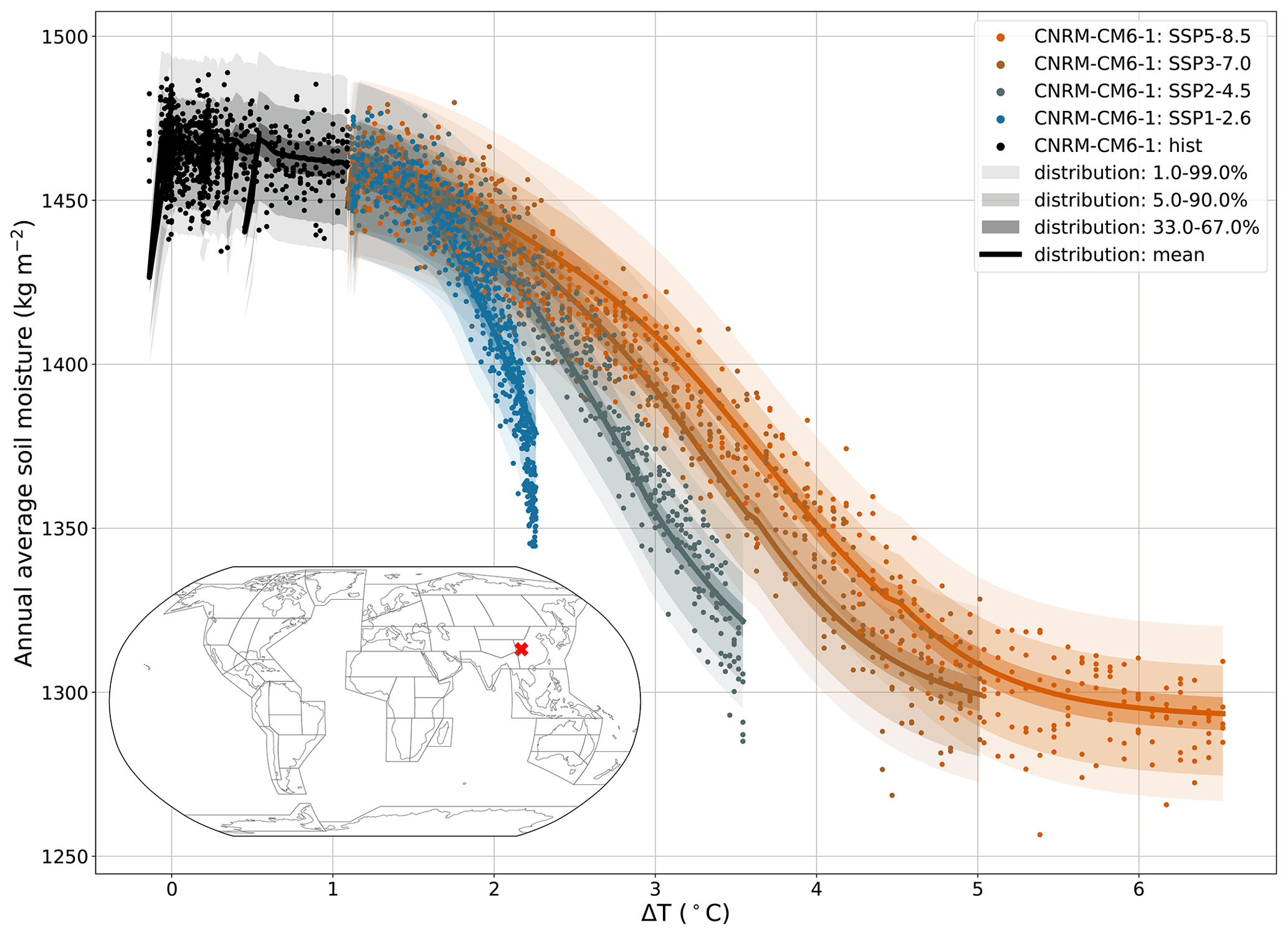
Figure 7Example of local response of the annual average soil moisture (SM) to ΔT under CNRM-CM6-1. The grid point is in Sichuan, in the vicinity of Chengdu, i.e., the same one shown in the fourth row of Fig. 9c. The distribution shown follows the configuration E4 described in Eq. (12).
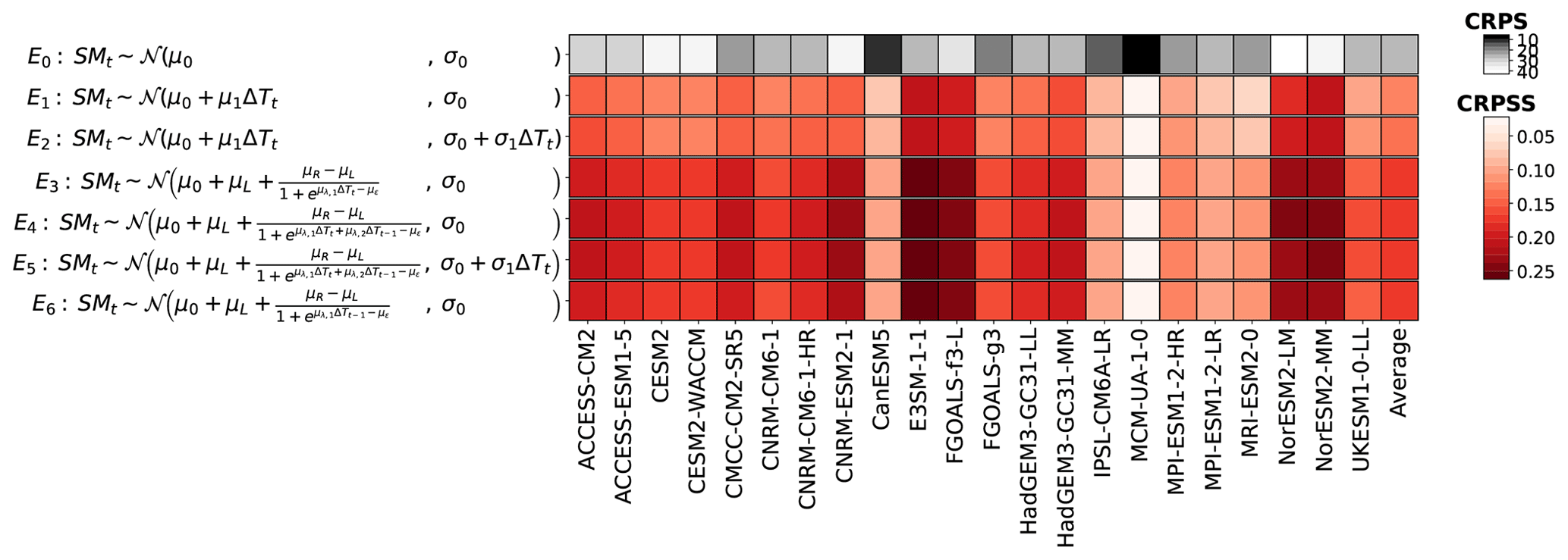
Figure 8 shows the results for all the tested configurations, with the coefficients μ and σ corresponding to the location and the scale of the normal distribution, respectively. For all ESMs except ACCESS-ESM1-5 and CNRM-ESM2-1, the best performances according to the CRPSS are met with E4. For these two other ESMs, the better configuration E5 differs only from the linear response on the standard deviation of the distribution. We note that introducing a logistic response on the mean (E3) improves the performances in a large majority of the grid points more than a linear effect (E1). Introducing the lagged effect has an effect that is not as clear (E4) because the CRPSS is averaged over time and different scenarios. Given these results, we choose to use the configuration with the best performance for most ESMs. The results presented in Figs. 9 and 10 will then use the configuration E4.
In Fig. 9, we illustrate the emulations of SM for CNRM-CM6-1. Just like for FWIsa (Fig. 2) and FWIxd (Fig. 5), the spatial patterns are correctly reproduced. Note that the mean climate signal is dominant, and thus the effects of internal variability are hardly visible. The time series in Fig. 9c show, however, that the natural variability is in general well reproduced over the course of SSP5-8.5. In the region of western and central Europe, the ESM seems to often be below the 5 % quantile of the emulations, especially around 2050. In the region in the western part of of southern Africa, the spread of the distribution is relatively large but represents the spread of the ESM in this region relatively well. We point out that the six ensemble members shown in Fig. 9 combined as a large regional spread show many points relatively far from the 90 % range of the emulations, but the repartition of the realizations by CNRM-CM6-1 in this region is still well respected. Figure 9c shows, however, that some aspects of the dynamics are not entirely captured by the emulator, such as the short increase over 2040–2050 in Brazil. It may indicate that choosing the ΔT over the former year is not good enough to represent lagged effects or that there are additional processes that cannot be represented as such by MESMER-X. Figures similar to Fig. 9 are provided in the Appendix Sect. 6.7 for low- and medium-warming scenarios.
In Fig. 10, we show the deviations of the regional quantiles of the emulations in each ESM x region. Just like with FWIsa (Fig. 3) and FWIxd (Fig. 6), the emulations are overall under-dispersive. The 97.5 % quantile (Fig. 10) shows that the emulations have their quantiles −1.9 % on average lower than their ESM counterparts, up to −10.3 %. There, the lower performances of MESMER-X occur in Sahara and in South-East Asia. Figure 10b shows that the median of emulations is on average 0.4 % higher than the ESMs, these deviations ranging from 18.9 % to −12.7 %. We note lower performances in regions of Australia and in the Caribbean. Finally, the deviations of the 2.5 % quantile show that the emulations are on average 1.5 % higher than the ESMs, up to 15.7 % of deviations. The emulator for FGOALS-g3 exhibits lower performances than for other ESMs, although the reason for this remains unclear.
As a summary of the performances of the emulations of SM, the deviations are limited to 5 % in 96 % of the ESM x regions at the 97.5 % quantile, 88 % at the median, and 97 % at the 2.5 % quantile.
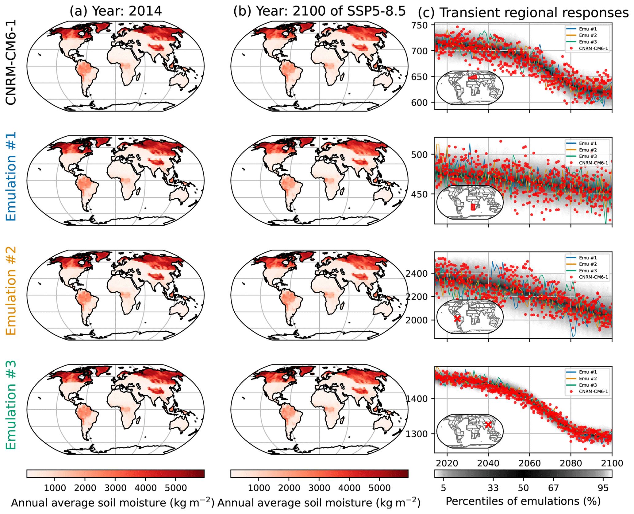
Figure 9Similar to Fig. 2 but for the annual average soil moisture (SM) under CNRM-CM6-1. The rows correspond from top to bottom to western and central Europe, the western part of southern Africa, a grid point in the west of Brazil in the state of Acre, and a grid point in Sichuan, China, close to Chengdu.
4.3 Emulation of the annual minimum of the monthly average of soil moisture
Emulating the annual minimum of the monthly average soil moisture is analogous to the emulation of annual average soil moisture. As an average over a month, SMmm may be represented using a normal distribution, although the minimum values over the months may be represented by a GEV distribution. However, sampling a block maxima over 12 values (each month) is too small to converge towards a GEV distribution. Thus, a normal distribution is used. Checking the local evolutions of the sample leads to similar observations to those observed for the annual average of the soil moisture illustrated in Fig. 7. Thus, the same configurations are used for SMmm as for SM.
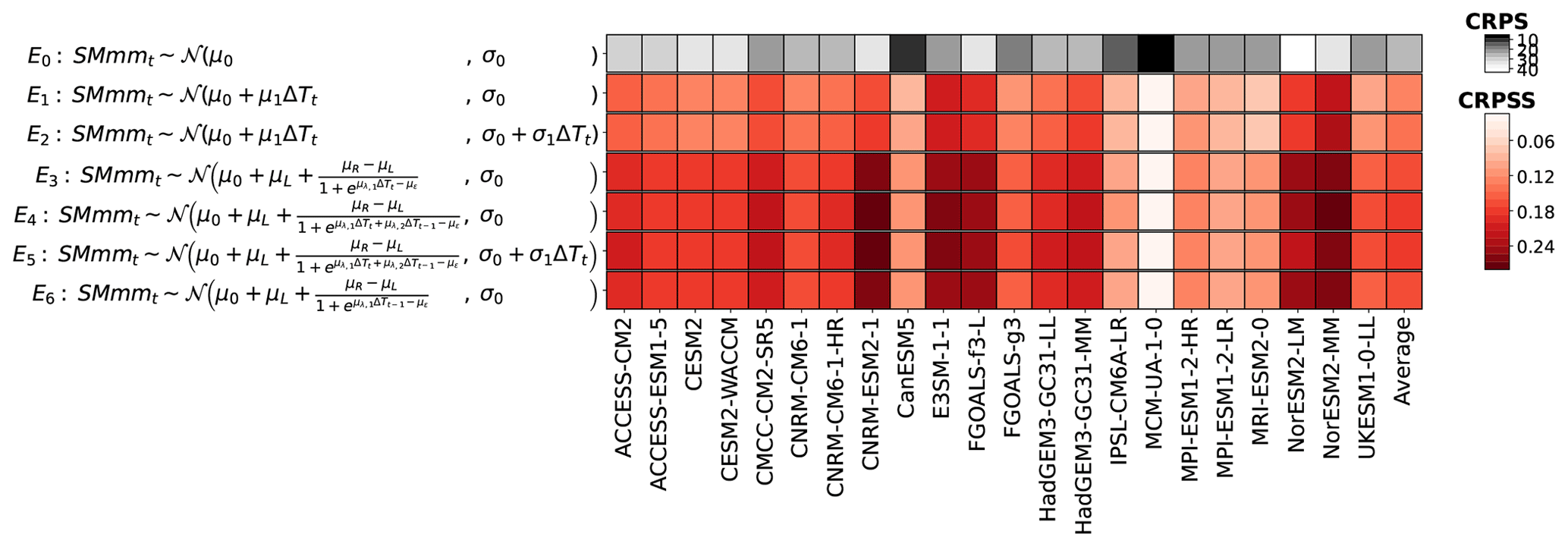
Figure 11Similar to Fig. 1 but for the annual minimum of the monthly average of soil moisture (SMmm).
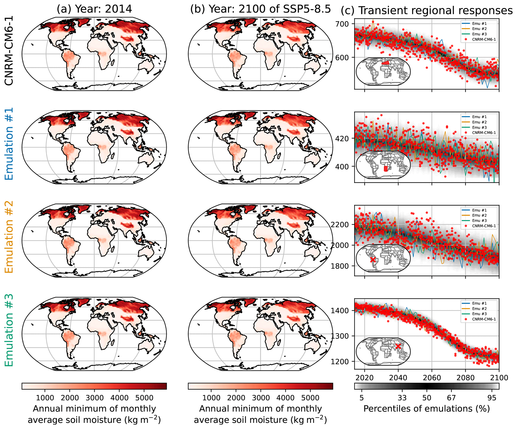
Figure 12Similar to Fig. 2 but for the annual minimum of the monthly average of soil moisture (SMmm) under CNRM-CM6-1. The rows correspond, from top to bottom, to western and central Europe, the western part of southern Africa, a grid point in the west of Brazil in the state of Acre, and a grid point in Sichuan, China, close to Chengdu.
In Fig. 11 we summarize the performances for the emulations of SMmm over the different configurations, with the coefficients μ and σ corresponding to the location and the scale of the normal distribution, respectively. The configuration with the best performance is E4, with the mean as a logistic function of ΔT at the year and the former year, while the standard deviation remains constant.
Note that both SM and SMmm have the same best configuration. Both annual indicators are averages and SMmm has SM as its upper limit, which may explain this result. We also note that ACCESS-CM2 shows better performance with a linear evolution of the standard deviation, although the opposite occurs with NorESM2-LM. Without logistic evolution, we note lower performances for high-warming scenarios because linear fits fail at reproducing the nonlinear evolutions at high ΔT. Without ΔT at the former year, the performances of the emulations are reduced for low-warming scenarios because the water cycle get more time to stabilize to the current regime.
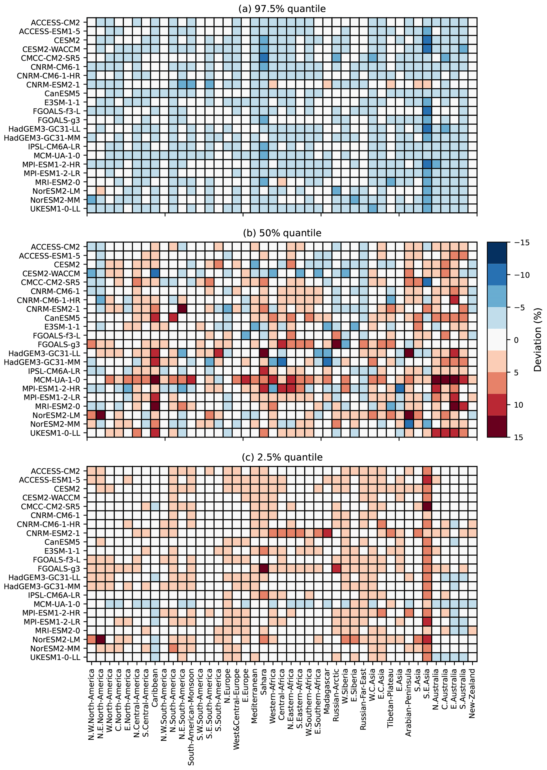
Figure 13Similar to Fig. 3 but for the annual minimum of the monthly average of soil moisture (SMmm).
The results for the emulations of SMmm under this configuration are illustrated in Fig. 12. The spatial patterns of the ESM shown here on the top row, CNRM-CM6-1, are correctly reproduced by the emulations on the three following rows. The right column shows that the regional responses are correctly reproduced, with a majority of the ESM points being within the range of the emulations. Their dispersions seem to respect the distribution of the emulation, as will be confirmed with the regional performances in Fig. 13. Just like SM, the realizations by CNRM-CM6-1 in the grid point in Brazil in the third row of Fig. 12c show a decrease in SMmm over 2020–2050, then an increase over 2050–2060, and then a decrease over 2060–2100. In the meantime, the emulations fail to reproduce these evolutions, decreasing at a slower pace over 2020–2050 and not increasing over 2050–2060. The processes explaining such evolutions are not reproduced by the emulator, and more research would be needed to integrate them. Figures similar to Fig. 12 are provided in the Appendix Sect. 6.8 for low- and medium-warming scenarios.
The performance of the emulations for the retained configuration for SMmm are shown in Fig. 13. The deviations of the quantiles of the emulations in the ESMs are summarized for each ESM and AR6 region, respectively, at the 97.5 %, 50 %, and 2.5 % quantiles. The emulators are again overall under-dispersive. On average, the fraction of points above the 97.5 % quantile of emulations indicates that this quantile of the emulations is too low by −2.0 %. At the median, the emulations are +1.1 % too high. At the 2.5 % quantile, the emulations are +1.4 % too high. The fraction of ESM x regions with a deviation of the quantiles limited to 5 % is limited to 96 % for both 97.5 % and 2.5 % quantiles and 85 % for the median. Overall, the distributions are relatively well reproduced, although some regions show lower performances. Here again, the emulator performs lower in Southeast Asia than in the other regions. As explained in other sections, this may be an effect of fewer land grid points affecting the reproduction of spatial correlations. On the median, the emulator of MCM-UA-1 has a lower performance than for the other ESMs. The emulator of NorESM2-LM has a lower performance than for the two other shown quantiles. These results cannot be used directly to diagnose different effects in the ESMs. Instead, further research will be needed to understand and integrate these effects in the modeling framework of MESMER-X.
The emulator MESMER-X, an extension of the MESMER emulator (Beusch et al., 2020a, 2022b), which is focused on the emulation of impact-relevant variables, including extremes, was introduced and showcased for TXx (Quilcaille et al., 2022), suggesting a potential for extension to other climate variables. Here, we have confirmed this potential with a range of yearly indicators of the fire weather index and soil moisture. We illustrated that several distributions may be used in this framework, such as the GEV for TXx and FWIsa, the normal distribution for SM and SMmm, and finally the Poisson distribution for FWIxd. It clearly shows how the MESMER-X framework can be easily adapted to sample from additional probability distribution, thereby facilitating its adaptation to further climate variables. Moreover, the nonlinear response of soil moisture to global mean temperature required a more sophisticated parameterization, including a logistic response and the consideration of time-lagged predictor variables. This latter extension highlights that the MESMER-X setup can be easily adapted to also account for a nonlinear climate response in the considered variable.
We have shown good performances for these emulators, typically with deviation of quantiles limited to 5 % in about 90 % of the ESM x AR6 regions, with variations in the indicators and quantiles. We have pointed out some limitations. The main one was observed with FWIxd, with lower performances on the median of emulations. In this case, the Poisson distribution may not be adequate, and more flexibility in the moments of the distribution may be necessary, e.g., to allow fat tails. Another limitation is that there are regions that would benefit from local responses with different parameterizations, e.g., with fire indicators in South America. Such effects have not been accounted for here to preserve simplicity in the modeling. Making parameterizations dependent on the grid point would be a solution but was not implemented for this article. Finally, some local aspects of the dynamics are not captured by the emulations, e.g., with soil moisture indicators in Amazonia. Using time-lagged predictors may not be good enough locally, and there may even be processes that cannot be entirely captured in this framework.
Given these results, the further expanded MESMER-X emulator is capable of emulating several annual impact-related variables, including climate extremes and a drought-related water cycle variable, with satisfactory performance. It can emulate variables distributed over GEV, normal, and Poisson distributions. Linear, quadratic, and logistic evolutions of the parameters have been shown here. An example of a lagged effect is shown here. This method is very flexible, relatively simple, and yet has good performance. We have identified limitations but also proposed potential solutions.
The expanded MESMER-X is thus a tool now capable of exploring impact-related variables, including climate extremes and a drought-related water cycle variable, and may be used to provide information to assess climate impacts under a range of emissions scenarios, including the upcoming scenarios to be developed in preparation for the Seventh Assessment Report of the IPCC. As such, the MESMER-X emulator is complementary to the ESMs: it relies on ESMs for training but is fast enough for coupling with other models in need of climate information. Finally, ESMs may carry some biases (Kim et al., 2020) even for climate extremes (Schewe et al., 2019). Tools such as MESMER-X may foster the integration of observation constraints to correct these biases.
A1 Application of a probability integral transform to discrete distributions
The probability integral transform (PIT) introduced in Eq. (2) of this paper transforms values from a known distribution to another distribution, here a normal distribution of mean 0 and standard deviation 1, thus “Gaussianizing” the sample. We illustrate here how the PIT applies to discrete distributions. For the sake of clarity, these explanations are not based solely on statistical data instead of climate data.
Here we consider a GEV distribution and a Poisson distribution. To facilitate the comparison, the parameters are picked so that their cumulative distribution functions (CDFs) would be relatively similar. In Fig. A1 we show their respective CDFs and how the PIT would apply to two values.
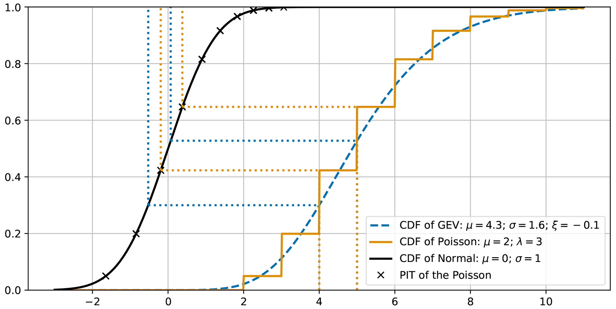
Figure A1Illustration of a probability integral transform applied to continuous and discrete distributions.
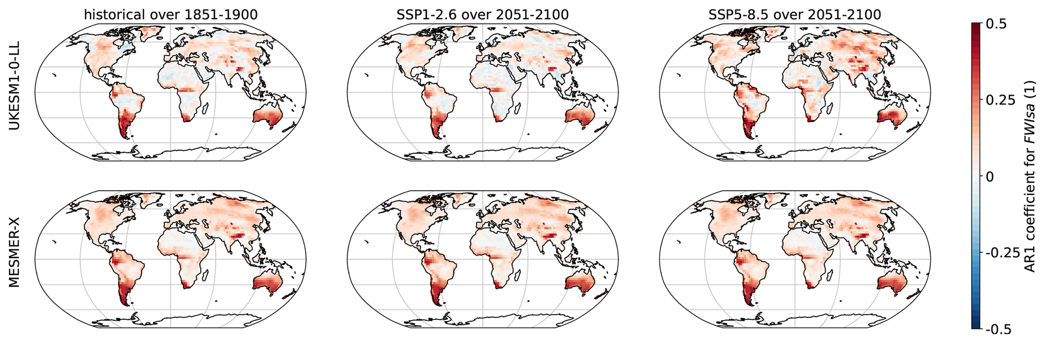
Figure A2First-order coefficient of a temporal auto-regressive process for FWIsa with UKESM1-0-LL and MESMER-X using the configuration presented in Eq. (10).
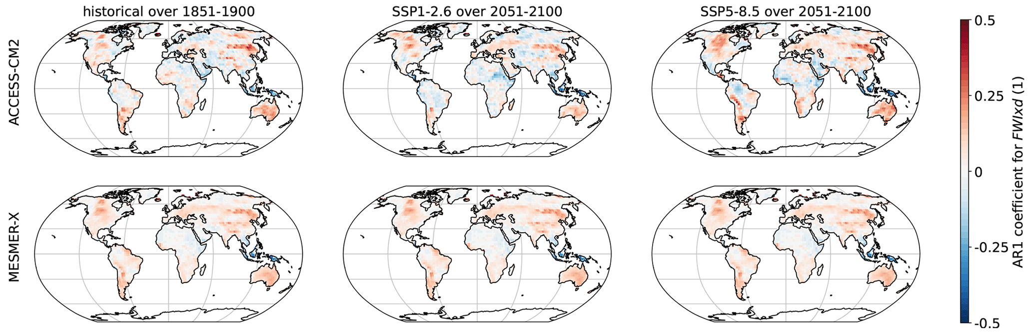
Figure A3First-order coefficient of a temporal auto-regressive process for FWIxd with ACCESS-CM2 and MESMER-X using the configuration presented in Eq. (11).
We note that events with a value of 4 would have higher transformed values under a Poisson distribution than under a GEV distribution. This observation may raise issues regarding the use of a PIT for a discrete distribution. However, a value of 4 is representative of the values in the interval [3.5; 4.5[. Thus, over [3.5; 4[, the transformed values over a Poisson distribution would be below those of a GEV, while over [4; 4.5[, they would be higher than those of a GEV. According to this effect, applying a PIT to a discrete distribution would lead to partially compensating errors.
Intervals from the discrete distribution are represented by a single value, thus a single value in the “Gaussianized” space. However, the realizations from the auto-regressive process with spatially correlated innovations are back-transformed using another PIT, as described in Eq. (7). These realizations are continuous, leaving only the values taken by a Poisson distribution after PIT. As such, the same effect occurs, albeit the other way round: intervals of values in the realizations are transformed into single values.
As a result, applying a PIT to a discrete distribution appears to have the intended effect. This is due to the matching of intervals of values to single values, which led to partially compensating effects. Furthermore, this effect occurs another time during the back transformation. We acknowledge the extent of the compensations of these effects, will investigate further in this direction, and welcome other contributions.
A2 Representation of the interannual variability for each variable
An important aspect of the impacts of climate change is their potential persistency. Hazardous climate conditions impact the Earth system and our societies, but such conditions maintained over several years may result in even higher impacts. For instance, droughts lasting several years would have stronger impacts in terms of food security than the impacts of non-adjacent droughts.
As such, representing the interannual variability matters when emulating variables related to climate impacts or the water cycle. In MESMER-X, it is modeled using an auto-regressive process of the first order, as shown in Eq. (3). It is applied on the climate variable after the probability integral transform of Eq. (2) to ensure the “Gaussianized” distribution required by the auto-regressive process. However, the training of this process is performed over the whole training sample, and the interannual variability of the ESM may change over time, for instance due to changes in large-scale oscillations.
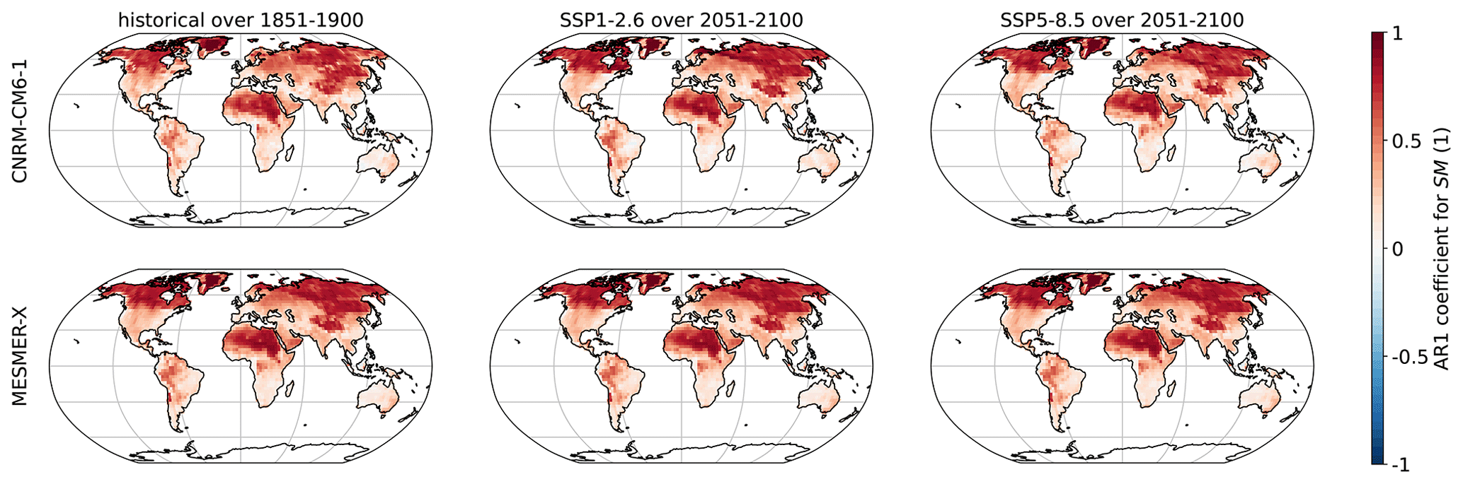
Figure A4First-order coefficient of a temporal auto-regressive process for SM with CNRM-CM6-1 and MESMER-X using the configuration presented in Eq. (12).
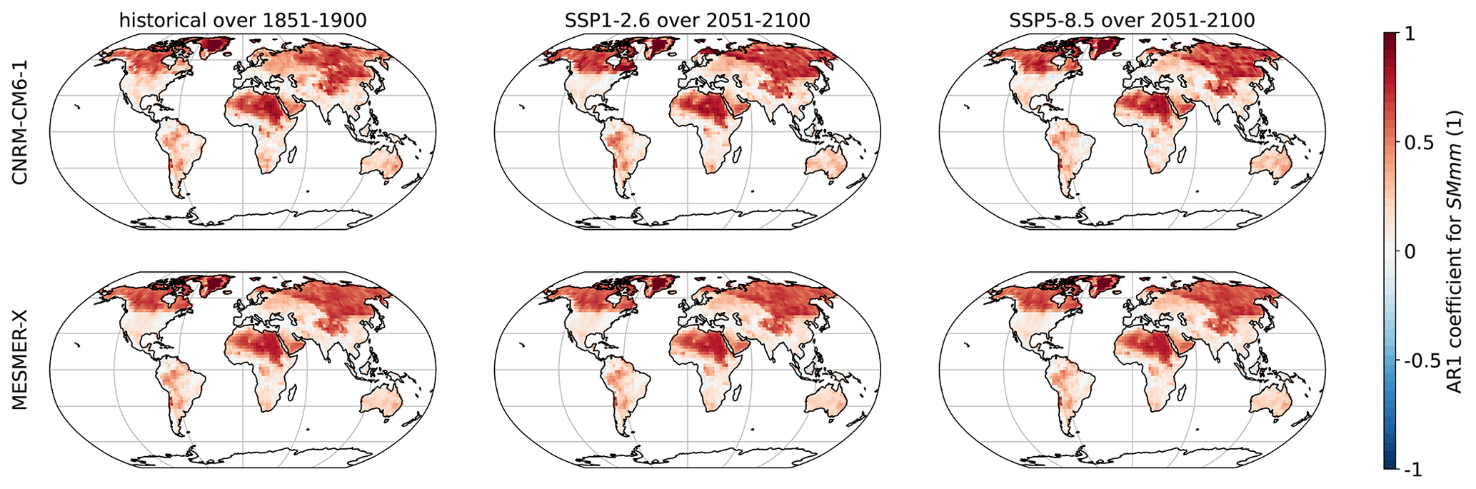
Figure A5First-order coefficient of a temporal auto-regressive process for SMmm with CNRM-CM6-1 and MESMER-X using the configuration presented in Eq. (13).
Here, we evaluate the local evolutions of the interannual variability in the trained ESMs and its representation by MESMER-X. For each climate variable emulated in this paper, we use the ESM used for illustration of its emulator in time series and maps. We choose three periods, the preindustrial (1851–1900), the end of a low-warming scenario SSP1-2.6 (2051–2100) and the end of a high-warming scenario SSP5-8.5 (2051-2100). In each case, we apply the probability integral transform as shown in Eq. (2) as a form of detrending and so that the new sample follows a standard normal distribution. In each grid point, we calculate an auto-regressive process of the first order and average its coefficient over available members. For the emulator, we verify that these calculations effectively lead to the parameters γs,1 of Eq. (3) because of the spatially correlated innovations over the realizations. All of these results are shown in Figs. A15 to A18.
These figures show that all the variables presented in this article are mostly positively correlated. In addition, SM and SMmm have higher correlations than FWIsa and FWIxd. This is due to inertia in the water cycle with a relatively long recovery time from droughts. The evolutions of these correlations in the ESM are relatively slow, mostly in Québec, Greenland, and Murmansk. Its MESMER-X counterpart is the average in time of these correlations, thus reproducing the interannual variability of the ESM well.
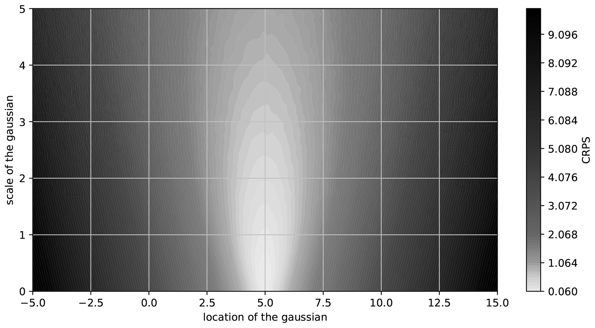
Figure A6CRPS obtained with an observed value of 5 and Gaussian distributions sampled over 10 000 members over different values of its parameters.
A3 Interpretability of the CRPS
All CRPS scores in this paper have been calculated thanks to the Python package properscoring available at https://pypi.org/project/properscoring/ (last access: 7 December 2023). More specifically, they have been created with its function calculating crps_ensemble. Below is an illustration of the CRPS obtained using this function.
For interpretability of the CRPS, one may consider the expression for an observation X and the normal distribution with f and F, its probability density and cumulative distribution functions, respectively, derived from Eq. (8.55), p. 353 of Wilks (2011):
Similar equations may be obtained for a GEV from Eq. (9) of Friederichs and Thorarinsdottir (2012) or other distributions (http://cran.nexr.com/web/packages/scoringRules/vignettes/crpsformulas.html, last access: 7 December 2023).
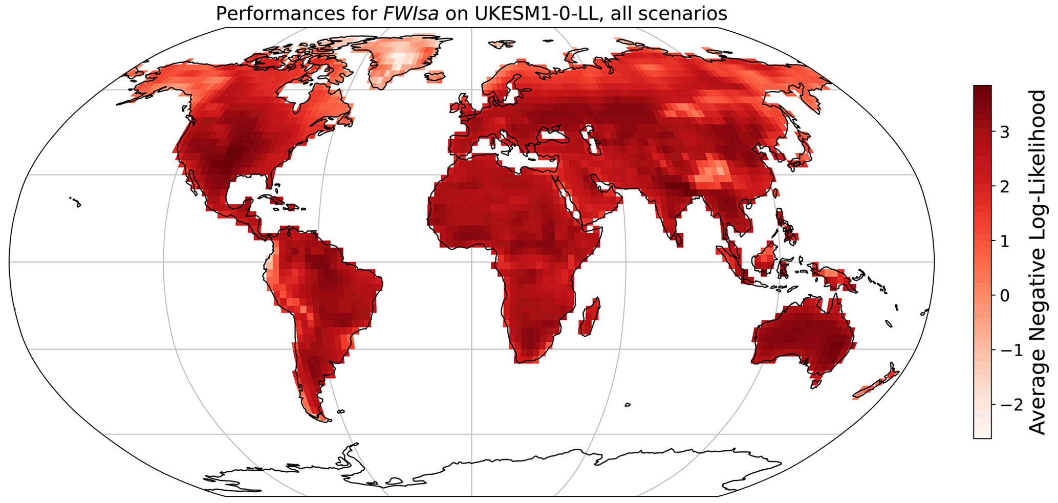
Figure A7Negative log likelihood obtained during training of MESMER-X on FWIsa using the configuration presented in Eq. (10) and for the ESM used in Fig. 2.
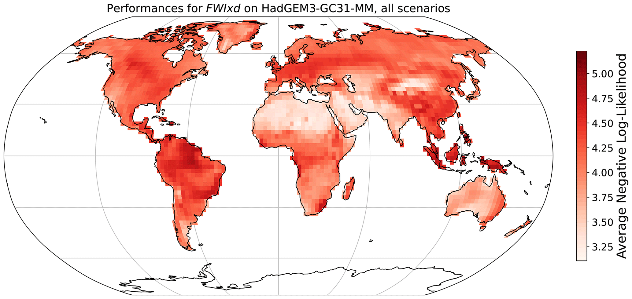
Figure A8Negative log likelihood obtained during training of MESMER-X on FWIxd using the configuration presented in Eq. (11) and for the ESM used in Fig. 5.
A4 Performances of the emulators for each variable
The grid-cell-level parameters of MESMER-X are trained by minimizing the negative log likelihood of the training sample given a prescribed configuration for each grid cell independently. We show here the averaged negative log likelihood at the grid cell level for the retained configuration and with the ESM used to illustrate the performance of MESMER-X. The value is averaged to account for the number of time steps used during training and to facilitate the comparisons.
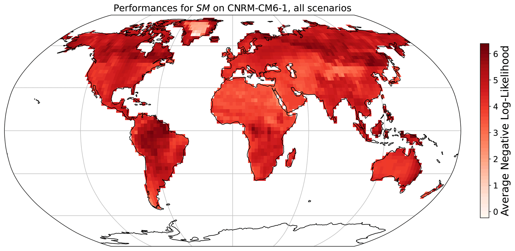
Figure A9Negative log likelihood obtained during training of MESMER-X on SM using the configuration presented in Eq. (12) and for the ESM used in Fig. 9.
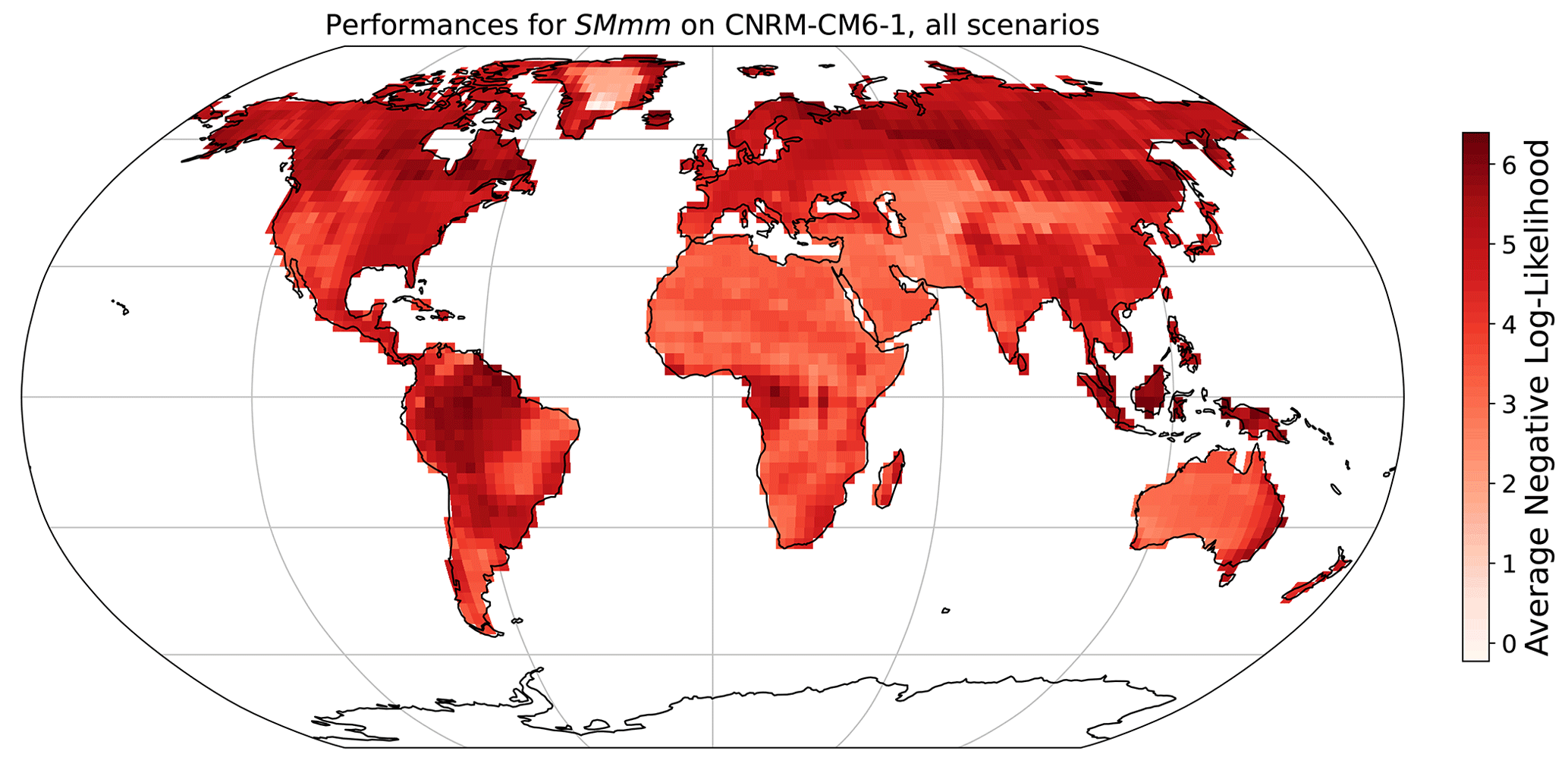
Figure A10Negative log likelihood obtained during training of MESMER-X on SMmm using the configuration presented in Eq. (13) and for the ESM used in Fig. 12.
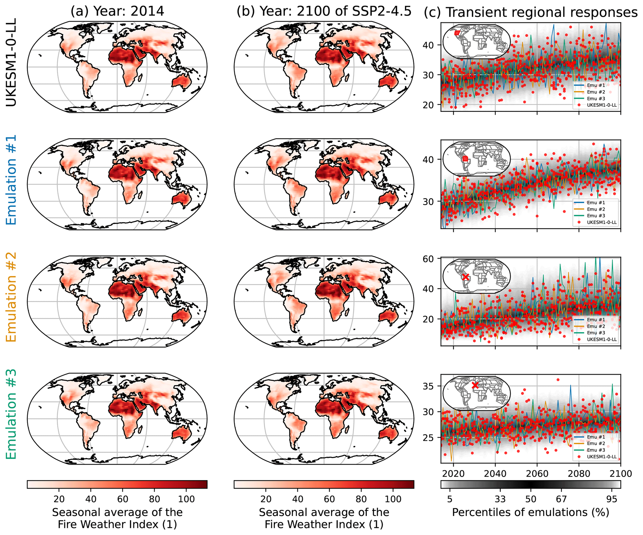
Figure A11Similar to Fig. 2 but with the medium-warming scenario SSP2-4.5.
A5 Emulations of the seasonal average of the Fire Weather Index over low- and medium-warming scenarios
In Sect. 3.2, we emulate the seasonal average of the Fire Weather Index (FWIsa), that we illustrate in Fig. 2 with the high warming scenario SSP5-8.5. While this scenario allows us to explore a large range of warming for the model, it does not show evolutions over more advisable warming ranges, nor does it show potential stabilization effects over low-warming scenarios. Here, we produce the equivalent of Fig. 2 for SSP1-2.6 and SSP2-4.5.
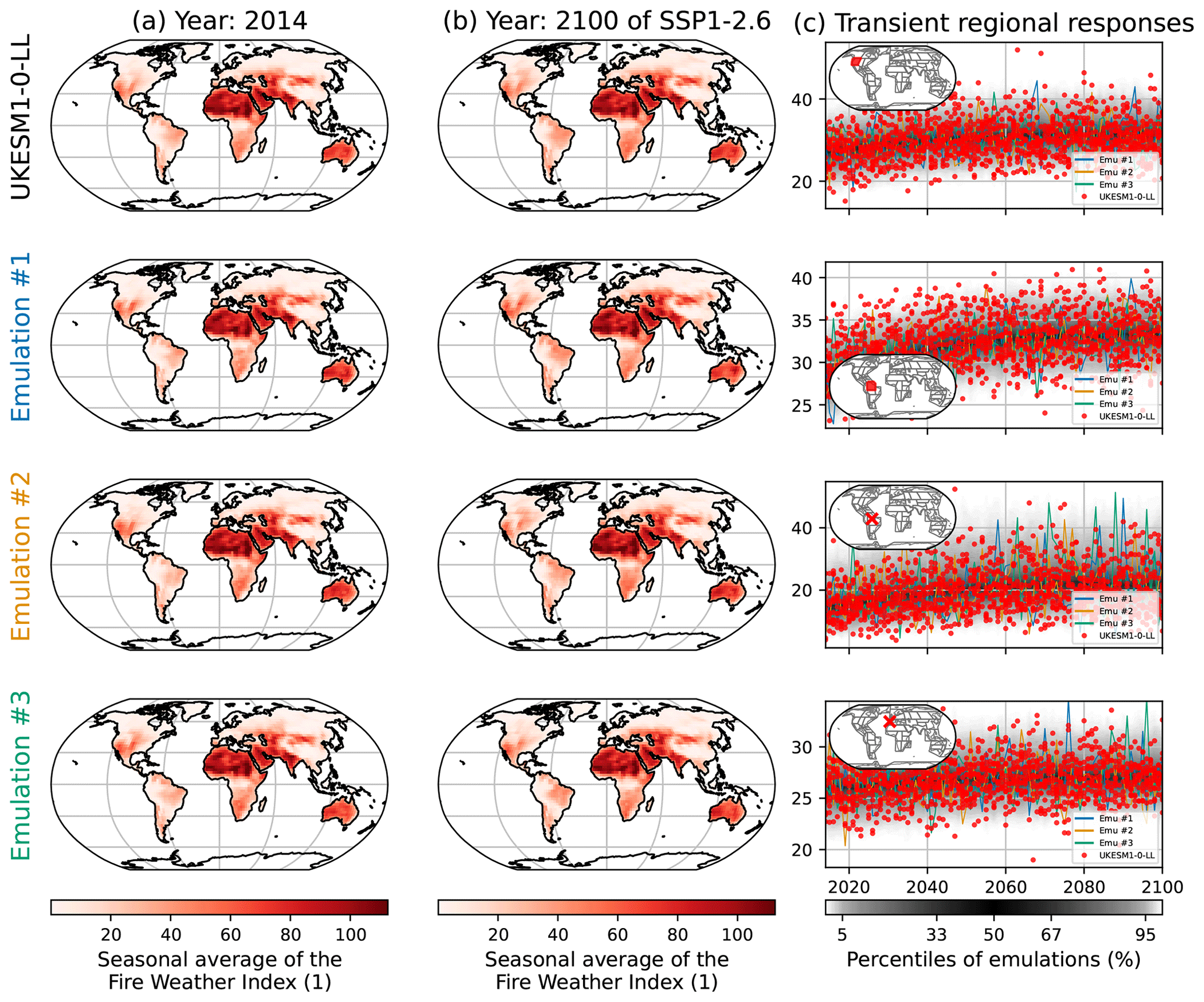
Figure A12Similar to Fig. 2 but with the low-warming scenario SSP1-2.6.
A6 Emulations of the number of days with extreme fire weather over low- and medium-warming scenarios
As was done in Sect. 6.3 for the seasonal average of the Fire Weather Index, we extend Sect. 3.3, where we emulated the number of days with extreme fire weather (FWIxd) and illustrated the result in Fig. 5 using the high-warming scenario SSP5-8.5. Again, while this scenario allows us to explore a large range of warming for the model, it does not show evolutions over more advisable warming ranges, nor does it show potential stabilization effects over low-warming scenarios. Here, we produce the equivalent of Fig. 5 for SSP1-2.6 and SSP2-4.5. We highlight that the SSP2-4.5 was not provided by the ESM HadGEM3-GC31-MM. In addition, its counterpart HadGEM3-GC31-LL provided only one member for SSP1-2.6. For the sake of visualization, we opt to show the results with ACCESS-CM2, which provided five members for both SSP1-2.6 and SSP2-4.5.
A7 Emulations of the annual average of the soil moisture over low- and medium-warming scenarios
As was done in Sect. 6.3 for the seasonal average of the Fire Weather Index, we extend Sect. 4.2, where we emulated the annual average of the soil moisture (SM) and illustrated this in Fig. 9 using the high-warming scenario SSP5-8.5. Again, while this scenario allows us to explore a large range of warming for the model, it does not show evolutions over more advisable warming ranges, nor does it show potential stabilization effects over low-warming scenarios. Here, we produce the equivalent of Fig. 9 for SSP1-2.6 and SSP2-4.5.
In Fig. A16, the time series shown in the bottom row show that the emulations are more optimistic than the ESM for this grid point from 2080. A potential explanation would be that the effect introduced by lagged temperatures becomes too strong. As outlined in this article, having different parameterizations of the inertia in the water cycle or parameterizations that depend on the grid point instead of being identical for all points may improve the representation of such local effects.
A8 Emulations of the annual minimum of the monthly average soil moisture over low- and medium-warming scenarios
As was done in Sect. 6.3 for the seasonal average of the Fire Weather Index, we extend Sect. 4.3, where we emulated the annual average of the soil moisture (SMmm) and illustrated this in Fig. 12 using the high-warming scenario SSP5-8.5. Again, while this scenario allows us to explore a large range of warming for the model, it does not show evolutions over more advisable warming ranges, nor does it show potential stabilization effects over low-warming scenarios. Here, we produce the equivalent of Fig. 12 for SSP1-2.6 and SSP2-4.5.
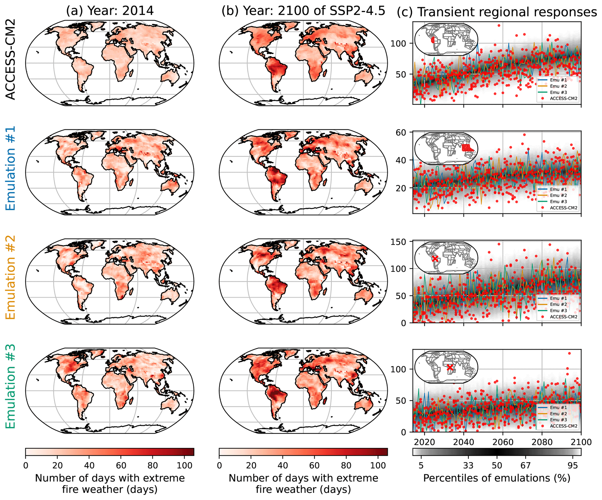
Figure A13Similar to Fig. 5 but with ACCESS-CM2 and the medium-warming scenario SSP2-4.5.
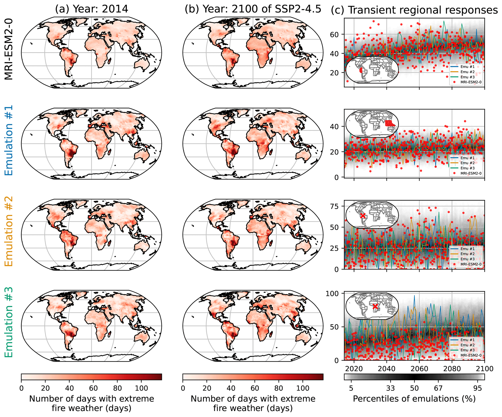
Figure A14Similar to Fig. 5 but with ACCESS-CM2 and the low-warming scenario SSP1-2.6.
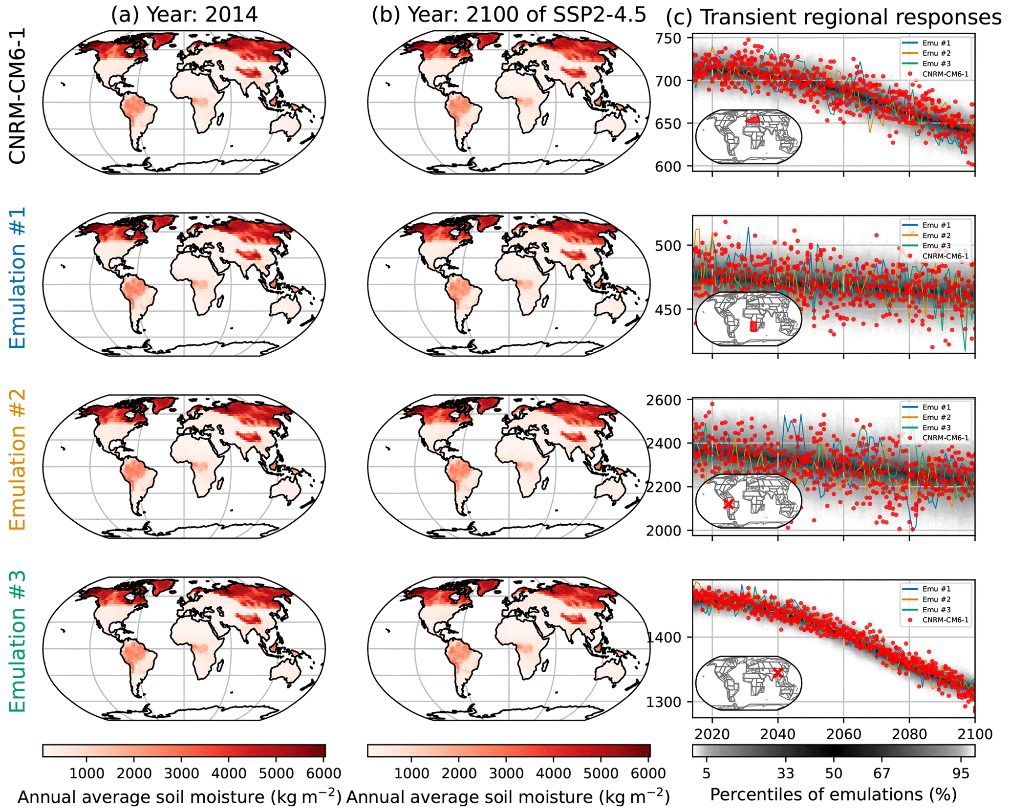
Figure A15Similar to Fig. 9 but with the medium-warming scenario SSP2-4.5.
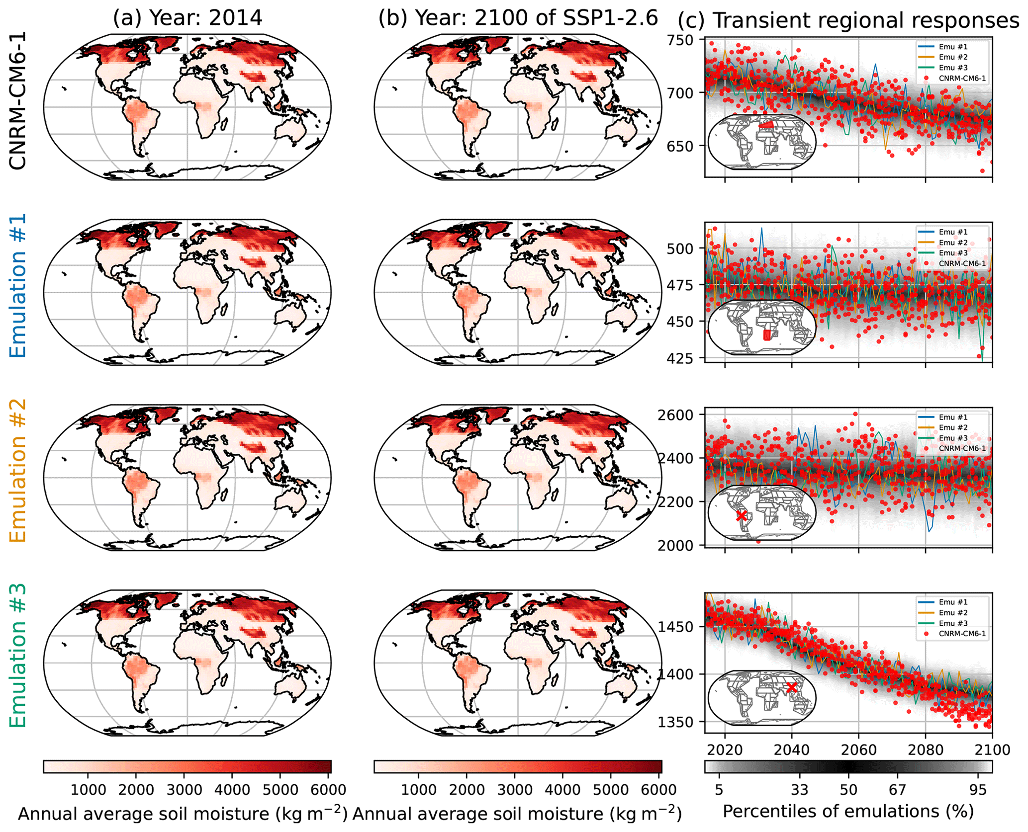
Figure A16Similar to Fig. 9 but with the low-warming scenario SSP1-2.6.
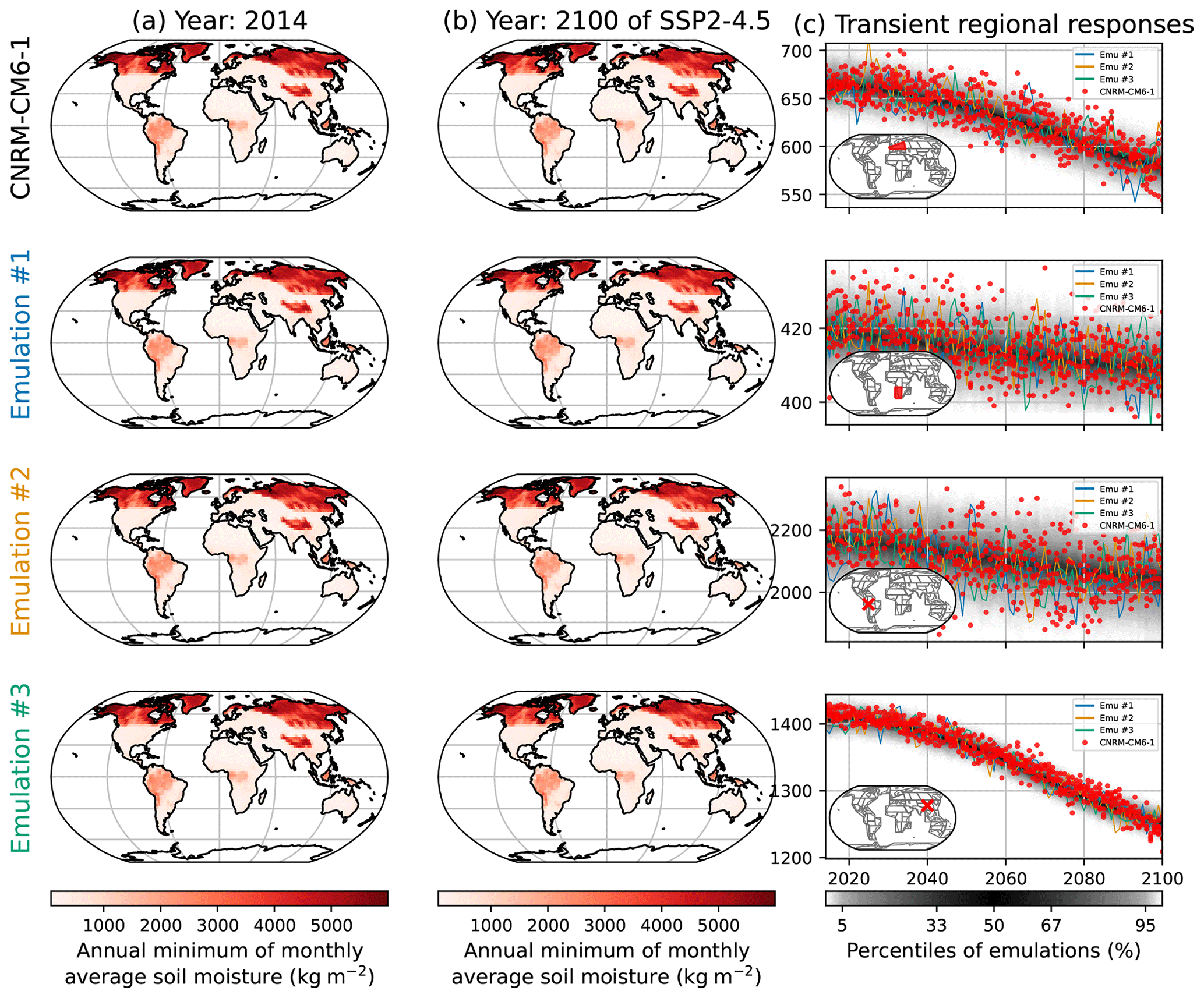
Figure A17Similar to Fig. 12 but with the medium-warming scenario SSP2-4.5.
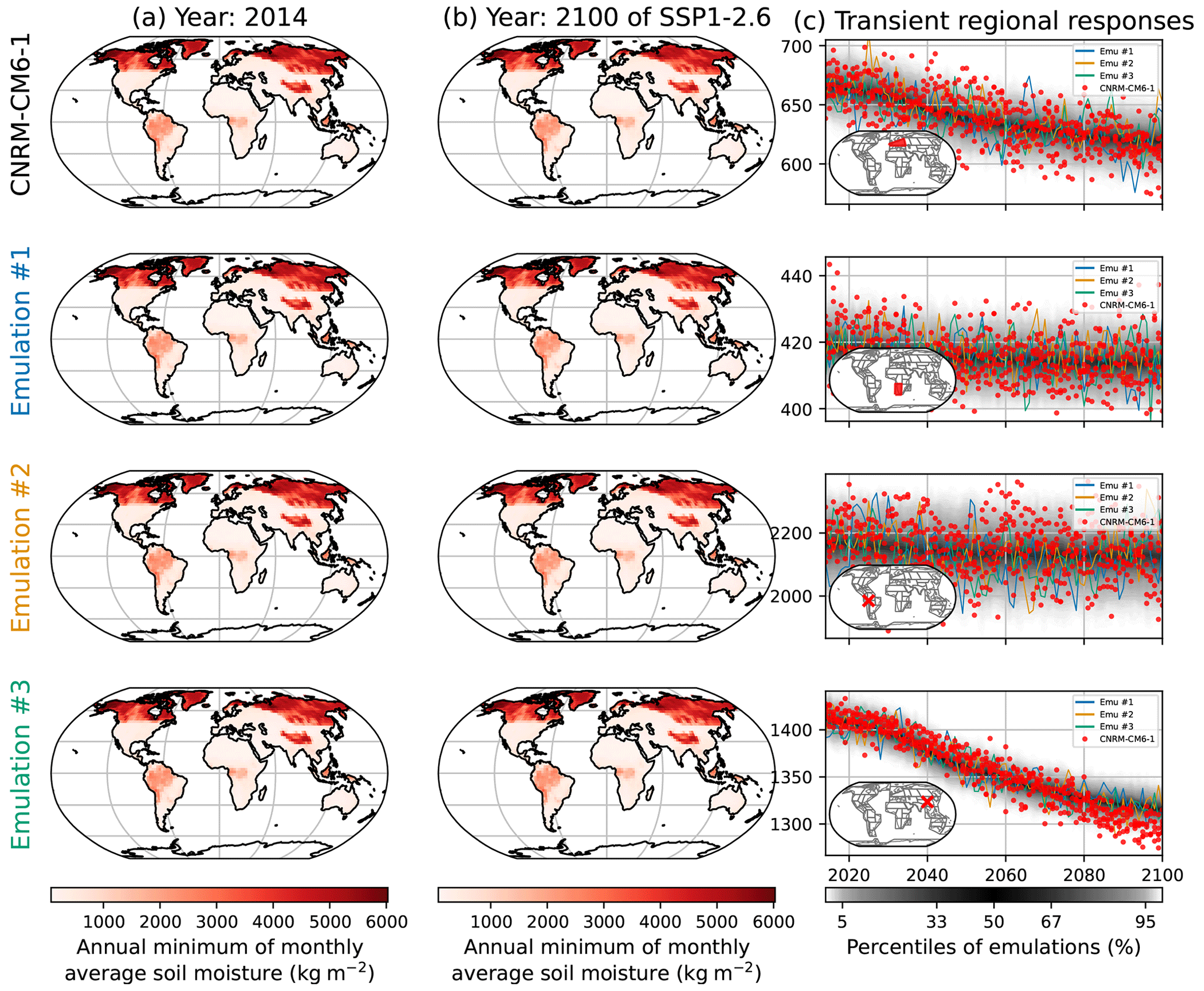
Figure A18Similar to Fig. 12 but with the low-warming scenario SSP1-2.6.
Data from CMIP6 can be accessed and downloaded at https://esgf-node.llnl.gov/search/cmip6/ (last access: 29 January 2023). The search query is as follows: experiment ID (historical, ssp119, ssp1226, ssp245, ssp370, ssp585, ssp534-over) and variable (tas, mrso). Code from MESMER is available at https://doi.org/10.5281/zenodo.10300296 (Quilcaille, 2023). Data for the FWI can be accessed at https://doi.org/10.3929/ethz-b-000583391 (Quilcaille and Batibeniz, 2022).
YQ, LG, and SIS conceptualized the study. YQ developed the software, carried out the analysis, and drafted the text. LG provided statistical support for the analysis. YQ, LG, and SIS contributed to interpreting the results and refining the text.
At least one of the (co-)authors is a member of the editorial board of Earth System Dynamics. The peer-review process was guided by an independent editor, and the authors also have no other competing interests to declare.
Publisher's note: Copernicus Publications remains neutral with regard to jurisdictional claims made in the text, published maps, institutional affiliations, or any other geographical representation in this paper. While Copernicus Publications makes every effort to include appropriate place names, the final responsibility lies with the authors.
We acknowledge the World Climate Research Program for the promotion and coordination of the exercise and the data of CMIP6 but also the climate modeling groups for their model outputs. We acknowledge the Earth System Grid Federation for archiving the data and providing access. We thank Urs Beyerle for downloading and curating the CMIP6 data. We thank Lukas Brunner for processing the data into the CMIP6-ng archive. We acknowledge funding from the European Research Council (ERC) through the ERC Proof-Of-Concept Grant MESMER-X (grant agreement no. 964013) and the PROVIDE project (grant agreement no. 101003687). We acknowledge as well the Swiss National Science Foundation (SNSF) through the Compound Events in a Changing Climate (CECC) (grant agreement no. IZCOZ0_189941). We thank the referee Claudia Tebaldi, the anonymous referee, and the handling editor Vivek Arora for their comments.
This research has been supported by the H2020 Excellent Science (grant no. 964013) and H2020 Societal Challenges (grant no. 101003687) programmes and the Schweizerischer Nationalfonds zur Förderung der Wissenschaftlichen Forschung (grant no. 189941).
This paper was edited by Vivek Arora and reviewed by Claudia Tebaldi and one anonymous referee.
Abatzoglou, J. T., Williams, A. P., Boschetti, L., Zubkova, M., and Kolden, C. A.: Global patterns of interannual climate–fire relationships, Glob. Change Biol., 24, 5164–5175, https://doi.org/10.1111/gcb.14405, 2018.
Abatzoglou, J. T., Williams, A. P., and Barbero, R.: Global Emergence of Anthropogenic Climate Change in Fire Weather Indices, Geophys. Res. Lett., 46, 326–336, https://doi.org/10.1029/2018GL080959, 2019.
Alexeeff, S. E., Nychka, D., Sain, S. R., and Tebaldi, C.: Emulating mean patterns and variability of temperature across and within scenarios in anthropogenic climate change experiments, Climatic Change, 146, 319–333, https://doi.org/10.1007/s10584-016-1809-8, 2018.
Allan, R. P., Barlow, M., Byrne, M. P., Cherchi, A., Douville, H., Fowler, H. J., Gan, T. Y., Pendergrass, A. G., Rosenfeld, D., Swann, A. L. S., Wilcox, L. J., and Zolina, O.: Advances in understanding large-scale responses of the water cycle to climate change, Ann. NY Acad. Sci., 1472, 49–75, https://doi.org/10.1111/nyas.14337, 2020.
Andela, N., Morton, D. C., Giglio, L., Chen, Y., van der Werf, G. R., Kasibhatla, P. S., DeFries, R. S., Collatz, G. J., Hantson, S., Kloster, S., Bachelet, D., Forrest, M., Lasslop, G., Li, F., Mangeon, S., Melton, J. R., Yue, C., and Randerson, J. T.: A human-driven decline in global burned area, Science, 356, 1356–1362, https://doi.org/10.1126/science.aal4108, 2017.
Anderson, K. and Peters, G.: The trouble with negative emissions, Science, 354, 182–183, https://doi.org/10.1126/science.aah4567, 2016.
Angus, J. E.: The probability integral transform and related results, SIAM Rev., 36, 652–654, 1994.
Bedia, J., Herrera, S., Gutiérrez, J. M., Benali, A., Brands, S., Mota, B., and Moreno, J. M.: Global patterns in the sensitivity of burned area to fire-weather: Implications for climate change, Agr. Forest Meteorol., 214–215, 369–379, https://doi.org/10.1016/j.agrformet.2015.09.002, 2015.
Beusch, L., Gudmundsson, L., and Seneviratne, S. I.: Emulating Earth system model temperatures with MESMER: from global mean temperature trajectories to grid-point-level realizations on land, Earth Syst. Dynam., 11, 139–159, https://doi.org/10.5194/esd-11-139-2020, 2020a.
Beusch, L., Gudmundsson, L., and Seneviratne, S. I.: Crossbreeding CMIP6 Earth System Models With an Emulator for Regionally Optimized Land Temperature Projections, Geophys. Res. Lett., 47, e2019GL086812, https://doi.org/10.1029/2019GL086812, 2020b.
Beusch, L., Nauels, A., Gudmundsson, L., Gütschow, J., Schleussner, C.-F., and Seneviratne, S. I.: Responsibility of major emitters for country-level warming and extreme hot years, Commun. Earth Environ., 3, 7, https://doi.org/10.1038/s43247-021-00320-6, 2022a.
Beusch, L., Nicholls, Z., Gudmundsson, L., Hauser, M., Meinshausen, M., and Seneviratne, S. I.: From emission scenarios to spatially resolved projections with a chain of computationally efficient emulators: coupling of MAGICC (v7.5.1) and MESMER (v0.8.3), Geosci. Model Dev., 15, 2085–2103, https://doi.org/10.5194/gmd-15-2085-2022, 2022b.
Brunner, L., Hauser, M., Lorenz, R., and Beyerle, U.: The ETH Zurich CMIP6 next generation archive: technical documentation (v1.0-final), Zenodo, https://doi.org/10.5281/zenodo.3734128, 2020.
Caretta, M. A., Mukherji, A., Arfanuzzaman, M., Betts, R. A., Gelfan, A., Hirabayashi, Y., Lissner, T. K., Liu, J., Lopez Gunn, E., Morgan, R., Mwanga, S., and Supratid, S.: Water, in: Climate Change 2022: Impacts, Adaptation and Vulnerability, Contribution of Working Group II to the Sixth Assessment Report of the Intergovernmental Panel on Climate Change, edited by: Pörtner, H.-O., Roberts, D. C., Tignor, M., Poloczanska, E. S., Mintenbeck, K., Alegriìa, A., Craig, M., Langsdorf, S., Löschke, S., Möller, V., Okem, A., and Rama, B. E., Cambridge University Press, https://doi.org/10.1017/9781009325844.006, 2022.
Carrassi, A., Bocquet, M., Bertino, L., and Evensen, G.: Data assimilation in the geosciences: An overview of methods, issues, and perspectives, WIREs Climate Change, 9, e535, https://doi.org/10.1002/wcc.535, 2018.
Coles, S.: An introduction to statistical modeling of extreme values, Springer, London, New York, https://doi.org/10.1007/978-1-4471-3675-0, 2001.
Cook, B. I., Mankin, J. S., Marvel, K., Williams, A. P., Smerdon, J. E., and Anchukaitis, K. J.: Twenty-First Century Drought Projections in the CMIP6 Forcing Scenarios, Earth's Future, 8, e2019EF001461, https://doi.org/10.1029/2019EF001461, 2020.
Cressie, N. and Wikle, C. K.: Statistics for spatio-temporal data, John Wiley & Sons, Hoboken, New Jersey, USA, 624 pp., ISBN 978-0-471-69274-4, 2011.
Douville, H., Raghavan, K., Renwick, J., Allan, R. P., Arias, P. A., Barlow, M., Cerezo-Mota, R., Cherchi, A., Gan, T. Y., Gergis, J., Jiang, D., Khan, A., Pokam Mba, W., Rosenfeld, D., Tierney, J., and Zolina, O.: Water Cycle Changes, in: Climate Change 2021: The Physical Science Basis, Contribution of Working Group I to the Sixth Assessment Report of the Intergovernmental Panel on Climate Change, edited by: Masson-Delmotte, V., Zhai, P., Pirani, A., Connors, S. L., Péan, C., Berger, S., Caud, N., Chen, Y., Goldfarb, L., Gomis, M. I., Huang, M., Leitzell, K., Lonnoy, E., Matthews, J. B. R., Maycock, T. K., Waterfield, T., Yelekçi, O., Yu, R., and Zhou, B. E., Cambridge University Press, https://doi.org/10.1017/9781009157896.010, 2021.
Eyring, V., Bony, S., Meehl, G. A., Senior, C. A., Stevens, B., Stouffer, R. J., and Taylor, K. E.: Overview of the Coupled Model Intercomparison Project Phase 6 (CMIP6) experimental design and organization, Geosci. Model Dev., 9, 1937–1958, https://doi.org/10.5194/gmd-9-1937-2016, 2016.
Friederichs, P. and Thorarinsdottir, T. L.: Forecast verification for extreme value distributions with an application to probabilistic peak wind prediction, Environmetrics, 23, 579–594, https://doi.org/10.1002/env.2176, 2012.
Fuss, S., Canadell, J. G., Peters, G. P., Tavoni, M., Andrew, R. M., Ciais, P., Jackson, R. B., Jones, C. D., Kraxner, F., Nakicenovic, N., Le Quéré, C., Raupach, M. R., Sharifi, A., Smith, P., and Yamagata, Y.: COMMENTARY: Betting on negative emissions, Nat. Clim. Change, 4, 850–853, 2014.
Gaspari, G. and Cohn, S. E.: Construction of correlation functions in two and three dimensions, Q. J. Roy. Meteor. Soc., 125, 723–757, https://doi.org/10.1002/qj.49712555417, 1999.
Gneiting, T., Balabdaoui, F., and Raftery, A. E.: Probabilistic forecasts, calibration and sharpness, J. Roy. Stat. Soc. B, 69, 243–268, https://doi.org/10.1111/j.1467-9868.2007.00587.x, 2007.
Greve, P., Gudmundsson, L., and Seneviratne, S. I.: Regional scaling of annual mean precipitation and water availability with global temperature change, Earth Syst. Dynam., 9, 227–240, https://doi.org/10.5194/esd-9-227-2018, 2018.
Grillakis, M., Voulgarakis, A., Rovithakis, A., Seiradakis, K. D., Koutroulis, A., Field, R. D., Kasoar, M., Papadopoulos, A., and Lazaridis, M.: Climate drivers of global wildfire burned area, Environ. Res. Lett., 17, 045021, https://doi.org/10.1088/1748-9326/ac5fa1, 2022.
Gudmundsson, L., Bremnes, J. B., Haugen, J. E., and Engen-Skaugen, T.: Technical Note: Downscaling RCM precipitation to the station scale using statistical transformations – a comparison of methods, Hydrol. Earth Syst. Sci., 16, 3383–3390, https://doi.org/10.5194/hess-16-3383-2012, 2012.
Hasegawa, T., Sakurai, G., Fujimori, S., Takahashi, K., Hijioka, Y., and Masui, T.: Extreme climate events increase risk of global food insecurity and adaptation needs, Nat. Food, 2, 587–595, https://doi.org/10.1038/s43016-021-00335-4, 2021.
Herger, N., Sanderson, B. M., and Knutti, R.: Improved pattern scaling approaches for the use in climate impact studies, Geophys. Res. Lett., 42, 3486–3494, https://doi.org/10.1002/2015GL063569, 2015.
Hersbach, H.: Decomposition of the Continuous Ranked Probability Score for Ensemble Prediction Systems, Weather Forecast., 15, 559–570, https://doi.org/10.1175/1520-0434(2000)015<0559:DOTCRP>2.0.CO;2, 2000.
Hoegh-Guldberg, O., Jacob, D., Taylor, M., Bindi, M., Brown, S., Camilloni, I., Diedhiou, A., Djalante, R., Ebi, K., Engelbrecht, F., Guiot, J., Hijioka, Y., Mehrotra, S., Payne, A., Seneviratne, S. I., Thomas, A., Warren, R., and Zhou, G.: Impacts of 1.5∘ C global warming on natural and human systems, in: Global warming of 1.5∘e C, An IPCC Special Report on the impacts of global warming of 1.5∘ C above pre-industrial levels and related global greenhouse gas emission pathways, in the context of strengthening the global response to the threat of climate change, sustainable development, and efforts to eradicate poverty, edited by: Masson-Delmotte, V., Zhai, P., Pörtner, H. O., Roberts, D., Skea, J., Shukla, P. R., Pirani, A., Moufouma-Okia, W., Péan, C., Pidcock, R., Connors, S., Matthews, J. B. R., Chen, Y., Zhou, X., Gomis, M. I., Lonnoy, E., Maycock, T., Tignor, M., and Waterfield, T., Cambridge University Press, Cambridge, UK and New York, NY, USA, 175–312, https://doi.org/10.1017/9781009157940.005, 2018.
Humphrey, V. and Gudmundsson, L.: GRACE-REC: a reconstruction of climate-driven water storage changes over the last century, Earth Syst. Sci. Data, 11, 1153–1170, https://doi.org/10.5194/essd-11-1153-2019, 2019.
IPCC: Field, C. B., Barros, V. R., Dokken, D. J., Mach, K. J., Mastrandrea, M. D., Bilir, T. E., Chatterjee, M., Ebi, K. L., Estrada, Y. O., Genova, R. C., Girma, B., Kissel, E. S., Levy, A. N., MacCracken, S., Mastrandrea, P. R., and White, L. L. (Eds.): Climate Change 2014: Impacts, Adaptation, and Vulnerability. Part A: Global and Sectoral Aspects. Contribution of Working Group II to the Fifth Assessment Report of the Intergovernmental Panel on Climate Change, Cambridge University Press, ISBN 978-1-107-05807-1, 2014.
IPCC: Global warming of 1.5C. An IPCC Special Report on the impacts of global warming of 1.5C above pre-industrial levels and related global greenhouse gas emission pathways, in the context of strengthening the global response to the threat of climate change, sustainable development, and efforts to eradicate poverty, Cambridge University Press, Cambridge, UK and New York, NY, USA, https://doi.org/10.1017/9781009157940, 2018.
Iturbide, M., Gutiérrez, J. M., Alves, L. M., Bedia, J., Cerezo-Mota, R., Cimadevilla, E., Cofiño, A. S., Di Luca, A., Faria, S. H., Gorodetskaya, I. V., Hauser, M., Herrera, S., Hennessy, K., Hewitt, H. T., Jones, R. G., Krakovska, S., Manzanas, R., Martínez-Castro, D., Narisma, G. T., Nurhati, I. S., Pinto, I., Seneviratne, S. I., van den Hurk, B., and Vera, C. S.: An update of IPCC climate reference regions for subcontinental analysis of climate model data: definition and aggregated datasets, Earth Syst. Sci. Data, 12, 2959–2970, https://doi.org/10.5194/essd-12-2959-2020, 2020.
Jain, P., Castellanos-Acuna, D., Coogan, S. C. P., Abatzoglou, J. T., and Flannigan, M. D.: Observed increases in extreme fire weather driven by atmospheric humidity and temperature, Nat. Clim. Change, 12, 63–70, https://doi.org/10.1038/s41558-021-01224-1, 2022.
Jolliffe, I. T. and Stephenson, D. B.: Forecast verification: a practitioner's guide in atmospheric science, John Wiley & Sons, https://doi.org/10.1002/9781119960003, 2012.
Jolly, W. M., Cochrane, M. A., Freeborn, P. H., Holden, Z. A., Brown, T. J., Williamson, G. J., and Bowman, D. M. J. S.: Climate-induced variations in global wildfire danger from 1979 to 2013, Nat. Commun., 6, 7537, https://doi.org/10.1038/ncomms8537, 2015.
Jones, M. W., Abatzoglou, J. T., Veraverbeke, S., Andela, N., Lasslop, G., Forkel, M., Smith, A. J. P., Burton, C., Betts, R. A., van der Werf, G. R., Sitch, S., Canadell, J. G., Santín, C., Kolden, C., Doerr, S. H., and Le Quéré, C.: Global and Regional Trends and Drivers of Fire Under Climate Change, Rev. Geophys., 60, e2020RG000726, https://doi.org/10.1029/2020RG000726, 2022.
Jones, P. W.: First- and Second-Order Conservative Remapping Schemes for Grids in Spherical Coordinates, Mon. Weather Rev., 127, 2204–2210, https://doi.org/10.1175/1520-0493(1999)127<2204:FASOCR>2.0.CO;2, 1999.
Kim, Y.-H., Min, S.-K., Zhang, X., Sillmann, J., and Sandstad, M.: Evaluation of the CMIP6 multi-model ensemble for climate extreme indices, Weather and Climate Extremes, 29, 100269, https://doi.org/10.1016/j.wace.2020.100269, 2020.
Li, F., Val Martin, M., Andreae, M. O., Arneth, A., Hantson, S., Kaiser, J. W., Lasslop, G., Yue, C., Bachelet, D., Forrest, M., Kluzek, E., Liu, X., Mangeon, S., Melton, J. R., Ward, D. S., Darmenov, A., Hickler, T., Ichoku, C., Magi, B. I., Sitch, S., van der Werf, G. R., Wiedinmyer, C., and Rabin, S. S.: Historical (1700–2012) global multi-model estimates of the fire emissions from the Fire Modeling Intercomparison Project (FireMIP), Atmos. Chem. Phys., 19, 12545–12567, https://doi.org/10.5194/acp-19-12545-2019, 2019.
Libonati, R., Geirinhas, J. L., Silva, P. S., Monteiro dos Santos, D., Rodrigues, J. A., Russo, A., Peres, L. F., Narcizo, L., Gomes, M. E. R., Rodrigues, A. P., DaCamara, C. C., Pereira, J. M. C., and Trigo, R. M.: Drought–heatwave nexus in Brazil and related impacts on health and fires: A comprehensive review, Ann. NY Acad. Sci., 1517, 44–62, https://doi.org/10.1111/nyas.14887, 2022.
Link, R., Snyder, A., Lynch, C., Hartin, C., Kravitz, B., and Bond-Lamberty, B.: Fldgen v1.0: an emulator with internal variability and space–time correlation for Earth system models, Geosci. Model Dev., 12, 1477–1489, https://doi.org/10.5194/gmd-12-1477-2019, 2019.
Liu, G., Peng, S., Huntingford, C., and Xi, Y.: A new precipitation emulator (PREMU v1.0) for lower-complexity models, Geosci. Model Dev., 16, 1277–1296, https://doi.org/10.5194/gmd-16-1277-2023, 2023.
Lüthi, S., Aznar-Siguan, G., Fairless, C., and Bresch, D. N.: Globally consistent assessment of economic impacts of wildfires in CLIMADA v2.2, Geosci. Model Dev., 14, 7175–7187, https://doi.org/10.5194/gmd-14-7175-2021, 2021.
Meinshausen, M., Raper, S. C. B., and Wigley, T. M. L.: Emulating coupled atmosphere-ocean and carbon cycle models with a simpler model, MAGICC6 – Part 1: Model description and calibration, Atmos. Chem. Phys., 11, 1417–1456, https://doi.org/10.5194/acp-11-1417-2011, 2011.
Nath, S., Lejeune, Q., Beusch, L., Seneviratne, S. I., and Schleussner, C.-F.: MESMER-M: an Earth system model emulator for spatially resolved monthly temperature, Earth Syst. Dynam., 13, 851–877, https://doi.org/10.5194/esd-13-851-2022, 2022.
Nath, S., Gudmundsson, L., Schwaab, J., Duveiller, G., De Hertog, S. J., Guo, S., Havermann, F., Luo, F., Manola, I., Pongratz, J., Seneviratne, S. I., Schleussner, C. F., Thiery, W., and Lejeune, Q.: TIMBER v0.1: a conceptual framework for emulating temperature responses to tree cover change, Geosci. Model Dev., 16, 4283–4313, https://doi.org/10.5194/gmd-16-4283-2023, 2023.
Nicholls, Z., Meinshausen, M., Lewis, J., Corradi, M. R., Dorheim, K., Gasser, T., Gieseke, R., Hope, A. P., Leach, N. J., McBride, L. A., Quilcaille, Y., Rogelj, J., Salawitch, R. J., Samset, B. H., Sandstad, M., Shiklomanov, A., Skeie, R. B., Smith, C. J., Smith, S. J., Su, X., Tsutsui, J., Vega-Westhoff, B., and Woodard, D. L.: Reduced Complexity Model Intercomparison Project Phase 2: Synthesising Earth system knowledge for probabilistic climate projections, Earth's Future, 9, e2020EF001900, https://doi.org/10.1029/2020EF001900, 2021.
Nicholls, Z. R. J., Meinshausen, M., Lewis, J., Gieseke, R., Dommenget, D., Dorheim, K., Fan, C.-S., Fuglestvedt, J. S., Gasser, T., Golüke, U., Goodwin, P., Hartin, C., Hope, A. P., Kriegler, E., Leach, N. J., Marchegiani, D., McBride, L. A., Quilcaille, Y., Rogelj, J., Salawitch, R. J., Samset, B. H., Sandstad, M., Shiklomanov, A. N., Skeie, R. B., Smith, C. J., Smith, S., Tanaka, K., Tsutsui, J., and Xie, Z.: Reduced Complexity Model Intercomparison Project Phase 1: introduction and evaluation of global-mean temperature response, Geosci. Model Dev., 13, 5175–5190, https://doi.org/10.5194/gmd-13-5175-2020, 2020.
O'Neill, B. C., Tebaldi, C., van Vuuren, D. P., Eyring, V., Friedlingstein, P., Hurtt, G., Knutti, R., Kriegler, E., Lamarque, J.-F., Lowe, J., Meehl, G. A., Moss, R., Riahi, K., and Sanderson, B. M.: The Scenario Model Intercomparison Project (ScenarioMIP) for CMIP6, Geosci. Model Dev., 9, 3461–3482, https://doi.org/10.5194/gmd-9-3461-2016, 2016.
Perera, A. T. D., Nik, V. M., Chen, D., Scartezzini, J.-L., and Hong, T.: Quantifying the impacts of climate change and extreme climate events on energy systems, Nature Energy, 5, 150–159, https://doi.org/10.1038/s41560-020-0558-0, 2020.
Qiao, L., Zuo, Z., and Xiao, D.: Evaluation of Soil Moisture in CMIP6 Simulations, J. Climate, 35, 779–800, https://doi.org/10.1175/JCLI-D-20-0827.1, 2022
Quilcaille, Y.: Code for “Extending MESMER-X: A spatially resolved Earth system model emulator for fire weather and soil moisture” (v1.0), Zenodo [code], https://doi.org/10.5281/zenodo.10300296, 2023.
Quilcaille, Y. and Batibeniz, F.: Fire weather index data under historical and SSP projections in CMIP6 from 1850 to 2100, ETH Bibliography [data set], https://doi.org/10.3929/ethz-b-000583391, 2022.
Quilcaille, Y., Gudmundsson, L., Beusch, L., Hauser, M., and Seneviratne, S. I.: Showcasing MESMER-X: Spatially Resolved Emulation of Annual Maximum Temperatures of Earth System Models, Geophys. Res. Lett., 49, e2022GL099012, https://doi.org/10.1029/2022GL099012, 2022.
Quilcaille, Y., Batibeniz, F., Ribeiro, A. F. S., Padrón, R. S., and Seneviratne, S. I.: Fire weather index data under historical and shared socioeconomic pathway projections in the 6th phase of the Coupled Model Intercomparison Project from 1850 to 2100, Earth Syst. Sci. Data, 15, 2153–2177, https://doi.org/10.5194/essd-15-2153-2023, 2023.
Ranasinghe, R., Ruane, A. C., Vautard, R., Arnell, N., Coppola, E., Cruz, F. A., Dessai, S., Islam, A. S., Rahimi, M., Ruiz Carrascal, D., Sillmann, J., Sylla, M. B., Tebaldi, C., Wang, W., and Zaaboul, R.: Climate Change Information for Regional Impact and for Risk Assessment, in: Climate Change 2021: The Physical Science Basis. Contribution of Working Group I to the Sixth Assessment Report of the Intergovernmental Panel on Climate Change, edited by: Masson-Delmotte, V., Zhai, P., Pirani, A., Connors, S. L., Péan, C., Berger, S., Caud, N., Chen, Y., Goldfarb, L., Gomis, M. I., Huang, M., Leitzell, K., Lonnoy, E., Matthews, J. B. R., Maycock, T. K., Waterfield, T., Yelekçi, O., Yu, R., and Zhou, B., Cambridge University Press, Cambridge, United Kingdom and New York, NY, USA, 1767–1926, https://doi.org/10.1017/9781009157896.014, 2021.
Ribeiro, A. F. S., Brando, P. M., Santos, L., Rattis, L., Hirschi, M., Hauser, M., Seneviratne, S. I., and Zscheischler, J.: A compound event-oriented framework to tropical fire risk assessment in a changing climate, Environ. Res. Lett., 17, 065015, https://doi.org/10.1088/1748-9326/ac7342, 2022.
Schaeffer, R., Szklo, A. S., Pereira de Lucena, A. F., Moreira Cesar Borba, B. S., Pupo Nogueira, L. P., Fleming, F. P., Troccoli, A., Harrison, M., and Boulahya, M. S.: Energy sector vulnerability to climate change: A review, Energy, 38, 1–12, https://doi.org/10.1016/j.energy.2011.11.056, 2012.
Schewe, J., Gosling, S. N., Reyer, C., Zhao, F., Ciais, P., Elliott, J., Francois, L., Huber, V., Lotze, H. K., Seneviratne, S. I., van Vliet, M. T. H., Vautard, R., Wada, Y., Breuer, L., Büchner, M., Carozza, D. A., Chang, J., Coll, M., Deryng, D., de Wit, A., Eddy, T. D., Folberth, C., Frieler, K., Friend, A. D., Gerten, D., Gudmundsson, L., Hanasaki, N., Ito, A., Khabarov, N., Kim, H., Lawrence, P., Morfopoulos, C., Müller, C., Müller Schmied, H., Orth, R., Ostberg, S., Pokhrel, Y., Pugh, T. A. M., Sakurai, G., Satoh, Y., Schmid, E., Stacke, T., Steenbeek, J., Steinkamp, J., Tang, Q., Tian, H., Tittensor, D. P., Volkholz, J., Wang, X., and Warszawski, L.: State-of-the-art global models underestimate impacts from climate extremes, Nat. Commun., 10, 1005, https://doi.org/10.1038/s41467-019-08745-6, 2019.
Seneviratne, S. I., Zhang, X., Adnan, M., Badi, W., Dereczynski, C., Di Luca, A., Ghosh, S., Iskandar, I., Kossin, J., Lewis, S., Otto, F., Pinto, I., Satoh, M., Vicente-Serrano, S. M., Wehner, M., and Zhou, B.: Weather and Climate Extreme Events in a Changing Climate, in: Climate Change 2021: The Physical Science Basis. Contribution of Working Group I to the Sixth Assessment Report of the Intergovernmental Panel on Climate Change, edited by: Masson-Delmotte, V., Zhai, P., Pirani, A., Connors, S. L., Péan, C., Berger, S., Caud, N., Chen, Y., Goldfarb, L., Gomis, M. I., Huang, M., Leitzell, K., Lonnoy, E., Matthews, J. B. R., Maycock, T. K., Waterfield, T., Yelekçi, O., Yu, R., and Zhou, B. E., Cambridge University Press, https://doi.org/10.1017/9781009157896.013, 2021.
Smith, P., Davis, S. J., Creutzig, F., Fuss, S., Minx, J., Gabrielle, B., Kato, E., Jackson, R. B., Cowie, A., Kriegler, E., Van Vuuren, D. P., Rogelj, J., Ciais, P., Milne, J., Canadell, J. G., McCollum, D., Peters, G., Andrew, R., Krey, V., Shrestha, G., Friedlingstein, P., Gasser, T., Grubler, A., Heidug, W. K., Jonas, M., Jones, C. D., Kraxner, F., Littleton, E., Lowe, J., Moreira, J. R., Nakicenovic, N., Obersteiner, M., Patwardhan, A., Rogner, M., Rubin, E., Sharifi, A., Torvanger, A., Yamagata, Y., Edmonds, J., and Yongsung, C,: Biophysical and economic limits to negative CO2 emissions, Nat. Clim. Change, 6, 42–50, 2016.
Stehfest, E., van Vuuren, D., Kram, T., Bouwman, L., Alkemade, R., Bakkenes, M., Biemans, H., Bouwman, A., den Elzen, M., Janse, J., Lucas, P., van Minnen, J., Müller, M., and Prins, A.: Integrated Assessment of Global Environmental Change with IMAGE 3.0: Model description and policy applications, 336 pp., ISBN 978-94-91506-71-0, 2014.
Tebaldi, C. and Arblaster, J. M.: Pattern scaling: Its strengths and limitations, and an update on the latest model simulations, Climatic Change, 122, 459–471, https://doi.org/10.1007/s10584-013-1032-9, 2014.
Tebaldi, C., Armbruster, A., Engler, H. P., and Link, R.: Emulating climate extreme indices, Environ. Res. Lett., 15, 074006, https://doi.org/10.1088/1748-9326/ab8332, 2020.
Tebaldi, C., Snyder, A., and Dorheim, K.: STITCHES: creating new scenarios of climate model output by stitching together pieces of existing simulations, Earth Syst. Dynam., 13, 1557–1609, https://doi.org/10.5194/esd-13-1557-2022, 2022.
van den Hurk, B., Kim, H., Krinner, G., Seneviratne, S. I., Derksen, C., Oki, T., Douville, H., Colin, J., Ducharne, A., Cheruy, F., Viovy, N., Puma, M. J., Wada, Y., Li, W., Jia, B., Alessandri, A., Lawrence, D. M., Weedon, G. P., Ellis, R., Hagemann, S., Mao, J., Flanner, M. G., Zampieri, M., Materia, S., Law, R. M., and Sheffield, J.: LS3MIP (v1.0) contribution to CMIP6: the Land Surface, Snow and Soil moisture Model Intercomparison Project – aims, setup and expected outcome, Geosci. Model Dev., 9, 2809–2832, https://doi.org/10.5194/gmd-9-2809-2016, 2016.
van Oldenborgh, G. J., Krikken, F., Lewis, S., Leach, N. J., Lehner, F., Saunders, K. R., van Weele, M., Haustein, K., Li, S., Wallom, D., Sparrow, S., Arrighi, J., Singh, R. K., van Aalst, M. K., Philip, S. Y., Vautard, R., and Otto, F. E. L.: Attribution of the Australian bushfire risk to anthropogenic climate change, Nat. Hazards Earth Syst. Sci., 21, 941–960, https://doi.org/10.5194/nhess-21-941-2021, 2021.
Van Wagner, C. E.: Development and structure of the Canadian forest fire weather index system, Canadian Forestry Service, Ottawa, ISBN 0-662-15198-4, 1987.
Vogel, E., Donat, M. G., Alexander, L. V., Meinshausen, M., Ray, D. K., Karoly, D., Meinshausen, N., and Frieler, K.: The effects of climate extremes on global agricultural yields, Environ. Res. Lett., 14, 054010, https://doi.org/10.1088/1748-9326/ab154b, 2019.
von Buttlar, J., Zscheischler, J., Rammig, A., Sippel, S., Reichstein, M., Knohl, A., Jung, M., Menzer, O., Arain, M. A., Buchmann, N., Cescatti, A., Gianelle, D., Kiely, G., Law, B. E., Magliulo, V., Margolis, H., McCaughey, H., Merbold, L., Migliavacca, M., Montagnani, L., Oechel, W., Pavelka, M., Peichl, M., Rambal, S., Raschi, A., Scott, R. L., Vaccari, F. P., van Gorsel, E., Varlagin, A., Wohlfahrt, G., and Mahecha, M. D.: Impacts of droughts and extreme-temperature events on gross primary production and ecosystem respiration: a systematic assessment across ecosystems and climate zones, Biogeosciences, 15, 1293–1318, https://doi.org/10.5194/bg-15-1293-2018, 2018.
Wang, Q., Wu, J., Lei, T., He, B., Wu, Z., Liu, M., Mo, X., Geng, G., Li, X., Zhou, H., and Liu, D.: Temporal-spatial characteristics of severe drought events and their impact on agriculture on a global scale, Quatern. Int., 349, 10–21, https://doi.org/10.1016/j.quaint.2014.06.021, 2014.
Watson-Parris, D., Rao, Y., Olivié, D., Seland, Ø., Nowack, P., Camps-Valls, G., Stier, P., Bouabid, S., Dewey, M., Fons, E., Gonzalez, J., Harder, P., Jeggle, K., Lenhardt, J., Manshausen, P., Novitasari, M., Ricard, L., and Roesch, C.: ClimateBench v1.0: A Benchmark for Data-Driven Climate Projections, J. Adv. Model. Earth Sy., 14, e2021MS002954, https://doi.org/10.1029/2021MS002954, 2022.
Wiebe, K., Lotze-Campen, H., Sands, R., Tabeau, A., van der Mensbrugghe, D., Biewald, A., Bodirsky, B., Islam, S., Kavallari, A., Mason-D'Croz, D., Müller, Christoph, Popp, A., Robertson, R., Robinson, S., van Meijl, H., and Willenbockel, D.: Climate change impacts on agriculture in 2050 under a range of plausible socioeconomic and emissions scenarios, Environ. Res. Lett., 10, 085010, https://doi.org/10.1088/1748-9326/10/8/085010, 2015.
Wilks, D. S. (Ed.): Statistical methods in the atmospheric sciences, 100, 2–676, ISBN 978-0-12-385022-5, 2011.