The Indonesian Throughflow circulation under solar geoengineering

The Indonesia Throughflow (ITF) is the only low-latitude channel between the Pacific and Indian oceans, and its variability has important effects on global climate and biogeochemical cycles. Climate models consistently predict a decline in ITF transport under global warming, but it has not yet been examined under solar geoengineering scenarios. We use standard parameterized methods for estimating the ITF – the Amended Island Rule and buoyancy forcing – to investigate the ITF under the SSP2-4.5 and SSP5-8.5 greenhouse gas scenarios and the geoengineering experiments G6solar and G6sulfur, which reduce net global mean radiative forcing from SSP5-8.5 levels to SSP2-4.5 levels using solar dimming and sulfate aerosol injection strategies, respectively. Six-model ensemble-mean projections for 2080–2100 show reductions of 19 % under the G6solar scenario and 28 % under the G6sulfur scenario relative to the historical (1980–2014) ITF, which should be compared with reductions of 23 % and 27 % under SSP2-4.5 and SSP5-8.5. Despite standard deviations amounting to 5 %–8 % for each scenario, all scenarios are significantly different from each other (p<0.05) when the whole 2020–2100 simulation period is considered. Thus, significant weakening of the ITF occurs under all scenarios, but G6solar more closely approximates SSP2-4.5 than G6sulfur does. In contrast with the other three scenarios, which show only reductions in forcing due to ocean upwelling, the G6sulfur experiment shows a large reduction in ocean surface wind stress forcing accounting for 47 % (38 %–65 % across the model range) of the decline in wind + upwelling-driven ITF transport. There are also reductions in deep-sea upwelling in extratropical western boundary currents.

1 Introduction

The Indonesian Throughflow (ITF) is an important part of the global thermohaline circulation (Gordon, 1986; Lee et al., 2002; Sprintall et al., 2009). The ITF brings about 15 Sv (∼10.7 to ∼18.7 Sv during the INSTANT Field Program, 2004–2006; 1 Sv = 10⁶ m³ s⁻¹) of warm and fresh water from the Pacific to the Indian Ocean (Sprintall et al., 2009). Since the ITF is the only ocean pathway in the tropics between the Pacific and Indian oceans, it is key to the heat and water volume transport between them (Godfrey, 1996; Talley, 2008). The ITF also plays an important role in regulating global climate and biogeochemical cycles (Ayers et al., 2014; Hirst and Godfrey, 1994) – for example, the ITF may influence the El Niño–Southern Oscillation (ENSO) by altering the tropical–subtropical exchange, the structure of the mean tropical thermocline, and the mean sea surface temperature (SST) difference between the Pacific Warm Pool and the Cold Tongue, etc. (Lee et al., 2002) – and in the supply of iron in the equatorial upwelling, thus maintaining biological production in the equatorial eastern Pacific (Gorgues et al., 2007). Sen Gupta et al. (2021) used 26 CMIP6 models to predict an ITF weakening of 3 Sv (2.4–3.2 Sv model range) under the SSP5-8.5 scenario (the high greenhouse gas emission scenario) relative to 20th century historical means. The decline in the ITF would cause more heat to accumulate in the Pacific Ocean, which could alter tropical atmosphere–ocean interactions and contribute to extreme El Niño/La Niña events (Cai et al., 2015; Klinger and Garuba, 2016).

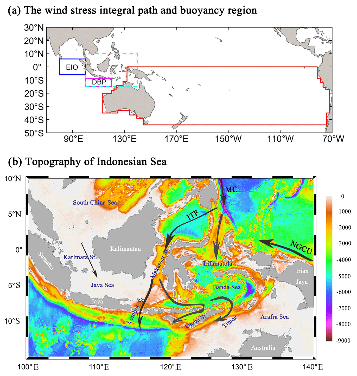
Figure 1 (a) The wind stress integral path for the Island Rule (red line), the Downstream Buoyant Pool (magenta box), and the Equatorial Indian Ocean (blue box), where the density difference is the main index used to calculate the ITF transport by buoyancy forcing. (b) Inset defined by the dotted cyan line in (a). This shows the offshore bathymetry in the Maritime Continent (ETOPO Global Relief Model; Amante and Eakins, 2009), the Mindanao Current (MC), and the New Guinea Coast Undercurrent (NGCU) paths that contribute to the ITF.

The ITF is fed by the Mindanao Current, the New Guinea Coast Undercurrent (Fig. 1), and, to a lesser extent, parts of the low-latitude Pacific Western Boundary Current (WBC) that flows toward the Equator (Godfrey, 1996; Lukas et al., 1996). The ITF helps supply the Agulhas Current leakage from the Indian Ocean to the South Atlantic Ocean, and may be said to flush Indian Ocean thermocline waters southward by boosting the Agulhas Current (Durgadoo et al., 2017; Gordon, 2005).

The interannual and decadal variability of ITF transport is influenced by surface winds in the Pacific and Indian oceans (Feng et al., 2011; Meyers, 1996). Wyrtki (1987) noticed that the pressure gradient between the Pacific and Indian oceans dominates the ITF flux and hence that the sea level is a good indicator of upper-ocean ITF transport. The largest volume flux occurs in July–August and the lowest in January–February.

Model simulations consistently project that ITF transport will be weakened by increased greenhouse gas (GHG) forcing (Feng et al., 2012; Hu et al., 2015; Sen Gupta et al., 2021; Vecchi and Soden, 2007). The driving force is the weakening of the Pacific trade winds under global warming in the 21st century, which then weaken the Mindanao Current, the main inflow route of the ITF (Alory et al., 2007; Duan et al., 2017; Sen Gupta et al., 2012).

Analyzing the water flux through the many shallow channels in the Indonesian archipelago is challenging, and many of these channels are not resolved in simulations with resolutions of a degree or so (Gordon et al., 1999) (Fig. 1). This motivates the use of alternative methods of estimating the ITF. Godfrey (1989) created the Island Rule to estimate the flux based on Sverdrup's theoretical analysis of Pacific wind stress (Sverdrup, 1947). More recently, the analysis of climate models has revealed the importance of deep ocean circulation to the reduction in ITF transport under GHG forcing. The decline in the ITF under GHG forcing could be due to both the weakening of trade winds in the Pacific and deep ocean circulation changes (Feng et al., 2012; Hu et al., 2015). An interannual to decadal as well as a centennial dependence of the ITF on wind and upwelling was found with an eddy-resolving ocean model simulation (Feng et al., 2017). This led to Sen Gupta et al. (2016) and Feng et al. (2017) proposing the Amended Island Rule that modifies the Island Rule to include the estimated net Pacific upwelling contribution to the ITF based on high-resolution ($\mathrm{1}/{\mathrm{10}}^{\circ }$) ocean general circulation modeling.

An alternative mechanism for the ITF driver was proposed earlier by Andersson and Stigebrandt (2005). In this theory, buoyancy forcing is more important than wind forcing in driving the ITF. The ITF variability is found from the baroclinic outflow of the Downstream Buoyant Pool (DBP) that extends over much of the North Australian Basin (Fig. 1). Hu and Sprintall (2016) used this method with reanalysis products to produce an ITF interannual variability that was in good agreement with the observed volume transports (2004–2006) from the INSTANT mooring array transport (Sprintall et al., 2009), although the average transport was only half the transport observed during INSTANT. INSTANT uses moorings deployed at the major inflow (Makassar Strait and Lifamatola Strait) and outflow (Lombok Strait, Ombai Strait, and Timor Passage) passages of the ITF to estimate the ITF transport, resulting in a value of 15 Sv during 2004–2006. Compared with the reasonable agreement for the Amended Island Rule estimates of ITF, the alternative “buoyancy” method behaves much worse, indicating that the hypothetical forcing is not as good an explanation for the ITF as the Amended Island Rule or that the models used do not capture the specific details of the DBP. But, although the Amended Island Rule matches the short duration of observed fluxes and variability better than buoyancy, it is possible that changes in buoyancy forcing may affect the volume transport of the ITF on decadal scales under a changing climate, and so we examine its changes under the geoengineering scenarios.

Solar radiation modification (SRM) geoengineering is designed to reduce the solar radiation reaching the surface of the earth and to slow down climate warming due to GHG forcing (Shepherd, 2009). Since SRM shortwave forcing has a different spatial and temporal variability than longwave forcing, it can only imperfectly offset the climate change caused by the increase in GHGs. In this article, we focus on two styles of SRM: the reduction of the solar constant to mimic the effect of a sunshade, called solar dimming (SD); and stratospheric aerosol injection (SAI), specifically involving the injection of sulfate aerosol into the tropical lower stratosphere (Kravitz et al., 2015). These styles of SRM are known to produce overcooled tropical oceans and undercooled poles relative to global mean temperatures. However, injection strategies other than the simple tropical site specified by G6 can produce simulated climates without these temperature biases (MacMartin and Kravitz, 2016). Simulated tropical atmospheric circulation systems are impacted under both GHG and solar geoengineering scenarios. Under SD, the seasonal movement of the Intertropical Convergence Zone is reduced relative to GHG climates (Smyth et al., 2017). Both the Hadley and Walker circulations are different from the historical ones (Cheng et al., 2022; Guo et al., 2018). The impacts of SRM on the Walker circulation are modest compared with those on Hadley cells, but they are most obvious in relation to the South Pacific Convergence Zone (Guo et al., 2018), which is relevant in the overall tropical Pacific atmosphere system that drives and interacts with the ITF. Greenhouse gas forcing is expected to cause an expansion of the Hadley circulation cells, which may be asymmetric between the Northern and Southern hemispheres (Staten et al., 2019). Both SD (Guo et al., 2018) and SAI (Cheng et al., 2022) reduce these greenhouse-gas-induced changes in the Hadley circulation, although, again, hemispheric differences remain, and in the simulations by Cheng et al. (2022) they were associated with stratospheric heating and a tropospheric temperature response due to enhanced stratospheric aerosol concentrations. The changes in stratospheric heating, the tropopause height, and tropical sea surface temperatures may be expected to impact tropical cyclogenesis, and this is consistent with reductions in the number and intensities of North Atlantic hurricanes relative to GHG-only climates under SAI (Moore et al., 2015). However, there are differences between tropical basins in expected tropical cyclogenesis potential and significant differences in simulations between climate models (Wang et al., 2018). The potential energy available for extratropical storms is also consistently reduced under SRM relative to GHG forcing (Gertler et al., 2020). The reported impacts highlight the potential role of wind forcing in the ITF.

To date, little research has been done on the ocean circulation under SRM, with only the Atlantic Meridional Overturning Circulation (AMOC) studied in depth (Hong et al., 2017; Moore et al., 2019; Muri et al., 2018; Tilmes et al., 2020; Xie et al., 2022). Both GHG forcing alone and with SRM produce a weakening of the AMOC relative to the present day, mainly in response to the change in heat flux in the North Atlantic, with little influence of the changes in freshwater flux and wind stress (Hong et al., 2017; Xie et al., 2022). The AMOC is less weakened under SRM than with GHG forcing alone, and the AMOC declines seen under GHG forcing are consistently reversed by SRM towards present day patterns (Moore et al., 2019; Muri et al., 2018; Tilmes et al., 2020).

In this study, we examine the impact of SRM on the change in the ITF in the 21st century, and we consider the transport and driver differences between pure GHG climates representing moderate mitigation (SSP2-4.5) and no mitigation (SSP5-8.5) along with solar dimming (G6solar) and stratospheric aerosol injection (G6sulfur) as forms of SRM geoengineering.

2 Climate models and scenarios

The Intergovernmental Panel on Climate Change (IPCC) Shared Socioeconomic Pathways (SSPs) are scenarios defined by radiative forcing goals to be achieved through various climate mitigation policy alternatives (Kriegler et al., 2012; van Vuuren et al., 2011). The climate model simulations under the SSPs are being performed as part of the Coupled Model Intercomparison Project Phase 6 (CMIP6). We used the CMIP6 historical simulation for 1980–2014 (Eyring et al., 2016) and two GHG scenarios for 2015–2100: SSP5-8.5, an unmitigated GHG emission scenario which raises the mean global radiative forcing by 8.5 W m⁻² over pre-industrial levels at 2100; and SSP2-4.5, which is designed to reach a peak radiative forcing of 4.5 W m⁻² by mid-century (O'Neill et al., 2016). We used the Geoengineering Model Intercomparison Project Phase 6 (GeoMIP6) G6sulfur and G6solar scenarios for 2020–2100 (Kravitz et al., 2015). The G6sulfur experiment specifies the use of SAI to reduce the net anthropogenic radiative forcing constantly during the 2020–2100 period from the SSP5-8.5 to the SSP2-4.5 level, while G6solar does the same using SD (Kravitz et al., 2015). The two SRM methods produce significantly different surface climates, with differences from SSP2-4.5 being larger and more spatially variable under G6sulfur than G6solar (Visioni et al., 2021). While the G6 scenarios are not particular realistic – for example, they specify starting SAI in 2020 and specify a very simple tropical injection strategy – they do provide a usefully large SRM and GHG signal and have been simulated by six CMIP6 generation models. This allows more robust findings of the general impacts of SAI to be obtained, especially when considering aspects of the climate system that have not been addressed to date in geoengineering studies, such as the ITF.

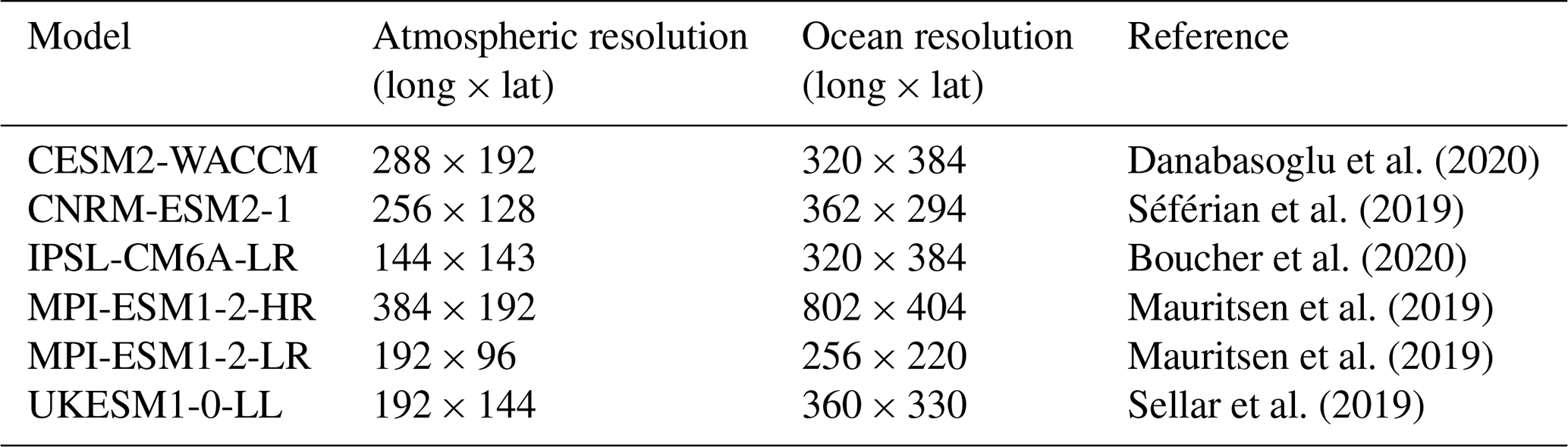
We used monthly data from the first realization in each scenario from all six earth system models (ESMs; Table 1) that have performed the CMIP6 and GeoMIP6 scenarios to estimate the ITF transport. The variable fields we use are the zonal and meridional wind stress (tauu and tauv), the seawater vertical velocity (wo), and the seawater salinity and temperature (so and thetao). All fields were bi-linearly interpolated (except for seawater vertical velocity, for which we use conservative interpolation) onto a common ${\mathrm{0.5}}^{\circ }\times {\mathrm{0.5}}^{\circ }$ grid.

Table 1 Earth system models (ESMs) used in this study.

3 Methods

3.1 Island Rule

In the Sverdrup balance, ocean current acceleration and friction are neglected and wind stress curl is the driving force of large-scale ocean circulation (Sverdrup, 1947). The “Island Rule” (Godfrey, 1989) uses the Sverdrup balance to calculate the net total flow through a region from the integral of the wind stress on a specific closed path. This is a simple and more efficient way of estimating the long-term magnitude and interannual variability than direct observations of flow through the complex channel topography of the Equator-spanning Indonesian archipelago (Godfrey, 1996). Feng et al. (2011) used an eddy-permitting numerical model, ORCA025, to verify that the Island Rule can capture the decadal variability of the ITF transport.

The original Island Rule assumes that the ocean is dormant below a moderate depth, Z, below which there is no motion (Sverdrup, 1947). The ITF transport is determined by the integral of the wind stress along the path that heads from the southern tip of Australia eastwards to South America, follows the coastline to the latitude line of the northwestern tip of Papua New Guinea (PNG), and then traces the west coast of Australia back to the starting point (Fig. 1a):

$$\begin{array}{}\text{(1)}& T_{\text{ITF}}={\displaystyle \frac{\mathrm{1}}{f_{\text{N}}-f_{\text{S}}}}\oint {\displaystyle \frac{{\mathit{\tau }}^{\text{l}}}{{\mathit{\rho }}_{\mathrm{0}}}}\mathrm{d}l,\end{array}$$

where f_N and f_S are the Coriolis parameters at the Equator and 44^∘ S, respectively. τ^l is the along-route wind stress component. ρ₀ is the mean seawater density.

3.2 Amended Island Rule

Studies have suggested that a decline in the ITF under GHG forcing was due to both the weakening of trade winds in the Pacific and the impact of the deep ocean circulation change (Feng et al., 2012; Hu et al., 2015). Sen Gupta et al. (2016) used a climate model to attribute the GHG-forced decrease in ITF transport to weakening of the deep Pacific upwelling. Feng et al. (2017) estimated the contribution of deep ocean upwelling from the Pacific north of 44^∘ S to produce the Amended Island Rule:

$$\begin{array}{}\text{(2)}& T_{\text{ITF}}={\displaystyle \frac{\mathrm{1}}{f_{\text{N}}-f_{\text{S}}}}\oint {\displaystyle \frac{{\mathit{\tau }}^l}{{\mathit{\rho }}_{\mathrm{0}}}}\mathrm{d}l+\int \underset{\text{Pacific}}{\int }{w}_z\mathrm{d}s,\end{array}$$

where w_z is the vertical velocity of the Pacific at 1500 m depth. The contribution of deep ocean upwelling is integrated over the whole Pacific north of 44^∘ S (considering volume conservation and that the sill depth of the Indonesian seas is less than 1500 m). The Amended Island Rule was verified with a near-global eddy-resolving ocean model simulation and found to estimate the interannual to decadal as well as the centennial variability of the ITF transport well (Feng et al., 2017). Here we describe the ITF using the Amended Island Rule and its component parts, which are the wind-driven Sverdrup balance, which we denote as wind, and the Pacific upwelling, which we denote as upwelling.

3.3 Buoyancy forcing

Sea levels in the Pacific and Indian oceans have been used to estimate the ITF transport in previous studies (Clarke and Liu, 1994; Potemra et al., 1997; Susanto and Song, 2015). Buoyancy accounts for the high steric sea level (that is, a volume increase due to a lower density) in the North Pacific (Stigebrandt, 1984). A pool of low-density water (the DBP) originating in the North Pacific is formed in the eastern Indian Ocean between the Indonesian islands and northwestern Australia (Fig. 1a). The sea level drop between the Indian and Pacific oceans occurs essentially at the abrupt eastern boundary of the DBP and is the source of buoyancy forcing (Andersson and Stigebrandt, 2005). In the DBP region, the long-term difference between the westward and eastward transport along the northern and southern flanks of the pool is the ITF transport.

The geostrophic transport in the DBP is related to denser water in the eastern Equatorial Indian Ocean (EIO):

$$\begin{array}{}\text{(3)}& {\displaystyle }{Q}_{\mathit{\lambda }}={\displaystyle \frac{g{H}^{\mathrm{2}}\mathrm{\Delta }\mathit{\rho }}{\mathrm{2}{f}_{\mathit{\lambda }}{\mathit{\rho }}_{\mathrm{0}}}}\text{(4)}& {\displaystyle }\text{ITF}=Q_{{\mathit{\lambda }}_{\text{N}}}-Q_{{\mathit{\lambda }}_{\text{S}}},\end{array}$$

where g is the acceleration due to gravity, H is the penetration depth of the DBP (set in Andersson and Stigebrandt, 2005 to 1200 m), f_λ is the Coriolis parameter at latitude λ, ρ₀ is the reference density at 1200 m, and the northern (λ_N) and southern (λ_S) boundary latitudes of the DBP are 10 and 16^∘ S, respectively. Δρ is the density difference between the DBP region (9–15^∘ S, 100–120^∘ E) and the EIO region (6^∘ N–6^∘ S, 80–100^∘ E). We denote the ITF given by Eq. (4) as “buoyancy”-driven ITF. Hu and Sprintall (2016) verified the use of DBP and EIO to calculate Δρ with observations.

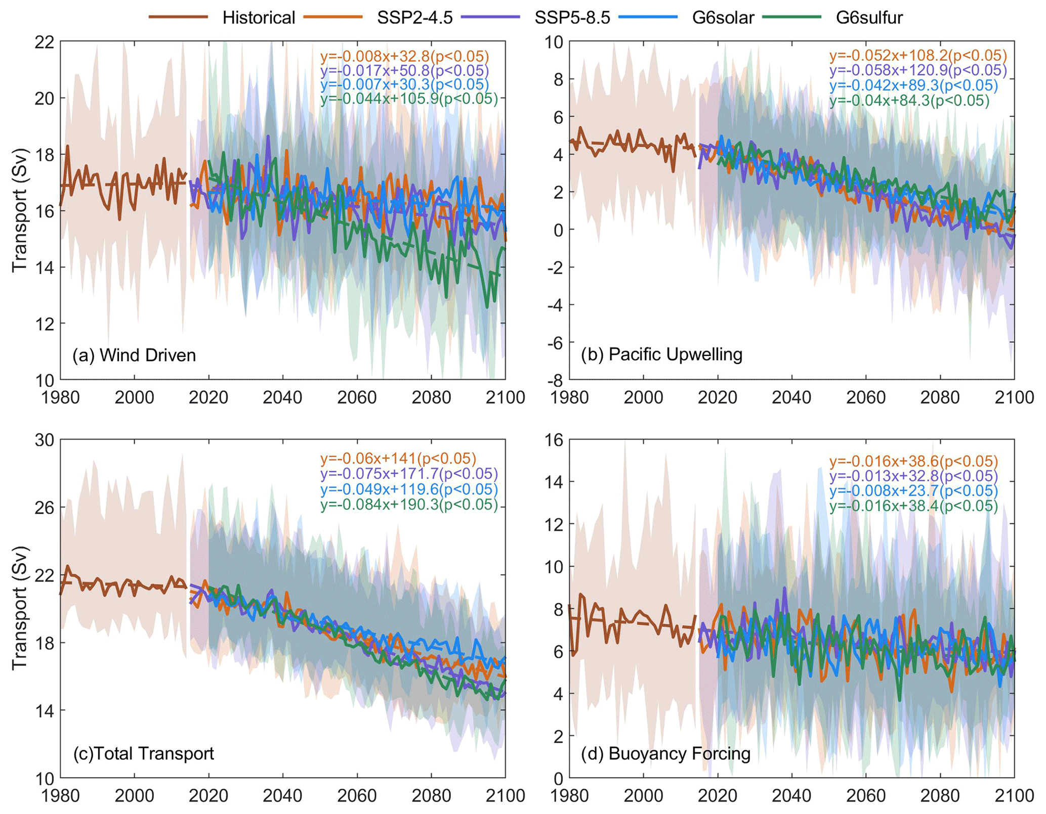
Figure 2 Six-ESM ensemble-mean ITF components under different scenarios. The shaded areas show the standard deviation and the equations are the regression trend lines (2015–2100 under the two SSP scenarios and 2020–2100 under the two G6 scenarios), each of which is followed by the significance of the slope. (a) Sverdrup balance wind-driven component. (b) Pacific upwelling north of 44^∘ S. (c) Wind + upwelling ITF under the Amended Island Rule (Eq. 2). (d) ITF transport by buoyancy forcing. Individual ESM results are shown in Fig. S1 in the Supplement.

4 Transport and geoengineering

4.1 ITF transport

The multi-model ensemble-mean wind-driven ITF transport is ∼16.9 Sv, with the Pacific upwelling north of 44^∘ S contributing ∼4.5 Sv, in the historical period (Fig. 2). This compares with observational estimates of about 15 Sv during 2004–2006 (Sprintall et al., 2009), and the multi-model ensemble mean (for a total of 22 CMIP5 models) is 15.2 Sv for 1900–2000 (Sen Gupta et al., 2016). Under SSP2-4.5 during 2015–2100, the wind-driven and Pacific upwelling contributions to ITF transport are not much different from those under SSP5-8.5. The wind-driven volume ITF transport shows significant trends for all scenarios, with the smallest trends seen for the SSP scenarios (linear trends of a lower magnitude than 0.02 Sv per year), while the upwelling contribution shows obvious downward trends in all scenarios. These trends appear to be consistent, despite differences in estimated transport across models (Fig. S1). Thus, the decline in future ITF transport in future GHG climates was explained by Feng et al. (2017) as being due to weakening of the Pacific upwelling on centennial timescales while wind-driven processes had no impact on long timescales.

During the last 20 years of the 21st century, the simulated ITF transport using the Amended Island Rule is 27 % ± 3 % (standard error) under SSP5-8.5 (Fig. 2c), with the Pacific upwelling decline accounting for 76 % ± 15 % (p<0.05, Wilcoxon signed rank test) of the wind + upwelling reduction. Both the wind-driven and upwelling contributions to ITF transport are slightly higher under SSP2-4.5 than under SSP5-8.5 during the same period, but the differences are small over the whole 2015–2100 period. The wind + upwelling ITF transport is reduced by 23 % ± 2 % (standard error, p<0.05) under SSP2-4.5 during the period of 2080–2100 relative to the historical period (cross ESM range 13 %–27 %), and the wind-driven component drops by only by 5 % (range −2 %–9 %). The reductions under SSP5-8.5 for the upwelling and wind-driven components are, respectively, 97 % (60 %–305 %) and 8 % (1 %–19 %).

Compared with the reasonable agreement for the Amended Island Rule estimates of ITF, the alternative buoyancy method behaves much worse. The simulated multi-mean ITF transport by buoyancy forcing is 7.3 Sv in the historical period, which is less than that produced by wind-driven processes and only half the transport observed during INSTANT (Sprintall et al., 2009), and there is large across-model variability (Fig. S2). Under the two SSP scenarios, the difference in ITF transport is small, with a significant trend occurring during 2015–2100. The buoyancy-driven estimation method can capture the interannual variability of ITF transport, but it does not perform well on centennial timescales (Hu and Sprintall, 2016), where the ITF is much closer to that from the wind-driven estimation method.

SAI and SD geoengineering methods clearly have different impacts on the wind-driven contributions to ITF transport for all models (Table S1) and the ensemble mean (Table 2) according to the Wilcoxon signed-rank test, and show smaller although still significant differences in upwelling for the six-model ensemble mean, although significant differences individually only for CESM2-WACCM (Fig. 2a, b, Tables 2, S1). Under the G6solar and G6sulfur scenarios, the wind + upwelling ITF transport is reduced by 19 % ± 1 % and 28 % ± 1 %, respectively, during 2080–2100 relative to the historical period, with the wind-driven ITF transport reduced by 4 % ± 1 % and 16 % ± 1 % and the upwelling transport volume reduced by 76 % ± 8 % and 70 % ± 10 %. All these differences between scenarios are significant (p<0.05, Wilcoxon signed-rank test; Table 2). Under G6sulfur, the wind-driven ITF transport shows a clear downward trend, in contrast with the other three climate scenarios (Fig. 2a). Each ESM also shows consistency in the relative declines under the four future climates (Fig. S1a). The decline in wind-driven transport accounts for 47 % (range 38 %–65 %) of the decline in wind + upwelling ITF transport under G6sulfur during 2080–2100, and its ensemble mean wind-driven transport volume is significantly lower than that under SSP5-8.5 (Table 2). The ensemble mean ITF transport by buoyancy forcing shows significant declining trends under all the future climate scenarios, but the differences are not generally significant (Fig. 2d, Table 2), which is different from the transport change calculated using the wind-driven and upwelling contributions.

Table 2 The differences in monthly ITF transport (2020–2100)^a and its components according to the different methods. “Wind” is the ITF transport derived from the Island Rule and used in the Amended Island Rule; “upwelling” is the area integral of the Pacific upwelling rate at 1500 m used in the Amended Island Rule; “wind + upwelling” is the ITF transport calculated by the Amended Island Rule; “buoyancy” is the ITF transport by buoyancy forcing and is used independently of the other two components. Unit: Sv (1 Sv = 10⁶ m³ s⁻¹).

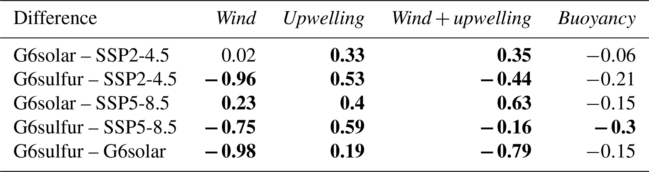
^a The end dates of G6solar and G6sulfur for MPI-ESM1-2-HR are 2099 and 2089, respectively, and those for MPI-ESM1-2-LR are both 2099. Values in bold are significant at the 95 % level according to the Wilcoxon signed-rank test.

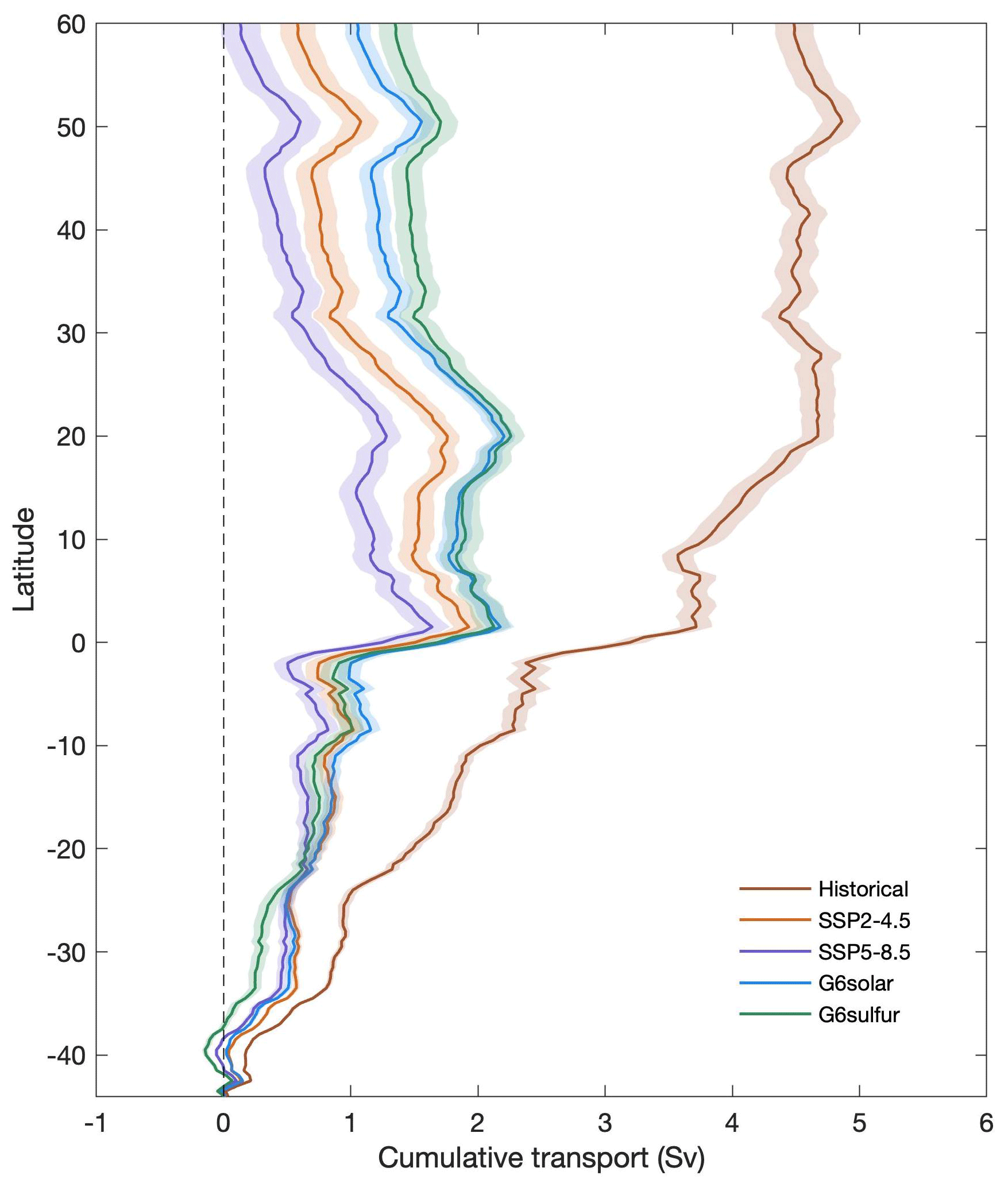
Figure 3 Multi-model ensemble-mean zonal cumulative transport by Pacific upwelling north of 44^∘ S during the historical simulation (1980–2014) and under the four future scenarios (2080–2100). Shaded areas show the standard error.

The decline in ITF transport via upwelling in the future relative to the present under each scenario is illustrated in Fig. 3. During the historical period, the zonally integrated (starting at 44^∘ S and proceeding northward until 60^∘ N) upwelling contributions to ITF transport in the Pacific Ocean steadily accumulate when progressing from southern latitudes until about 20^∘ N. Latitudes further north contribute little, so the accumulated upwelling is then fairly constant. This pattern changes in all future climate scenario simulations. The Pacific upwelling contributions to the transport volume accumulate steadily but slower with latitude than in the historical simulation up to just north of the Equator (2^∘ N), and then, after a small decrease, they rapidly accumulate over a few degrees of latitude. North of 20^∘ N, the integrated upwelling declines. Differences between scenarios in ocean upwelling velocity are not significant in the Pacific, except in the western boundary current region. Starting from 20^∘ N, the wind stress in the western boundary current region decreases and the upwelling of seawater weakens (Fig. 5), resulting in a reduced upwelling contribution in the future scenario. Between 44 and 15^∘ S, the zonal cumulative transport curves under SSP2-4.5 and G6solar are relatively similar. The integrated upwelling under the G6sulfur scenario transitions from being the smallest among the four future scenarios between 44 and 20^∘ S to being the largest a few degrees north of the Equator (Fig. 3).

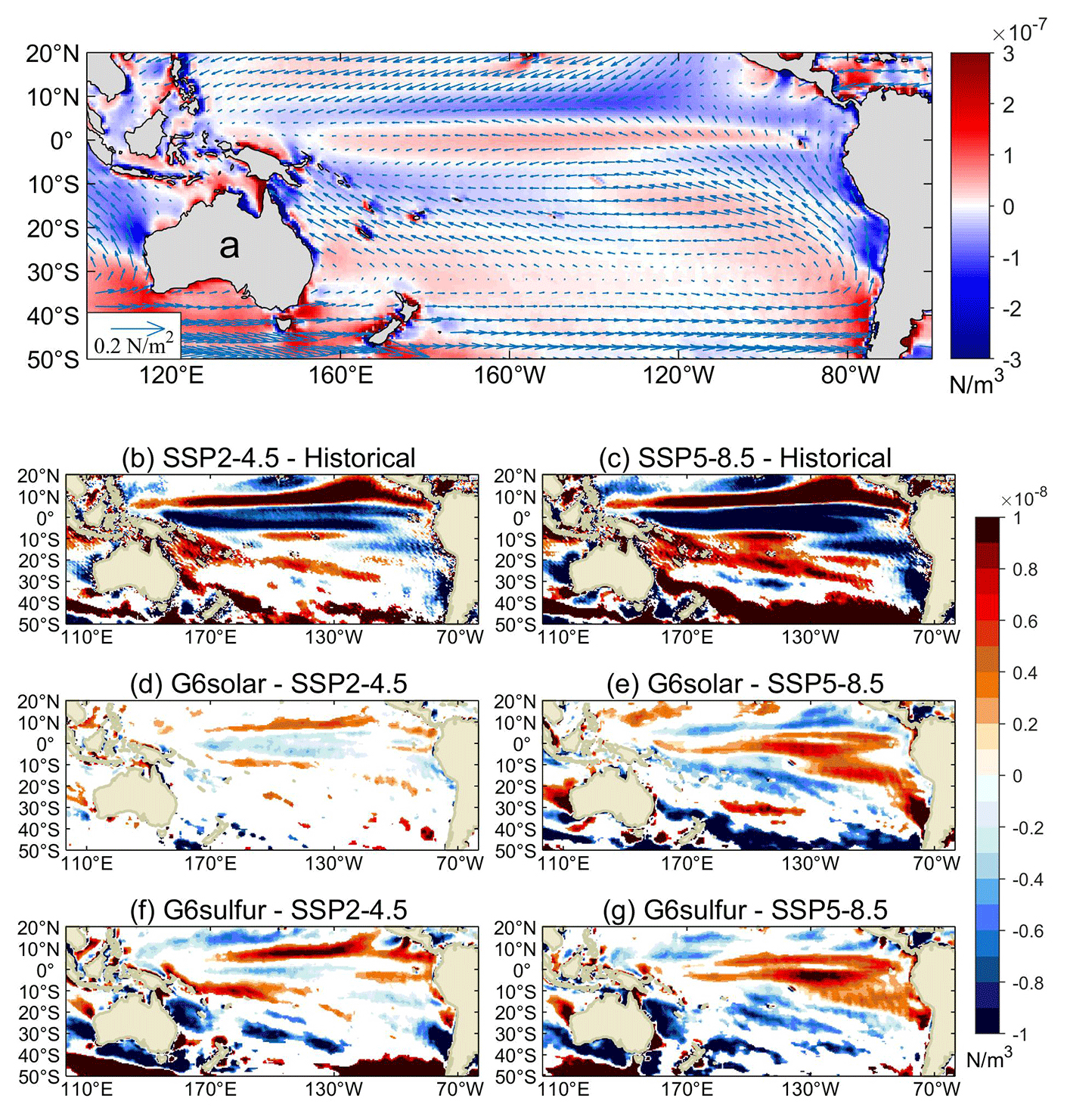
Figure 4 Multi-model mean differences in wind stress curl. (a) The historical mean; the arrows show the wind stress. Differences between (b) SSP2-4.5 and the historical period, (c) SSP5-8.5 and the historical period, (d) G6solar and SSP2-4.5, (e) G6solar and SSP5-8.5, (f) G6sulfur and SSP2-4.5, and (g) G6sulfur and SSP5-8.5. The historical period is 1980–2014 and the period for the future scenarios is 2080–2100. Regions where differences are not significant at the 95 % level according to the Wilcoxon signed-rank test are masked in white. Figure S3 shows the ITF inlet region around the Indonesian archipelago in more detail.

4.2 ITF by geoengineering type

4.2.1 Wind stress

Godfrey et al. (1993) suggested that the Indonesian Throughflow originates in the South Pacific, where the South Equatorial Current retroflects into the North Equatorial Countercurrent and enters the Indonesian Sea via the Mindanao Current. The wind stress curl is determined by the components of the wind stress vector and drives the ocean circulation (Gill and Adrian, 1982). Figure 4a shows the mean wind stress and the wind stress curl in the historical period (1980–2014); the wind stress curl is positive at low latitudes in the South Pacific, causing mass transport to the north. In the South Pacific, under the SSP2-4.5 scenario during 2080–2100, the wind stress curl in the middle latitudes is stronger than that in the historical period, while that at low latitudes and along the west coast of South America is weaker than in the historical period (Fig. 4a). The anomalies in the SSP5-8.5 scenario relative to the historical period are similar but extend over a larger region and have a larger amplitude (Fig. 4b). The net ITF transport volume under SSP5-8.5 is lower than that during the historical period, which is consistent with the difference in wind stress curl between the simulations. There is no significant difference in wind stress curl between G6solar and SSP2-4.5 in the mid-latitudes, and the difference in the low latitudes is relatively small (Fig. 4c). The wind stress curl under G6solar is slightly weaker at the mid-latitudes and slightly stronger at low latitudes than with SSP5-8.5 (Fig. 4d). Differences in wind stress curl between G6sulfur and SSP2-4.5 scenarios are mainly seen in the mid-latitudes, near the Equator and the west coast of South America (Fig. 4e), which are related to the wind-driven ITF transport changes. In contrast, the significant differences in wind stress curl between G6sulfur and SSP5-8.5 are mainly seen in the northeast of the South Pacific, and the wind stress curl under G6sulfur is stronger than that under SSP5-8.5 (Fig. 4f). The wind stress curl at the inlet of the ITF is significantly weakened under the G6sulfur scenario compared with the two SSP scenarios.

The multi-model average ITF transport shows significant differences between the G6 scenarios and the SSP scenarios during 2020–2100 (Table 2). Differences in wind-induced ITF transport from SSP2-4.5 are smallest with G6solar (Table 2) and are not significantly different in every ESM (Table S1). Differences between SSP5-8.5 and G6solar are the same sign for wind and upwelling forcings, contributing to larger differences in the Amended Island Rule wind + upwelling transport. With G6sulfur, wind and upwelling forcing differences from SSP5-8.5 have opposite signs, and the net transport difference is quite small but still significant for the six-model ensemble (Table 2). Differences in the ITF defined by buoyancy are only significant for G6sulfur–SSP5-8.5.

4.2.2 Upwelling

The spatial pattern of upwelling velocity at 1500 m in the Pacific under present day conditions has strong upwelling at the Equator, weak upwelling in the interior, and mixed up- and downwelling along the ocean boundaries (Feng et al., 2017). In future greenhouse gas climate scenarios, the main factor affecting ITF transport is net upwelling in the Pacific Ocean (Feng et al., 2017; Sen Gupta et al., 2016). Spatial patterns of upwelling changes are shown in Fig. 5.

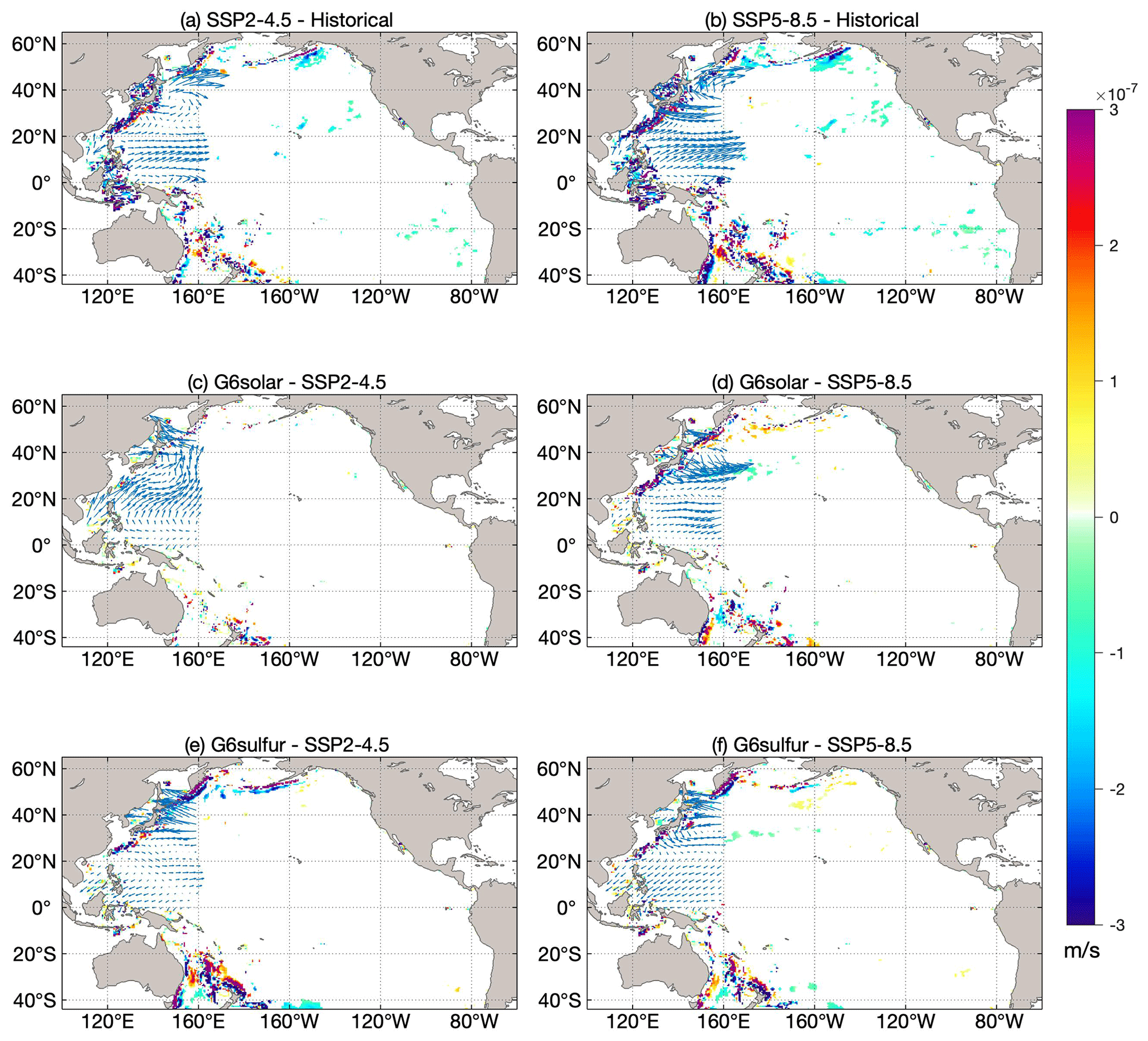
Figure 5 Changes in the multi-model ensemble-mean upwelling velocity at 1500 m (blue indicates increased upwelling; red indicates relative downwelling) and the wind stress differences (arrows) between (a) SSP2-4.5 and the historical period, (b) SSP5-8.5 and the historical period, (c) G6solar and SSP2-4.5, (d) G6solar and SSP5-8.5, (e) G6sulfur and SSP2-4.5, and (f) G6sulfur and SSP5-8.5. The historical period is 1980–2014 and the period for the future scenarios is 2080–2100. Regions where differences are not significant at the 95 % level according to the Wilcoxon signed rank test are masked in white.

Much of the ocean shows no significant change in upwelling velocity, but the western boundaries differ significantly from the historical period in both SSP scenarios (Fig. 5a, b), and under SSP5-8.5 there is also a significant upwelling in the equatorial eastern Pacific. The western boundary currents are an important source of ITF gradient differences in wind stress that drive ocean currents (Hu et al., 2015), and these gradients remain present at great depth in the western boundary current region.

The difference in upwelling velocity between the G6solar and SSP2-4.5 scenarios is insignificant almost everywhere (Fig. 5c), once again illustrating the similarities between the solar dimming experiment and its target SSP2-4.5 scenario. Differences from SSP5-8.5 are significant mainly along the extratropical western ocean boundaries. The outcome of the SAI experiment is clearly different from the solar dimming outcome. Differences between G6sulfur and the SSP scenarios are clearly larger than those between G6solar and the SSP scenarios and greater in the extratropics than in the tropics. The pattern of changes in upwelling anomalies for G6sulfur–SSP2-4.5 is similar but opposite in sign to that for G6solar–SSP5-8.5 (Fig. 5e), while the differences between G6sulfur and SSP5-8.5 are similar to or slightly smaller than differences between G6sulfur and SSP2-4.5 (Fig. 5f).

4.2.3 Seasonality

Seasonal patterns in ITF are important and reflect changes in the positions of the two main precipitation convergence zones across the region. Model simulations show that decreases in ITF transport in April–May and October–November and the recoveries following these decreases are due to the upper ocean changes associated with the Rossby waves in the Pacific Ocean, and they show that the seasonal ITF transport is closely related to wind variations in the Pacific and Indian oceans (Shinoda et al., 2012). The seasonal wind-driven ITF transport is at its maximum in June–August (JJA) and its minimum in December–February (DJF) under different scenarios (Fig. 6), which is consistent with the result in Wyrtki (1987). However, the differences between the G6 scenarios are largest in DJF and March–May (MAM), and these seasons are also when all four future scenarios are most different from the historical simulation.

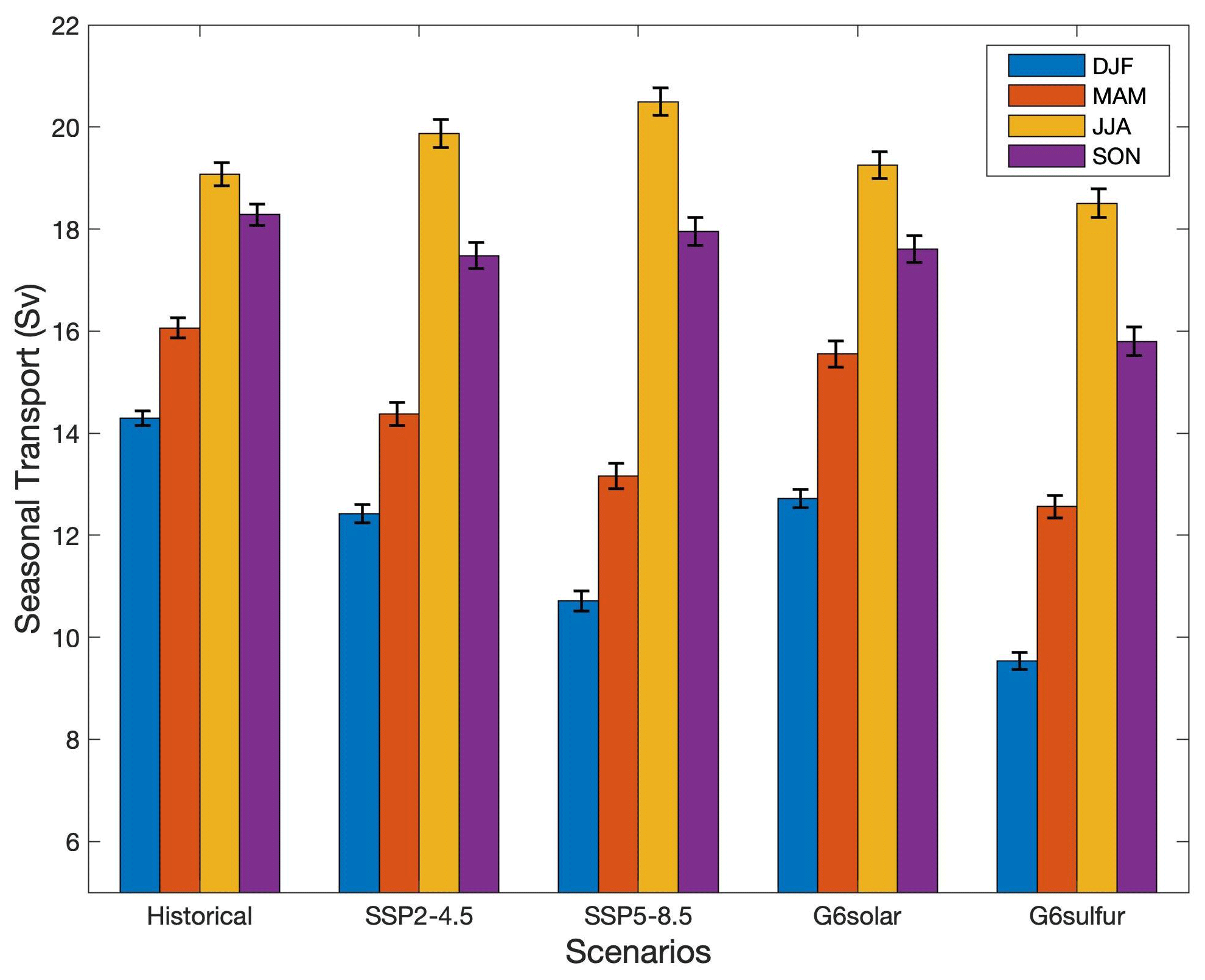
Figure 6 The ensemble-mean seasonal wind-driven ITF transport and the standard error during the historical period (1980–2014) and in future scenarios (2080–2100).

The South Pacific Convergence Zone (SPCZ) is a strong rainfall and convection zone extending from the Equator to the subtropical South Pacific which is generated by the low-level convergence between the northeast trade wind and weaker westerly wind (Vincent, 1994). The SPCZ is clearest in DJF, the Southern Hemisphere summer, and is marked in the top row of Fig. 7. The annual wind stress curl differences between G6solar and SSP2-4.5 are small, but the seasonal variation difference in some regions is significant. Under G6solar, compared with SSP2-4.5, the wind stress curl near the Equator is weakened in DJF. In MAM, the wind stress curl in the middle and low latitudes of the Southern Hemisphere is generally enhanced. SSP5-8.5 has significantly lower wind stress curl in the SPCZ region relative to G6solar in DJF. In MAM, they mainly differ in the mid-latitudes. From June through November (JJA and SON), the wind stress curl under SS5-8.5 is significantly lowered between 30 and 50^∘ S. In contrast, G6sulfur shows a significant increase in the SPCZ region in DJF and a significant decrease south of the SPCZ region in JJA relative to SSP2-4.5. There are large differences in the ocean northeast of New Zealand, with the sign reversing from MAM to JJA. The differences between G6sulfur and SSP5-8.5 are not very much bigger than the differences between G6sulfur and SSP2-4.5, and the patterns are quite similar. The wind stress curl in the SPCZ region and its extension southeastwards is significantly weakened under G6sulfur relative to both SSP scenarios in DJF. In JJA, the region with a decrease in wind stress curl east from New Zealand is slightly larger relative to SSP5-8.5 and SSP2-4.5.

4.3 ITF and ENSO

The wind-driven ITF transport estimated using the six CMIP6 models for the historical scenario is well within the range of 11–20 Sv found from 22 CMIP5 models (Sen Gupta et al., 2016). These model estimates tend to slightly overestimate the ITF compared with the observed ITF (15 ± 3 Sv) since Godfrey's Island Rule ignores the friction due to the real ocean topography (Feng et al., 2005; Wajsowicz, 1993). The rather large interannual and decadal variations in the ITF (amounting to several Sv) are mainly influenced by the Pacific and Indian ocean winds. There is an observed relationship between ITF transport and the El Niño–Southern Oscillation (ENSO), with stronger transport seen during La Niña and weaker transport seen during El Niño and with the ITF variability lagging the ENSO variability by 8–9 months (England and Huang, 2005; Meyers, 1996).

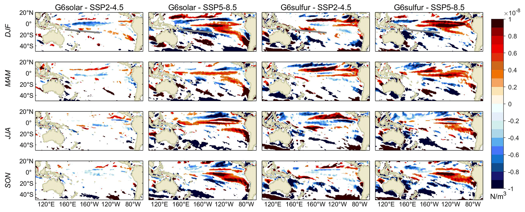
Figure 7 Seasonal ESM ensemble-mean spatial differences (G6solar – SSP2-4.5, G6solar – SSP5-8.5, G6sulfur – SSP2-4.5, and G6sulfur – SSP5-8.5) in the wind stress curl during 2080–2100. The gray lines in each panel in the top row mark the mean position of the South Pacific Convergence Zone (SPCZ) in DJF based on the CMIP6 multi-model mean (Brown et al., 2020). Regions where differences are not significant at the 95 % level according to the Wilcoxon signed rank test are masked in white; significant differences are larger than $|\mathrm{0.5}\times {\mathrm{10}}^{-\mathrm{8}}|$ Nm⁻³.

We seek relationships between ITF and ENSO variability using a wavelet coherence analysis (Grinsted et al., 2004) of Nino3.4 and the wind-driven ITF anomaly. This method examines the correlations and phase between two time series and is useful for exploring potential causality relationships (e.g., Grinsted et al., 2004; Xia et al., 2023). Since the models are not adjusted to match observations, the natural variability in the oceans is not synchronized, and so a multi-model ensemble will not show useful phase relationships. Therefore, we instead show just the CESM2-WACCM model in Fig. 8, while the other models are shown in Fig. S4. Figures 8 and S4 show an obvious annual coherence for all models, as could be expected given that both time series have clear seasonality, but this is not actually significant with respect to the phase-randomized Fourier background hypothesis. There are significant multi-year coherence episodes in all models, though there are no significant differences in coherence between the scenarios at any band between annual and decadal. The two appear to be in antiphase (Fig. 8), in line with the observed stronger transport during La Niña and the weaker transport during El Niña. At the same time, ITF variability also lags behind ENSO on the whole, but there are differences among different models.

5 Summary and discussion

The six ESMs we use concur in the weakening of ITF transport in all future scenarios. That is, SRM cannot restore the ITF to its historic levels (Table 2, Fig. 2). This contrasts somewhat with the changes simulated in the AMOC under SRM with GHG forcing, where it seems that SRM can partly reverse the slowdown of the AMOC induced by GHG forcing, reducing its impact from around 35 % to 24 % (Muri et al., 2018; Tilmes et al., 2020; Xie et al., 2022). This illustrates the important regional variability in responses to SRM.

Weakening of the ITF transport appears in all future scenarios whether they have pure GHG forcing or combine GHG and SRM strategies. The ITF transport changes are defined almost totally (around 90 %) by significant differences in Pacific upwelling (Fig. 2a, b). This is consistent with the conclusion that the weakening trend in the ITF under global warming predicted by high-precision ocean models is not directly related to the change in Pacific trade winds but to the reduction in Pacific deep-sea upwelling (Feng et al., 2017). On centennial scales, the decrease in the net deep ocean upwelling in the tropics and the South Pacific (especially the changes in the western boundary current system) is what determines ITF transport. Buoyancy forcing can only estimate the interannual variation in the ITF, and our study supports the utility of the Amended Island Rule in estimating centennial changes in ITF transport. The Island Rule was specifically formulated considering the difficulties involved in measuring the flow in a complex topography. Instead, the Sverdrup theory of wind forcing was utilized, allowing much larger scale observations to provide useful estimates of the ITF. This methodology should also be suitable for the global models we have analyzed here. This contrasts with the relatively small region of the DBP (Fig. 1) that may not be consistently captured in the global models we analyze.

Sen Gupta et al. (2021) note that the projected weakening of the ITF and the differences between ESMs can be explained by changes in large-scale surface winds. This contrasts with our findings, where changes in wind-driven transport are not significantly different between models; instead, upwelling in the extratropical western boundary zones dominates the changes between scenarios. However, the western boundary currents are deep and narrow and differ from the shallow and wide eastern boundary currents. The tropics experience weaker (and reversed) trade winds compared to those that dominate the extratropical regions. The geographical differences in upwelling suggest that wind changes are driving the overall changes in ITF via upwelling regions, in effect supporting the conclusion of Sen Gupta et al. (2021) that differences in future surface winds explain most of the differences in future large-scale current systems.

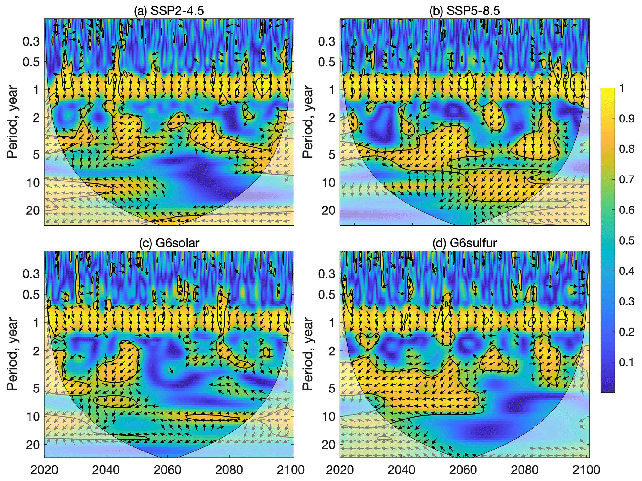
Figure 8 The squared wavelet coherence between the Nino3.4 (representing the ENSO) and the wind-driven ITF transport monthly anomalies under the two SSPs (2015–2100) and the two G6 scenarios (2020–2100) in the CESM2-WACCM model. The 95 % significance level from a Monte Carlo-generated 1000-member ensemble of series of identical mean and standard deviation with identical power spectra but phase-randomized Fourier noise (chosen instead of the usual first-order autoregressive null hypothesis here because of the strong annual signal; Xia et al., 2023) is represented by a thick contour line. The arrows indicate the relative phase relationship; that is, in-phase points to the right, antiphase points to the left, an up arrow indicates that the ITF anomaly leads the ENSO by 90^∘, and a down arrow indicates that the ITF anomaly lags the ENSO by 90^∘. The other models are shown in Fig. S4.

SSP2-4.5 global radiative forcing was the design target of the G6 experiments despite GHG concentrations being at SSP5-8.5 levels. The difference in wind stress curl between G6solar and SSP2-4.5 indicates that the SD experiment performs better at reversing GHG-induced changes in Pacific wind than G6sulfur. The G6sulfur SAI experiment leads to a significant change in the winds in the mid- and low-latitude Pacific Ocean, which results in even lower estimated ITF transport than under the high GHG SSP5-8.5 forcing alone. Furthermore, G6sulfur also impacts deep ocean upwelling, especially in the extratropical western boundary current region, such that the ITF transport during the 21st century under the G6sulfur scenario is slower than that under the G6solar scenario. The G6 scenarios do not affect low-latitude western boundary currents and upwelling; for example, the upwelling near the Mindanao Current is unaffected, while the upwelling along the Kuroshio Current is apparently displaced in both G6 experiments. The ITF transport under the SD experiment was stronger than that under the SAI experiment and even higher than its target SSP2-4.5 scenario level at the end of the 21st century.

Changes in circulation in the future will have important impacts on aquatic ecology and fisheries (Dubois et al., 2016). In fact, the populations in Indonesia's coastal areas, especially those in the islands through which the ITF passes, are highly dependent on fisheries, and hence the changes in ITF under both pure GHG and mixed GHG and SRM scenarios will have important local implications for the livelihoods and ways of life of the local populations. Seasonal variations in ITF transport reflect important processes in the tropical convergence zones, and these are clearly impacted by all four future scenarios in generally subtle ways. But the largest differences are seen between the two most challenging scenarios to simulate – SSP5-8.5 and G6sulfur. Despite the large size of the perturbation that these forcings apply in the simulations, and the differences between climate models in parameterizing the SAI schemes, the findings are rather robust in terms of the changes to the winds in all seasons in the Pacific Ocean and Maritime Continent.

SAI is a far more feasible method of SRM than SD (Shepherd, 2009), but it produces far larger differences in various climate fields from GHG and historic simulations than SD does (Visioni et al., 2021), and far larger across-ESM differences, as the models process the aerosol impacts in varied ways (Visioni et al., 2021). The differences in winds noted in G6sulfur likely arise from differences in stratospheric heating due to the sulfur aerosols, which then drive tropospheric circulation changes (Visioni et al., 2020).

Although ESMs can provide reliable predictions of the ITF transport, the accuracy of global meso- and small-scale spatial and seasonal changes remains an issue. These relatively small-scale differences are potentially more important for local impacts than differences in larger-scale or annual changes. These aspects will need to be explored using impact models tailored to the region – ideally through initiatives focused on the Global South like the Degrees Initiative (https://www.degrees.ngo/, last access: 5 December 2023) and addressing concerns raised by local rightsholders.