Synchronization phenomena observed in glacial–interglacial cycles simulated in an Earth system model of intermediate complexity

The glacial–interglacial cycles of the Quaternary exhibit 41 kyr periodicity before the Mid-Pleistocene Transition (MPT) around 1.2–0.8 Myr ago and ∼ 100 kyr periodicity after that. From the viewpoint of dynamical systems, proposed mechanisms generating these periodicities are broadly divided into two types: (i) nonlinear forced responses of a mono- or multi-stable climate system to the astronomical forcing or (ii) synchronization of internal self-sustained oscillations to the astronomical forcing. In this study, we investigate the dynamics of glacial cycles simulated by the Earth system model of intermediate complexity CLIMBER-2 with a fully interactive carbon cycle, which reproduces the MPT under gradual changes in volcanic-CO₂ degassing and regolith cover. We report that, in this model, the dominant frequency of glacial cycles is set in line with the principle of synchronization. It is found that the model exhibits self-sustained oscillations in the absence of astronomical forcing. Before the MPT, glacial cycles synchronize to the 41 kyr obliquity cycles because the self-sustained oscillations have periodicity relatively close to 41 kyr. After the MPT the timescale of internal oscillations becomes too long to follow every 41 kyr obliquity cycle, and the oscillations synchronize to the 100 kyr eccentricity cycles that modulate the amplitude of climatic precession. The latter synchronization occurs with the help of the 41 kyr obliquity forcing, which enables some terminations and glaciations to occur robustly at their right timing. We term this phenomenon vibration-enhanced synchronization because of its similarity to the noise-enhanced synchronization known in nonlinear science. While we interpret the dominant periodicities of glacial cycles as the result of synchronization of internal self-sustained oscillations to the astronomical forcing, the Quaternary glacial cycles show facets of both synchronization and forced response.

1 Introduction

Glacial–interglacial cycles are pronounced climatic oscillations accompanied by massive changes in the global ice volume (Rohling et al., 2014; Spratt and Lisiecki, 2016), greenhouse gas concentrations (Bereiter et al., 2015; Lüthi et al., 2008; Petit et al., 1999) and temperatures (Jouzel et al., 2007; Snyder, 2016). Changes in global ice volume are recorded, e.g., in the oxygen isotope ratio δ¹⁸O of benthic foraminifera in marine sediments (Lisiecki and Raymo, 2005) (Fig. 1d, black), where higher δ¹⁸O values indicate larger ice volumes and cooler deep-ocean temperatures. The glacial cycles have relatively small-amplitude oscillations with dominant 41 kyr periodicity until ∼ 1.2–0.8 million years before present (Myr BP), while during the more recent part of the Pleistocene, they are characterized by larger amplitudes and a dominant periodicity of ∼ 100 kyr (black in Fig. 1h and i). This transition is called the Mid-Pleistocene Transition (MPT).

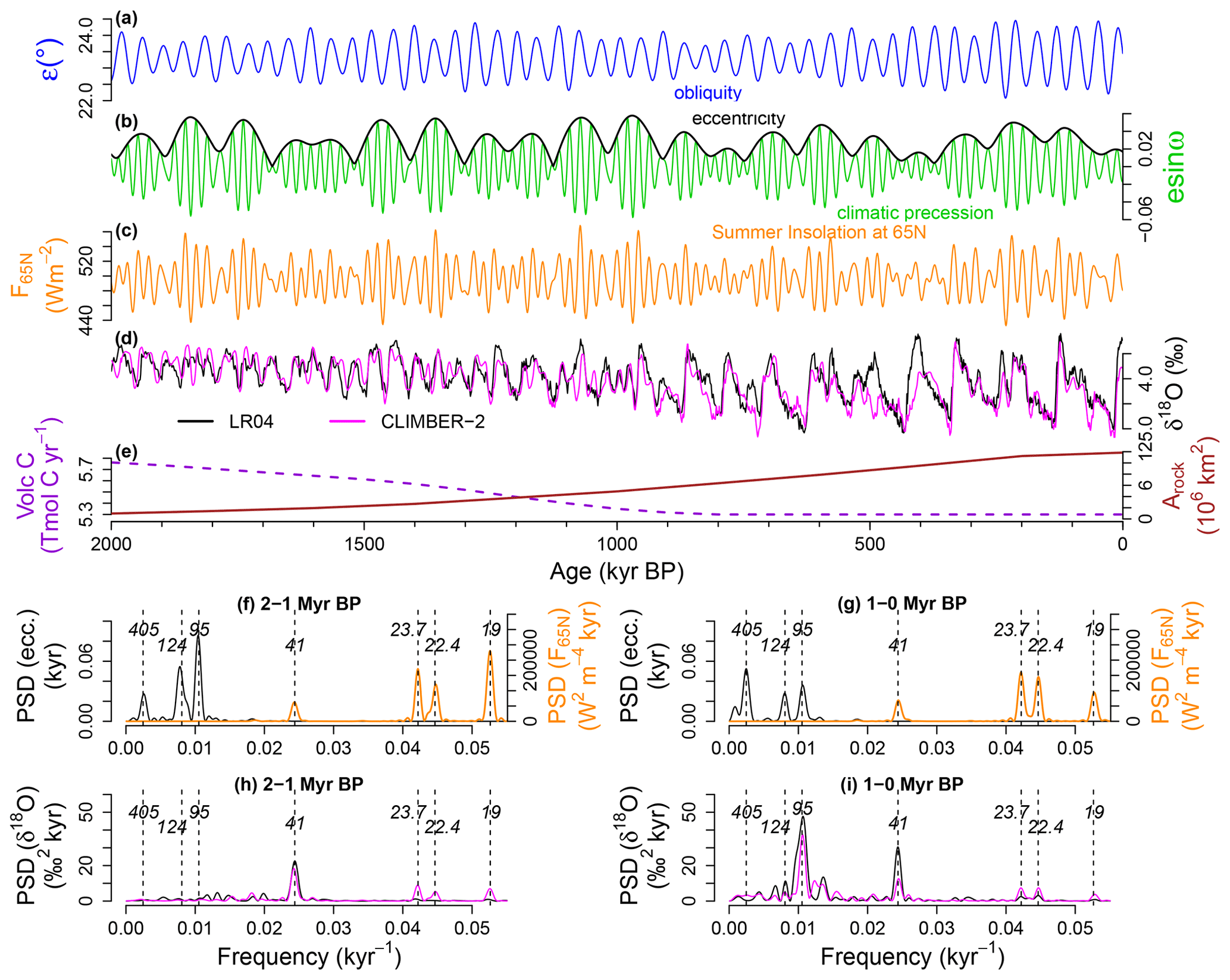
Figure 1 Time series and power spectral densities (PSDs) of the astronomical forcing (Laskar et al., 2004) and glacial cycles over the last 1 Myr. (a) Obliquity (blue). (b) Climatic precession (green) and eccentricity (black). (c) Boreal summer solstice insolation at 65^∘ N. (d) LR04 δ¹⁸O stack (Lisiecki and Raymo, 2005) (black) representing glacial–interglacial cycles during the last 2 Myr and corresponding CLIMBER-2 δ¹⁸O simulation by Willeit et al. (2019a) (magenta) under the optimal background condition scenario shown in (e). Note that the vertical axis is reversed so that larger δ¹⁸O values, corresponding to colder conditions, are lower. (e) Optimal scenario (Willeit et al., 2019a) for the volcanic-CO₂ (Volc C) outgassing rate (violet, dashed) and the area of exposed crystalline bedrock, A_rock (red, solid). (f) PSD of the eccentricity (black) and the PSD of the summer solstice insolation F_65N (orange) over the interval from 2 to 1 Myr before present (BP). (g) Same as (f) but over the interval from 1 Myr to present. (h) PSD of the LR04 δ¹⁸O record (black) and PSD of the optimal CLIMBER-2 simulation (magenta) over the 2 Myr-to-1 Myr interval. (i) Same as (h) but over the 1 Myr-to-present interval. The dashed vertical lines in (f)–(i) indicate major astronomical periodicities (Laskar et al., 2004).

There is general agreement that the glacial cycles are in some way paced by changes in the incoming solar radiation (i.e., insolation) caused by long-term variations in astronomical parameters (Hays et al., 1976): (i) the obliquity ε (Fig. 1a) describes the Earth's axial tilt and has a dominant periodicity around 41 kyr; (ii) the eccentricity e of the orbit (Fig. 1b, black) has dominant periodicities at 95, 124 and 405 kyr; and (iii) the climatic precession esin ω (Fig. 1b, green), with dominant periodicities at 23.7, 22.4 and 19 (18.95) kyr, varies with the longitude of the perihelion relative to the moving spring equinox ω, and its amplitude is modulated by the eccentricity, as shown in Fig. 1b (Laskar et al., 2004). The dominant frequencies of climatic precession are mechanically related to those of the eccentricity: $\mathrm{1}/\mathrm{19}-\mathrm{1}/\mathrm{23.7}\simeq \mathrm{1}/\mathrm{95}$, $\mathrm{1}/\mathrm{19}-\mathrm{1}/\mathrm{22.4}\simeq \mathrm{1}/\mathrm{124}$, and $\mathrm{1}/\mathrm{22.4}-\mathrm{1}/\mathrm{23.7}\simeq \mathrm{1}/\mathrm{405}$ kyr⁻¹ (Berger et al., 2005).

Milankovitch (1941) proposes that the glacial cycles are caused by summer insolation changes at high northern latitudes (Fig. 1c), where ice sheets can widely expand. Boreal summer insolation has prominent periodicities on the 19–23.7 kyr climatic precession band and on the 41 kyr obliquity band, while it has negligible power near the 100 kyr band (Fig. 1f and g, orange). Nevertheless, the dominant periodicity of glacial cycles is ∼ 100 kyr over the last 1 Myr (Fig. 1i, black): the 100 kyr problem (Imbrie et al., 1993; Paillard, 2001; Lisiecki, 2010). The climate system must thus exhibit some mechanism which produces the ∼ 100 kyr periodicity, although the input powers concentrate in the ∼ 20 and 41 kyr bands.

Previous studies link the ∼ 100 kyr glacial cycles with two or three obliquity cycles (Huybers and Wunsch, 2005; Bintanja and Van de Wal, 2008), four or five climatic precession cycles (Raymo, 1997; Ridgwell et al., 1999; Cheng et al., 2016), eccentricity cycles (Lisiecki, 2010; Rial, 1999), or combinations thereof (Tziperman et al., 2006; Huybers, 2011; Ganopolski and Calov, 2011; Parrenin and Paillard, 2012; Abe-Ouchi et al., 2013; Tzedakis et al., 2017). Upon closer look, the ∼ 100 kyr peak in Fig. 1i is located near the 95 kyr periodicity where the eccentricity has a spectral peak (Fig. 1g, black), suggesting a possible influence of the eccentricity cycle on the glacial cycles (Rial, 1999). On the other hand, the strongest periodicity of the eccentricity, at 405 kyr over the last 1 Myr, is hardly apparent in the power spectral density (PSD) of the glacial cycles (Fig. 1i): the 400 kyr problem (Imbrie and Imbrie, 1980). Hence, the mechanism producing the 100 kyr periodicity would additionally have to involve a damping of the 405 kyr eccentricity periodicity. Another mystery is the dominant 41 kyr periodicity before the MPT, which corresponds to the period of obliquity cycles. While several mechanisms have been proposed for the strong 41 kyr power (Raymo and Nisancioglu, 2003; Raymo et al., 2006; Huybers, 2006), recent results reveal influences of precession cycles in the temporal patterns of pre-MPT glacial cycles (Liautaud et al., 2020; Barker et al., 2022; Watanabe et al., 2023).

From the viewpoint of dynamical systems, the various proposed mechanisms to explain glacial cycles can be broadly classified into two types: synchronization and nonlinear response. Synchronization is the phenomena of frequency entrainment and phase-locking of oscillators, coupled uni- or bidirectionally (Pikovsky et al., 2003). Synchronization is a rather ubiquitous phenomenon in nature; a familiar example is the synchronization of human circadian rhythms to 24 h external day–night cycle. Synchronization requires internal self-sustained oscillations in the absence of external forcing, which are going to be synchronized to the external forcing (Pikovsky et al., 2003). When glacial cycles synchronize to the astronomical forcing, the frequency of glacial cycles is entrained at one of the astronomical frequencies, a subharmonic, or a combination tone thereof (see Appendix A). Phase or frequency lockings of self-sustained oscillations to one over two to three obliquity cycles or to one over four to five precession cycles are examples of subharmonic synchronization leading to ∼ 100 kyr glacial cycles. In synchronization theory, the external forcing is commonly assumed to be comparably weak so that the internal self-sustained oscillations are not drastically altered by the forcing (Pikovsky et al., 2003). Even if the forcing is weak, synchronization can generally occur if the frequency of internal oscillations is close to the frequency of the external forcing – the principle of synchronization. Therefore, if the glacial cycles with a dominant periodicity are generated consistently with the synchronization mechanism, the system is expected to exhibit unforced oscillations of a similar timescale. A number of models and theories describe the glacial cycles using the notion of synchronization (Saltzman et al., 1984; Gildor and Tziperman, 2000; Ashkenazy and Tziperman, 2004; Lisiecki, 2010; De Saedeleer et al., 2013; Crucifix, 2013; Ashwin and Ditlevsen, 2015; Mitsui et al., 2015; Nyman and Ditlevsen, 2019).

On the other hand, nonlinear response mechanisms attempt to explain the ∼ 100 kyr cycles without assuming underlying self-sustained oscillations, which include several proposed threshold mechanisms (Raymo, 1997; Paillard, 1998; Abe-Ouchi et al., 2013; Tzedakis et al., 2017) as well as various types of resonance or amplification of the forcing (Hagelberg et al., 1991; Le Treut and Ghil, 1983; Rial, 1999; Daruka and Ditlevsen, 2016; Verbitsky et al., 2018; Benzi et al., 1982; Nicolis, 1981). In general, synchronization and nonlinear response are distinguished with respect to the existence of internal self-sustained oscillations. However, as revisited in Sect. 5 below, their distinction can be subtle and practically very difficult if the external forcing is comparatively large or if noise-induced oscillations, which arise in excitable systems, are “synchronized” to a periodic forcing (i.e., stochastic resonance) (Pikovsky et al., 2003).

In this study we report self-sustained oscillations and their synchronization to the astronomical forcing in glacial cycles simulated in the Earth system model of intermediate complexity (EMIC) CLIMBER-2 with a fully interactive carbon cycle, specifically the version by Willeit et al. (2019a). The finding of self-sustained oscillations at the timescales of glacial cycles is not new in simple models but new in comprehensive EMICs. It has been previously shown that CLIMBER-2 can reproduce the characteristics of Quaternary glacial cycles including the MPT using slowly changing volcanic-CO₂ outgassing and regolith cover (Willeit et al., 2019a). So far various explanations have been proposed for the MPT such as a nonlinear ice sheet response to a long-term cooling trend (Berger et al., 1999; Bintanja and Van de Wal, 2008) possibly due to a long-term decline in the atmospheric CO₂ concentration, an onset of a positive feedback between the glacial intensification and additional glacial CO₂ drawdown by dust-borne iron fertilization (Chalk et al., 2017), an activation of the sea ice switch mechanism (Gildor and Tziperman, 2000), a change in the East Antarctic ice sheet margin from land-based to marine-based (Raymo et al., 2006), and the gradual removal of regolith by glacial erosion and an exposure of high-friction crystalline bedrock (Clark and Pollard, 1998). On the other hand, some models capture the frequency change across the MPT without any changes in their internal parameters, suggesting that the MPT is caused, at least in part, by changes in the astronomical parameters (Imbrie et al., 2011; Watanabe et al., 2023). Thus the physical mechanism of the MPT is still actively debated (Berends et al., 2021; Ford and Chalk, 2020; Clark et al., 2021; Legrain et al., 2023). The purpose of this study is not to re-examine the physical mechanisms leading to the MPT in CLIMBER-2, which is discussed in Willeit et al. (2019a), but to show novel synchronization phenomena underlying the glacial cycles simulated in the model.

The remainder of this article is organized as follows. Section 2 describes the data and the model setting. In Sect. 3, we show that CLIMBER-2 exhibits spontaneous oscillations in the absence of the astronomical forcing, supporting the view of synchronization; the lengthening of the timescale of internal oscillations leads to the change in the entrained frequency across the MPT. In Sect. 4, we show that the frequency entrainment at the ∼ 100 kyr power is achieved by cooperative action of climatic precession and obliquity forcing, via a novel nonlinear mechanism, which we term vibration-enhanced synchronization. Section 5 is devoted to summary and discussion.

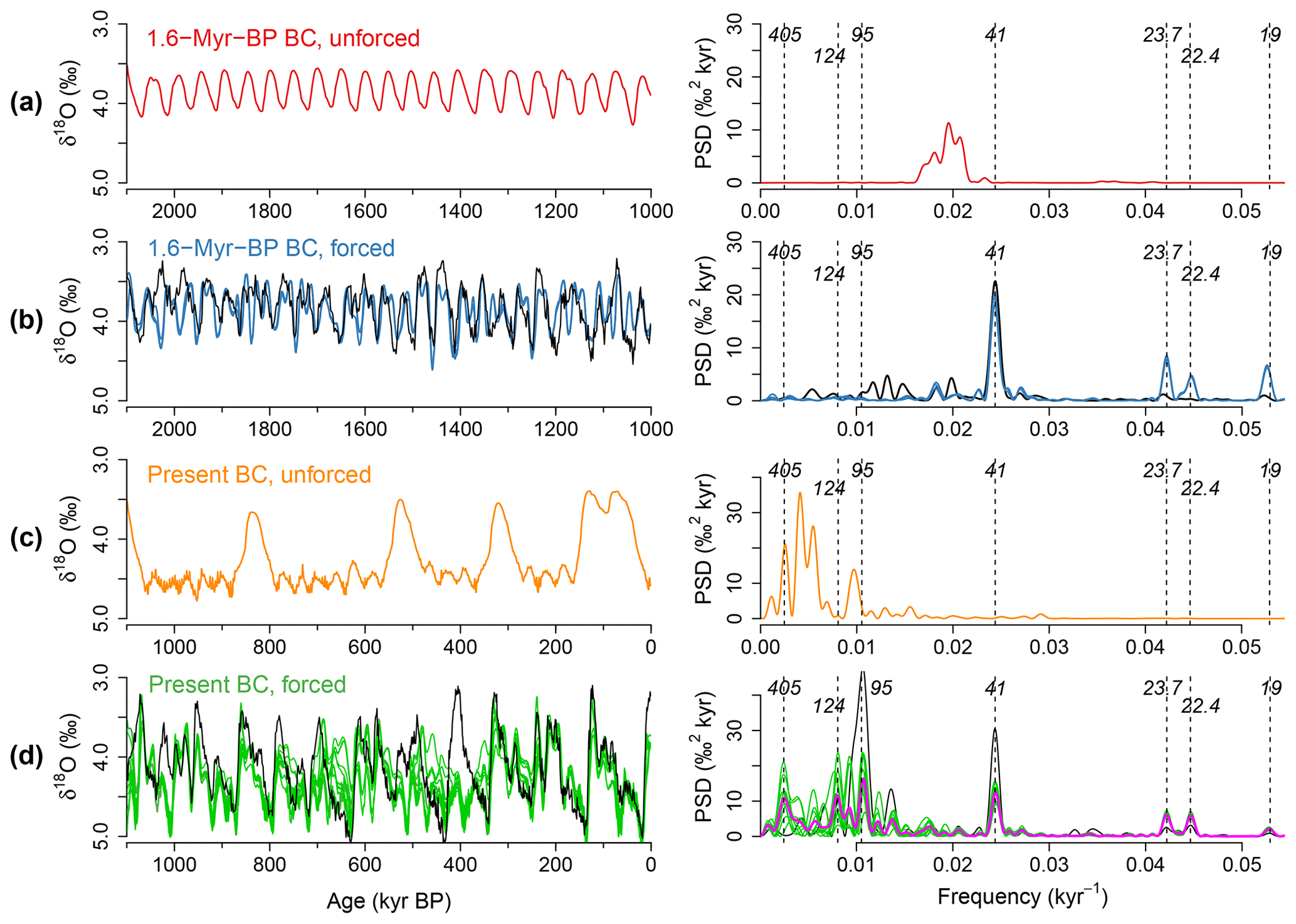
Figure 2 Comparison between unforced and forced simulations. (a) Unforced simulation of δ¹⁸O under 1.6 Myr BP background conditions (BC) and fixed orbital configuration with zero eccentricity and mean obliquity (left). The corresponding power spectral density (PSD) over 2–1 Myr BP (right). (b) Same as (a) but for true astronomical forcing (blue). The results for three slightly different initial times (i.e., initial orbital configurations) are shown. The black line corresponds to the δ¹⁸O record (Lisiecki and Raymo, 2005). (c) Unforced simulations under 0 Myr BP BC and fixed orbital configuration with zero eccentricity and mean obliquity. (d) Same as (c) but for true astronomical forcing (green). The results for 10 slightly different initial times (i.e., initial orbital configurations) are shown. The magenta line in the right panel is the ensemble average of the 10 PSDs. The black line corresponds to the δ¹⁸O record.

2 Methods

2.1 δ¹⁸O record

The benthic δ¹⁸O stack record (LR04) (Lisiecki and Raymo, 2005) is used throughout this study as empirical ground truth. It should be noted that the frequency and the strength of each spectral peak can in principle be affected by the orbital tuning of the record; a conservative tuning strategy is taken for the LR04 δ¹⁸O record. Investigating the chronology of the record is however beyond the scope of this work. We assume that the frequency structure of the LR04 record is basically correct including the observed dominance of 95 kyr periodicity over the last 1 Myr (Fig. 1i). The 95 kyr spectral peak is indeed observed in both orbitally tuned and untuned δ¹⁸O records, although it is slightly subdued in untuned records (Rial, 1999). The conclusions are derived from model simulations that are not subject to possible circular reasoning due to the orbital tuning.

2.2 CLIMBER-2 model and setting

Our study is based on an Earth system model of intermediate complexity (EMIC) called CLIMBER-2 (Petoukhov et al., 2000; Ganopolski et al., 2001, 2010; Ganopolski and Calov, 2011; Brovkin et al., 2012; Ganopolski and Brovkin, 2017; Willeit et al., 2019a). It couples atmosphere, ocean, vegetation, global carbon and dust models and a three-dimensional thermomechanical ice sheet model (Greve, 1997). This is the most comprehensive EMIC that, thanks to its exceptional simulation speed, still allows the analysis required here to be performed, with a large number of million-year-scale simulations. The glaciogenic dust is one of the key feedback mechanisms in CLIMBER-2 (Ganopolski et al., 2010; Ganopolski and Calov, 2011). It is assumed to be sourced from the terrestrial sediments exported from the margins of ice sheets. Its deposition reduces ice albedo and enhances ablation. In CLIMBER-2, some glacial terminations are only possible with the glaciogenic dust feedback (Ganopolski et al., 2010; Ganopolski and Calov, 2011). The importance of the dust loading for complete terminations has also been proposed earlier by Peltier and Marshall (1995). The CLIMBER-2 version used in this study is the same as used by Willeit et al. (2019a), which is slightly different from the earlier version used by Ganopolski and Brovkin (2017) with respect to the dust cycle scheme, the permafrost model and the regolith mask. Although the differences between these versions appear to be small, the underlying dynamics in the absence of forcing are different. We come back to this point in the discussion.

Willeit et al. (2019a) simulated the glacial cycles over the last 3 Myr, assuming scenarios about a long-term reduction in the volcanic-CO₂ outgassing rate and gradual changes in ice sheet substratum from regolith to hard-friction crystalline bedrock by glacial erosion (Fig. 1e), which we call the background condition (BC). Older BCs are characterized by a higher volcanic-CO₂ outgassing rate and wider area of regolith (the continents are assumed to be fully covered by regolith at 3 Myr BP). The present-day BC consists of the volcanic outgassing rate of 5.3 Tmol C yr⁻¹ and the distribution of regolith cover based on present-day observations, in which large parts of North America and Scandinavia are characterized by exposed crystalline bedrock. These temporal changes in BC underlie the simulated MPT accompanying the dynamical change from 41 to ∼ 100 kyr glacial cycles (Willeit et al., 2019a). The simulated δ¹⁸O (Fig. 1d, magenta) under the optimal scenario (Willeit et al., 2019a) (Fig. 1e) is shown over the last 2 Myr.

While we basically follow the previous model settings (Willeit et al., 2019a), we perform here 1 Myr scale simulations with temporarily fixed BCs, which are values taken from the optimal scenario at a specific time (Fig. 1e). Fixed BCs are not optimal for simulating observations faithfully but may make the interpretation of results easier. All simulations have been initialized using the same initial state, corresponding to an interglacial state obtained from a transient simulation of the last four glacial cycles, but with an ice-free Greenland (Willeit et al., 2019a). However, the model runs were started from different points in time between 1.1 and 1.2 Myr BP for simulations over 1–0 Myr BP and between 2.1 and 2.2 Myr BP for simulations over 2–1 Myr BP, and thus from different initial astronomical configurations. The initial 100–200 kyr data are removed from power spectral analyses (Appendix C).

In order to understand the effects of different astronomical parameters, we conduct a series of sensitivity experiments. In each, CLIMBER-2 runs for a fixed astronomical configuration or under a hypothetical astronomical forcing. In the latter case, the amplitudes of eccentricity or obliquity variations are scaled up or down.

3 Unforced self-sustained oscillations and synchronization

3.1 Reference experiments

We first simulate glacial cycles under the true astronomical forcing (Laskar et al., 2004), which serves as a reference simulation for further experiments.

Under fixed background conditions (BCs) of volcanic-CO₂ outgassing rate and regolith cover at their 1.6 Myr BP values, which we assume representative of the BC over the period from 2 to 1 Myr BP, CLIMBER-2 simulates δ¹⁸O series similar to the observed record (Fig. 2b). The dominant spectral power at the 41 kyr obliquity band is reproduced (Fig. 2b). Simulated powers at precession bands are stronger than in the record but still minor.

With BC fixed at their present-day values, the model exhibits glacial cycles with strong ∼ 100 kyr periodicity over the period from 1 Myr BP to present (Fig. 2d). Simulated glacial cycles depend on the initial times at which the simulations are started; there are time epochs in which trajectories starting from different initial conditions get close to each other, while the trajectories diverge in some other epochs. That is, the simulated glacial cycles are partially synchronized by the astronomical forcing. This type of temporal instability can appear generically in dynamical systems driven by quasiperiodic forcing like the astronomical forcing (Mitsui and Crucifix, 2016; De Saedeleer et al., 2013; Crucifix, 2013; Mitsui and Aihara, 2014; Riechers et al., 2022). Accordingly the PSD also depends on initial times. Nevertheless, a large fraction of spectral power is attracted by the periodicities of the eccentricity at 95, 124, and 405 kyr (Fig. 2d).

The 95 kyr power tends to be strongest statistically, although it is weaker than that of the observed record (Fig. S2 for enlargement). On the other hand, simulated 405 and 124 kyr powers are stronger than those in the record. These discrepancies are partly due to the fact that, in the present experimental setting, the model fails to simulate the deglaciation around ∼ 430 kyr BP. Indeed CLIMBER-2 is able to produce a stronger ∼ 100 kyr power and substantially weaker 405 kyr power if the simulation is started from an interglacial level at 410 kyr BP (Fig. S3). Also the 95 kyr spectral peak could potentially be accentuated in proxy records by the orbital tuning (Rial, 1999). Overall, we note that both the 41 kyr power in the pre-MPT experiment and the 95 kyr power in the post-MPT experiment are reproduced well, given the complexity of the model.

3.2 Internal self-sustained oscillations

Previous work demonstrated that the MPT simulated in CLIMBER-2 cannot be produced by changes in the astronomical forcing alone (Willeit et al., 2019a). Indeed, CLIMBER-2 simulates 41 kyr cycles under the 1 Myr-to-present astronomical forcing if the BC at 1.6 Myr BP is used, and it simulates ∼ 100 kyr cycles under the 2 Myr-to-1 Myr astronomical forcing if the present-day BC is used (Fig. S4). This provides further evidence that changes in the internal dynamics of the Earth system are necessary to explain the MPT in CLIMBER-2.

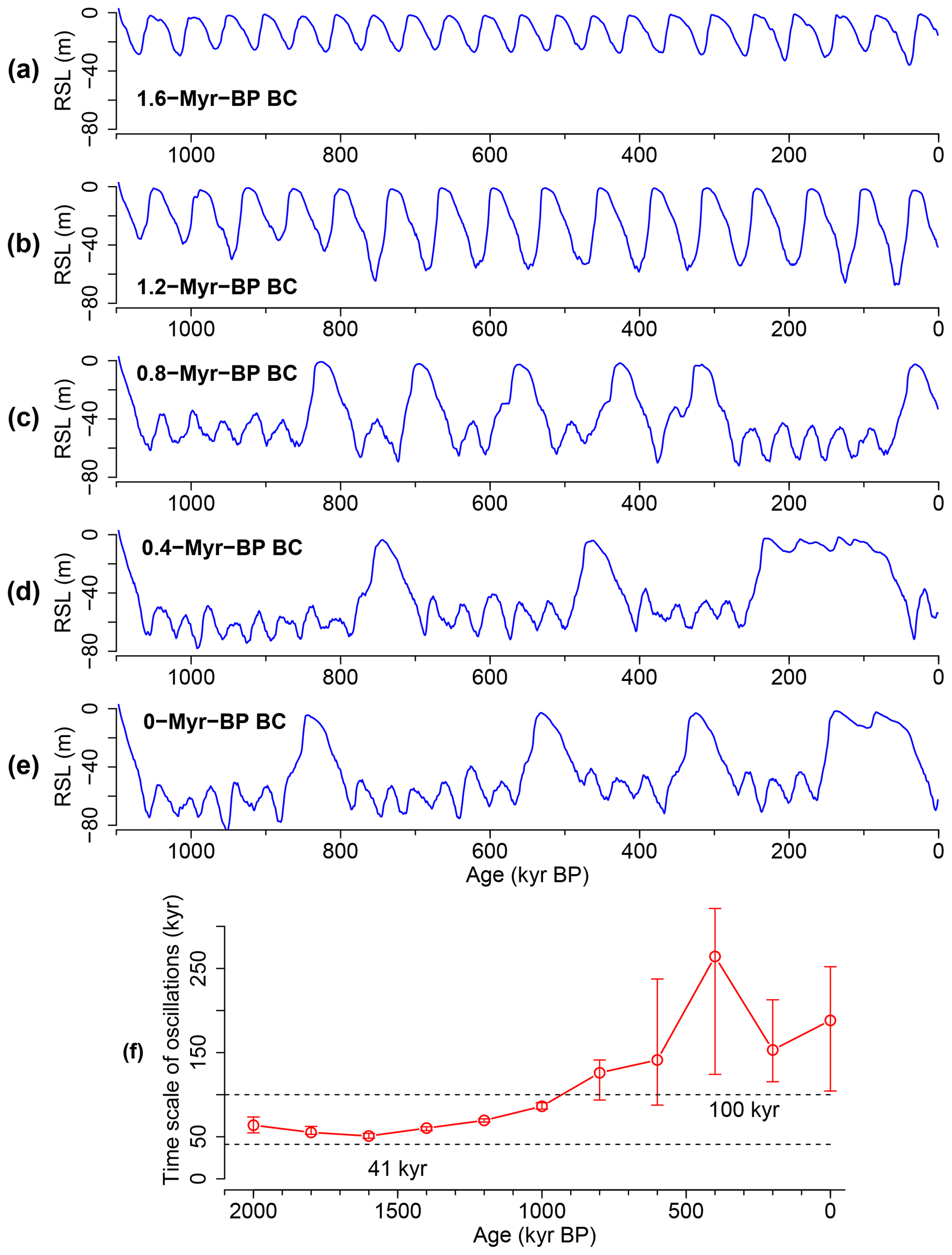
Figure 3 Gradual increase in the timescale of internal oscillations, inferred from simulations with fixed orbital configuration (zero eccentricity and mean obliquity). Simulated relative sea level (RSL) for different background conditions (BC) of volcanic-CO₂ outgassing rate and regolith cover corresponding to (a) 1.6, (b) 1.2, (c) 0.8, (d) 0.4 Myr and (e) 0 Myr BP. (f) The internal timescale as a function of age, from which the BC used for the simulation is taken. The timescale is derived from the PSD of the corresponding time series over 1000 kyr BP to present. The circles denote the medians, and the vertical bars show the interquartile range. The horizontal dashed lines indicate 41 and 100 kyr for reference.

The internal dynamics are investigated with unforced simulations for fixed orbital configurations. The configuration with zero eccentricity e=0 and mean obliquity $\mathit{\epsilon }=\mathrm{23.34}{}^{\circ }$ effectively gives an average seasonal insolation change (Fig. S5). This is reasonable since any insolation curve for a season and a latitude is well approximated by a linear combination of the obliquity ε, climatic precession esin ω and co-precession ecos ω (Imbrie and Imbrie, 1980). For this fixed orbital configuration, CLIMBER-2 exhibits self-sustained oscillations with timescales dependent on the BCs. Quasi-regular self-sustained oscillations with periodicity around 50 kyr arise for BC fixed at their values of 1.6 Myr BP (Fig. 2a). Less regular self-sustained oscillations with a timescale of a few hundred kiloyears arise for present-day BC (Fig. 2c). Overall, the timescale of self-sustained oscillations gradually increases when moving from ∼ 1.5 to ∼ 0.5 Myr BP BC (Fig. 3). This increase in the internal timescale is accompanied by an increase in the amplitude of the oscillations (i.e., intensification of glacials). However in these unforced simulations for e=0 and $\mathit{\epsilon }=\mathrm{23.34}{}^{\circ }$, the sea level variations are limited to ∼ 80 m (Fig. 3), which is smaller than that of the forced case (∼ 120 m). Similar lengthening of internal timescales also occurs for the present-day orbital configuration (Fig. S6) and for the orbital configuration at the Last Glacial Maximum (21 kyr BP) (Fig. S7). In those cases, much larger (∼ 250 m) and much longer (half-million-year scale) oscillations are observed for the post-MPT BCs, mainly due to the carbon cycle feedback (see below).

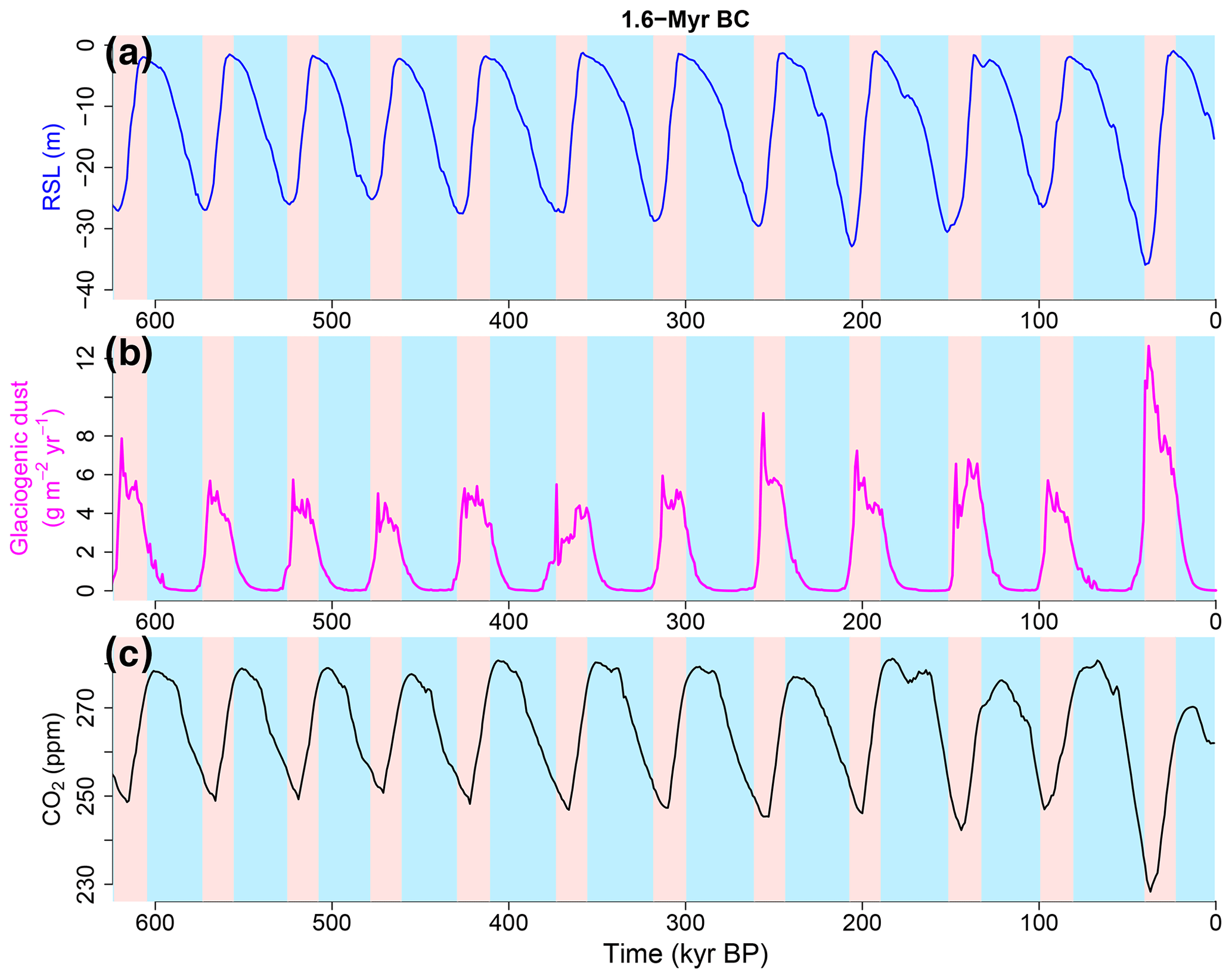
Figure 4 Self-sustained oscillations for the background condition (regolith cover and volcanic outgassing rate) at 1.6 Myr BP and a fixed orbital configuration (e=0 and $\mathit{\epsilon }=\mathrm{23.34}{}^{\circ }$). (a) Relative sea level (RSL). (b) Glaciogenic dust deposition rate. The mean value at (45^∘ N, 100^∘ E) and (55^∘ N, 100^∘ E). (c) Atmospheric CO₂ concentration. The oscillation period is about 50 kyr.

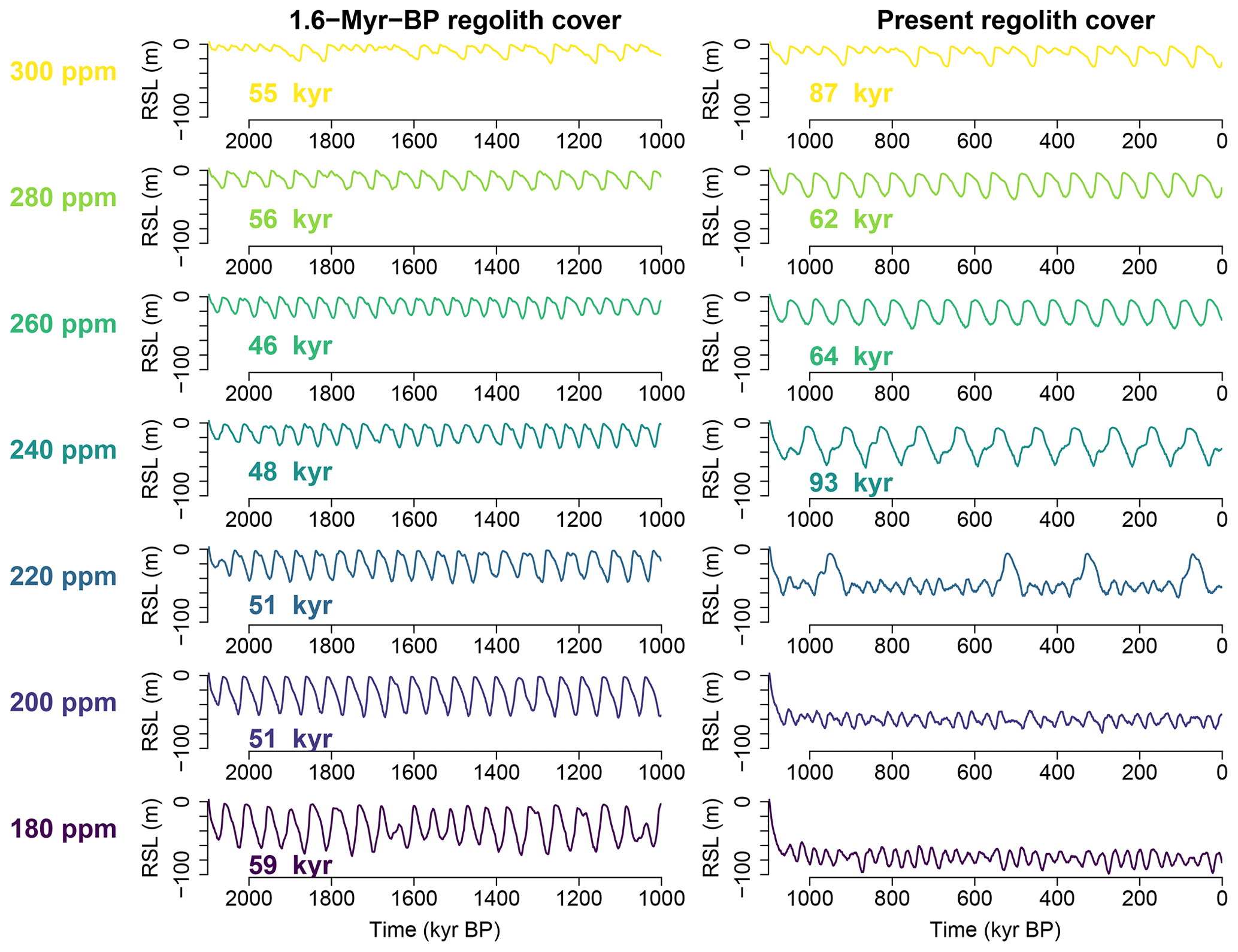
Figure 5 Relative sea level (RSL) simulated by CLIMBER-2 for fixed atmospheric CO₂ concentration and a fixed orbital configuration (e=0 and $\mathit{\epsilon }=\mathrm{23.34}{}^{\circ }$). Left column: simulations with 1.6 Myr BP regolith cover. Right column: those with the present regolith cover. All feedback processes except for the carbon cycle feedback are active. The number in each panel is the mean period of oscillations that reaches the sea level of 0 m.

The self-sustained oscillations of CLIMBER-2 found here are generated by various feedback processes described in previous studies (Ganopolski et al., 2010; Ganopolski and Calov, 2011; Brovkin et al., 2012; Ganopolski and Brovkin, 2017). The glaciogenic dust feedback and the carbon cycle feedback are especially crucial. Indeed, if the atmospheric CO₂ concentration is fixed to a constant value and if the glaciogenic dust feedback is switched off, the spontaneous oscillations cease, or, even if some fluctuations remain, their amplitudes are reduced (Fig. S8).

In the unforced simulation for the BC at their 1.6 Myr BP values, e=0 and $\mathit{\epsilon }=\mathrm{23.34}{}^{\circ }$ (Fig. 4), ice sheets nucleate and then grow facilitated by the ice albedo feedback. However, once the sea level reaches around −30 m, the ice sheets rapidly shrink due to an abrupt increase in glaciogenic dust deposition over the Northern Hemisphere ice sheets (Fig. 4b), which reduces the ice albedo and enhances ablation (Ganopolski et al., 2010). While the glaciogenic dust emissions are low during glaciation periods, high glaciogenic dust emissions continue throughout the deglaciation since the terrestrial sediments, which are eroded and transported to the margins of the ice sheets by basal ice sliding if the ice sheet base is at melting point, are exposed to the air when the ice sheets retreat. In the unforced simulation with 1.6 Myr BP BC, the period of self-sustained oscillations (∼ 50 kyr) is primarily set by ice sheet dynamics and the glaciogenic dust feedback. The carbon cycle feedback slightly modifies the oscillation amplitude but does not affect the oscillation period significantly. Indeed in the unforced simulations with fixed atmospheric CO₂ concentrations over 180–300 ppm and the 1.6 Myr BP BC (Fig. 5, left), the period of self-sustained oscillations stably remains in a narrow range between 45 and 60 kyr.

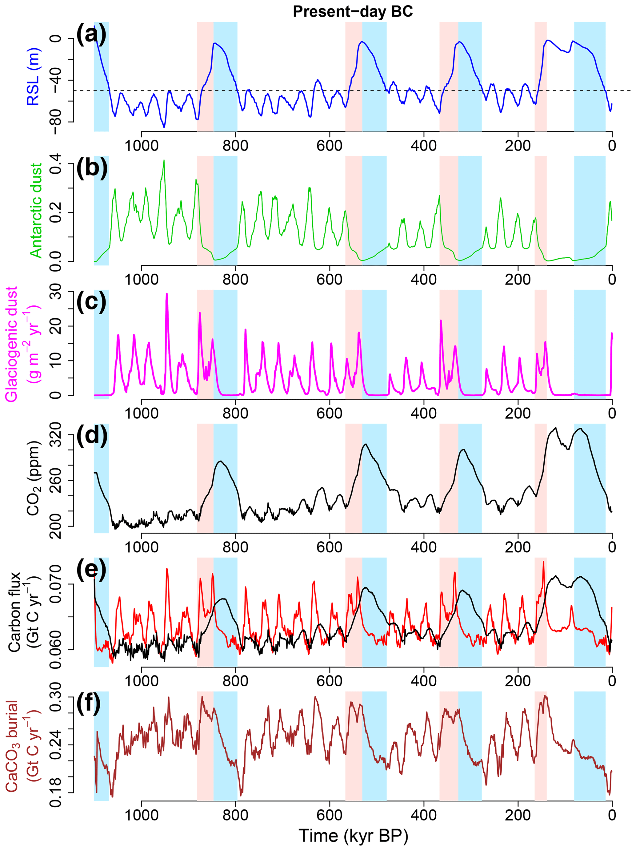
Figure 6 Self-sustained oscillations for the present background condition (regolith cover and volcanic outgassing rate) and fixed orbital configuration (e=0 and $\mathit{\epsilon }=\mathrm{23.34}{}^{\circ }$). (a) Relative sea level (RSL). The horizontal dashed line indicates the RSL of −50 m, below which the dust-borne iron fertilization of the Southern Ocean is enhanced in the model. The mean periodicity is about 250 kyr. (b) Antarctic dust deposition in relative units as a proxy for the iron flux over the Southern Ocean. (c) Glaciogenic dust deposition rate. The mean value at (45^∘ N, 100^∘ E) and (55^∘ N, 100^∘ E). (d) Atmospheric CO₂ concentration. (e) Carbon fluxes: the variable volcanic outgassing rate (red) and the consumption of atmospheric CO₂ due to terrestrial weathering of silicate (black). (g) CaCO₃ burial in the deep ocean and on the ocean shelf. It shows that the carbonate (alkalinity) pump is strengthened in the direction releasing CO₂ during glacials on average, as well as during terminations.

In the unforced simulation with the present-day BC, e=0 and $\mathit{\epsilon }=\mathrm{23.34}{}^{\circ }$ (Fig. 6), the carbon cycle feedbacks play a crucial role in setting the timescale and the amplitude of spontaneous oscillations. Starting from the sea level of zero, the ice sheets nucleate and grow in conjunction with a decrease in the atmospheric CO₂ (Fig. 6a and d). As the sea level decreases below −50 m, enhanced dust deposition in the Southern Ocean induces a further rapid reduction in CO₂ via the iron fertilization effect, which causes a further ice volume increase (Fig. 6a and b). However, then a sudden increase in glaciogenic dust deposition over the Northern Hemisphere ice sheets interrupts their growths by reducing albedo and enhancing ablation (Fig. 6a and c). These counteracting effects keep the sea level around −80 to −50 m for 100–200 kyr. During the glacial state, the atmospheric CO₂ increases on average, very gradually with a rate on the order of ∼ 0.1 ppm kyr⁻¹ (Fig. 6d), due to the following feedbacks: the volcanic outgassing rate slightly increases on average, responding to sea level rise (Fig. 6e, red) (cf. Huybers and Langmuir, 2009), while on the other hand, the terrestrial silicate weathering consuming atmospheric CO₂ weakens during glacials (Fig. 6e, black). Also the carbonate (alkalinity) pump is strengthened in the direction of releasing CO₂ during glacials on average as well as during terminations, as shown by the increase in CaCO₃ burial (Fig. 6f). Finally the ice sheets retreat with the help of the glaciogenic dust deposition and the rapid atmospheric CO₂ rise, which is sustained during the deglaciation. In sum, the few-hundred-kiloyear self-sustained oscillations for the present-day BC emerge from the interaction of ice sheet dynamics, glaciogenic dust and carbon cycle feedbacks. Note that self-sustained oscillations arise even without the glaciogenic feedback if the carbon cycle feedback is active, but the maximum ice volume becomes much larger and the periodicity much longer (Fig. S9).

There is a weak warming trend superimposed on the self-sustained oscillations (Fig. 6) due to a long-term CO₂ increase. This reflects long transient dynamics, where the carbon fluxes are still slightly imbalanced. We suppose that the system will eventually achieve a more regular limit cycle behavior without a drift. However, it takes at least more than 1 million years. Therefore, we consider that the oscillatory behavior with the subtle drift is an essential character underlying the modeled ice age cycles.

The period of self-sustained oscillations for the present-day BC (∼ 250 kyr on average) is decomposed into two parts: the periods for the buildup and collapse of ice sheets and those for glacials and interglacials. The joint period for the buildup and collapse of ice sheets is 80–90 kyr and relatively stable (Fig. 6), which is roughly estimated as the maximum size of ice volume divided by the difference between accumulation and ablation rate. On the other hand, the duration of glacials ranges between 100 and 250 kyr depending on the glacial atmospheric CO₂ concentration (compare the first two glacial periods with the last two in Fig. 6). A similar effect of CO₂ is also confirmed in the simulations with fixed atmospheric CO₂ concentration, where the glacial ice sheets are more stable (that is, the glacial duration becomes longer) if the prescribed CO₂ concentration is lower than a critical level of ∼ 220 ppm (Fig. 5, right). In sum, the few-hundred-kiloyear periodicity for the present-day BC is determined jointly by the timescale of ice sheet evolution and the length of glacials and interglacials, which is sensitive to the atmospheric CO₂ concentration.

3.3 Frequency entrainment

It remains to be explained how the change in the internal timescale leads to the observed frequency change across the MPT. If we compare the spectra of forced simulations with those of corresponding unforced ones (Fig. 2), we find that the spectral powers of forced simulations are entrained at one or few astronomical frequencies near the frequency of internal self-sustained oscillations. The theory of synchronization (Pikovsky et al., 2003) may provide a general explanation for these observations. In essence, frequency entrainment (i.e., synchronization) tends to occur near the internal frequency as long as the external forcing is moderate (Fig. S1 and Appendix A).

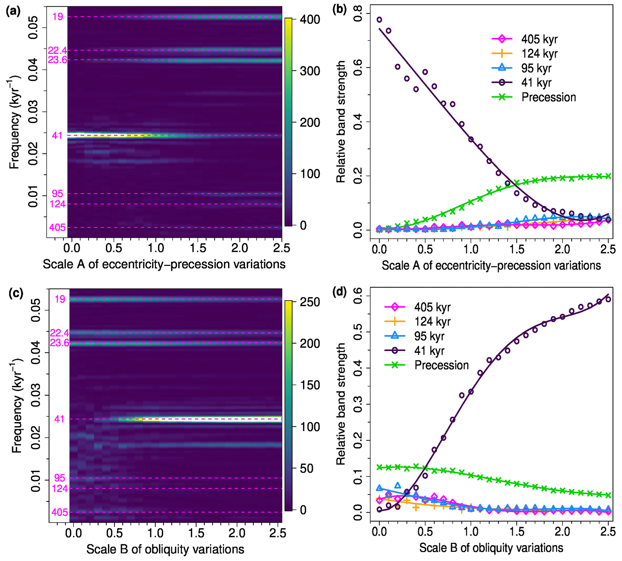
Figure 7 Sensitivity experiments with respect to the astronomical forcing under pre-MPT (1.6 Myr BP) background condition. (a) Averaged normalized power spectral density (PSD) of three CLIMBER-2 simulations as a function of the scale A of the eccentricity and climatic precession. The horizontal dashed lines (magenta) and associated numbers indicate the major astronomical frequencies (corresponding to periodicities at 405, 124, 95 and 41 kyr). (b) Relative band strengths P₄₀₅, P₁₂₄, P₉₅, P₄₁ and P_precession as functions of A, obtained from the PSD in (a) (cf. Appendix C). The lines are fourth-order polynomial fits to the data points. (c) Averaged normalized PSD of the CLIMBER-2 simulations as a function of the scale B of the obliquity. (d) Relative band strengths as functions of B, obtained from the PSD in (c).

Consistent with synchronization theory, the oscillations before the MPT are entrained by the 41 kyr obliquity cycles, due to the proximity of the internal periodicity (around 50 kyr) to the 41 kyr obliquity periodicity (Fig. 2a and b). The oscillations after the MPT are entrained by the eccentricity periodicities at 95, 124 and 405 kyr because the several-hundred-kiloyear timescales of internal oscillations for post-MPT BCs are closer to those eccentricity periodicities than to the much smaller obliquity periodicity (Fig. 2c and d). Reflecting temporarily desynchronized epochs in the simulated glacial cycles after the MPT, the magnitudes of the 95, 124 and 405 kyr band powers depend on the realizations of simulated sequences. If the ensemble average is taken for the spectra (from 27 simulations), the 95 kyr band power is the strongest (Fig. S2b). For some realizations, a noticeable peak appears between 124 and 95 kyr (Fig. S2). It might be linked with the 107 kyr peak that arises as a higher-order combination tone of 95 and 405 kyr eccentricity periodicities ($\mathrm{1}/\mathrm{107}\simeq \mathrm{1}/\mathrm{95}-\mathrm{1}/(\mathrm{2}\times \mathrm{405})$) (Rial, 1999, and Appendix A), but note that the 107 kyr peak is still not well established since it is so close to 95 and 124 kyr peaks.

The frequency entrainment at the eccentricity frequencies does not result from the eccentricity forcing itself but results from the climatic precession forcing esin ω (ecos ω), whose amplitude is modulated by the eccentricity cycles. As shown in Fig. B1 in Appendix B, the deglaciations occur near peaks of climatic precession (i.e., boreal summer insolation peaks) in rising or high phases of eccentricity (Raymo, 1997; Ridgwell et al., 1999; Ganopolski and Calov, 2011; Abe-Ouchi et al., 2013).

Given that the eccentricity has the strongest power at 405 kyr over the last 1 Myr, it is unclear why – and actually rather surprising that – the internal oscillations with a timescale of a few hundred kiloyears are entrained most strongly by the 95 kyr periodicity and not by 405 kyr. In what follows we show that the 41 kyr obliquity variations play a crucial role in synchronizing the climate system to the 95 kyr rather than the 405 kyr periodicity, via a new nonlinear phenomenon that we term vibration-enhanced synchronization.

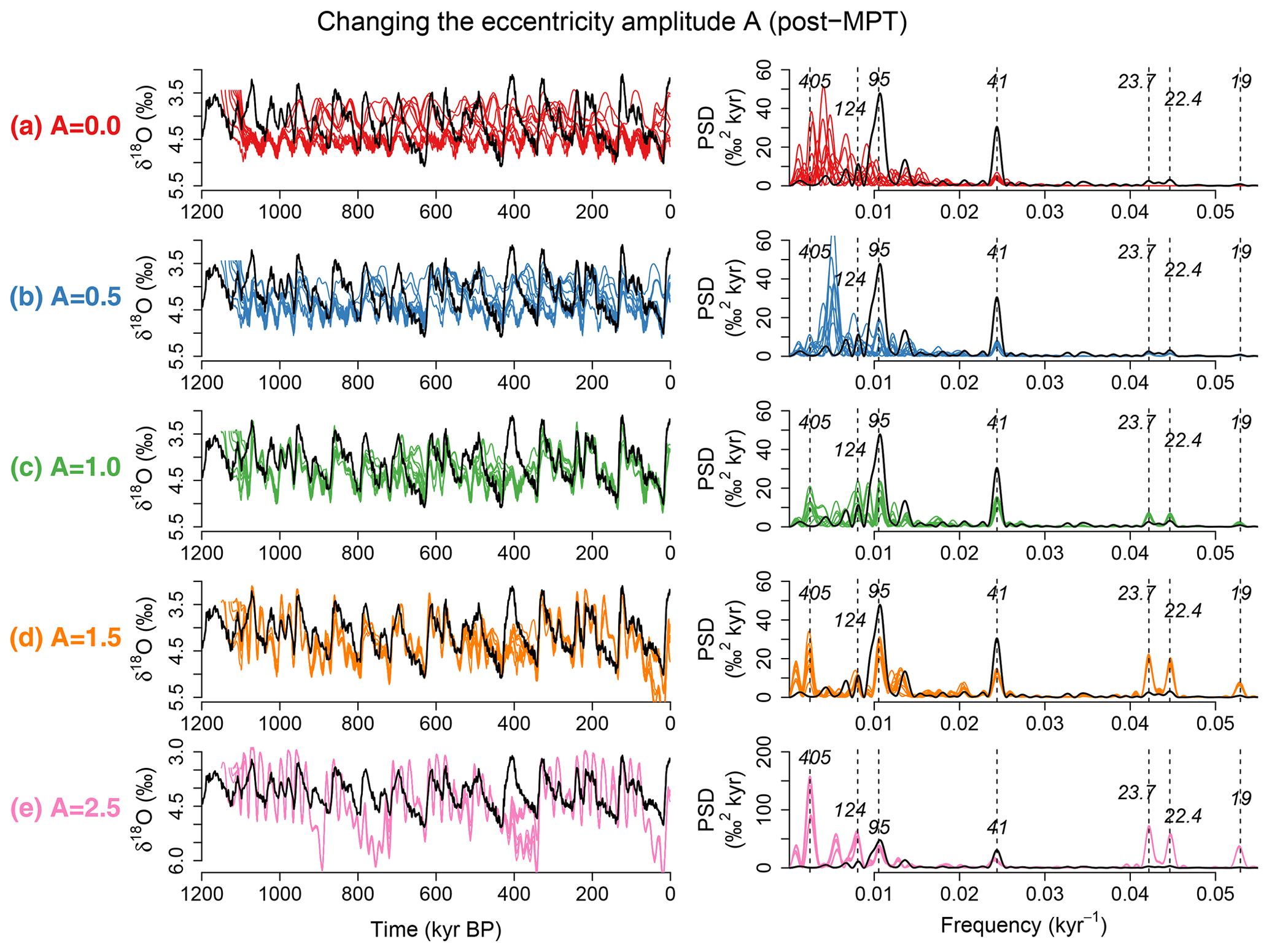
Figure 8 Sensitivity experiments changing the scale A of the eccentricity (Laskar et al., 2004) (and hence of climatic precession) under post-MPT background conditions (see text). Ten simulated δ¹⁸O time series starting from different initial times (i.e., different orbital configurations) are shown for different values of A on the left of (a) to (e). The black line is the LR04 δ¹⁸O record (Lisiecki and Raymo, 2005). The corresponding power spectral densities (PSD) are shown on the right. The dashed vertical lines and italic numbers indicate the positions of major astronomical frequencies and their periods (Laskar et al., 2004). For A smaller than the realistic values A=1, variability at timescales of several hundred kiloyears dominates. Near the realistic value A=1, the glacial cycles synchronize to the 95 kyr eccentricity cycle. For A much larger than 1, the system resonates with the 405 kyr eccentricity cycles.

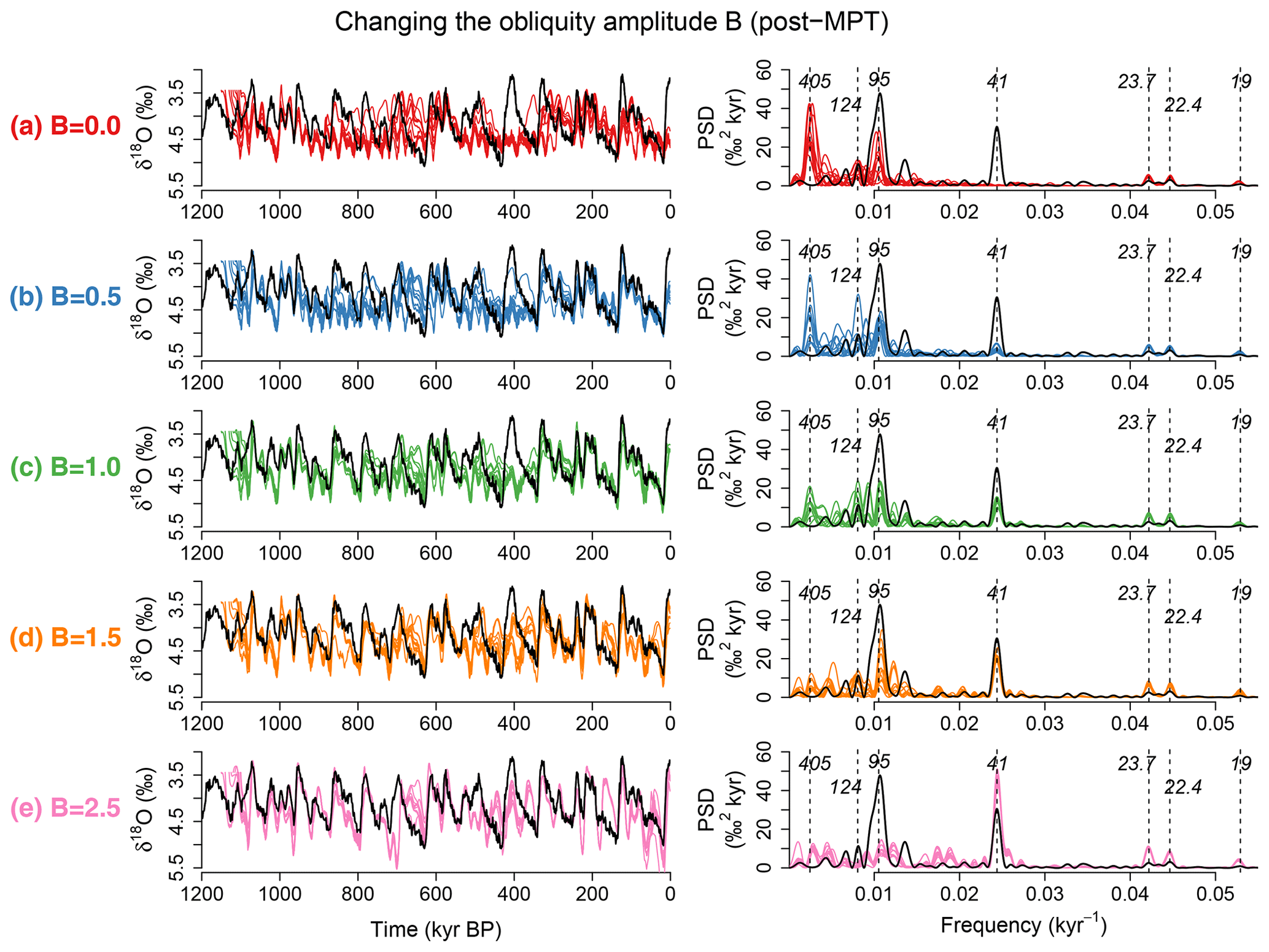
Figure 9 Sensitivity experiments changing the scale B of the obliquity (Laskar et al., 2004) under the post-MPT background condition (see text). Ten simulated δ¹⁸O series starting from different initial times (i.e., different orbital configurations) are shown for different values of A on the left of (a) to (e). The black line is the LR04 δ¹⁸O record (Lisiecki and Raymo, 2005). The corresponding power spectral densities (PSDs) are shown on the right. The dashed vertical lines and italic numbers indicate the positions of major astronomical frequencies and their periods (Laskar et al., 2004). The increase in the scale B of the obliquity variations reduces the 405 kyr power and makes the 95 kyr power dominate – the phenomenon of vibration-enhanced synchronization.

4 Cooperative effect of the changes in astronomical elements

In order to investigate the respective roles of climatic precession and obliquity forcing in producing the dominant 41 and ∼ 100 kyr periodicities before and after the MPT, we conduct two sets of additional sensitivity experiments with BC fixed at pre-MPT (i.e., 1.6 Myr BP) and at post-MPT (i.e., present-day) values, respectively. First, we run CLIMBER-2 simulations with the actual obliquity ε(t) and a scaled eccentricity Ae(t), with $\mathrm{0}\le A\le \mathrm{2.5}$. The climatic precession is accordingly scaled (i.e., Aesin ω), but its phase is the same as the real variation. Second, we run the model with the true eccentricity and climatic precession, but with scaled obliquity ${\mathit{\epsilon }}^{\prime }\left(t\right)=\mathrm{23.34}{}^{\circ }+B\left(\mathit{\epsilon }\right(t)-\mathrm{23.34}{}^{\circ })$, with $\mathrm{0}\le B\le \mathrm{2.5}$. The real-world forcing corresponds to A=1 and B=1. The PSDs are calculated for the simulated δ¹⁸O time series for varying A and B. To get clearer insights about the changes in PSDs, we investigate the ensemble-averaged normalized PSD and the ensemble-averaged relative band strength for changing combinations of A and B (see Appendix C).

Figure 10 Sensitivity experiments with respect to the astronomical forcing under post-MPT background conditions. (a) Averaged normalized power spectral density (PSD) of 10 CLIMBER-2 simulations as a function of the scale A of eccentricity and climatic precession. The horizontal dashed lines (magenta) and associated numbers indicate the major astronomical frequencies (corresponding to periodicities at 405, 124, 95 and 41 kyr). (b) Relative band strengths P₄₀₅, P₁₂₄, P₉₅, P₄₁ and P_precession as functions of A, obtained from the PSD in (a) (cf. Appendix C). The lines are third-order polynomial fits to the data points. (c) Average PSD of the CLIMBER-2 simulations as a function of the scale B of the obliquity. (d) Relative band strengths as functions of B, obtained from the PSD in (c).

4.1 Pre-MPT background conditions

First, the scale A of eccentricity–climatic precession forcing is changed while keeping the real obliquity forcing. The time series and spectra for several values of A are shown in Fig. S10; the summary plots are in Fig. 7a and b. As long as the scale A of eccentricity–climatic precession forcing is moderate (A≲1.5), the 41 kyr power simply dominates; for A≳1.5 the mean precession-band power surpasses the 41 kyr band power (Fig. 7a and b).

Second, we change the scale B of obliquity variations while keeping the actual eccentricity-precession forcing (see Fig. S11 for the time series and spectra for several values of B). If the obliquity forcing is absent or very weak (B≲0.3), the sequences of simulated glacial cycles starting from different initial conditions are not fully synchronized to each other and have dominant powers at the precession bands (Fig. S11a). However, if the obliquity forcing is strong enough (B≳0.5), the sequences of simulated glacial cycles starting from different initial conditions are synchronized well to each other and to the 41 kyr obliquity cycles (Fig. S11). The 41 kyr band power increases rather rapidly over $\mathrm{0.5}\lesssim B\lesssim \mathrm{1.2}$, exceeding the average precession-band power (Fig. 7d). This nonlinear increase in the 41 kyr power with B can be partly explained as a synchronization. However, the amplitude of simulated glacial-cycle oscillations moderately increases as the forcing amplitudes A and B increase (Figs. S10 and S11). This is the aspect of linear response.

4.2 Post-MPT background conditions

First, the eccentricity–climatic precession is scaled while keeping the actual obliquity forcing. The δ¹⁸O series and spectra for several values of A are plotted in Fig. 8, and the summary plots are given in Fig. 10a and b. In the absence of eccentricity–climatic precession change (A=0), the obliquity forcing alone cannot constrain the sequence of glacial cycles, and the PSDs are not substantially different from those of internal oscillations, having the largest powers in between the 400 and 100 kyr bands (Fig. 8a). If the scale A of eccentricity is increased up to around A=1, the oscillations are roughly synchronized to the 95 kyr periodicity, which is strongest statistically, although also the 124 and 405 kyr bands may receive a noticeable fraction of the spectral power, depending on initial conditions (Figs. 8c and S2 for an enlarged version). For A>1.8, the 405 kyr band receives the maximum strength (Fig. 10a and b). For the extreme case A=2.5, huge ice sheets appear near every 400 kyr eccentricity minimum (Fig. 8e). The system achieves a synchronized state with prominent ∼ 100 kyr periodicity for a realistic scale of the eccentricity–climatic precession forcing (A≈1), and the dynamics shift toward a nonlinear resonance mode with the 405 kyr eccentricity cycles for much larger A. It is worth mentioning that the relative strength of the 41 kyr power is largest near A=1 (Fig. 10b).

Second, the scale B of obliquity variations is varied while we keep the actual eccentricity–climatic precession forcing (Figs. 9, 10c and d). In the absence of obliquity forcing (B=0), glacial–interglacial cycles are likely to occur when the eccentricity is large, giving rise to a roughly 400 kyr periodicity (Fig. 9a); the 95 kyr mode still exists, while it is weaker than the 405 kyr mode. As B increases, the 405 kyr band power is suppressed, and the 41 kyr band power increases. Statistically, the 95 kyr power becomes strongest in the range of $\mathrm{0.7}\lesssim B\lesssim \mathrm{1.2}$ (Fig. 10c and d). This is nontrivial because the dominance of 95 kyr periodicity is enabled by the 41 kyr obliquity forcing, which is directly related to neither 95 kyr nor 405 kyr periodicity. We call this novel nonlinear mechanism vibration-enhanced synchronization (see discussion below). While the enhancement of the ∼ 100 kyr power by the 41 kyr obliquity forcing is consistent with previous modelling studies (Ganopolski and Calov, 2011; Abe-Ouchi et al., 2013), we have further shown that ∼ 100 kyr cycles become dominant only for a limited amplitude range of obliquity variations (Fig. 11b).

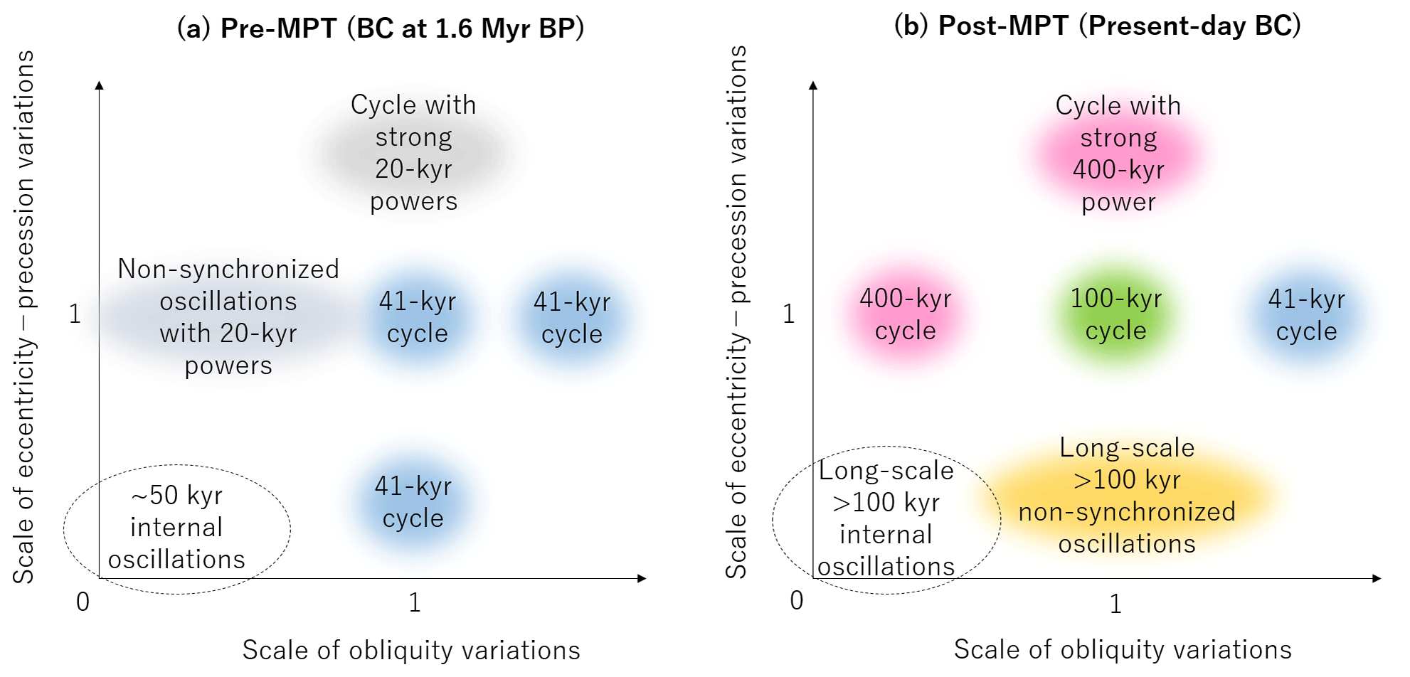
Figure 11 Summary diagrams illustrating various dynamical regimes realized by CLIMBER-2 for different scales of obliquity and eccentricity–climatic precession variations. (a) Pre-MPT background conditions (BCs), specifically 1.6 Myr BP BC. The system exhibits internal oscillations of ∼ 50 kyr periodicity in the absence of forcings. For a realistic or smaller scale of eccentricity–precession forcing, the simulated glacial cycles synchronize to the 41 kyr obliquity forcing if the scale of obliquity variations is realistic or larger. (b) Post-MPT BC, i.e., for the present day. The unforced system exhibits spontaneous oscillations of several hundred kiloyears in scale. The ∼ 100 kyr cycles occur only for realistic scales of obliquity and eccentricity–precession variations.

5 Summary and discussion

We have reported self-sustained oscillations and their synchronization to the astronomical forcing in glacial cycles simulated by the Earth system model of intermediate complexity CLIMBER-2, specifically the model version also used in Willeit et al. (2019a). Based on the results of forced and unforced experiments, we have explained the rhythms of simulated glacial cycles from the perspective of the synchronization principle. We have found that when fixing astronomical parameters at their reasonable averages, the model exhibits self-sustained oscillations of periodicities around 50 kyr under pre-MPT background conditions regarding volcanic-CO₂ outgassing rate and the regolith cover. Under post-MPT background conditions, the unforced model exhibits spontaneous oscillations at timescales of a few hundred kiloyears. The glaciogenic dust feedback and the carbon cycle feedback play key roles in the self-sustained oscillations. Before the MPT, the glacial cycles synchronize to the 41 kyr obliquity cycles since the internal oscillations have periodicity (∼ 50 kyr) relatively close to 41 kyr. This follows the universal principle of synchronization: frequency entrainment occurs if the frequency of internal self-sustained oscillations is in the neighborhood of the frequency of external forcing (Pikovsky et al., 2003). After the MPT the timescale of internal oscillations becomes too long to follow the 41 kyr obliquity cycle, and the glacial cycles synchronize to the ∼ 100 kyr eccentricity cycles (statistically most likely at the 95 kyr band). In this case, via vibration-enhanced synchronization, the 41 kyr obliquity variations enable synchronization of oscillations at the ∼ 100 kyr eccentricity band (Figs. 9 and 10d).

We termed the synchronization to the ∼ 100 kyr eccentricity cycles, enhanced by 41 kyr obliquity forcing, as vibration-enhanced synchronization since it can be seen as a deterministic analogue of noise-enhanced synchronization of chaotic oscillations to a weak periodic signal (Zhou et al., 2003). In the latter study, the authors numerically and experimentally found that chaotic oscillations in a CO₂ laser synchronize to a weak periodic forcing if a certain magnitude of dynamical noise is added to the system. A similar enhancement of synchronization is also found in human brain waves, which is called noise-induced entrainment (Mori and Kai, 2002). In the early 1980s, Benzi et al. (1982) and Nicolis (1981) independently proposed the idea of stochastic resonance, suggesting that glacial–interglacial transitions can resonate with the weak ∼ 100 kyr eccentricity forcing if the ambient noise has a certain amplitude (for several extensions of the stochastic resonance idea, see Matteucci, 1989; Ditlevsen, 2010; Pelletier, 2003; and Bosio et al., 2022). The vibration-enhanced synchronization found here is similar to the stochastic resonance, but deterministic.

Our results suggest that the MPT is due to the gradual increase in the period of the climate system's internal oscillations, leading to a transition from synchronizing to the 41 kyr obliquity to synchronizing to the ∼ 100 kyr eccentricity cycles. This is consistent with some previous studies (Nyman and Ditlevsen, 2019; Ashkenazy and Tziperman, 2004; Mitsui et al., 2015) and also coherent with the gradual increase in the deglaciation threshold (Paillard, 1998; Tzedakis et al., 2017; Berends et al., 2021; Legrain et al., 2023). Our theory is, however, different from the Hopf bifurcation scenario, which assumes the onset of self-sustained (limit cycle) oscillations around the timing of the MPT (Ghil and Childress, 1987; Maasch and Saltzman, 1990; Crucifix, 2012), since the CLIMBER-2 simulations exhibit internal self-sustained oscillations before the MPT. Note that there are many explanations of the MPT not invoking self-sustained oscillations, e.g., Huybers and Tziperman (2008), Daruka and Ditlevsen (2016), and Verbitsky et al. (2018) as well as those mentioned in the introduction section above. Further studies assessing the dynamical mechanisms of the MPT are necessary.

There are some caveats to our work. The CLIMBER-2 model in its present setting has some problems in simulating the deglaciation around 430 kyr BP at Termination V. The last deglaciation is incomplete, leaving the present interglacial colder than observed. The North American ice sheet nucleates at the preindustrial CO₂ level (Figs. 5 and S8). Thus the present model setting, calibrated on several-hundred-kiloyear glacial cycles, could be biased toward glacial states. Some parameters and parameterizations including the glaciogenic dust deposition process are only weakly constrained by empirical data, as mentioned in Ganopolski et al. (2010). Therefore, it is important to examine in future work if similar self-sustained oscillations and synchronization phenomena could be observed in a more recent version of CLIMBER-X (Willeit et al., 2022, 2023) as well as in other comprehensive models.

The CLIMBER-2 version (Willeit et al., 2019a; W19) used in this study is slightly different from the earlier version by Ganopolski and Brovkin (2017) (GB17). Specifically, W19 includes an interactive dust cycle, a deep permafrost model and a slightly different present-day regolith mask (see Supplement). In contrast to W19, the GB17 version is not self-oscillatory for a wide range of parameters. Nevertheless, the GB17 version exhibits self-sustained oscillations with the constant orbital forcing and CO₂ for the regolith covering all the continents in a rather narrow range of CO₂ concentrations (220–240 ppm) (see the comment by Andrey Ganopolski: https://doi.org/10.5194/esd-2023-16-CC1). That is, CLIMBER-2 has the capacity to exhibit self-sustained oscillations by subtle changes in model components or parameters. Given that GB17 or other models which are not self-oscillatory exhibit clear ∼ 100 kyr cycles, we do not claim that the self-sustained oscillations are mandatory for the ∼ 100 kyr cycles. Instead we have proposed that if self-sustained oscillations exist, the dominant frequency of glacial cycles under the forcing is determined in relation to the period of the self-sustained oscillations.

Recently, Watanabe et al. (2023) have conducted similar sensitivity experiments changing the amplitudes of orbital variations in the IcIES-MIROC model (Abe-Ouchi et al., 2013), which is a three-dimensional thermomechanical ice sheet model with parameterized climate feedback obtained from pre-run snapshot by a coupled general circulation model (MIROC). In their simulations, if the amplitude of the climatic precession is reduced to 20 % (while the true obliquity is used), the dominance of the 41 kyr cycles is lost in the Early Pleistocene, and glacial cycles having a strong ∼ 100 kyr power arise. This strong sensitivity to the precession forcing in the 41 kyr cycles simulated by the IcIES-MIROC is contrasted with the weak sensitivity to the precession forcing in the 41 kyr cycles simulated by CLIMBER-2 (Figs. 7b and S10). This difference may be related to the presence of internal self-sustained oscillations with periodicity close to 41 kyr in CLIMBER-2 (Fig. 2a) and the absence of the internal oscillations in IcIES-MIROC (Watanabe et al., 2023). Nevertheless, our results with CLIMBER-2 do not contradict the observed influences of both climatic precession and obliquity forcing on the Early Pleistocene 41 kyr glacial cycles (Liautaud et al., 2020; Barker et al., 2022; Watanabe et al., 2023). Indeed, the simulated sequence of pre-MPT glacial cycles and its spectra are close to those of the δ¹⁸O record if the amplitude of the climatic precession is realistic (Figs. S12 and S13).

We have described the dominant rhythms of glacial cycles as the result of synchronization of internal oscillations to the astronomical forcing. It should however be mentioned that, in the CLIMBER-2 simulations, the astronomical forcing not only adjusts the frequency of glacial cycles but also increases the amplitude of oscillations and makes the shape of the cycles more asymmetric. In this sense the form of synchronization of glacial cycles slightly deviates from the prototypical notion of synchronization, i.e., the frequency and phase adjustment of oscillators by weak forcing (Pikovsky et al., 2003). As stated in the introduction, the distinction between synchronization and nonlinear response can be subtle when the external forcing is strong in comparison to the internal dynamics. After the MPT, in agreement with the proxy records, CLIMBER-2 simulations show dominant ∼ 100 kyr cycles, but they also exhibit more rapid oscillations, for example, over one precession cycle around 230 kyr BP and over two precession cycles or one obliquity cycle around 600 kyr (Fig. B1). These rapid cycles may be seen as more direct responses to the strong precession forcing associated with strong eccentricity at those time epochs, rather than as the result of synchronization of 100 kyr scale spontaneous oscillations. Therefore, the glacial–interglacial cycles over the last 1 Myr show different facets over time: the synchronization of internal self-sustained oscillations to the ∼ 100 kyr eccentricity cycles and the forced responses to the strong precession forcing associated with strong eccentricity (Imbrie et al., 1992, 1993; Gildor and Tziperman, 2000; Lisiecki, 2010).

Based on the CLIMBER-2 simulations, we have suggested that the ∼ 100 kyr glacial cycles over the last 1 Myr are realized by cooperative action of eccentricity–climatic precession forcing and obliquity forcing; this is only possible in a specific range of the scales of orbital variations (Fig. 11). In the absence of the eccentricity–climatic precession forcing, the obliquity forcing alone cannot synchronize the glacial cycles, and the timescales of oscillations are much larger than ∼ 100 kyr. The 95 kyr power dominates if the amplitude of climatic precession is realistic. However, the 405 kyr band becomes strongest for larger amplitudes of eccentricity–climatic precession forcing and dominates in the absence of obliquity cycles. The increase in the obliquity amplitude weakens the 405 kyr power and makes the 95 kyr power dominant as long as the obliquity amplitude is realistic. If the obliquity amplitude is substantially larger than realistic values, the 41 kyr power simply dominates. Via the phenomenon of vibration-enhanced synchronization the 41 kyr obliquity forcing thus helps the synchronization of the Earth's climate system to the ∼ 100 kyr eccentricity cycles.

Appendix A: Frequency entrainment (synchronization)

When a self-sustained oscillator with frequency f₀ is subject to an external forcing with frequency f_e, the frequency of oscillations under the forcing, f_r, can be entrained to f_e (i.e., f_r=f_e). This phenomenon is called frequency entrainment (or frequency locking) and is ubiquitously observed in natural or human-made oscillating systems (Pikovsky et al., 2003). This frequency entrainment occurs within a finite range of frequency detuning f_e−f₀, which is typically wider if the forcing is stronger (Fig. S1). If the internal frequency f₀ is far away from the external frequency f_e but close to a simple harmonic $(m/n)f_{\mathrm{e}}$ ($m,n\in \mathbb{N}$), the higher-order m:n synchronization can occur at $(m/n)f_{\mathrm{e}}$ (i.e., $f_{\mathrm{r}}=(m/n)f_{\mathrm{e}}$). On the other hand the higher-order synchronization has a narrower entrainment region and is less likely than a lower-order one (Fig. S1). If the external forcing has multiple frequencies (f_j, f_k and so on), the entrainment can occur at one of those frequencies, their harmonics $(m/n)f_j$ or a combination tone (e.g., $(m/n)f_j\pm (l/n)f_k$) close to the internal frequency f₀.

Appendix B: Simulated deglaciations at climatic precession peaks

In CLIMBER-2 simulations over the last 1 Myr, the major deglaciations appear to be triggered by climatic precession peaks corresponding to marked boreal summer insolation peaks in rising or high phases of eccentricity (Fig. B1), consistent with some previous proposals (Raymo, 1997; Ridgwell et al., 1999; Ganopolski and Calov, 2011; Abe-Ouchi et al., 2013). In many cases, a high or above-average obliquity assists the deglaciation (cf. Tzedakis et al., 2017, and vibration-enhanced synchronization proposed here). The frequency entrainment at eccentricity frequencies occurs via the synchronization of the few-hundred-kiloyear self-sustained oscillations with the ∼ 100 kyr scale amplitude modulation of climatic precession by the eccentricity change.

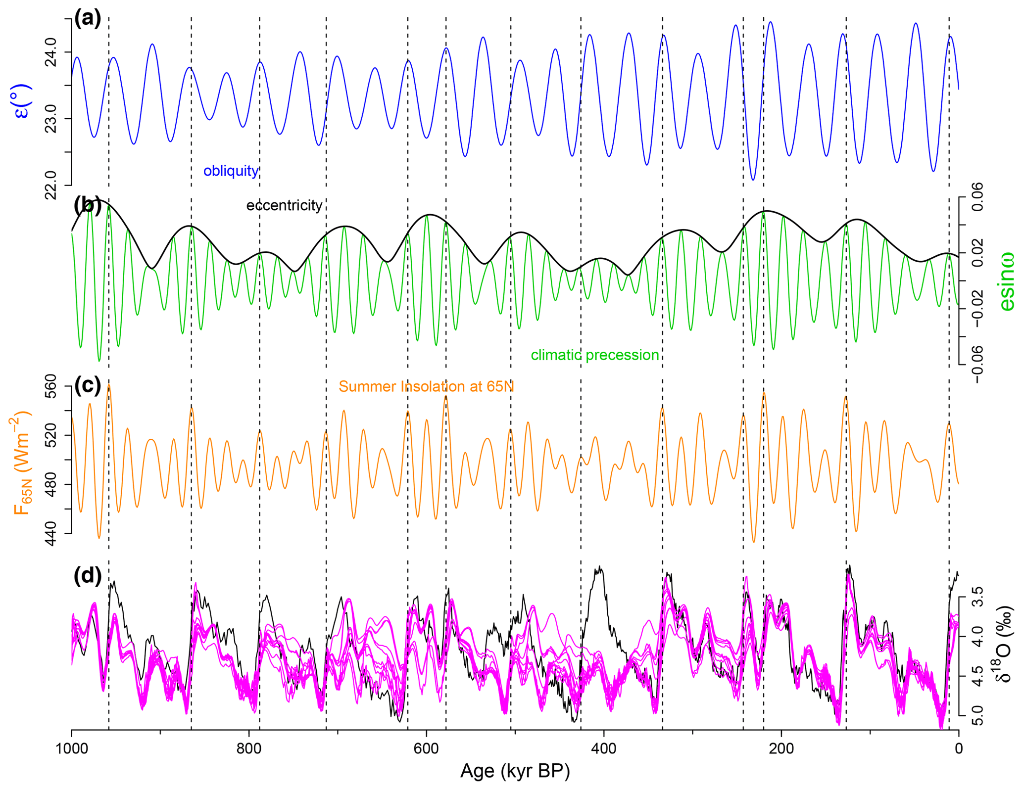
Figure B1 Simulated deglaciations at climatic precession peaks. (a) Obliquity (blue). (b) Climatic precession (green) and eccentricity (black). (c) Boreal summer solstice insolation at 65^∘N. (d) LR04 δ¹⁸O stack (Lisiecki and Raymo, 2005) (black) representing glacial–interglacial cycles during the last 1 Myr and corresponding CLIMBER-2 δ¹⁸O simulations (magenta) under the present background condition regarding the volcanic outgassing rate and the regolith cover. Ten simulations starting from slightly different initial conditions are shown. Note that the vertical axis is reversed so that larger δ¹⁸O values, corresponding to colder conditions, are displayed on the lower side. The major deglaciations occur near peaks of climatic precession (i.e., boreal summer insolation peaks), indicated by dashed lines, in rising or high phases of eccentricity. The astronomical parameters are from Laskar et al. (2004).

Appendix C: Power spectral density

The power spectral densities (PSDs) S(f) of different time series are estimated via periodograms (Bloomfield, 2004), which are computed with the R function spec.pgram (R Core Team, 2020). In particular when we focus on the relative strength of spectral peaks, we use the normalized PSD, defined as $S^N\left(f\right)=S\left(f\right)/{\int }_{\mathrm{0}}^{\mathrm{\infty }}S\left(f\right)\mathrm{d}f$. A split cosine bell taper is applied to 10% of the data at the beginning and end of the time series in order to minimize the effect of the discontinuity between the beginning and end of the time series (Bloomfield, 2004). All time series are padded with zeros so that their length is N=2¹⁴ in order to increase the number of frequency bins in the periodogram. The periodogram S(f_k) is given for discrete frequencies $f_k=k/\left(N\mathrm{\Delta }t\right)$ ($k=\mathrm{1},\mathrm{2},\mathrm{\dots },N/\mathrm{2}$, Δt=1 kyr). Figure S14 shows the PSDs S(f) calculated for purely periodic series $\sin (\mathrm{2}\mathit{\pi }t/T)$ ($t=-\mathrm{1000},\mathrm{\dots },-\mathrm{1},\mathrm{0}$ kyr) for periods T=405, 124, 95, 82 and 41 kyr, respectively. Each PSD has the peak near the true frequency $\mathrm{1}/T$ but disperses around it because the time length of the analyzed data is not an integer multiple of the signal period; this is commonly referred to as spectral leakage (Bloomfield, 2004). The power of each periodic signal is roughly estimated by integrating the PSD S(f) around the peak frequency $\mathrm{1}/T$, i.e., $P_T={\int }_{\mathrm{1}/T-\mathrm{\Delta }f}^{\mathrm{1}/T+\mathrm{\Delta }f}S\left(f\right)\mathrm{d}f$. The width of the integration interval is specified by Δf. When we want to estimate a power of a frequency component of a multi-frequency signal with frequencies $\mathrm{1}/\mathrm{405}$, $\mathrm{1}/\mathrm{124}$, $\mathrm{1}/\mathrm{95}$, $\mathrm{1}/\mathrm{82}$, $\mathrm{1}/\mathrm{41}$, $\mathrm{1}/\mathrm{23.7}$, $\mathrm{1}/\mathrm{22.4}$ and $\mathrm{1}/\mathrm{19}$ kyr⁻¹, the largest Δf that avoids the overlapping of integration intervals is $\mathrm{\Delta }f=(\mathrm{1}/\mathrm{82}-\mathrm{1}/\mathrm{95})/\mathrm{2}=\mathrm{8.34}\times {\mathrm{10}}^{-\mathrm{4}}$ kyr⁻¹. For a purely periodic signal, the band power P_T is about 90 % of the total power. Likewise the relative strength of band power is given as $P_T^N={\int }_{\mathrm{1}/T-\mathrm{\Delta }f}^{\mathrm{1}/T+\mathrm{\Delta }f}{S}^N\left(f\right)\mathrm{d}f$.