Present and future synoptic circulation patterns associated with cold and snowy spells over Italy

Cold and snowy spells are compound extreme events with the potential to cause high socioeconomic impacts. Gaining insight into their dynamics in climate change scenarios could help anticipating the need for adaptation efforts. We focus on winter cold and snowy spells over Italy, reconstructing 32 major events in the past 60 years from documentary sources. Despite warmer winter temperatures, very recent cold spells have been associated with abundant and sometimes exceptional snowfall. Our goal is to analyse the dynamical weather patterns associated with these events and understand whether those patterns would be more or less recurrent in different emission scenarios using an intermediate-complexity model (the Planet Simulator, PlaSim). Our results, obtained by considering RCP2.6, RCP4.5 and RCP8.5 end-of-century equivalent CO₂ concentrations, suggest that the likelihood of synoptic configurations analogous to those leading to extreme cold spells would grow substantially under increased emissions.

1 Introduction

Cold and snowy spells are driven by the midlatitude atmospheric circulation through the amplification of planetary waves (Tibaldi and Buzzi, 1983; Barnes et al., 2014; Lehmann and Coumou, 2015), while they are sustained by thermodynamic effects occurring at local scales (e.g. presence of snow on the ground, availability of humidity) (Screen, 2017; WMO, 1966). Previous studies on current and future trends in the frequency and intensity of cold and snowy spells are not conclusive because of the disagreement in the definition of these events (Peings et al., 2013; Vavrus et al., 2006). If we consider cold spells and snowfalls separately, a strong consensus is found in the literature: when focusing on cold-spell events only, the Intergovernmental Panel on Climate Change (IPCC) fifth assessment report (Pachauri et al., 2014, Working Group 1, chap. 4) describes the decrease in the number of ice days and low-temperature days as “very likely”. Indeed, there is also a strong consensus that average snowfall and snow cover are decreasing in the Northern Hemisphere (Liu et al., 2012; Brown and Mote, 2009; Faranda, 2020). These trends have been observed also for Italy, as reported in several studies. The decrease in average snowfall in northern Italy observed in the last decades has been linked to the increase in temperature due to global climate change (Asnaghi, 2014; Mercalli and Berro, 2003). Similar conclusions also hold for the Alpine region (Serquet et al., 2011; Nicolet et al., 2016, 2018), and several studies (Diodato, 1995; Mangianti and Beltrano, 1991) also confirm these trends for central and southern Italy. On a more general basis, the study by Diodato et al. (2019) shows that the variability of average snowfall over Italy during the past millennium can be connected to changes in temperature, with periods of abundant average snowfalls corresponding to generally colder periods (e.g. the little Ice Age) and warmer periods yielding limited snow accumulations. These negative trends on average snowfall are also expected in future warmer climate emission scenarios (Pachauri et al., 2014, Working Group 1, chap. 4).

In this study, we focus on the dynamics of compound extreme cold and snowy events, for which the response to mean global change might be different from that of the individual variables (temperature and snowfall). Indeed, taking this complementary compound extreme events point of view (Zscheischler et al., 2020), some authors have found complex interactions between thermodynamic and dynamical processes when cold and snowy spells occur (Easterling et al., 2000; Strong et al., 2009; Overland and Wang, 2010; Wu and Zhang, 2010; Marty and Blanchet, 2012; Coumou and Rahmstorf, 2012; Deser et al., 2017). In particular, warmer surface and sea surface temperatures can enhance convective snowfall precipitation under specific conditions and over regions with a large availability of moisture, such as the Great Lakes in the US, Japan and Mediterranean countries (Steiger et al., 2009; Murakami et al., 1994). For Japan, Kawase et al. (2016) have shown that the interaction between the Sea of Japan polar air mass convergence zone and topography may enhance extreme snowfalls in future climates via a thermodynamic feedback. More recently, Faranda (2020) has analysed the trends in snowfall in Europe and observed that, in some countries, large snowfall amounts in the recent decades can be associated with a modification in the large-scale atmospheric patterns driving these events. Concerning trends in extreme snowfall at the global level, O'Gorman (2014) used an ensemble of global climate simulations to show that, while average daily snowfall will experience a marked decline with global warming, only very small fractional changes are expected to affect daily snowfall extremes. These analyses raise a number of questions: does anthropogenic forcing affect the frequency and/or intensity of these kinds of compound events? How do the large-scale atmospheric dynamics impact cold-spell events? Will local feedbacks (i.e. warm sea surface temperatures enhancing convective snow precipitation) play a role in increasing cold-spell hazards?

In this paper, we focus specifically on Italy: recent cold and snowy spells in this country have caused casualties in the population, strongly affected ground and air transport, and caused disruptions in services. Our strategy to tackle these questions is to analyse simulations produced in a global circulation model (GCM) under different emission scenarios. We first validate the cold and snowy spells produced by a simplified GCM of intermediate complexity with historical forcing, i.e. the Planet Simulator (PlaSim) (Fraedrich et al., 2005a, b), against those detected in a reanalysis dataset. Then we analyse dynamic analogues of cold and snowy spell events under different climate change scenarios. This work is structured as follows: in Sect. 2, we present sources and datasets used for the detection of compound cold and snow events over Italy. Simulation results obtained with PlaSim GCM are presented in Sect. 3. We discuss our findings and give an outlook for future studies in Sect. 4.

2 Cold-spell definition and detection of analogues

2.1 Sources and dataset

Our study is based on the detection of synoptic meteorological configurations leading to cold spells over Italy in PlaSim, considering a control run based on the recent historical climate and a set of three increased emission scenarios at steady state. In order to do so, we will proceed with the following steps:

1. identify large-scale, high-impact winter cold spells over Italy;

2. describe the dynamic and thermodynamic conditions associated with such cold spells;

3. detect cold-spell analogues in a historical climate dataset;

4. detect cold-spell analogues in PlaSim runs and evaluate whether climate change can significantly modify their frequency and in which direction;

5. characterize the PlaSim cold-spell analogues by analogy with point 2 to assess the potential of the considered dynamic configurations in producing relevant winter phenomena in a sensibly warmer climate.

In order to identify relevant cold spells over Italy, we consider documented events that have produced at least a record low temperature and/or a record snowfall amount (or snow at locations where snowfall has never been previously reported) at one or more locations in Italy. We combine official sources and both professional and avocational websites dedicated to weather and climate, where collections of weather event reports are available, and we countercheck their validity with station data and trusted documentary sources (Bailey, 1994; Payne and Payne, 2004). Our documentary sources include local networks, newspapers and periodicals (see Appendix A); news and commercial meteorological websites (ansa.it, 2020; 3bmeteo.com, 2022a; meteociel.fr, 2020; meteogiornale.it, 2022a); and temperature and hydrological records (evalmet.it, 2020, Servizio Idrografico e Mareografico Nazionale).

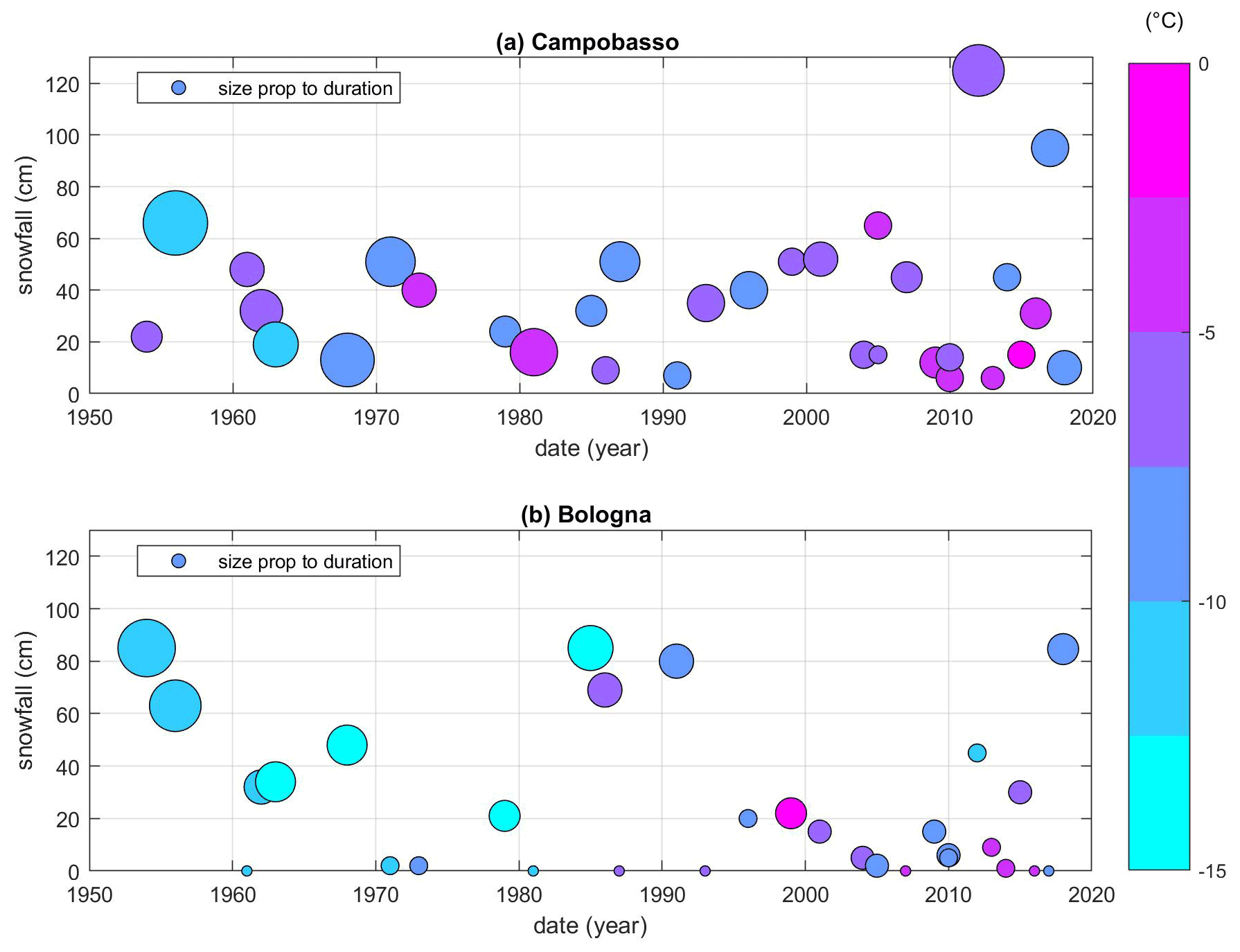
Figure 1 Cold spells from documentary sources. Data recorded in (a) Campobasso (686 m altitude); (b) Bologna (54 m altitude). Each ball represents one cold-spell event. The diameter is proportional to the number of snowfall days. The y axis shows the snowfall measured during each event. The colour shows the minimum near-surface temperature recorded during the event (see “Sources and dataset” section).

The in-depth description of the effects of each cold spell at the country level is presented in Appendix A. Here, we provide a general picture of the typical event through a local analysis focused on the cities of Bologna and Campobasso. The former stands at the southern edge of the Po Valley, at the foot of the north-eastern Apenninic range; the latter is located in the Southern Apennines, at about 45 km from the closest point on the Adriatic coast and 85 km from the closest point on the Tyrrhenian coast. Due to their position, both cities are exposed to snowfall in the case of cold spells characterized by either cold air flowing directly from the east or by Mediterranean cyclogenesis. In the latter case, Arctic air reaches the Mediterranean Sea through the Rhône Valley – often after the formation of a cyclone leeward to the Alps – and hits the eastern Italian coasts as Sirocco and bora winds, as the pressure minimum moves south. In both cases, snowfall in the two cities can be enhanced by the interaction of the easterly low-level winds drawing moisture from the Adriatic with the Apenninic range, due to orographic lift. Data for Bologna are provided by the local Regional Environment Protection Agency (https://www.arpae.it/documenti.asp?parolachiave=sim_annali&cerca=si&idlivello=64, last access: 31 May 2022) and by Randi and Ghiselli (2013), while those used for Campobasso are provided by the Servizio Idrografico e Mareografico di Pescara (https://www.regione.abruzzo.it/content/annali-idrologici, last access: 31 May 2022; http://www.protezionecivile.molise.it/centro-funzionale/la-rete-meteo-idro-pluviometrica.html, last access: 31 May 2022). Figure 1 shows the amount of snowfall, the minimum temperature near the surface and the duration of each cold spell that are recorded in Campobasso and in Bologna between 1954 and 2018 from hydrological archives (https://www.arpae.it/documenti.asp, last access: 31 May 2022).

Given the heterogeneous and, in some cases, unofficial origin of the considered data, we only aim to draw a qualitative picture. Overall, our analysis indicates that extreme snowfalls have occurred in recent years, despite warming temperatures (Fig. 1a). For example, 50 to 60 cm snow depth was measured on the coast at the border between Apulia and Marche during the January 2016 event, and a similar amount was recorded in the Campobasso area. The snowfall amounts do not seem to be affected by decreasing trends, although it can be argued that the duration of the events slightly decreases and the associated minimum temperatures slightly increase. In another study performed using reanalysis and observational data, Faranda (2020) performed yearly block maximum analyses of snowfalls over Europe, showing that contrasting trends appear for extreme snowfalls over Italian regions.

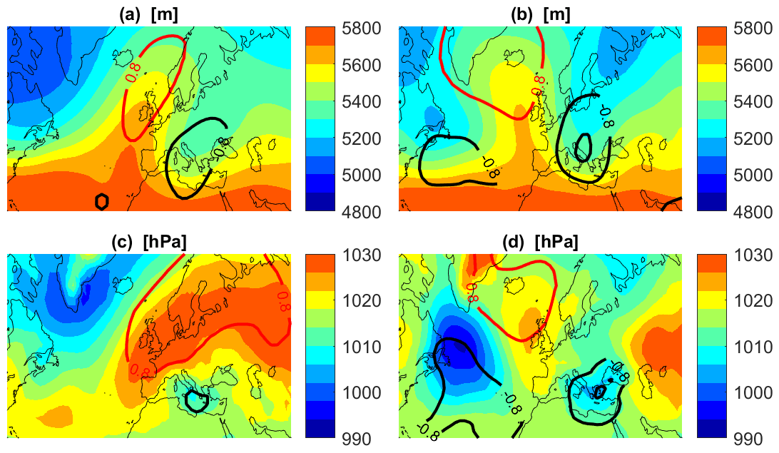
Figure 2 Dynamics for clusters of cold spells over Italy: 500 hPa geopotential height [m] (a, b) and sea-level pressure [hPa] (c, d) averaged over the two clusters of cold spells in Italy found via k means. Cluster 1 (a, c) is characterized by zonally tilted high pressure located between the British Isles and Russia and cluster 2 (b, d) by an omega-blocking pattern between the Atlantic and Europe. Black and red isolines represent negative and positive standardized anomalies.

2.2 Observed cold-spell dynamics

Besides the qualitative analysis involving the cities of Bologna and Campobasso briefly presented in Sect. 2.1, we now aim to characterize the dynamic and thermodynamic features of the considered cold spells at the synoptic scale. To this purpose, we rely on the National Centers for Environmental Prediction (NCEPv2) Reanalysis dataset. In particular, we consider geopotential height at 500 hPa (Z₅₀₀) and sea-level pressure (SLP) as dynamical fingerprints and to compute the analogues (Jézéquel et al., 2018); temperature at 850 hPa (T₈₅₀) to track cold air advection without surface disturbances (Grazzini, 2013); 2 m temperature (T_2 m) to characterize near-surface conditions; and daily precipitation rate (PRP).

Although our analysis is focused on cold spells affecting an area containing Italian borders, the dynamic determinants of such cold spells span much larger scales. For this reason, we consider a larger area, including Europe, European Russia, and the North Atlantic, over a 2.5^∘ grid between [22.5–70^∘ N, 80^∘ W–70^∘ E]. We first perform an unsupervised cluster analysis based on the Z₅₀₀ standardized anomaly fields using a k-means algorithm (Michelangeli et al., 1995), and we inspect the Z₅₀₀, SLP and T₈₅₀ fields averaged over each cluster.

For Z₅₀₀ and SLP, we consider standardized anomalies from the December–January–February–March (DJFM) climatology, since these months include all the events described in Appendix A. Standardized anomalies are obtained by subtracting the DJFM mean and dividing by the DJFM standard deviation.

In order to choose the optimal number of clusters, we first performed a scree plot (not shown), obtained by plotting the within-groups sum of squared differences from the cluster centroids. This analysis did not give clear indications about the ideal number of clusters. Therefore, we compared clustering results at different values of k, finding that for k=3 two of the three clusters displayed very similar spatial features, and with larger k the resulting clusters can always be reduced to two main patterns: we then choose k=2. We remark that the k-means algorithm and other clustering techniques are based on assumptions such as equal size and sphericity of the clusters, which can be met only in coarse approximation in real-world high-dimensional datasets. In particular, the poor indications from the scree plot may be due to the different number of events assigned to each cluster (respectively, 22 and 10 for k=2). However, we find the results consistent enough to allow for a qualitative analysis.

In Fig. 2 we show the Z₅₀₀ fields (Fig. 2a and b) and the SLP fields (Fig. 2e and f) averaged over the events in cluster 1 (Fig. 2a and c) and cluster 2 (Fig. 2b and d), and the corresponding standardized anomalies as red (positive) and black (negative) standardized anomalies. The dynamic configurations in the two clusters differ greatly, suggesting the existence of at least two typical large-scale cold-spell drivers.

Cluster 1 presents a pattern resembling a Scandinavian blocking but with positive SLP anomalies displaced to the south, with an anticyclone stretching in a SW–NE direction rather than elevated along the meridians, and low-pressure values centred over the central Mediterranean, mainly confined below 40^∘ N. The axis of the anticyclone is located at about 50–60^∘ N, so that cold Arctic air is free to flow on its southern edge in a ENE–WSW direction, drawn by the Mediterranean low, after assuming partially continental features while streaming over Russia and eastern Europe. In this situation, cold air easily reaches central southern Italy after increasing its humidity content over the Adriatic Sea. This causes snowy precipitation bands to form slightly offshore of the east Italian coast, which can later be amplified by the orographic effect caused by the Apenninic range, with abundant snowfall even at low altitudes (Stocchi and Davolio, 2017).

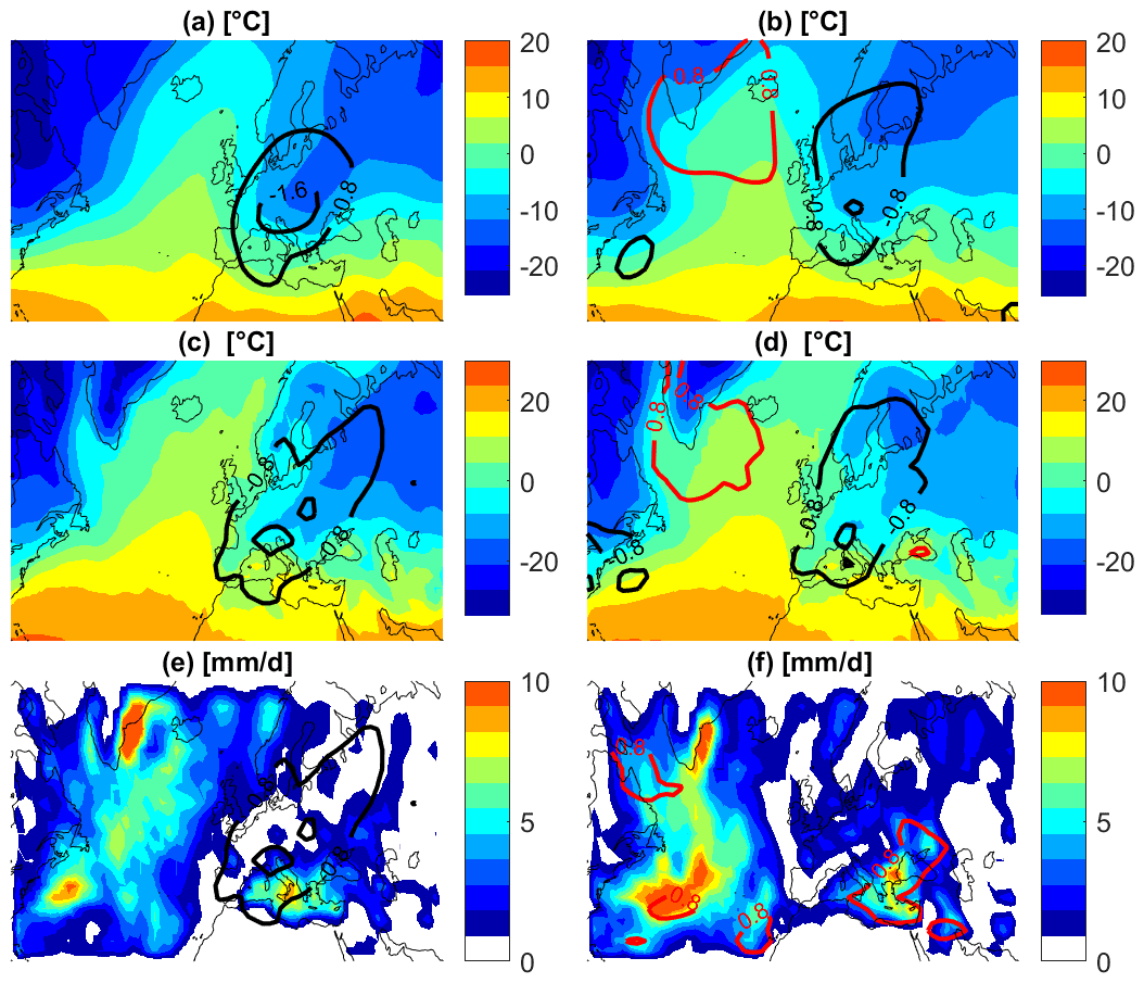
Figure 3 Physics for clusters of cold spells over Italy. Temperature at 850 hPa [^∘C] (a, b), 2 m temperatures [^∘C] (c, d), and precipitation rate [mm d⁻¹] (e, f) averaged over the two clusters of cold spells in Italy found via k means. In cluster 1 (a, c, e) warm air is advected towards the British Isles and cold air flows mainly from Russia and eastern Europe. In cluster 2 (b, d, f) warm air extends north from the Azores to Iceland and cold air flows south from Scandinavia. The temperature field at the surface is very similar, with cold temperatures over continental areas and negative or very low positive daily values over Italy, especially the peninsular regions. Black and red isolines represent negative and positive standardized anomalies.

Cluster 2 is characterized by an Omega wavy structure associated with an Atlantic high-pressure ridge (Falkena et al., 2020; Faranda, 2020) reaching Iceland and with a trough embracing Italy and the Balkans. A trough associated with low Z₅₀₀ values is also present over the North Atlantic, between the Azores and North America. The SLP field presents a similar structure, with a high-pressure system centred over the United Kingdom and a deep low anomaly centred over southern Italy and Greece. In such a situation, cold air is drawn from the north by the Mediterranean cyclone, flowing from Scandinavia over central western Europe and entering the Mediterranean from the Rhône Valley and the Gulf of Trieste due to the presence of the Alps.

Figure 3 shows the corresponding T₈₅₀ (Fig. 3a and b), T_2 m (Fig. 3c and d) and PRP (Fig. 3e and f) fields. We begin with the analyses of T₈₅₀ hPa fields: despite the sensibly different dynamic setting, the penetration of cold air into the Mediterranean is quite similar in the two clusters, with strong negative anomalies embracing the whole central Mediterranean including the entire Italian Peninsula. The main differences concern the UK, Iceland and Scandinavia, due to the different direction of the high-pressure axis. In cluster 1, the tilted high-pressure drives warmer air towards the British Isles and Scandinavia, while the cold anomaly is confined to more southern latitudes. In cluster 2, the meridionally oriented axis brings warmer air towards Greenland and Iceland, while the core of the cold air is located between Scandinavia and central Europe. The T_2 m fields (Fig. 3c and d) generally show above-zero temperatures over central southern Italy during these events: this is partially due to the coarse resolution of the NCEPv2 dataset that regards southern Italy and Sicily as sea grid points. Italy is also a country with a complex geography and mountain ranges (the Alps and the Apennines) extending from the north to the south. This causes a strong temperature gradient across the country. Indeed, for both clusters, the T₈₅₀ temperatures shown in panels Fig. 3a and b are sufficient to produce snowfall in the Po Valley and at low altitudes in the hills and mountains of the country. Finally, the PRP fields (Fig. 3e and f) show that these events are indeed associated with consistent precipitation amounts over southern Italy and Sardinia (especially in cluster 1) and the Balkans (especially in cluster 2).

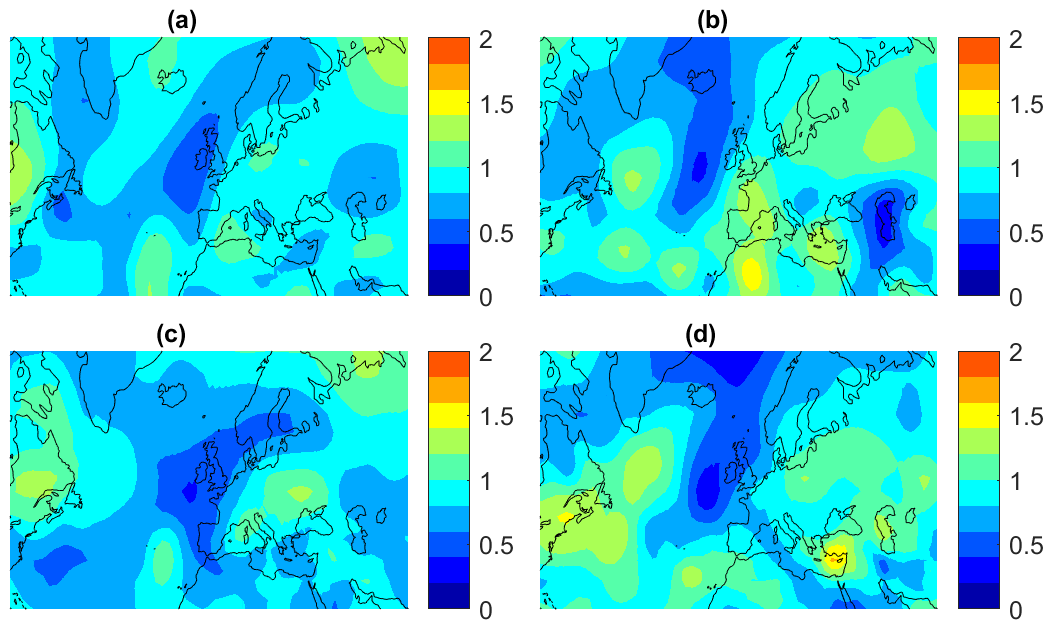
Figure 4 Cluster uncertainty. Standard deviation of 500 hPa geopotential height [m] (a, b) and sea-level pressure [hPa] (e, f) of the two clusters of cold spells in Italy found via k means.

We measure the uncertainty associated with the cluster composites discussed above by computing the standard deviation of the standardized anomalies used for the clustering, shown in Figs. 4 and 5. Low uncertainty is overall associated with the position of Z₅₀₀ maxima and minima driving the cold spells in both clusters. Small values of the SLP standard deviation are also associated with low-level high and low-pressure systems in cluster 1, while the position of the low pressure in the Eastern Mediterranean in cluster 2 is affected by high uncertainty. Concerning temperature, high (cluster 1) and very high (cluster 2) uncertainty is attributed to the position of the western limit of the cold pool of air at 850 hPa (see Fig. 5a and b), and high uncertainty affects the penetration of cold air into the Mediterranean area at the low levels (Fig. 5c and d).

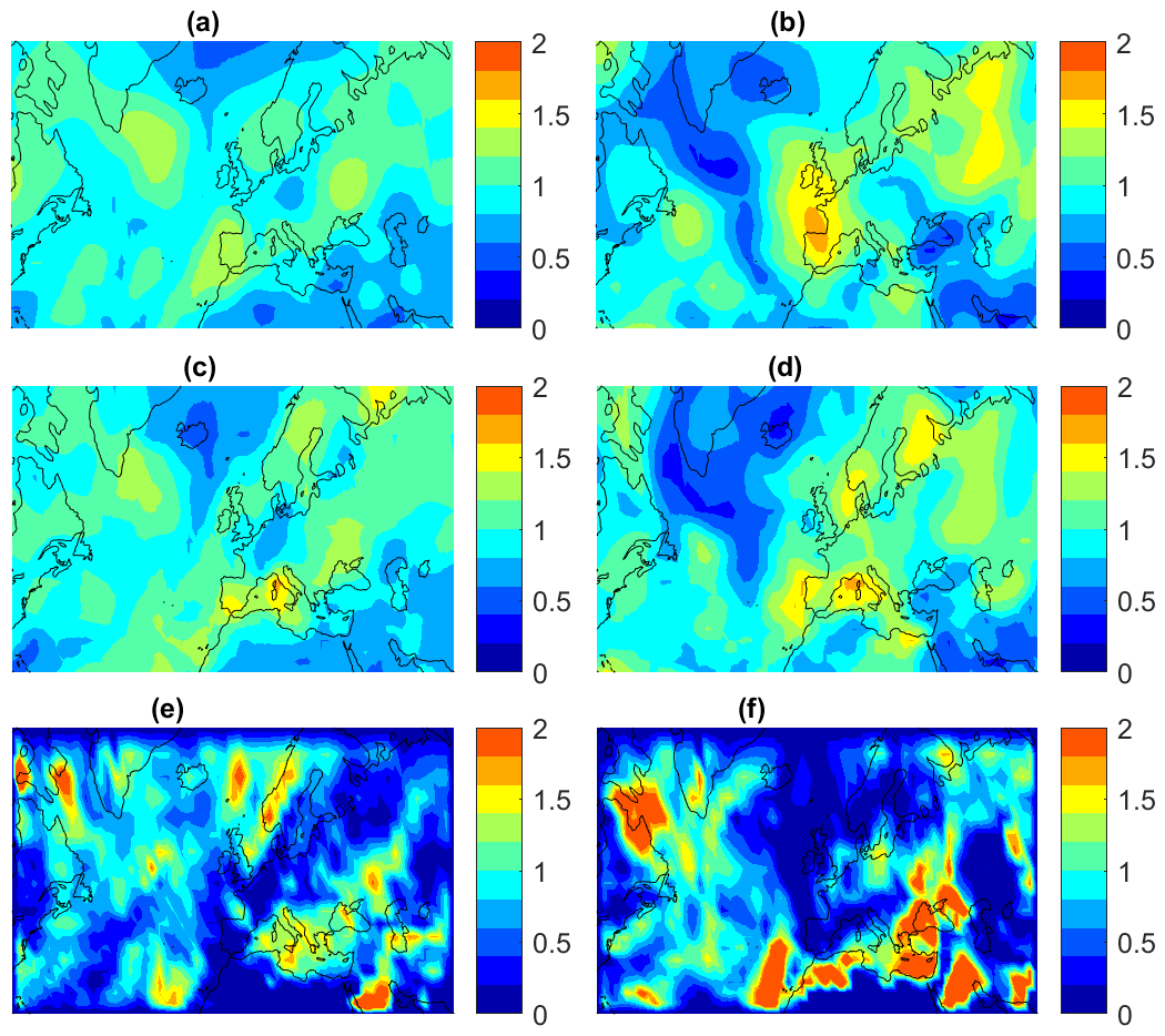
Figure 5 Cluster uncertainty. Standard deviation of temperature at 850 hPa [^∘C] (a, b), 2 m temperatures [^∘C] (c, d) and precipitation rate [mm d⁻¹] (e, f) of the two clusters of cold spells in Italy found via k means.

3 Climate change in atmospheric circulations associated with cold spells in PlaSim

3.1 Model description

In order to understand how the frequency of cold-spell events may change in a warmer climate, we simulate different emission scenarios using PlaSim (Fraedrich et al., 2005a, b), an intermediate-complexity climate model developed at the University of Hamburg and released open source (see https://www.mi.uni-hamburg.de/en/arbeitsgruppen/theoretische-meteorologie/modelle/plasim.html, last access: 31 May 2022). PlaSim has been applied to a variety of problems including climate response theory (Lucarini et al., 2014), storm tracks (Fraedrich et al., 2005b), climatic tipping points (Boschi et al., 2013; Lucarini et al., 2010a), the analysis of the global energy and entropy budget (Fraedrich and Lunkeit, 2008; Lucarini et al., 2010b), the simulation of extreme European heatwaves (Ragone et al., 2018), and the investigation of the late Permian climate (Roscher et al., 2011). The reason of using PlaSim with respect to higher complexity GCMs is the ability to generate long stationary simulations, for which we compute reliable analogues. The horizontal resolution used in this study is about 300 km (T₄₂, $\sim \mathrm{2.8}{}^{\circ }\times \mathrm{2.8}{}^{\circ }$) with 10 vertical, non-equidistant levels. The dynamical core for the atmosphere is adopted from the Portable University Model of the Atmosphere (PUMA). The model includes a full set of parameterizations of physical processes such as those relevant for describing radiative transfer, cloud formation and turbulent transport across the boundary layer. The horizontal heat transport in the ocean can be prescribed or parameterized by horizontal diffusion. The parameterization by horizontal diffusion includes a simplified representation of the large-scale oceanic heat transport, and then it ameliorates the realism of the resulting climate. The atmospheric dynamical processes are modelled using the primitive equations formulated for vorticity, divergence, temperature and the logarithm of surface pressure. The governing equations are solved using a spectral transform method. In the vertical dimension, 10 non-equally spaced sigma (pressure divided by surface pressure) levels are used. The model is forced by diurnal and annual cycles.

3.2 Experimental set-up: the simulation ensemble

In this study we consider four simulations performed with T₄₂ resolution at daily frequency, 450 years long, with a mixed layer ocean. To get a reasonable response and present-day climate, one needs to add an oceanic heat transport in the mixed layer model (slab ocean, without motion). This can be done in several ways: for our set-up, we tuned horizontal diffusion (h_diff) to have a reasonable global mean sea surface temperature (SST) and a realistic response of SST and ice to the forcing ($h_{\mathrm{diff}}=\mathrm{4}\times {\mathrm{10}}^{\mathrm{4}}$).

The first simulation is the control run (hereinafter CTRL) with radiative forcing levels representative of the recent past climate: equivalent CO₂ concentration, including the net effect of all anthropogenic gases, is set to a value of 360 ppmv. Three more simulation runs were produced, based on three of the representative concentration pathways (RCPs) developed for the climate modelling community as a basis for long-term and near-term modelling experiments (Van Vuuren et al., 2011). We consider the RCP-2.6, RCP-4.5 and RCP-8.5 scenarios (Van Vuuren et al., 2011), which consist of raising the radiative forcing from 2005 to 2100, to reach an increase of, respectively, 2.6, 4.5 and 8.5 W m⁻² compared to pre-industrial conditions. In our simulations (denoted RCP2.6, RCP4.5 and RCP8.5), the equivalent CO₂ concentration is set at the beginning to be, respectively, 490, 660 and to 1470 ppm and kept constant afterwards. These correspond to the end-of-century equivalent CO₂ concentrations of the respective RCPs. By using these three different forcing scenarios, we are able to explore climates ranging from moderate warming to no climate policy.

This way, we explore three scenarios where excess heat is stored in the atmosphere in different amounts, and we investigate which differences in the dynamics associated with cold and snowy spells in the present climate appear, if any. We will analyse the Z₅₀₀, SLP, T₈₅₀ and T_2 m fields corresponding to the PlaSim event analogues to the cold-spell clusters to characterize their dynamical and thermodynamical fingerprints, by analogy with the discussion presented in Sect. 2.2. Moreover, we will consider daily precipitation to check whether similar dynamics are still associated, under different RCPs, with precipitation patterns similar to the ones found in the present climate.

3.2.1 Bias correction

Climate models, even those with higher complexity than PlaSim, are characterized by a finite resolution, thus leaving smaller scales unresolved, and contain several physical and mathematical simplifications that make climate simulations computationally feasible, while also introducing a certain level of approximation. This results in statistical biases that can be easily observed when comparing control runs to observations or reanalysis datasets. In order to mitigate the effects of these biases, a bias correction step can be performed. Bias correction usually consists of adjusting specific statistical properties of the simulated climate variables to a validated reference dataset in the historical period. The target statistics can be very simple, such as a central tendency index like the mean (Shrestha et al., 2017), or it may include dynamical features, such as a certain number of autocorrelation function lag or spectral density frequencies for time series data (Nguyen et al., 2016). It can aim to correct the entire probability distribution of the observable. The correction can also be carried out in the frequency domain, so that the entire time dependence structure is preserved. For an overview of various bias correction (BC) methodologies applied to climate models, see, for example, Teutschbein and Seibert (2012, 2013) and Maraun (2016).

Given the lower complexity and the relatively coarse grid of PlaSim compared to other regional or global circulation models, we rely on simple methodologies. We apply BC only to the T₈₅₀, T_2 m and PRP, since we will use their composites to characterize the phenomena associated with the dynamic analogues of the two clusters. No BC is usually performed on Z₅₀₀ and SLP; moreover, the analogue search is based on standardized anomalies, making BC unnecessary for these variables.

For the variables characterized by approximately symmetric distributions (T₈₅₀ and T_2 m), we adopt a simple linear scaling bias correction (Shrestha et al., 2017), which consists of constraining the CTRL mean of each variable to match the NCEP values and applying the same transformation to the RCP simulations.

For PRP, we must rely on a different method, given the strong asymmetry characterizing the distribution of precipitation. We choose quantile mapping based on regularly spaced quantiles, with a wet-day correction to obtain an equal fraction of days with precipitation in the reference and corrected data: the empirical probability of nonzero precipitation is found, and the corresponding modelled value is selected as a threshold. All modelled values below this threshold are set to zero. This technique is described by Gudmundsson et al. (2012) and implemented in the fitQmapQUANT function from the R package qmap.

3.3 Analogue detection

We base our analysis of cold spells in PlaSim on the search for dynamic analogues (Yiou et al., 2013) in a similar way to in Faranda et al. (2020). This way of defining analogues by embedding the extreme events of interest in the climate simulation is rooted in the link between dynamical systems and extreme value theory (Lucarini et al., 2012), and the events selected as analogues are linked to quantities such as the local attractor dimension and the persistence of the dynamical system state (Pons et al., 2020). Here we briefly sketch the methodology, redirecting the reader to the aforementioned papers.

Let X_t denote the value of a gridded variable of interest (here, the Z₅₀₀ anomaly field) at time t=1, …, T. Let ζ represent the same variable in correspondence of one event of interest, in our case one of the Z₅₀₀ anomaly fields associated with the two clusters obtained as described in Sect. 2.2 and shown in Fig. 2c and d. We compute the metric

$$g_t=-\ln \left\{\mathrm{dist}\left(X_t,\mathit{\zeta }\right)\right\},$$

where dist(,) denotes a distance function, in our case the Euclidean distance. The choice of the Euclidean distance has been motivated in Yiou et al. (2013) and in Faranda et al. (2017) for the computation of dynamical indicators such as the local attractor dimension. Furthermore, the minus sign allows us to interpret the g_t function as an indicator of the proximity of analogues.

Now let g_c be a high percentile of the distribution of g, for example corresponding to the probability $P(g_t\ge g_c)=\mathrm{0.98}$: the events satisfying this condition are considered analogues of ζ. As already mentioned, we limit our analysis to the extended winter season DJFM, as these months include all the 32 selected cold-spell events.

The procedure is carried out, for each cluster, according to the following steps:

1. define ζ as the Z₅₀₀ standardized anomaly field corresponding to cluster i=1, 2 and X_t as the ensemble of all the NCEP Z₅₀₀ standardized anomaly fields;

2. compute the metric $g_{t,\mathrm{NCEP}}^{Z_{\mathrm{500}}}$ using data selected in step 1;

3. determine the critical value $g_c^{Z_{\mathrm{500}}}$ such that $P(g_{t,\mathrm{NCEP}}^{Z_{\mathrm{500}}}\le g_c^{Z_{\mathrm{500}}})=p^{*}$;

4. now take PlaSim Z₅₀₀ fields as X_t, while keeping the same reference field ζ;

5. compute the metrics $g_{t,r}^{Z_{\mathrm{500}}}$ using Z₅₀₀ from PlaSim runs, with r = CTRL, RCP2.6, RCP4.5, RCP8.5;

6. estimate probabilities ${\mathit{\pi }}_{i,r}=P(g_{t,r}^{Z_{\mathrm{500}}}\le g_c^{Z_{\mathrm{500}}})$ and compare them to the reference value p^*;

7. regard all events satisfying $g_{t,r}^{Z_{\mathrm{500}}}\ge g_c^{Z_{\mathrm{500}}}$ as cold-spell analogues.

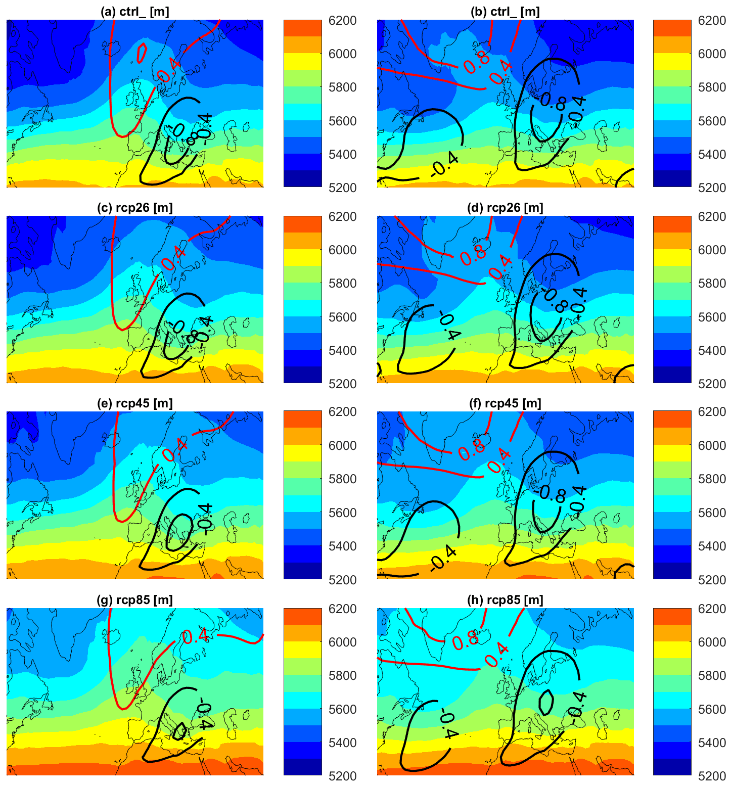
Figure 6 The figure shows the 500 hPa geopotential heights in PlaSim simulations: average of the 500 hPa geopotential height [m] for cluster 1 (a, c, e, g) and cluster 2 (b, d, f, h) of analogues. (a, b) Control run. (c, d) RCP2.6 run. (e, f) RCP4.5 run. (g, h) RCP8.5 run. Isolines represent positive (in red) and negative (in black) standardized anomalies.

Steps 1–3 select the ($\mathrm{1}-p^{*}$) fraction of the closest winter analogues of the two main configurations leading to the selected cold spells. Steps 4–6 allow us to determine whether the frequency of the configuration is significantly different in the PlaSim scenarios compared to NCEP and, if so, in which direction. This way, we can establish if climate change can affect atmospheric dynamics, leading to an atmosphere more or less conducive to synoptic configurations that can result in a cold spell. In step 7 we then select the analogues of the configurations of interest in the PlaSim runs. This way, we can study the composites of other variables of interest, namely temperature and precipitation, to assess the phenomena associated with the same dynamics under different climate scenarios. In our analysis, we choose $p^{*}=\mathrm{0.98}$, so that we regard the 2 % NCEP Z₅₀₀ anomaly fields closest to the cluster fields as analogues.

3.4 Results

Our first result follows from the estimation of the probabilities described in step 6. in the previous paragraph. These are the probabilities π_i,r that the Z₅₀₀ field at date t from run r is an analogue of the centroid of cluster i=1, 2 as close as the ($\mathrm{1}-p^{*}$) % of the closest NCEP Z₅₀₀ fields. In particular, we are interested in the differences $\mathrm{\Delta }{p}_{i,r}=({\mathit{\pi }}_{i,r}-p^{*})$. If $\mathrm{\Delta }{p}_{i,r}>\mathrm{0}$, the configuration is more extreme and less frequent than in historical climate. By contrast, values $\mathrm{\Delta }{p}_{i,r}<\mathrm{0}$ indicate a more recurring event. The percentage change in frequency of events that are cold-spell dynamic analogues can be obtained as $-\mathrm{\Delta }{p}_{i,r}/(\mathrm{1}-p^{*})$.

The results of this analysis are summarized in Table 1.

Table 1 Change in frequency of cold-spell analogues for each of the considered events, divided by cluster. The values corresponding to the RCPs are adjusted by subtracting the values relative to the CTRL run, which quantify PlaSim's bias in analogues frequency; unadjusted values are shown in parentheses.

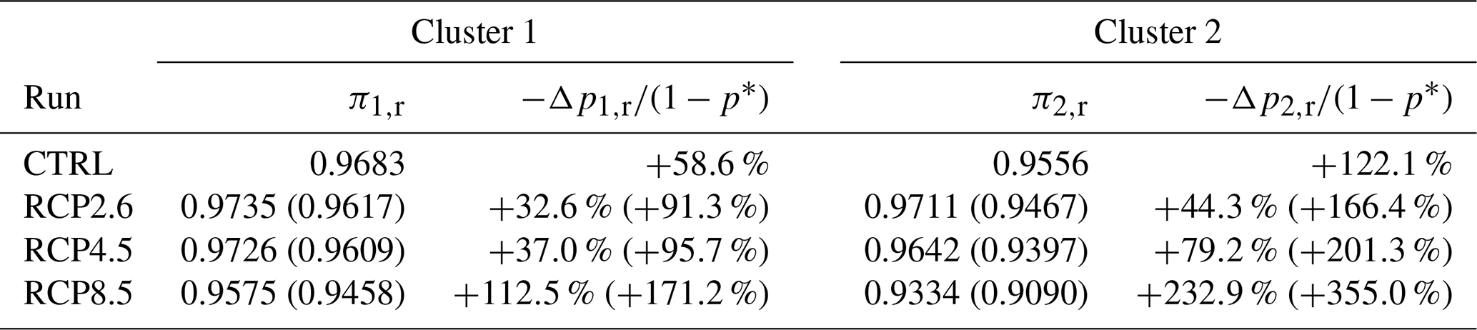
The results for the CTRL run inform us about the capability of PlaSim to reproduce the frequency of the two dynamical fingerprints of cold spells associated with the two clusters of events. Both configurations are much more frequent in PlaSim than in NCEPv2, with a +58.6 % frequency of the circulation associated with the cluster 1 centroid and +122.1 % for cluster 2. We offset the results for the RCP scenarios by subtracting these frequency biases; unadjusted results are shown in parentheses.

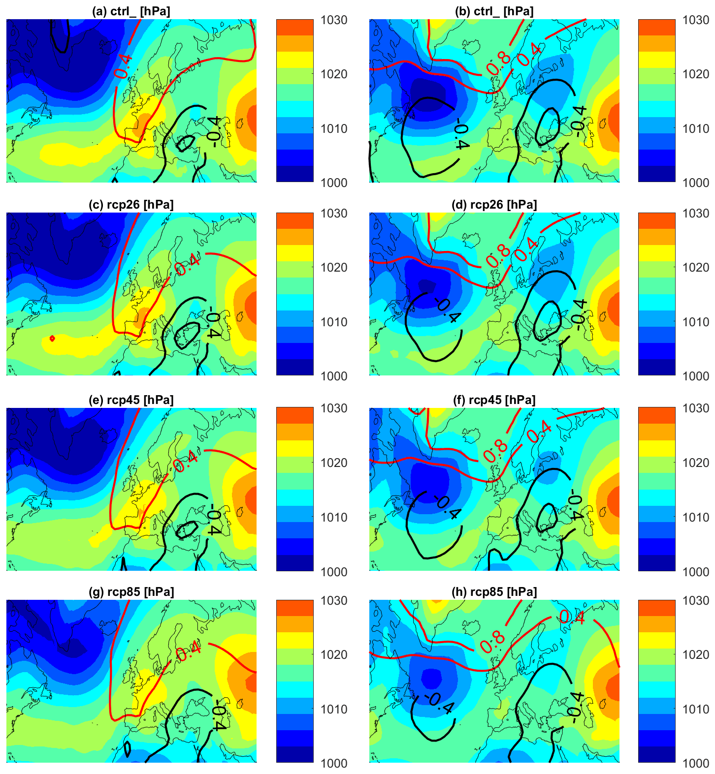
Figure 7 Sea-level pressure in PlaSim simulations: average of the sea-level pressure [hPa] for cluster 1 (a, c, e, g) and cluster 2 (b, d, f, h) of analogues. (a, b) Control run. (c, d) RCP2.6 run. (e, f) RCP4.5 run. (g, h) RCP8.5 run. Isolines represent positive (in red) and negative (in black) standardized anomalies.

Both configurations become increasingly more frequent with growing radiative forcing. It is worth mentioning that this analysis does not discriminate between an increased number of Atlantic ridge and Scandinavian blocking episodes and their longer persistence, both of which may lead to more analogues. Nevertheless, these result clearly suggest a higher number of days characterized by configurations leading to a flow of Arctic air towards the Mediterranean area under climate change.

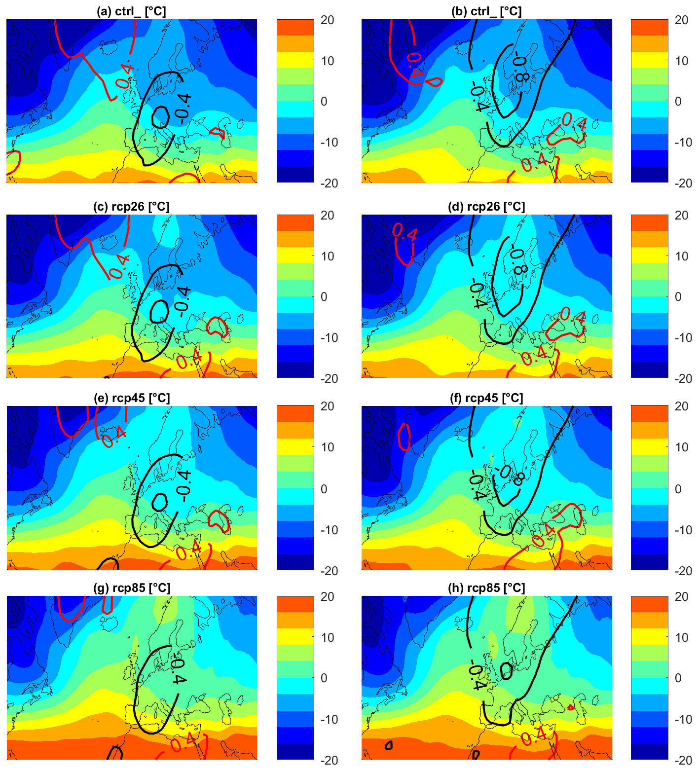
Figure 8 The figure shows 850 hPa temperature in PlaSim simulations: average of the 850 hPa temperature [^∘C] for cluster 1 (a, c, e, g) and cluster 2 (b, d, f, h) of analogues. (a, b) Control run. (c ,d) RCP2.6 run. (e, f) RCP4.5 run. (g, h) RCP8.5 run. Isolines represent positive (in red) and negative (in black) standardized anomalies.

Figure 6 shows the composites of Z₅₀₀ analogues fields in the CTRL (Fig. 6a and b) and RCP (Fig. 6c–h) runs for analogues of cluster 1 (Fig. 6a, c, e and g) and cluster 2 (Fig. 6b, d, f and h), found with the rule shown in step 7 of the procedure described above. Given that ${\mathit{\pi }}_{i,r}<p^{*}$ in all cases, these analogues are less than the ($\mathrm{1}-p^{*}$ %) of the days in each run; however, given that each PlaSim run is 450 years long, they are more in absolute number. The isolines show the corresponding positive (in red) and negative (in black) standardized anomalies, on which we base the analogue search. The Z₅₀₀ fields are associated with the SLP fields shown in Fig. 7. Whereas the anomaly patterns overall resemble those of the NCEP reanalysis for both Z₅₀₀ and SLP, we observe that, when increasing the equivalent CO₂ concentration, the magnitude of the negative anomalies in the Mediterranean area decreases, especially in RCP8.5.

Figure 8 show the composites of the T₈₅₀ fields. As expected, with growing radiative forcing, negative temperatures are confined progressively more to the north and east, with only an isolated cold patch still persisting over Russia under RCP8.5. A similar behaviour is also observed for T_2 m, shown in Fig. 9. We remark that, in the RCP2.6 simulation, T₈₅₀ and T_2 m values are still low enough to be associated with snow precipitation in most of the hills and mountain areas of Italy.

The precipitation patterns associated with these analogues are shown in Fig. 10. The distribution of precipitation in the CTRL run is fairly similar to those of NCEP cluster 2 for both clusters, showing the most abundant precipitation over the central eastern Mediterranean Sea including most of Italy, the Balkans, Greece, Turkey and the Black Sea; a lack of precipitation is observed in southern Italy and Sardinia for analogues of cluster 1.

In summary, in a warmer climate, the frequency of dynamic configurations leading to Z₅₀₀ fields similar to the geopotential maps in Fig. 2 may even increase dramatically, depending on the scenario. Clearly, this does not imply that Italy would paradoxically experience increasing snowfalls in the RCP climates. Indeed, the PlaSim simulations display a clear increase in temperature that would make snowfall overall much less likely, at least at low altitudes.

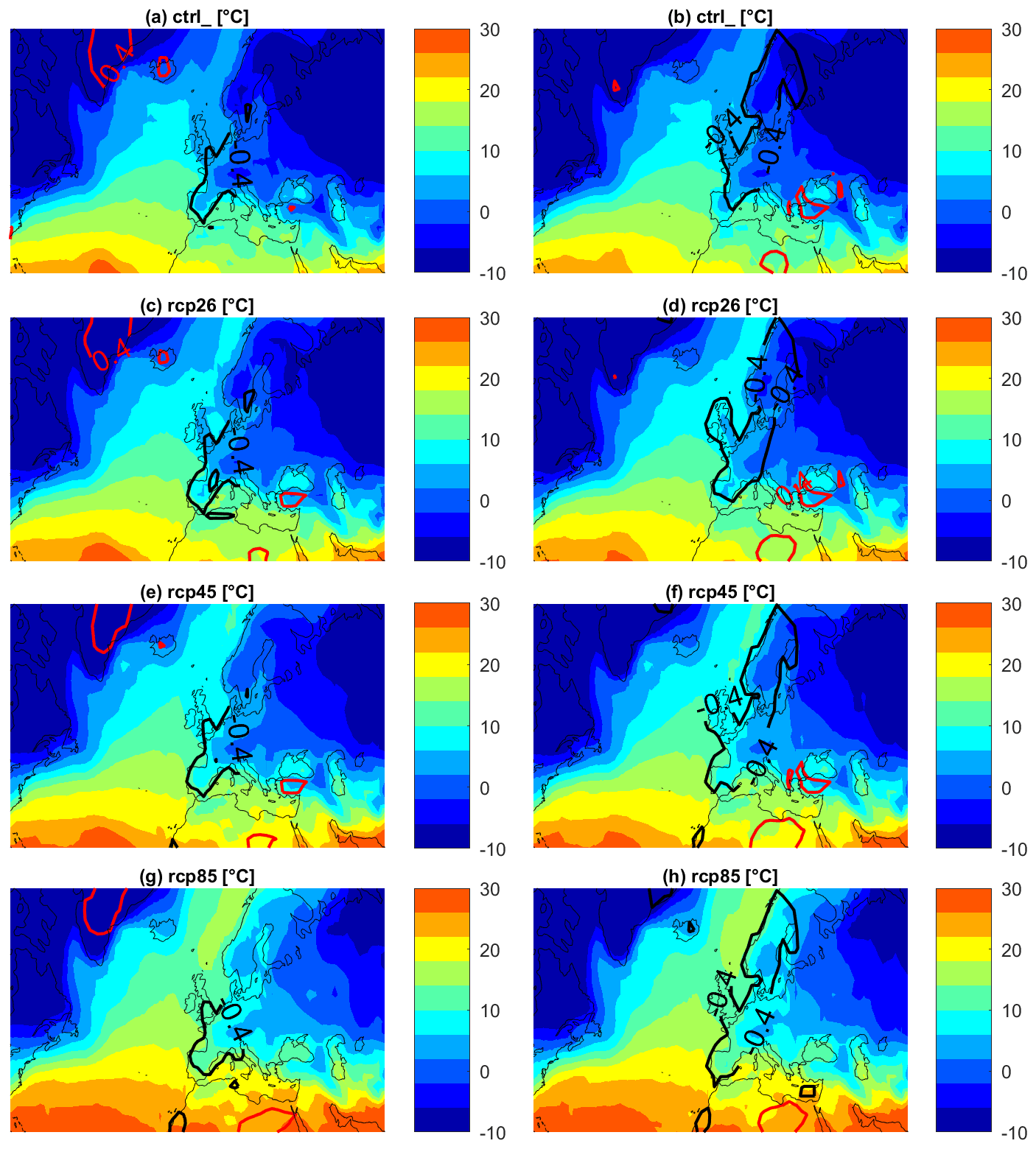
Figure 9 The figure shows 2 m temperatures in PlaSim simulations: average of the 2 m temperature [^∘C] for cluster 1 (a, c, e, g) and cluster 2 (b, d, f, h) of analogues. (a, b) Control run. (c, d) RCP2.6 run. (e, f) RCP4.5 run. (g, h) RCP8.5 run. Isolines represent positive (in red) and negative (in black) standardized anomalies.

Figures B1–B5 show the root mean squared deviation (RMSD) of the analogues of each cluster from the corresponding cluster centroid. Compared to the within-cluster standard deviations shown in Figs. 4 and 5, higher uncertainty is associated with the position of the high- and low-level cyclones and anticyclones among the analogues, particularly for the SLP minimum in cluster 1. Moreover, very high uncertainty is associated with the negative anomalies of both T₈₅₀ and T_2 m, suggesting that the composites in Figs. 8 and 9 encompass configurations leading to very different thermodynamic set-ups. Similar or slightly lower uncertainty than in NCEP is, instead, associated with the area characterized by precipitation in the Mediterranean area.

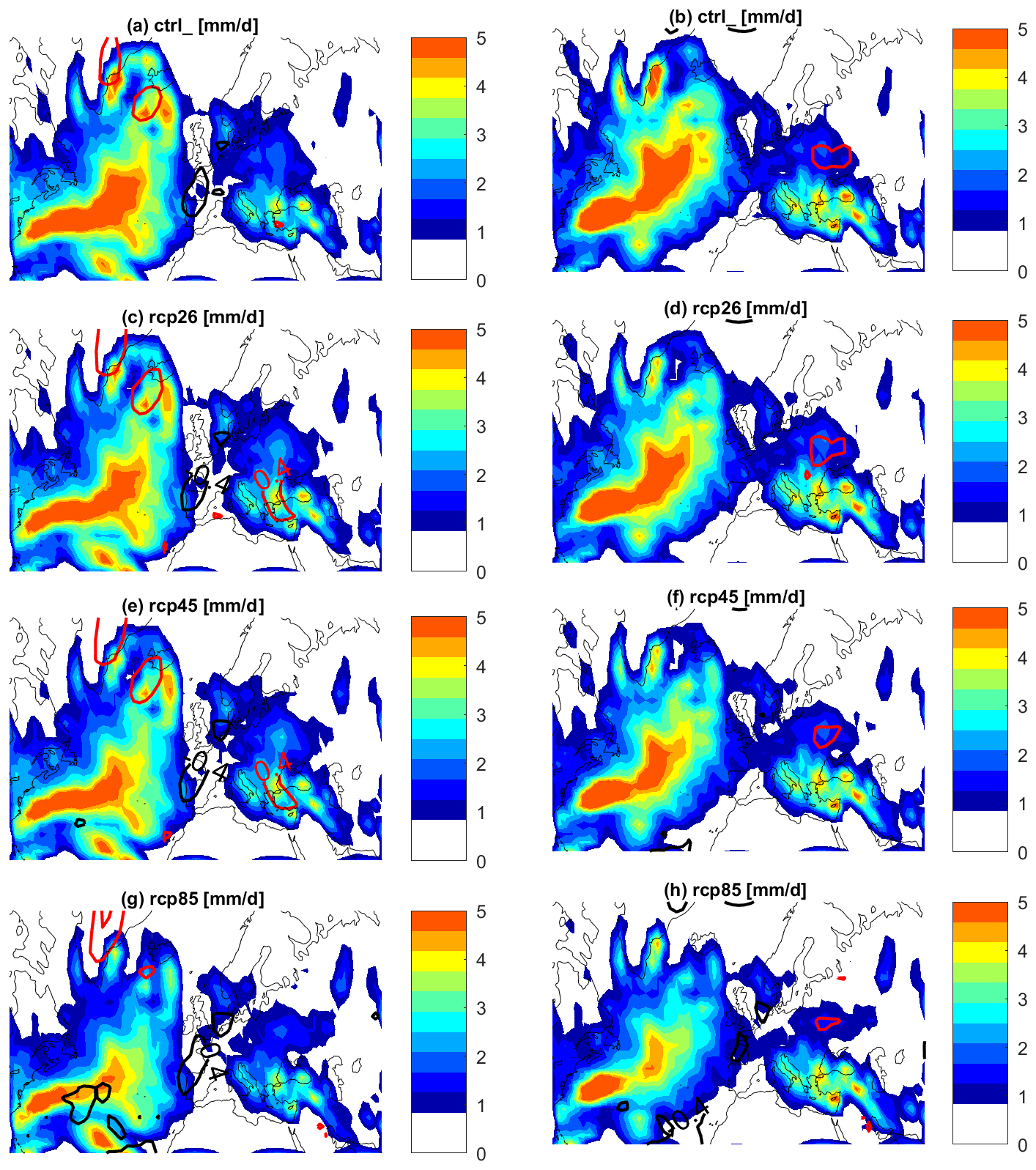
Figure 10 Daily precipitation rates in PlaSim simulations: average of the daily precipitation rates [mm d⁻¹] for cluster 1 (a, c, e, g) and cluster 2 (b, d, f, h) of analogues. (a, b) Control run. (c, d) RCP2.6 run. (e, f) RCP4.5 run. (g, h) RCP8.5 run. Isolines represent positive (in red) and negative (in black) standardized anomalies.

4 Discussion and conclusion

We have characterized high-impact cold spells that affected Italy in the course of the past 68 years by assessing their common dynamical large-scale signature. Despite the differences in duration, snowfall and temperature recorded during each event, the corresponding Z₅₀₀ fields can be grouped according to two main dynamic fingerprints. Both are characterized by the presence of a low-pressure area over the central Mediterranean, associated with an anticyclone either zonally tilted between western Europe and Russia, with pressure maxima over central Europe (cluster 1), or elevated over western Europe (cluster 2). In both cases, cold air is drawn towards Italy by the Mediterranean low-pressure area, flowing mainly from Russia (cluster 1) or Scandinavia (cluster 2).

Then, after assessing the capability of PlaSim to reproduce dynamic analogues of these events in the CTRL run, we studied the influence of climate change on the frequency of such analogues using three steady-state increased emission scenarios. The PlaSim control run showed a tendency to overestimate the frequency of both configurations. All three RCP runs are associated with more frequent configurations potentially leading to cold spells, with frequency increasing with equivalent CO₂ concentration and a precipitation pattern that does not change substantially over the Mediterranean region. This increased frequency of Atlantic ridge and Scandinavian-like blocking patterns could be associated with a wealth of phenomena driven by mean anthropogenic climate change but still debated in the current scientific literature, such as the Arctic amplification or the increased land–sea temperature contrast (Cohen et al., 2020; Hamouda et al., 2021). Arguments to the contrary show an increase in flow zonality over the North Atlantic but mostly for the autumn (de Vries et al., 2013) and the summer seasons (Fabiano et al., 2021).

Since temperatures are projected to be contextually higher, cold spells and snow are naturally expected to decrease overall, especially under RCP4.5 and RCP8.5; however, we argue that the formation of cold air over the Arctic winter would not be completely suppressed, hence making cold-spell events still possible, and they remain relatively likely under the mitigated RCP2.6 scenario. This observation is particularly important, as RCP2.6 is representative of the current target to comply with the requirements of the Paris Agreement (Arias et al., 2021).

Moreover, the temperature fields shown in Figs. 8 and 9 are obtained by averaging over a large number of events, but temperatures low enough to generate snowfall will still be possible in single events. Considering the increased likelihood of the associated dynamical configuration, this is an important message, as the disruptive effects of these events may be exacerbated by lower attention and preparedness in much warmer climates.

This study comes with some caveats and limitations: although we have validated the behaviour of PlaSim against the NCEP reanalysis, results for frequency changes for cold spells crucially depend on the position and the destabilization of the jet stream. It is known that different climate models have a different response of jet stream dynamics to climate change (Arctic amplification (Cohen et al., 2014) or zonation (Francis and Vavrus, 2012)).

The use of an intermediate-complexity model like PlaSim allowed us to evaluate climate change in atmospheric dynamics associated with cold spells in a steady, much warmer climate, showing how the frequency and intensity of cold spells may decrease less than expected, due to a higher likelihood of synoptic configuration favourable for cold air to flow towards the Mediterranean.

Appendix A: Description of detected events

In this section, we describe each extreme cold event selected as a cold spell in this study. The mains characteristics of the events are the occurrence of snowfalls in regions where snow cover has usually been rare or absent for a long time (e.g. lowlands and coasts), large socioeconomic impacts (e.g. in 2017), extreme minimum temperatures and extreme amount of snowfalls. The date reported at the beginning of each event is the one selected as the most representative day of each cold-spell event, and it is the one used for the analogue search. The information about the duration of the events is reported in the text for each description.

1. 4 January 1954: a cold spell rapidly built up in the Mediterranean in January 1954 (an exceptional month in Spain). Heavy snowfalls affected all of northern Italy, including lowland areas in the Po Valley. In 24 h, up to 60 cm of snow fell over Turin, Brescia, Milan, Piacenza, Cremona, Reggio Emilia, Bologna and Vicenza according to information found in the press (Resto del Carlino, 1954).

2. 4 February 1956: one of the coldest and snowiest events of the 20th century in Europe. On 2 February, the −15 ^∘C isotherm at 850 hPa was located above the Po Valley (wetterzentrale.de, 2022); snow storms affected the entire country, with historical snowfall in Rome. A powerful extratropical cyclone embedded in a very cold mid-tropospheric air core struck the southern regions causing heavy snowfalls in Rome and throughout central and southern Italy, with blizzards and heavy frost. Significant snowfall was even reported on the Sicilian coast: in Palermo, the minimum temperature dropped to 0 ^∘C (Servizio Idrografico del Ministero dei Lavori Pubblici, 1956), and the city was blanketed by several centimetres of snow, which also fell on the southern coasts of Sicily and the island of Lampedusa (Corriere del Mezzogiorno, 2011).

3. 17 December 1961: December was a very cold month for most of Italy with historical snowfall in southern Italy coastal areas, with up to 30 cm accumulation in Bari (Pacucci, 2022). After 3 d of heavy snowfall, a record snow height of 370 cm was reported in Roccacaramanico (1050 m a.s.l. – above sea level – on the east side of the Central Apennines) on 20 December (Genio Civile di Pescara, 1961), and all the Adriatic regions were affected by heavy snowfalls (meteogiornale.it, 2022e).

4. 31 January 1962: Sicily reported several historical records of daily low temperature as in Lentini (−2.5 ^∘C), Caltanissetta (−4.5 ^∘C), Caltagirone (−3.2 ^∘C) and Castronovo di Sicilia – Lago Pian del Leone (−8.5 ^∘C) (Servizio Idrografico del Ministero dei Lavori Pubblici, 1962). Heavy snowfall occurred on the north coast, in Palermo and Capo d'Orlando (meteolive.it, 2022a).

5. 22 January 1963: the winter of 1963 was one of the coldest in western European records. Sea frost trapped Norway's islanders, while a record low temperature of −41.2 ^∘C was recorded in the northern Swedish village of Karesuando. Average temperatures for the month were in excess of −5 ^∘C below normal from southern England across Europe to the Urals. Warsaw reported an average temperature of −12.4 ^∘C for January, while Paris averaged −5.5 ^∘C below normal. Mediterranean regions averaged about −3 ^∘C below normal (James, 1963). The upper reaches of the Thames River froze (thamesweb.co.uk, 2022), and the lowest temperature in Germany was measured on 2 January at Quedlinburg at −30.2 ^∘C (Eichler, 1971). In Italy the temperature drop was brought on by strong bora winds of up to 110 km h⁻¹ (Ufficio Idrografico del Po, 1963), and snow accumulation over Friuli Venezia Giulia (5 to 10 cm) reached Venice, where the lagoon also froze. Very low temperatures (Trieste: −9 ^∘C; Udine: −10 ^∘C: Pordenone: −15 ^∘C; Milan: −8 ^∘C; Bologna: −7 ^∘C; Ufficio Idrografico del Po, 1963) affected all other regions of Italy, with snowstorms over Tuscany, Marche, Abruzzo, Molise and Apulia, and several cities were completely isolated (meteogiornale.it, 2022f; Randi and Ghiselli, 2013).

6. 12 January 1968: between 9 and 15 January 1968, Tuscany and nearby areas were affected by one of the strongest cold spells on record for the region. Extreme daily low temperatures were recorded: Città di Castello (Umbria, 295 m), −23 ^∘C; Arezzo (S. Fabiano) (277 m) −14.2 ^∘C; Verghereto (812 m) −15.2 ^∘C; Cortona (393 m) −8.7 ^∘C (Genio Civile di Pisa, 1968; Ufficio Idrografico di Roma, 1968). Heavy snowfall affected the area, with snow depth measuring: 65 cm in Eremo di Camaldoli (1111 m a.s.l.), 60 cm in Verghereto (812 m a.s.l.), 15 cm in Arezzo (S. Fabiano, 277 m a.s.l.) and 19 cm in Florence (Ximenian Observatory, 51 m a.s.l.) (Genio Civile di Pisa, 1968; La Nazione, 1968).

7. 28 February 1971: on 24 February, the presence of an omega blocking with an anticyclone meridionally elevated towards the British Isles and a trough with a pressure minimum over the central Mediterranean, triggered a flow of Arctic air towards the Mediterranean. After affecting northern Europe, the cold spell reached Italy, causing a severe temperature drop between 28 February and 1 March. On the morning of 1 March, almost all of Italy recorded minimum temperatures below zero even in lowland and coastal areas: −5 ^∘C in Florence and Pisa (Genio Civile di Pisa, 1971), −4 ^∘C in Ardea, near Rome (Ufficio Idrografico di Roma, 1971), and −1 ^∘C in Naples (Genio Civile di Napoli, 1971) with snowfall that also reached the coastal areas of the city (La Stampa, 1971).

8. 1 December 1973: at the beginning of December, a cold air mass associated with a low-pressure area reached Italy from Scandinavia, with the −15 ^∘C isotherm located over the Alps. Cold conditions persisted for a long time, yielding to low minimum temperatures during the first 2 weeks of December, reaching −7 ^∘C in Novara, Treviso and Arezzo, −6 ^∘C in Udine and Potenza, −5 ^∘C in Foggia, −2 ^∘C in Trieste, and −19 ^∘C on Monte Cimone (2173 m a.s.l.), where a north-easterly wind with 133 km h⁻¹ was also recorded. Due to these conditions, highways remained closed in Tuscany for half a day, disrupting important road networks. Snow fell in Florence, (17 cm), and Valle del Serchio received 30 cm of snow, after around 40 years during which snow was almost absent. Snow accumulations (≈15 cm) were also recorded in Perugia, Gubbio, Assisi, Spoleto and Sangemini (sienanews.it, 2022; Ufficio Idrografico del Magistrato delle Acque di Venezia, 1973; Genio Civile di Pisa, 1973; Genio Civile di Catanzaro, 1973; Genio Civile di Bari, 1973; Ufficio Idrografico del Po, 1973; Aeronautica Militare, 2022)).
   

9. 15 January 1979: a large pool of Arctic air stretching up to the North African coasts brought a cold spell that affected most of Europe, causing several fatalities. The cold air caused wind storms in the Tyrrhenian Sea, followed by a severe temperature drop. Snowfall occurred in Tuscany, Sardinia, and most of central and southern Italy, with snowstorms in the Marche, Abruzzo, Molise and Basilicata regions. The most abundant snowfalls were observed on 19 January with the advection of more temperate and humid air from the south-west. Traffic problems due to frost on the roads and to iced pipes were reported (Resto del Carlino, 1979a, b).

10. 8 January 1981: a very cold air mass penetrated deeply into the central Mediterranean Sea, accompanied by an intense storm over the south of Italy. On 8 January, western central Sicily was disrupted by unprecedented amounts of snow for the area, with 30 cm of snowfall even on the coasts. Extremely unusual snowfall was observed even on Pantelleria, a small island located south of Sicily, with only 5 m elevation above sea level. Some cities in the provinces of Palermo, Trapani, Messina and Enna remained isolated for days. The temperature reached a historical minimum of −0.5 ^∘C in Palermo, where continuous snow precipitation for more than 24 h is an exceptional event (La Repubblica, 2009a; meteolive.it, 2022a; Genio Civile di Palermo, 1981).

11. 7 January 1985: from 1 to 17 January 1985, Italy and most of western Europe were affected by a disruptive and persistent cold spell. A cyclogenesis over central Italy, between Tuscany and Lazio, triggered strong bora winds and historical snowfalls that affected Florence with 40 cm of accumulation (up to 80 cm in Val di Cecina) and Rome with 30 cm. The pressure minimum moved towards the south-east between 6 and 9 January, and the snow also reached Campania and the rest of the south with accumulations of up to 25 cm in the hilly zones of Naples, which had not happened since 1956 (Genio Civile di Napoli, 1985). Between 1 and 11 January minimum-temperature records were broken in Florence (Peretola, −23.2 ^∘C) and Piacenza (S. Damiano, −22.2 ^∘C). The northern regions were particularly affected a few days later, between 14 and 17 January: temperatures of around −20 ^∘C were registered in the Po Valley, and exceptional snowfalls disrupted traffic and industrial activities in the cities of the north, including Milan, with historical accumulations (valdarnopost.it, 2022; Il Mattino, 2018; La Stampa, 1985).

12. 24 December 1986: Christmas Day 1986 was characterized by strong winds and 850 hPa isotherms of −10 ^∘C that covered most of the Italian Peninsula (wetterzentrale.de, 2022). In Pescara, on the evening of 26 December, the temperature reached −9 ^∘C and about 15 cm of snow fell. Snowfall affected the entire Adriatic side of the country (5 cm in Perugia, more than 30 cm in Molise). In Ancona (Falconara) wind gusts exceeded 95 km h⁻¹ with a minimum temperature of −6 ^∘C. The snow then reached Sardinia and even Apulia, where the temperature in Bari dropped to −1 ^∘C (Genio Civile di Bari, 1986). A record low temperature for December was measured in Pantelleria, with 2.6 ^∘C on 25 December (Genio Civile di Palermo, 1986).

13. 3 March 1987: cold air and stormy weather reached the extreme south-east of Italy, with a peak on 8 March 1987 when the −12 ^∘C 850 hPa isotherm covered the whole of Apulia (Genio Civile di Bari, 1987). Snow fell in the southern cities of Naples, Crotone and even in Palermo. Impressive snow accumulations were recorded on those days: in Gioia del Colle snowfall reached 72 cm, with permanent snow on the ground for a total of 9 d, exceptional for the area (Genio Civile di Bari, 1987; 3bmeteo.com, 2022d; La Repubblica, 1987; meteogiornale.it, 2022g).

14. 31 January 1991: cold air entered the Mediterranean as strong bora winds, causing temperature to drop to −4.2 ^∘C in Trieste (Ufficio Idrografico e Mareografico di Venezia, 1991). Snow fell in Bologna, Rimini, Forlì and eventually in the Marche coastal area, with 5 cm of accumulation in the harbour city of Ancona. The cold air mass also spread west over the Po Valley, from Veneto to Piedmont, with widespread snowfalls. Minimum temperatures of −21.2 ^∘C were recorded at Passo Rolle, −12 ^∘C in Novara and −11.6 ^∘C in Bologna. The 7 February is one of the coldest (Ufficio Idrografico e Mareografico di Venezia, 1991; Ufficio Idrografico e Mareografico di Parma, 1991) days in the history of northern and central Italian climatology (Randi and Ghiselli, 2013; meteoservice.net, 2022; La Repubblica, 1991)).

15. 1 January 1993: a zonally tilted anticyclone with pressure maxima between the UK and Scandinavia drew a large Arctic air patch from Russia towards Italy. Due to the peculiar configuration, cold air flowed from Russia through Ukraine, Romania and the Balkans and then mostly affected southern and central Italian regions, especially the Adriatic side, where the snow fell also in coastal areas. The absolute minimum temperature record was broken in Bari (−5.9 ^∘C) (Aeronautica Militare, 2022). Snow fell in the southern part of the Italian Peninsula and Sicily (Reggio Calabria and Messina) but also in the Po Valley (Parma, Modena, Reggio Emilia), on the Adriatic coast, from Rimini to Cattolica, and in Tuscany. Snowfall was also observed in the northern part of the Rome metropolitan area. Snowfall affected the Tyrrhenian and Adriatic sides of Italy simultaneously, which is rare. The cold air moving westward then caused additional extensive snowfalls in the north and central Italy. Intense cold conditions persisted for a long time in the Po Valley with record-breaking temperatures, such as −13 ^∘C in Milan and almost −20 ^∘C in Emilia (meteolive.it, 2022c; Corriere della Sera, 1993).

16. 27 December 1996: this cold spell also affected the UK and France (−7 ^∘C in Paris; Le Parisien, 1997) causing the Thames River to freeze in London and 200 fatalities (Jordan-Bychkov and Murphy, 2008). On 27 December snow storms struck the north and the Adriatic side of Italy from Romagna to the south. On 29 December, heavy snowfall affected central Italy and southern Tuscany in unusual areas (20 cm were recorded on the Lazio coast, 35 cm in Porto Santo Stefano; Aeronautica Militare, 2022). On 30 December snow fell again over the north in Milan, Como, Varese, Pavia and throughout the whole of Piedmont. A snow storm blew in the coastal city of Genoa. Extremely low minimum temperatures affected the areas covered by snow (between −10 and −15 ^∘C in southern Tuscany and Umbria; Ufficio Idrografico e Mareografico di Pisa, 1996). The official weather station of the city of Arezzo (Molin Bianco, 248 m a.s.l.) recorded a minimum of −15 ^∘C on 30 December (Aeronautica Militare, 2022), a monthly record for December since the beginning of records (1957). (La Repubblica, 1996; meteolive.it, 2022c).

17. 31 January 1999: Arctic air reached Italy, particularly affecting the central and northern regions, on 5 February. The snow affected the entire Po Valley, from Venice to Turin, with accumulations of up to 30 cm on the plain. Snow also fell abundantly in the coastal cities of Rimini, Ancona, Grosseto and Genoa and in the Tuscan cities of Florence and Lucca. A snowstorm struck Viterbo and snowflakes were also observed in Rome with a remarkable temperature of −6 ^∘C (Ufficio Idrografico e Mareografico di Roma, 1999), which caused the public city fountains to freeze, a rather unusual and damaging phenomenon, given the often ancient origin of the fountains. The temperatures decreased sharply, and there were a few ice days (i.e. days with maximum temperatures below zero) in the city. Other notably low temperatures include −0.2 ^∘C in Palermo on 31 January (Osservatorio Astronomico G.S.Vaiana, 1999), −12 ^∘C in Norcia (Ufficio Idrografico e Mareografico di Roma, 1999) and −21 ^∘C in Dobbiaco (1213 m altitude; Aeronautica Militare, 2022). Strong bora winds affected Trieste on 4 February. Snow fell on the Sicilian coasts and accumulated up to 5–10 cm in a few hours on the beaches of the Nebrodi area (Arpa Regione Emilia Romagna, 1999; La Repubblica, 1999; meteoweb.eu, 2022a).

18. 8 December 2001: before affecting northern Italy, cold air reached parts of central eastern Europe from Russia. On the evening of 13 December, the air mass entered the Po Valley in the form of a strong bora wind, causing convection accompanied by a blizzard-like snowfall that caused transport, electricity and phone line disruptions, and isolated several small towns in northern Italy. In Trieste the bora wind blew at 116 km h⁻¹ and −4 ^∘C. In Tarvisio on 15 December the temperature reached −16 ^∘C (Arpa Friuli Venezia Giulia, 2020). This storm is today remembered as the famous “Blizzard of Saint Lucia”, long remembered by the inhabitants of the north, since the blizzard combined heavy snowfalls with damaging winds. On that occasion, the origin of cold air masses was eastern Europe and Russia. Due to the strong wind, snow fell horizontally and stuck to the walls of buildings, rails and guardrails of highways with heavy transport disruptions and several accidents. The snow accumulation fluctuated between 5 and 25 cm on the plains, depending on the area and on exposure to wind, with larger values in Emilia-Romagna: temperatures of −16 ^∘C were recorded in Fiorenzuola (422 m altitude), −7 ^∘C in Reggio Emilia and −5 ^∘C in Cesena on 17 and 18 December (La Repubblica, 2001; meteoweb.eu, 2022b).

19. 20 January 2004: during this event, icy currents flowed from the north-east towards northern Italy, with weak snowfalls over Emilia, up to medium–low altitudes. In the following days, however, it snowed again in the north and in the central regions at lower altitudes: snow reached Tuscany and Lazio, with snowflakes even in Rome. The temperatures in these days of January were particularly low in the north-eastern Alps and in central and southern Italy, where markedly negative values were recorded over the usually mild Tyrrhenian plains (−5.2 ^∘C at Fiumicino, −6.3 ^∘C in Rome and −4 ^∘C in Ciampino; Protezione Civile del Lazio, 2004). The whole region of Lazio experienced particularly cold days. The cold also affected Irpinia and Basilicata with temperatures below zero on the Ionian sea coast, Molise, Abruzzo and Apulia, where the snow occasionally fell also on the coast. During this event, exceptionally low temperatures were measured in these areas: the temperature dropped to zero in Foggia, a coastal town in Apulia, (Ufficio Idrografico e Mareografico di Bari, 2004) and the coastal cities of Naples, Lamezia Terme and Catania. Low daily maximum temperatures (below the 10 ^∘C degrees) were recorded also on the Sicilian Tyrrhenian coast, from Messina to Trapani, and even in the Syracuse area (Autorità di Bacino del Distretto Idrografico della Sicilia, 2004).

20. 22 January 2005: western and central Europe experienced below average temperatures throughout the winter, with the cold peaking during the month of January. In northern Italy snow fell abundantly: in Lombardy snow height reached 30 cm, with peaks of up to 40–45 cm, and even the coastal city of Genoa suffered snowfalls (Arpa Liguria, 2005; Aeronautica Militare, 2022). Snow fell also over Marche, Abruzzo, Campania and Basilicata, where inland areas were affected by snowfalls for several days, and accumulations exceeded 1 m in Abruzzo as well as in some areas of Irpinia. There were road disruptions as car drivers were trapped in the snow on highways. Stormy weather also affected other European countries, particularly France and Spain. In France four avalanches detached from the mountains in Savoy caused many victims in ski resorts (meteogiornale.it, 2022b; Corriere della Sera, 2005).

21. 2 March 2005: a cold and snowy spell hit central and southern Italy. Snow fell in the hills of Naples, at medium–low altitude in Calabria, and with abundant accumulations on the central Adriatic coast (from southern Marche to Molise). A few days later, snowfall spread to the north and Tuscany (Servizio Idrologico Regionale Regione Toscana, 2020). Up to 30 cm of snow fell in Liguria (Arpa Liguria, 2005), in Milan and in most of Lombardy, on the plains of Emilia, in Piedmont, and in the north of Tuscany; it snowed in Veneto, turning Verona, Venice and Rovigo white (meteogiornale.it, 2022c). On 1 March 2005, the lowest temperatures of the winter were recorded, with a country average of −0.5 ^∘C, which entered Italy's climatic history. The temperatures in the Alps region reached peaks of −23 ^∘C (Marcesina record of −34 ^∘C; Veneto, 2022), −20 ^∘C at Cimone in the Apennines, −16 ^∘C at Terminillo (Protezione Civile del Lazio, 2005) and −10.8 ^∘C in L'Aquila (Ufficio Idrografico e Mareografico di Pescara, 2005). Among lowland cities, we mention −12 ^∘C in Piacenza, −11 ^∘C in Novara, −10.4 ^∘C in Udine (Arpa Friuli Venezia Giulia, 2020) and −9 ^∘C in Arezzo (Servizio Idrologico Regionale Regione Toscana, 2020).

22. 13 December 2007: the peculiarity of this cold spell was the exceptional occurrence of abundant snowfalls, blizzard conditions and an extreme low in temperatures over most of the Sardinian territory, at altitudes on average above 400 m. Also noteworthy are the 2 m of snow accumulated over an altitude of 1000 m on the slopes of Mount Limbara. Towns were largely unprepared to manage the event. An electricity blackout affected Cagliari for several hours, and schools remained closed for 2 d. Disruptions were reported in road connections: the main road of the Sardinian network of state highways suffered numerous blocks due to some trucks blocking the roads. In Nuoro, the snowfall exceeded 50 cm, breaking the record (Regione Sardegna, 2007). A strong wind and rough seas were observed on the coasts. Low temperatures also affected central and southern Italy: −10 ^∘C and icy roads were reported in Calabria, and snowfalls in Molise as well as in the hinterland of Bari, Foggia and Taranto (Ufficio Idrografico e Mareografico di Bari, 2007), and in Basilicata (Agenzia Regionale Protezione Civile della Basilicata, 2007); below-zero temperatures were recorded on the Ionian coast (La Repubblica, 2007; meteolive.it, 2022b).

23. 17 December 2009: most of central and northern Europe was struck by this cold spell. On 19 December, snow fell over most of northern Italy, and it was especially copious in Tuscany (Servizio Idrologico Regionale Regione Toscana, 2020). A strong glazed frost occurred in Emilia and Liguria (3bmeteo.com, 2022b). Extreme low temperatures were recorded in some lowland locations (especially on 20 December) in Friuli Venezia Giulia (Arpa Friuli Venezia Giulia, 2020): Udine Rivolto −18 ^∘C, Pordenone −12.4 ^∘C, Cervignano del Friuli −17.3 ^∘C, in coastal locations such as Lignano −6.3 ^∘C, in some Alpine valleys such as Tarvisio (754 m a.s.l.) −18.3 ^∘C and Fusine (850 m a.s.l.) −22 ^∘C (La Repubblica, 2009b; Il Quotidiano, 19/12/2009; meteogiornale.it, 2022d).

24. 12 February 2010: snowfalls affected several regions, from Emilia-Romagna to Calabria, Marche and Sardinia (Regione Sardegna, 2010). Bologna airport was closed for several hours: 17 flights were cancelled and 15 diverted. The heaviest snowfall in Rome (Agenzia Regionale per lo Sviluppo e l'Innovazione dell'Agricoltura del Lazio, 2020) since February 1986 was recorded, causing transport disruptions, with many roads closed both within and outside the city. Many interventions were required to rescue motorists involved in collisions and stuck on the highway between Marche and Romagna (the distribution of comfort items for at least 2000 people stuck in cars was necessary). A blizzard hit the Sila region, where schools were closed for a few days (https://www.roma-artigiana.it/, last access: 31 May 2022; La Stampa, 2010; La Repubblica, 2010).

25. 11 December 2010: an Arctic air mass reached the eastern side of Italy, giving rise to intense snowfalls on the Adriatic and Tyrrhenian coasts (especially the coasts surrounding the city of Livorno). Snow also turned Tuscany (25 cm fell in Florence), Umbria and part of Lazio white, with snowflakes observed in Rome. An exceptional snowstorm hit Ancona and the surrounding areas between 14 and 15 December. There, the Adriatic-effect snow contributed to reaching snow heights of up to 30 cm in the Chieti area and 40 cm in Lanciano. The temperatures were extremely cold over most of Italy. Milan Malpensa airport measured a minimum temperature of −14 ^∘C and Rome reached −7.7 ^∘C, a record value for the month of December (Agenzia Regionale per lo Sviluppo e l'Innovazione dell'Agricoltura del Lazio, 2020). Very low temperatures were also recorded on 17 December in Forlì (−6 ^∘C) and in Parma (−7.5 ^∘C; Arpae.it, 2020) as well as in Ancona (-6.8 ^∘C), in Florence (−7.3 ^∘C ), in Isernia (−11.8 ^∘C) and in Salerno (−7.2 ^∘C) (Centro Funzionale Multirischi per la Meteorologia, l'Idrologia e la Sismologia Regione Marche, 2010; Servizio Idrologico Regionale Regione Toscana, 2020; Centro Funzionale Multirischi Regione Campania, 2010; Il Messaggero, 2010; 3bmeteo.com, 2022c; Randi and Ghiselli, 2013).

26. 2 February 2012: the February 2012 cold spell affected a large part of Europe and spread down to North Africa in the period between 27 January and 20 February 2012, causing over 650 deaths in the areas concerned. The event was characterized by extremely low temperatures, especially over eastern Europe, with an absolute minimum of −42.7 ^∘C in Finland and heavy snowfall in the remaining European countries (assessment of the observed extreme conditions during late boreal winter 2011/12; WMO, 2013). On 4 February, snow even fell in Algiers with an accumulation of about 20 cm, and the cold air even brought snow to Tunisia (ansamed.info, 2022). In Italy the cold spell caused serious hardship, and there were at least 57 victims (La Repubblica, 2012). From the end of January, a stream of Arctic air reached the peninsula. At first, only the northern regions were affected (e.g. Alessandria recorded −20 ^∘C, Milan −14.5 ^∘C), but the cold later spread to the central and southern regions. Snow fell in most of Italy, especially in Emilia-Romagna and in the provinces of Pesaro and Urbino, Ancona, Macerata and Fermo in the central regions. A daily low of −7.6 ^∘C was recorded in Bologna on 6 February, −10.2 ^∘C in Parma and −6.2 ^∘C in Rimini, (Arpae.it, 2020). Snow fell over several areas of southern Italy, such as Basilicata and Calabria, and on Monte Pellegrino in Palermo on 14 February (Agenzia Regionale Protezione Civile della Basilicata, 2012; palermotoday.it, 2022).

27. 7 February 2013: this cold spell consisted of a polar trough spreading towards the Mediterranean region: the −12 ^∘C 850 hPa isotherm reached central Europe and a 850 hPa temperature of −6.7 ^∘C was measured at midnight on 10 February in the Milan Linate airport radiosounding (meteonetwork.it, 2022). The minimum temperatures of 10 February were very cold in the lower Ticino Valley, and 11 February was a snowy day on most of the northern Italian plains, with diurnal temperatures of around 0 ^∘C. This was an important snow event on the Po Valley: 20 cm accumulated in Milan during 36 h of snowfall, and the largest accumulations were found in the Brianza area north of Milan, where peaks exceeding 35 cm were recorded (Centro Meteorologico Lombardo, 2022). Heavy snowfalls were reported in Emilia, in the Lombardy plain, Veneto, lower Trentino and Friuli. Accumulations reached up to 10–15 cm snow height between Emilia, southern Veneto and southern Lombardy. Stormy weather also affected the rest of Italy, but snow fell only at mountainous altitudes, with some episodes at lower altitudes especially in Tuscany (Arpae.it, 2020; Veneto, 2020; Servizio Idrologico Regionale Regione Toscana, 2020; milanotoday.it, 2022; La Repubblica Milano, 2013).

28. 28 December 2014: this cold spell affected the south of Italy with locally exceptional snowfalls, especially in Sicily and Apulia, the latter recording important accumulations on the plains and coasts. Snow also appeared in Naples and on the Amalfi coast. Snowfalls affected Sicilian coasts including the city of Messina, the hills and the hinterland of Palermo, with large accumulations, and Syracuse. The event was modest in Catania, with accumulations only in the hills of the city. The extreme south-eastern tip of Sicily experienced snowfall on New Year's Eve, an extremely rare event, as these southernmost areas of the country had not received snow since January 1905. Historic snowfall were also recorded in Pachino, a city famous for the production of a special type of cherry tomatoes. Snowfall also affected Sicilian towns on the Ionian side, like Avola and Noto. This cold spell was extraordinary also in the south of Sardinia, where Cagliari and surrounding areas were covered by snow (La Repubblica, 2014; meteoweb.eu, 2014).

29. 5 February 2015: Italy was affected by stormy and snowy conditions. It snowed extensively in Piedmont as well as in Liguria, a region also affected by strong winds. Snow fell at low altitudes and in the lowlands in the northern Italy and in part of central Italy. During this event, due to the strong winds, Sicily was isolated and the connections with the smaller islands were interrupted. In the surroundings of Etna, snow, wind gusts and ice caused blizzard conditions. In Enna the temperature dropped to −4.2 ^∘C (Autorità di Bacino del Distretto Idrografico della Sicilia, 2015). The most difficult situation was observed in Ustica, as ferries could not reach the island for 12 d, and essential medicines were delivered in dangerous operations by helicopters. Many flights were cancelled at Sicilian airports. Many roads and highways remained closed as the snow cover exceeded 50 cm in some areas. On 9 February, ANAS (Azienda nazionale autonoma delle strade) reported that heavy snowfall causing traffic jams in the provinces of L'Aquila and Teramo. In northern Italy, snow caused an electrical blackout: numerous municipalities in the Bologna area, and many others in the region, experienced outages in light, heating and water supply as well as malfunctions in the telephone network and the internet. On 7 February a big snowfall involved the city of Parma and the whole Emilia-Romagna region (−7.4 ^∘C on 9 February; Arpae.it, 2020), with road accidents and problems with the supply of electricity for about 12 000 customers in the municipality of Parma (livesicilia.it, 2022; today.it, 2022; La Repubblica Bologna, 2015).

30. 16 January 2016: on 17 January cold air flowed from Russia, passed over the barrier of the Alps and reached the Apennine chain. Due to the strong winds and rough sea, the Aeolian Islands were isolated and the highest peaks of the islands (Stromboli and Salina) were covered in white. Storm surges struck the Sicilian north coast (Autorità di Bacino del Distretto Idrografico della Sicilia, 2016). In Molise, snow covered almost the entire region, even at low altitudes. The city centre of Lanciano (ansa.it, 2022) was covered by up to 25 cm of snow, and 50 to 60 cm snow height was also measured in those parts bordering the coast. Snow fell throughout Basilicata (Agenzia Regionale Protezione Civile della Basilicata, 2016) and temperatures reached −8 ^∘C. White peaks appeared at lower altitudes as well as in the Aspromonte. Accumulations reached up to 20 cm in some area of Cosenza (150 m a.s.l.) and over 30 cm in the highest hills surrounding the city. Snow caused many issues, mainly to traffic circulation with traffic jams on the Salerno–Reggio Calabria highway. Calabria was the area most affected by the snow, even recording some casualties (meteopalermo.it, 2022; La Repubblica, 2016).

31. 5 January 2017: from 5 to 21 January 2017, a cold spell affected most of eastern and central Europe and part of southern Europe, causing the death of at least 60 people. The cold and snowfalls mainly affected central and southern Italy. The regions most affected by this cold spell were the Adriatic ones, namely Marche, Abruzzo, Molise, Apulia and Basilicata. Snow reached almost all coastal areas of these regions, with snow totals of up to 40 cm. On 8 January, the beach of Porto Cesareo in Apulia was covered at some point with accumulations of 22–23 cm, resulting as the third most snowy Italian beach since 2000. The situation was worse in inland areas, where snow often exceeded 2 m height. A strong snowstorm affected the entire Marsicano sector (Abruzzo), with temperatures ranging between −10 and −13 ^∘C and final accumulations of almost 1 m and temperatures below −10 ^∘C below 1300 m altitude (Regione Abruzzo, Servizio Presidi Tecnici di Supporto al Settore Agricolo, 2017). On 9 January, the combination of heavy snowfall and a seismic swarm in central Italy triggered a disastrous avalanche that hit the town of Rigopiano in Abruzzo: a landslide swept away and destroyed a hotel, causing the death of several people that had been stranded there due to the exceptional snowfall, which also considerably complicated rescue operations in this region (Corriere della Sera, 2017; Aljazeera, 07/01/2017; severe weather.eu, 2022; La Repubblica, 2017).

32. 18 February 2018: the cold spell affected Europe between the end of February 2018 and the beginning of March. The major anomalies concerned the central and northern sector of Europe with temperatures between 5 and 9 ^∘C below the reference average of 1971–2000, but consistent anomalies were, however, also recorded over Italy. The cold was felt more intensely in central and northern Italy and marginally in the far south of Italy and in Sicily. In the northern regions, temperature values were up to 8–9 ^∘C below seasonal averages. Rome experienced moderate snowfall (3–4 cm of snow), which caused temporary disruptions in ground transport. The last snowfall in Rome, in chronological order, was February 2012, when the city was covered with snow for the first time after many years. In Cagliari, the mistral (north-westerly) wind was extremely strong, with gusts of up to 100 km h⁻¹, creating disruptions in the maritime connections between Sardinia and the rest of the continent. Gale force winds were recorded in all regions; for example wind exceeded 70 km h⁻ in Capo Caccia, on the north coast, and 80 km h⁻¹ in Capo Carbonara, on the south coast (Aeronautica Militare, 2022). Snow covered the slopes of the Riviera di Ponente and fell in Rome, Naples (the last snow event was in 1956), Olbia and Bari (nimbus.it, 2022). The minimum temperatures of 27–28 February were the lowest in the last 20–30 years above 1500 m at many locations in the Alps, with up to −25 ^∘C recorded at 2500 m. A second pulse of cold air mass reached Italy through the Karst Plateau in the early hours of 25 February, spreading throughout northern Italy during the daytime, along with winds and irregular snowfalls on the plains between Emilia-Romagna and Piedmont. New monthly records for February were observed in Bologna (−9.1 ^∘C), in Rome-Ciampino (−6.2 ^∘C; second lowest after the −6.5 ^∘C reached on 2 March 1963) and −1.1 ^∘C in Brindisi (Aeronautica Militare, 2022; Il Foglio, 2017; La Gazzetta di Parma, 2018; La Gazzetta del Serchio, 2018; nimbus.it, 2022).

Appendix B: Analogue variability around cluster centroids

Figure B1 The figure shows 500 hPa geopotential height uncertainty in PlaSim analogues: root mean squared difference in standardized 500 hPa geopotential height (standard deviations) between analogues and cluster centroids for cluster 1 (a, c, e, g) and cluster 2 (b, d, f, h). (a, b) Control run. (c, d) RCP2.6 run. (e, f) RCP4.5 run. (g, h) RCP8.5 run.

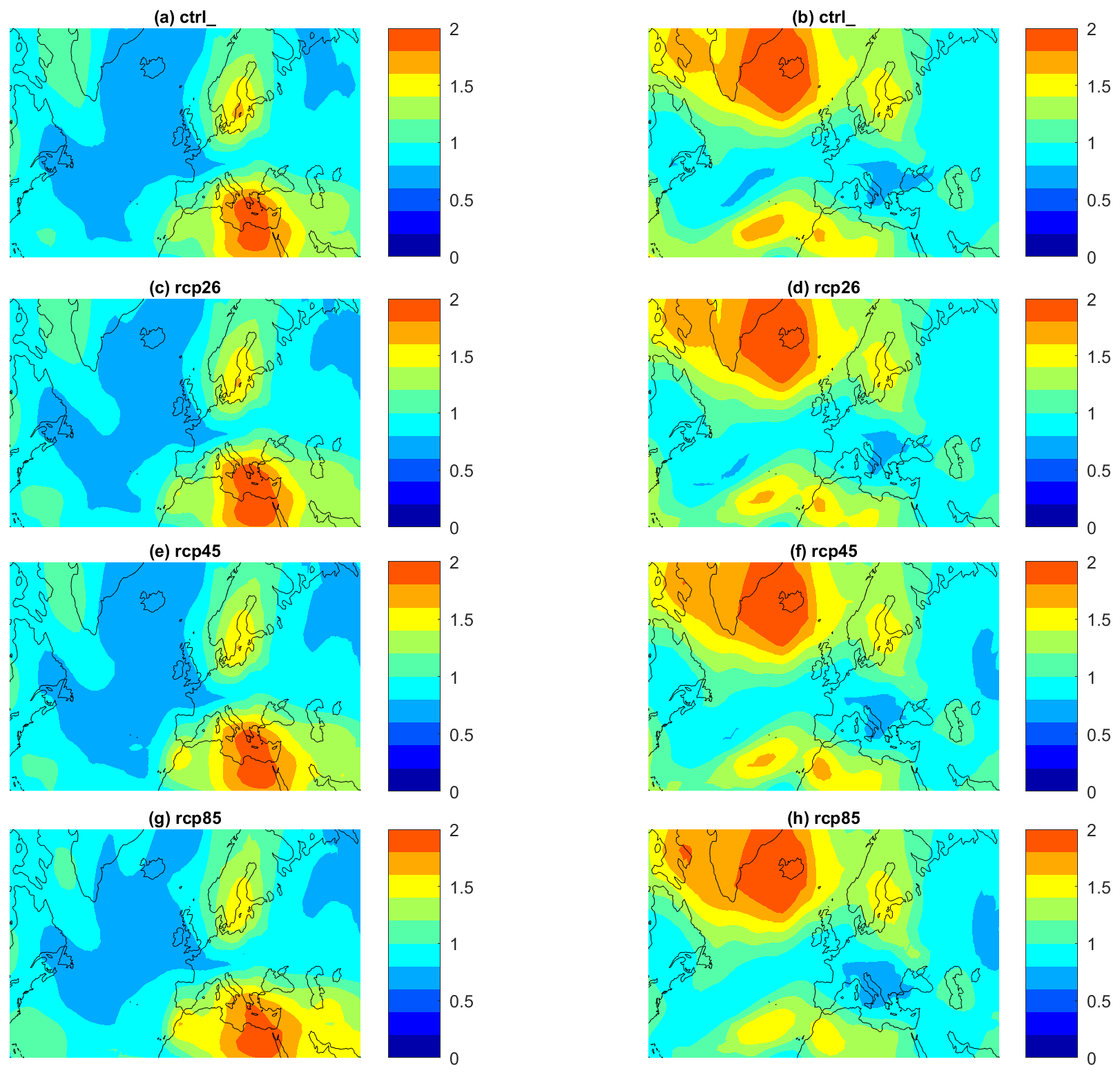
Figure B2 Sea-level pressure uncertainty in PlaSim analogues: root mean squared difference in standardized sea-level pressure (standard deviations) between analogues and cluster centroids for cluster 1 (a, c, e, g) and cluster 2 (b, d, f, h). (a, b) Control run. (c, d) RCP2.6 run. (e, f) RCP4.5 run. (g, h) RCP8.5 run.

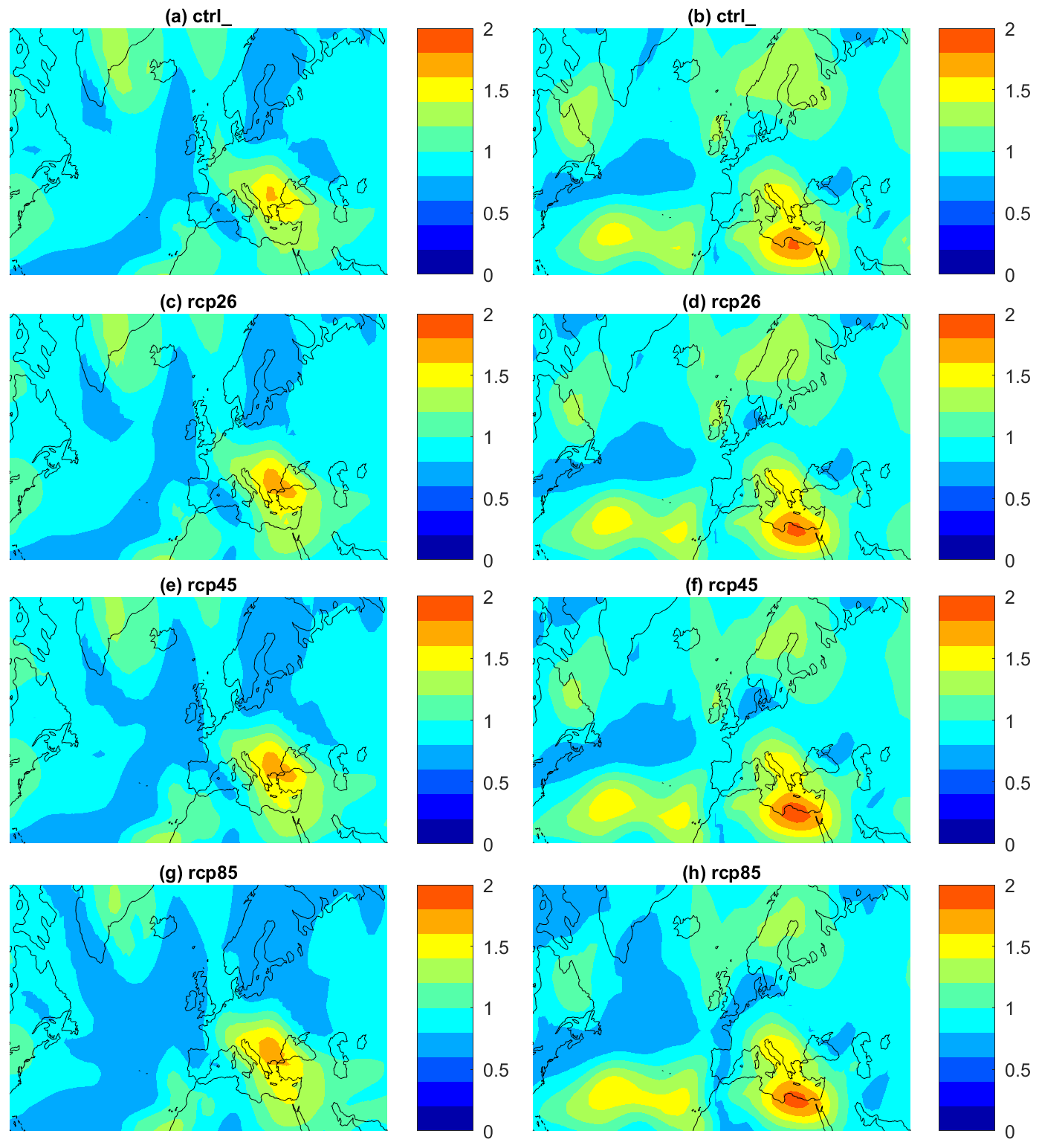
Figure B3 The figure shows 850 hPa temperature uncertainty in PlaSim analogues: root mean squared difference in standardized 850 hPa temperature (standard deviations) between analogues and cluster centroids for cluster 1 (a, c, e, g) and cluster 2 (b, d, f, h). (a, b) Control run. (c, d) RCP2.6 run. (e, f) RCP4.5 run. (g, h) RCP8.5 run.

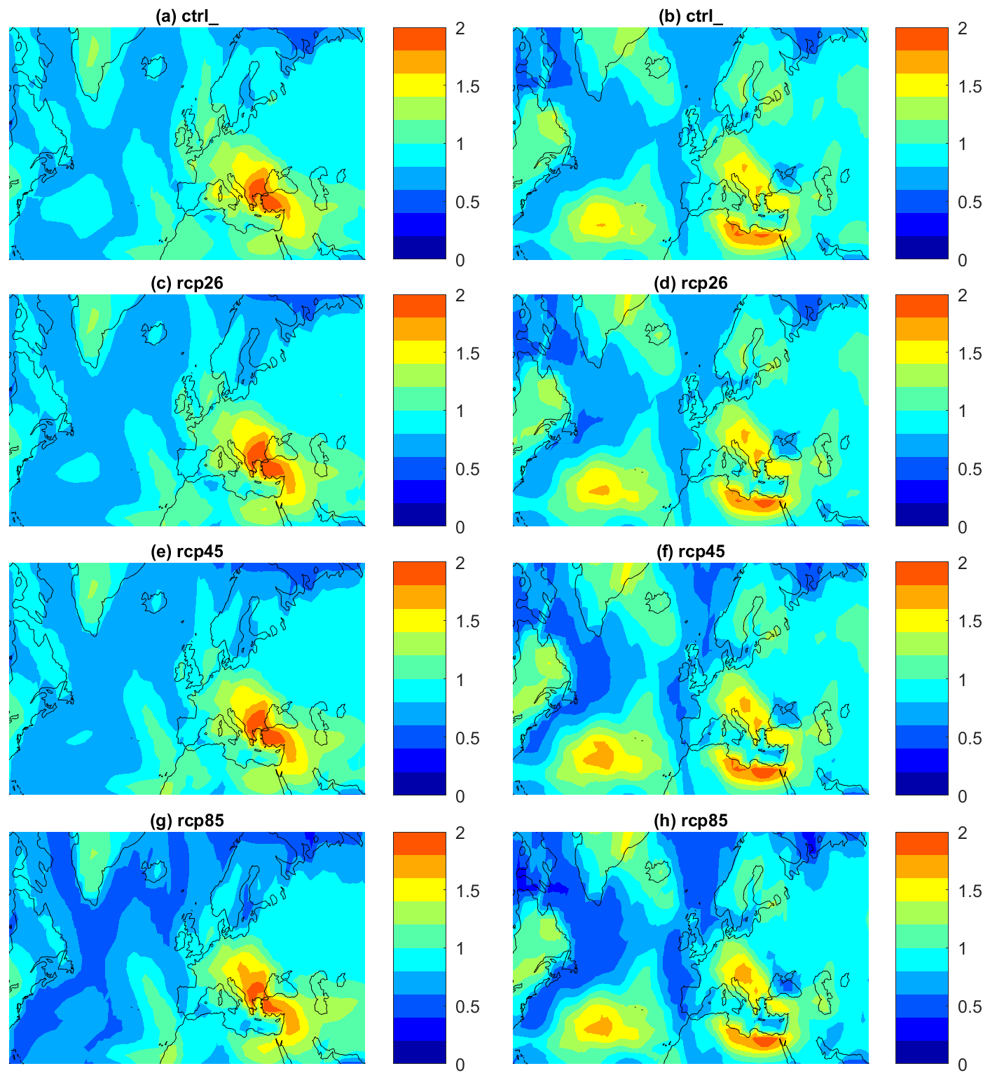
Figure B4 The figure shows 2 m temperature uncertainty in PlaSim analogues: root mean squared difference in standardized 2 m temperature (standard deviations) between analogues and cluster centroids for cluster 1 (a, c, e, g) and cluster 2 (b, d, f, h). (a, b) Control run. (c, d) RCP2.6 run. (e, f) RCP4.5 run. (g, h) RCP8.5 run.

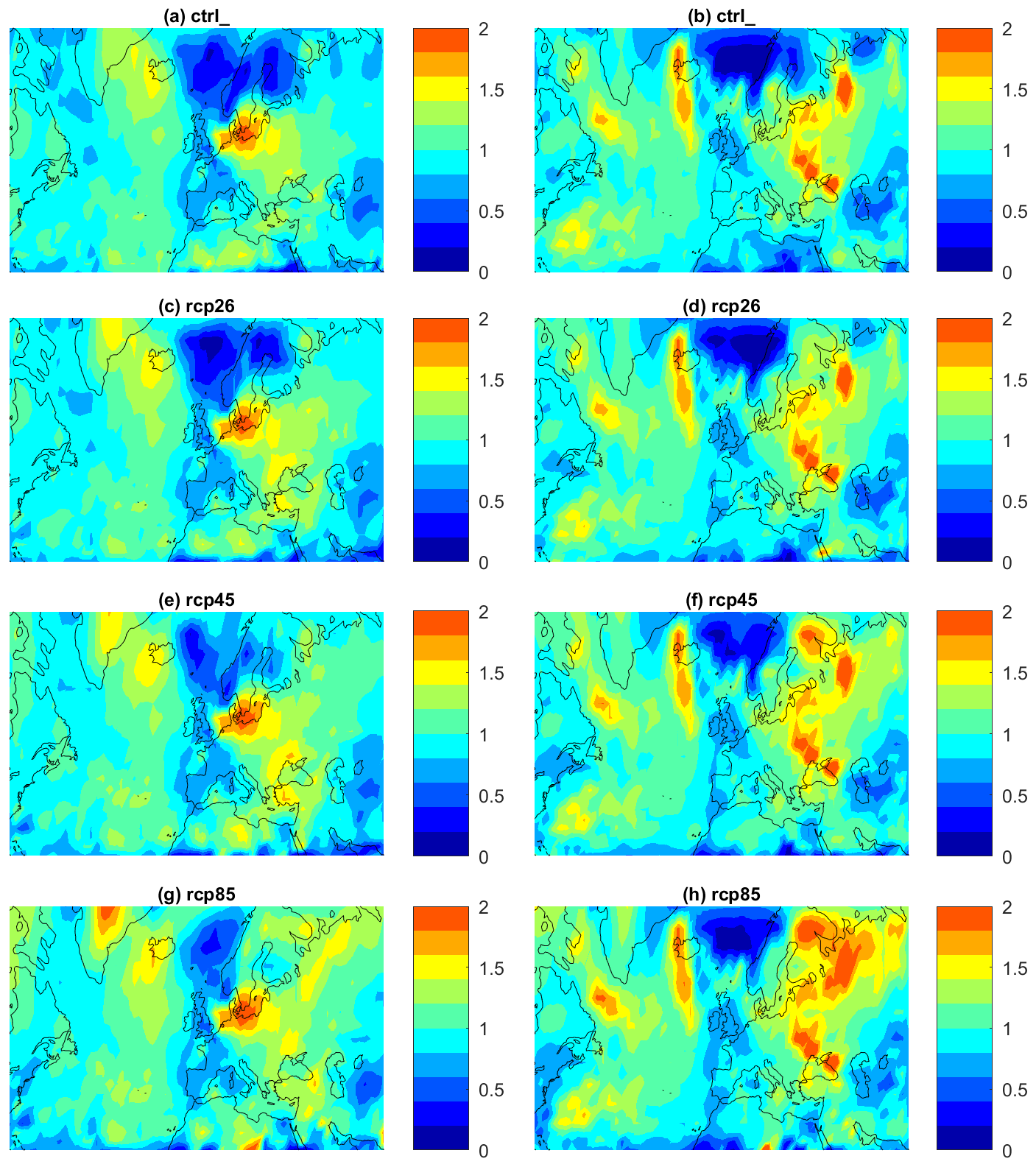
Figure B5 Daily precipitation rate uncertainty in PlaSim analogues: root mean squared difference in standardized daily precipitation rates (standard deviations) between analogues and cluster centroids for cluster 1 (a, c, e, g) and cluster 2 (b, d, f, h). (a, b) Control run. (c, d) RCP2.6 run. (e, f) RCP4.5 run. (g, h) RCP8.5 run.