the Creative Commons Attribution 4.0 License.
the Creative Commons Attribution 4.0 License.
 | 28 Apr 2022
MESMER-M: an Earth system model emulator for spatially resolved monthly temperature
Shruti Nath
Quentin Lejeune
Lea Beusch
Sonia I. Seneviratne
Carl-Friedrich Schleussner
The degree of trust placed in climate model projections is commensurate with how well their uncertainty can be quantified, particularly at timescales relevant to climate policy makers. On inter-annual to decadal timescales, model projection uncertainty due to natural variability dominates at the local level and is imperative to describing near-term and seasonal climate events but difficult to quantify owing to the computational constraints of producing large ensembles. To this extent, emulators are valuable tools for approximating climate model runs, allowing for the exploration of the uncertainty space surrounding selected climate variables at a substantially reduced computational cost. Most emulators, however, operate at annual to seasonal timescales, leaving out monthly information that may be essential to assessing climate impacts. This study extends the framework of an existing spatially resolved, annual-scale Earth system model (ESM) emulator (MESMER, Beusch et al., 2020) by a monthly downscaling module (MESMER-M), thus providing local monthly temperatures from local yearly temperatures. We first linearly represent the mean response of the monthly temperature cycle to yearly temperatures using a simple harmonic model, thus maintaining month-to-month correlations and capturing changes in intra-annual variability. We then construct a month-specific local variability module which generates spatio-temporally correlated residuals with yearly temperature- and month-dependent skewness incorporated within. The emulator's ability to capture the yearly temperature-induced monthly temperature response and its surrounding uncertainty due to natural variability is demonstrated for 38 different ESMs from the sixth phase of the Coupled Model Intercomparison Project (CMIP6). The emulator is furthermore benchmarked using a simple gradient-boosting-regressor-based model trained on biophysical information. We find that while regional-scale, biophysical feedbacks may induce non-uniformities in the yearly to monthly temperature downscaling relationship, statistical emulation of regional effects shows comparable skill to the more physically informed approach. Thus, MESMER-M is able to statistically generate ESM-like, large initial-condition ensembles of spatially explicit monthly temperature fields, providing monthly temperature probability distributions which are of critical value to impact assessments.
- Article
(18051 KB) - Full-text XML
- BibTeX
- EndNote


Climate model emulators are computationally inexpensive devices that derive simplified statistical relationships from existing climate model runs to then approximate model runs that have not been generated yet. By reproducing runs from deterministic, process-based climate models at a substantially reduced computational time, climate model emulators facilitate the exploration of the uncertainty space surrounding model representation of climate responses to specific forcings. A wide toolset of Earth system model (ESM) emulators exists with capabilities ranging from investigating the effects of greenhouse gas (GHG) emission scenarios on global and regional mean annual climate fields (Meinshausen et al., 2011; Tebaldi and Arblaster, 2014) to looking at regional-scale annual, seasonal, and monthly natural climate variabilities (McKinnon and Deser, 2018; Alexeeff et al., 2018; Castruccio et al., 2019; Link et al., 2019).
Recently, the Modular Earth System Model Emulator with spatially Resolved output (MESMER) (Beusch et al., 2020) has been developed with the ability to statistically represent ESM-specific forced local responses alongside projection uncertainty arising from natural climate variability. It does so using a combination of pattern scaling and a natural climate variability module, to generate grid point level, yearly temperature realizations that emulate the properties of ESM initial-condition ensembles. By training on different ESMs individually, MESMER is furthermore able to account for inter-ESM differences in forced local responses and natural climate variability, thus approximating a multi-model initial-condition ensemble, i.e. a “super-ensemble”. The probability distributions of grid point level, yearly temperatures generated by MESMER could be especially relevant when used as input data for simulation of impacts that depend on this variable. MESMER thus offers the perspective of improving our description of the likelihood of future impacts under multiple future climate scenarios.
Considering the importance of monthly and seasonal information when assessing the impacts of climate change (Schlenker and Roberts, 2009; Wramneby et al., 2010; Stéfanon et al., 2012; Zhao et al., 2017), extending the MESMER approach to grid point level monthly temperatures appears desirable. Such an approach holds additional value in assessing the evolving likelihoods of future impacts, as the temperature response at monthly timescales displays non-uniformities that are distributed onto monthly variabilities and therefore uncertainties, which are otherwise unapparent at annual timescales. In particular, winter months can warm disproportionately more than summer months (Fischer et al., 2011; Holmes et al., 2016; Loikith and Neelin, 2019), which in turn leads to non-stationarity in the amplitude of the seasonal cycle (i.e. intra-annual temperature variabilities) with evolving yearly temperatures (i.e. the intra-annual temperature response is heteroscedastic with regard to yearly temperature) (Fischer et al., 2012; Huntingford et al., 2013; Thompson et al., 2015; Osborn et al., 2016). Additionally, given that monthly temperature distributions have been observed to display non-Gaussianity, evolving yearly temperatures may cause disproportionate effects on their tail extremes, leading to changes in skewness (Wang et al., 2017; Sheridan and Lee, 2018; Tamarin-Brodsky et al., 2020).
This study focuses on extending MESMER's framework by a local monthly downscaling module (MESMER-M). This enables the estimation of projection uncertainty due to natural variability as propagated from annual to monthly timescales since MESMER-M builds upon MESMER, which has already been validated as yielding spatio-temporally accurate variabilities. In constructing MESMER-M, we furthermore place emphasis on representing heteroscedasticity of the intra-annual temperature response as well as changes in skewness of individual monthly distributions in a spatio-temporally accurate manner. The structure of this study is as follows: we first introduce the framework of the emulator in Sect. 3.1 and the approach to verification of the emulator performance in Sect. 3.2; we then provide the calibration results of the emulator in Sect. 4 and verification results in Sect. 5, after which we proceed to the conclusion and outlook in Sect. 6.
In the analysis, 38 CMIP6 models (Eyring et al., 2016) are considered, using simulations for the SSP5-8.5 high-emission scenario (O'Neill et al., 2016), so as to first explore the emulator's applicability to the extreme end of GHG-induced warming. Where an ESM's initial-condition ensemble set contains more than one member, it is split into a training set (used for emulator calibration) and a test set (used for emulator cross-validation). Systematic approaches in getting the best train–test split exist, such as that employed by Castruccio et al. (2019), which requires the presence of a large ensemble and compromises between stability in inference (represented for example by variability) of the emulator and the computational time for training it. Since the primary purpose of MESMER-M is to provide the best possible emulations based on available training material, such approaches are optional however and would only limit the demonstration of MESMER-M to CMIP6 ESMs with large ensembles. Here we implement a simple 70 %–30 % (and for models with more than 20 ensemble members a 50 %–50 %) train–test split so as to maintain a good balance between training time and emulator performance. A summary of the CMIP6 models used, their associated modelling groups, and the initial-condition ensemble members present within the training and test sets are given in Table A1. All ESM runs are obtained at a monthly resolution and are bilinearly interpolated to a spatial resolution of (Brunner et al., 2020). The emulator is trained using yearly averaged temperature as predictor values. The term “temperature” here refers to anomalies of surface air temperature (standard name, “tas”) relative to the annual climatological mean over the reference period of 1870–1899.
3.1 MESMER
MESMER is an ESM-specific emulator built to statistically produce spatially resolved, yearly temperature fields by considering both the local mean response and the local variability surrounding the mean response. Within MESMER, local temperatures T for a given grid point s and year y are emulated as follows (Beusch et al., 2020):
where gs is the local mean response to global mean temperatures Tglob and consists of a multiple, linear regression on the forced Tglob,forced (capturing the smooth trend in Tglob) and variability Tglob,var components of Tglob, with coefficients and respectively and intercept term . More details on the extraction and representation of Tglob,forced and Tglob,var can be found in Beusch et al. (2020). ηs,y represents the residual variability around the mean response.
3.2 MESMER-M
We divide MESMER-M into a mean response module and a residual variability module, each calibrated on ESM simulation output data at each grid point individually according to the procedure described in this section and summarized in Fig. 1. Such division of a modelling exercise has been applied to other climate model emulators (Tebaldi and Arblaster, 2014; Alexeeff et al., 2018; Link et al., 2019; Beusch et al., 2020) and comes with its underlying assumptions. The primary assumption in our case is that the ESM monthly temperatures are distinctly separable into a mean response component and a residual variability component. Traditionally the mean response module is designed to be dependent on a certain forcing (in this case local, yearly temperatures), while the variability module is space–time-dependent (i.e. varying with time and across the spatial domain). Given the expected changes in monthly skewness with evolving yearly temperature however, we furthermore propose both a space–time- and yearly-temperature-dependent variability module. Other forcings, such as land cover changes, are furthermore assumed to have considerably smaller impacts on the monthly temperature response and are thus not explicitly included. Given the modular approach taken, this assumption could be addressed in the future with the addition of separate modules which isolate the signals of such other forcings.
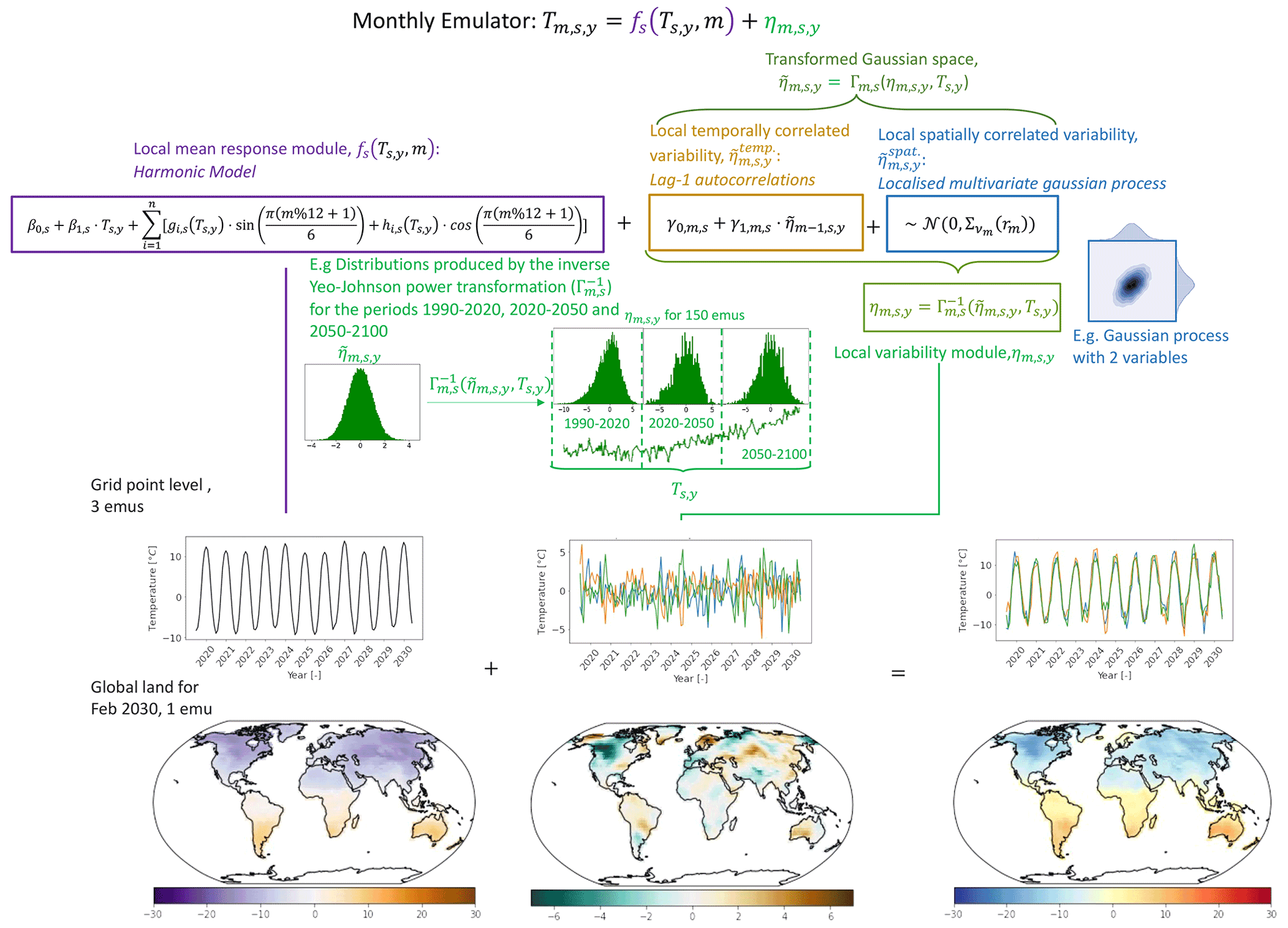
Figure 1Modular framework for the monthly emulator illustrated for an example ESM. The local mean response module is represented using a harmonic model (Fourier series). The local variability module starts with a Yeo–Johnson transformation before fitting the AR(1) process (distinguished into temporally varying and spatially varying components). An inverse Yeo–Johnson transformation is applied to emulated realizations drawn from the AR(1) process. A schematic illustrating the inverse Yeo–Johnson transformation's representation of the residual distribution skewness (grouped into the periods 1990–2020, 2020–2050, and 2050–2100) with evolving yearly temperatures (plotted below the distributions) is provided. Example data for the multivariate Gaussian process used within are also given. Three emulation examples (“emu” in the figure) are shown as time series for one grid point, and one emulation example is also shown as a global map.
3.2.1 Mean response module
The mean response module was conceived to represent the grid point level mean response of both monthly temperature values and the amplitudes of the seasonal cycle (intra-annual variability) to changing yearly temperatures. We employ a harmonic model consisting of a Fourier series with amplitude terms fitted as linear combinations of yearly temperature, centred around a linear function of yearly temperature as shown in Eq. (2):
where T is temperature, m, s, and y refer to month, space (i.e. grid point), and year indexes, % is modulo, and gi and hi are linear functions of T for the ith ordered term of the Fourier series. Since the monthly cycle revolves around its yearly temperature, fitting results for β0 and β1 coefficients had negligible effects (β0=0 and β1=1), and for simplicity's sake, we show the Fourier series as centred around yearly temperature values within the following sections. In choosing the order (n) of the harmonic model, we optimized between model complexity and accuracy using the Bayesian information criterion (BIC). For this, harmonic models with orders n=1, …, 6 were fitted at each grid point and their BIC scores calculated, from which the order with the lowest score was chosen. It should be acknowledged that this approach may lead to a higher number of terms selected as temporal independence in model performance is assumed.
3.2.2 Residual variability module
The local residual variability (otherwise simply called “residuals”), i.e. the difference between actual local monthly temperature and its mean monthly response to variations in local yearly temperature (given by the harmonic model), is assumed to be solely a manifestation of intra-annual variability processes. It can thus be thought of as short-term spatio-temporally correlated patterns. Similar to previous MESMER developments, we represent the residual variability using an AR(1) process. Since the residual variability distributions display month-dependent skewness (see example Shapiro–Wilk test for January and July in Appendix B), which is non-stationary with regard to yearly temperatures, we first transform them into a stationary Gaussian space before fitting the AR(1) process. This strategy has already been pursued in problems concerning skewness in residual precipitation variability (Frei and Isotta, 2019). Precisely, we use the monotonic Yeo–Johnson transformation (Γm,s), which accounts for both positive and negative data values, to locally normalize monthly residuals (Yeo and Johnson, 2000).
Γm,s relies on a λ parameter to deduce the shape of a distribution and normalize accordingly. Non-stationarity in month-specific residual skewness with regard to yearly temperature is taken into account by defining the λ parameter as a logistic function of yearly temperature, as shown in Eq. (4):
where and are coefficients fitted using maximum likelihood. The performance improvement of having a parameter that is dependent on yearly temperature compared to a case where it is invariant (λm,s) is demonstrated by additional tests shown in Appendix C (shown for January and July). Since the majority of ESMs profit from yearly temperature dependence in λ, we use in all ESMs.
The AR(1) process is applied to the residual variability terms after they are locally normalized as according to Eq. (3). Following the approach of Beusch et al. (2020), temporal correlations are accounted for in the deterministic component of the AR(1) process, whereas spatial correlations are accounted for in its noise component, and hence can be expressed as shown in Eq. (5):
where is the locally normalized residual variability at month, grid point, and year m, s, and y and and are its respective temporally varying and spatially varying components.
The AR(1) process accounts for autocorrelations up to a time lag of 1 and is suited in representing the residual variability, which is assumed to have rapidly decaying covariation such that longer-term patterns (if any) covary with yearly temperature. is shown in Eq. (6):
where and are coefficients fitted per month. is constrained between −1 and 1.
Following this, (i.e. the noise component of the AR(1) process) needs to account for the spatial cross-correlations between grid points. It is modelled through a localized monthly multivariate Gaussian process and thus dampens spatial covariations with increasing distance, as shown in Eq. (7):
where is a multivariate Gaussian process with a mean of 0 and covariance matrix . As the number of land grid points is much higher than the number of temperature field samples, is rank deficient and is thus localized by point-wise multiplication with the smooth Gaspari–Cohn correlation function (Gaspari and Cohn, 1999), which has exponentially vanishing correlations with distance rm and was used in previous MESMER fittings (Beusch et al., 2020). rm is chosen per month in a similar cross-validation with a leave-one-out approach as previous MESMER fittings (Beusch et al., 2020) using distances of 1500 to 8000 km at 250 km intervals. The localized empirical covariance matrix, , is derived analytically based on the mathematical expectations for the covariance of noise terms of an AR(1) process (Matalas, 1967; Richardson, 1981), as shown in Eq. (8):
where is the empirical covariance matrix constructed across all grid points for a given month from the locally normalized empirical residuals. When generating emulated realizations from the AR(1) process, we apply the inverse Yeo–Johnson transformation to obtain the final residual variability terms.
3.3 Evaluating emulator performance
3.3.1 Mean response verification
To evaluate how well the monthly cycle's mean response, , is captured, we calculate Pearson correlation coefficients between the emulated values obtained from the harmonic model and their training run values across the whole globe for each month, with each grid point weighted equally. This not only gives an idea of how well the magnitudes of mean response changes correspond but also how in phase the emulated monthly cycles are with training run monthly cycles. Where test runs are available, their correlations to the harmonic-model results are also calculated to assess how well the harmonic model can represent data it has not been trained on. Ideally, the test run correlations should be equal to those of the training runs, with anything substantially lower indicating overfitting and anything substantially higher indicating a non-representative training set (i.e. further modifications in the train-to-test splitting would have to be considered).
3.3.2 Residual variability verification
In order to evaluate how well the emulator reproduces the deviations from the harmonic model simulated by the ESMs, 50 emulations are generated per training run. First, we check that short-term temporal features are sufficiently captured for each individual grid point. To distinguish such short-term temporal features, we isolate the high-frequency temporal patterns present within the residual variability: each residual variability sequence is decomposed into its continuous power spectra, from which we verify, by computing Pearson correlation coefficients, that the top 50 highest-frequency bands within the training run residual variabilities appear with similar power spectra in the corresponding emulated residual variabilities. Second, we verify how well the spatial covariance structure is preserved by calculating monthly spatial cross-correlations across the residuals produced by each individual emulation and, by using Pearson correlations, comparing them to those of their respective training runs. Where test runs are available, a similar verification between them and training runs is done, thus yielding an approximation of how actual ESM initial-condition ensemble members would relate to each other.
3.3.3 Regional-scale ensemble reliability verification
The full emulator, consisting of both the mean response (i.e. harmonic model) and residual variability modules, is evaluated for its representation of regional, area-weighted average monthly temperatures of all 26 SREX regions (Seneviratne et al., 2012; see Appendix D for details on SREX regions) at each individual month. Global land results always constitute area-weighted averages across all land grid points excluding Antarctica. We assess how well the emulator can reproduce the 5th, 50th, and 95th quantiles of the respective ESM initial-condition ensemble over the periods of 1870–2000 and 2000–2100, by means of quantile deviations as previously done by Beusch et al. (2020). A step-by-step process for calculating monthly quantile deviations of the ESM from the emulator is as follows.
-
Calculate the area-weighted regional average of a given SREX region for each ESM run and each of its respective emulations at a given month.
-
Extract the qth emulated quantile at each time step from the set of regionally averaged emulations.
-
Within a defined time period (e.g. 1870–2000), calculate the proportion of time steps for which the regionally averaged ESM value is less than the respective emulated qth quantile value. The resulting number is qESM.
-
The quantile deviation of the ESM from the emulator is then given as qESM−q.
By drawing comparisons between the quantile deviations obtained in the two time periods considered, we can evaluate whether inter-annual variations in monthly temperature distributions are sufficiently captured. Since the magnitude of global warming varies between both time periods, such a comparison will additionally help identify whether the emulator sufficiently captures the expected changes in temperature skewness under changing climatic conditions (Wang et al., 2017; Sheridan and Lee, 2018; Tamarin-Brodsky et al., 2020).
3.4 Benchmarking MESMER-M using a simple physically informed approach
Any variability in monthly temperatures that cannot be explained by variability in yearly temperature alone is stochastically accounted for in MESMER-M's local residual variability module (see Sect. 3.2.2), following existing downscaling theory (Berner et al., 2017; Arnold, 2001). Hence, month- and season-dependent variability linked to physical drivers such as atmosphere–ocean interactions (Neale et al., 2008; Deser et al., 2012), e.g. the El Niño–Southern Oscillation (ENSO), and biophysical feedbacks (Potopová et al., 2016; Xu and Dirmeyer, 2011; Jaeger and Seneviratne, 2011; King, 2019; Tamarin-Brodsky et al., 2020), e.g. snow–albedo feedbacks, is not explicitly modelled but instead represented by a stochastic process. Nevertheless, first-order changes in the characteristics of these variabilities across warming levels can be approximated within MESMER-M since the skewness of MESMER-M's residual variability emulations depends on the yearly temperature. In this section, we delineate a framework to verify that this statistical approach, based on a single input variable of yearly temperature, can sufficiently imitate properties of the monthly temperature response which otherwise result from intra-annual variability processes. We primarily verify for representation of secondary biophysical feedbacks as biophysical variables are obtainable as direct output from the ESMs, whereas accounting for modes of climate variability and atmospheric processes would require further data processing and analysis. Furthermore, some effects of atmospheric processes can follow from or manifest themselves in biophysical variables, e.g. as seen by Allen and Zender (2011), and hence are indirectly accounted for by using biophysical variables.
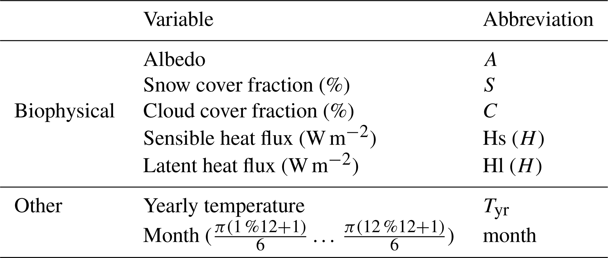
To isolate the contribution of secondary biophysical feedbacks to the monthly temperature response, we consider them as inducing the residual differences between the ESM and harmonic-model realizations. This follows from the harmonic model representing the expected direct mean response to evolving yearly temperatures, with any systematic departure from it being driven by secondary forcers. To rudimentarily represent these contributions, a simple, physically informed model consisting of a suite of gradient-boosting regressors (GBRs) (Hastie et al., 2009) is built for each ESM. Each GBR within the suite is calibrated over one grid point and is trained to predict the local residual differences using local biophysical variable values (see Table 1) as predictors. Predictors are chosen so as to best represent the intra-annual variation in radiative and thermal fluxes alongside their evolution under changing yearly temperatures. The list of predictors is complemented by local yearly temperature values and month values in their harmonic form (hence , n=1 for January, etc.) to account for month dependencies in the residual differences and yearly temperature influences (if any) left behind within the residuals.
To optimize the selection of the biophysical variables used as predictors, we first compare the performance of different physically informed models trained using different sets of biophysical variables for each ESM. The best globally performing model is selected as a benchmark to assess how well the residual variability module, described in Sect. 3.2.2, statistically represents properties within the monthly response arising from secondary biophysical feedbacks. Pearson correlations, between ESM test runs and harmonic-model test results augmented by biophysical variable, Tyr and month-based physically informed model predictions are calculated. As a measure of performance, the aforementioned correlation values are given relative to those obtained when augmenting using only Tyr and month-based physically informed model predictions. This additionally allows the determination of whether improvement in residual representation comes from the added biophysical variable information. As we are most interested in the representation of monthly temperature distributions and the influences of biophysical feedbacks therein, we consider the energy distances of the benchmark, “physically informed” emulations – constituting the mean response with GBR-predicted residuals added on top – from the actual ESM runs and compare them to the energy distances of the statistical emulations – constituting the mean response with residuals from the residual variability module added on top (as described in Sect. 3.2) – from the actual ESM runs. The energy distance is a non-parametric estimate of the distance between two cumulative distribution functions (cdfs), x and y, by considering all their independent pairs of variables, Xi, Xj (i.e. pairs of physically informed/statistical emulated values) and Yk, Yl (i.e. pairs of actual ESM values) respectively.
Time series of the biophysical variables are obtained from CMIP6 runs. For this analysis, we only focus on ESMs which provided data for all five biophysical variables under consideration, for both the test and training runs used during emulator calibration.
Table 1List of biophysical variables used in training the gradient boosting regressor.
4.1 Calibration results
When calibrating the harmonic model constituting the mean response module, the highest orders of the Fourier series were found in tropical to sub-tropical regions where the seasonal cycle has a relatively low amplitude (first row, Fig. 2). The Arctic also displays relatively high orders chosen within the Fourier series, possibly due to higher variabilities in the response of the seasonal cycle shape with increasing yearly temperatures. In contrast, temperate regions which possess distinctly sinusoidal seasonal cycles with marked snow-driven summer to winter transitions display relatively lower orders. CanESM5 and MIROC6 show the overall highest orders, which can be tracked back to them having more training runs, and hence more information on which to train the emulator, allowing for more model complexity without compromising on accuracy (refer to Table A1).
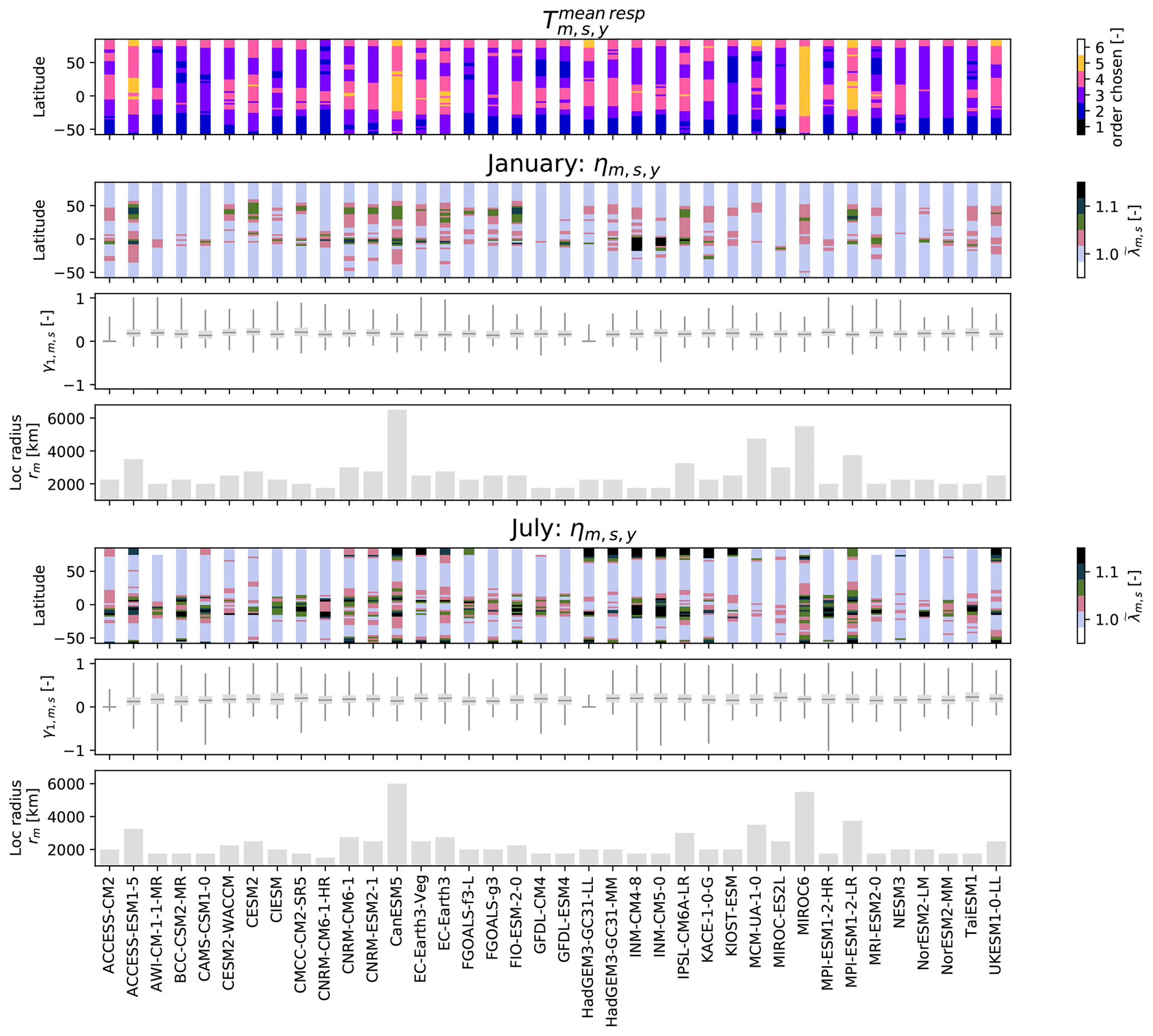
Figure 2Calibration parameters obtained from emulator fittings for all CMIP6 models. For the mean response module, the latitudinally averaged order of the Fourier series considered in the harmonic model is plotted against latitude (row 1). For the monthly residual variability module, parameters are displayed for January (rows 2–4) and July (rows 5–7). coefficients averaged over latitude and all years for the local Yeo–Johnson transformation are plotted against latitude (rows 2 and 4). The local lag-1 autocorrelation coefficients () are plotted as boxplots (rows 3 and 6) with whiskers covering the 0 to 1 quantile range, and the localization radii (rm) are given as bar charts (rows 4 and 7).
The residual variability module calibration results are shown in Fig. 2 for January and July. The average Yeo–Johnson parameter () displays a shift of values greater than 1 to values close to 1 in the Northern Hemisphere (30–50∘) between January and July. In general, values greater (less) than 1 indicate a concave (convex) transformation function owing to negative (positive) skewness, while values equal to 1 suggest minimal skewness in the input distribution (Yeo and Johnson, 2000). This explains the seasonality in as we expect a more negatively skewed residual distribution in the northern hemispheric winter when the snow–albedo feedback leads to a non-linear wintertime warming (Cohen and Rind, 1991; Hall, 2004; Colman, 2013; Thackeray et al., 2019) causing the harmonic model to overestimate the mean temperature response. July displays significantly high values for polar latitudes (>80∘) explainable by the sudden increase in warming rates during ice-free summers (Blackport and Kushner, 2016). Around the Equator (−5 to 5∘) we see values consistently higher than 1 especially in the month of July, with INM-CM5-8 and INM-CM5-0 displaying significantly high values. The source of high equatorial values varies model to model but mainly originates from the north-west South America and Sahel regions, alluding to the presence of some non-linear warming response in these regions.
The lag-1 autocorrelation coefficients () mostly exhibit positive values across all ESMs for January, with at least 70 % of grid points having values between 0 and 0.3, suggesting minimal month-to-month memory additional to the seasonal cycle. July shows similar behaviour for across most ESMs, albeit with a larger spread in values. ACCESS-CM2 and HadGEM3-GC31-LL present themselves as outliers here with the bulk of their coefficients centred around 0 for both January and July, indicating negligible autocorrelations.
Localization radii vary from model to model and are generally higher in January than July reflecting seasonal differences in residual behaviour possibly due to northern hemispheric winter snow cover yielding larger spatial patterns. CanESM5 and MIROC6 display notably higher localization radii, which can again be tracked back to them having more training runs: more time steps are available during the leave-one-out cross-validation, thus making it generally possible to robustly estimate spatial correlations up to higher distances, which in turn leads to selecting larger localization radii. It should however be stressed that the ESM itself is the main driver behind the calibration results (e.g. even with only one ensemble member, MCM-UA-1-0 has a high localization radius).
4.2 Regional behaviour for four selected ESMs
To illustrate the regional behaviour of the calibrated emulator, we focus on four select ESMs. Figure 3 visually demonstrates the harmonic model constituting the mean response module capturing the mean monthly temperature response for both January and July, at global and regional scales (here we show the SREX regions western North America, WNA, and West Africa, WAF), across all four ESMs. The remaining natural variability surrounding the mean response displays a month dependency across the four ESMs, such that January variabilities are up to double that of July both globally and in the displayed regions. These month dependencies in variabilities are well accounted for within the full emulations comprising both the mean response and the residual variability module, highlighting the necessity of a month-specific residual variability module.
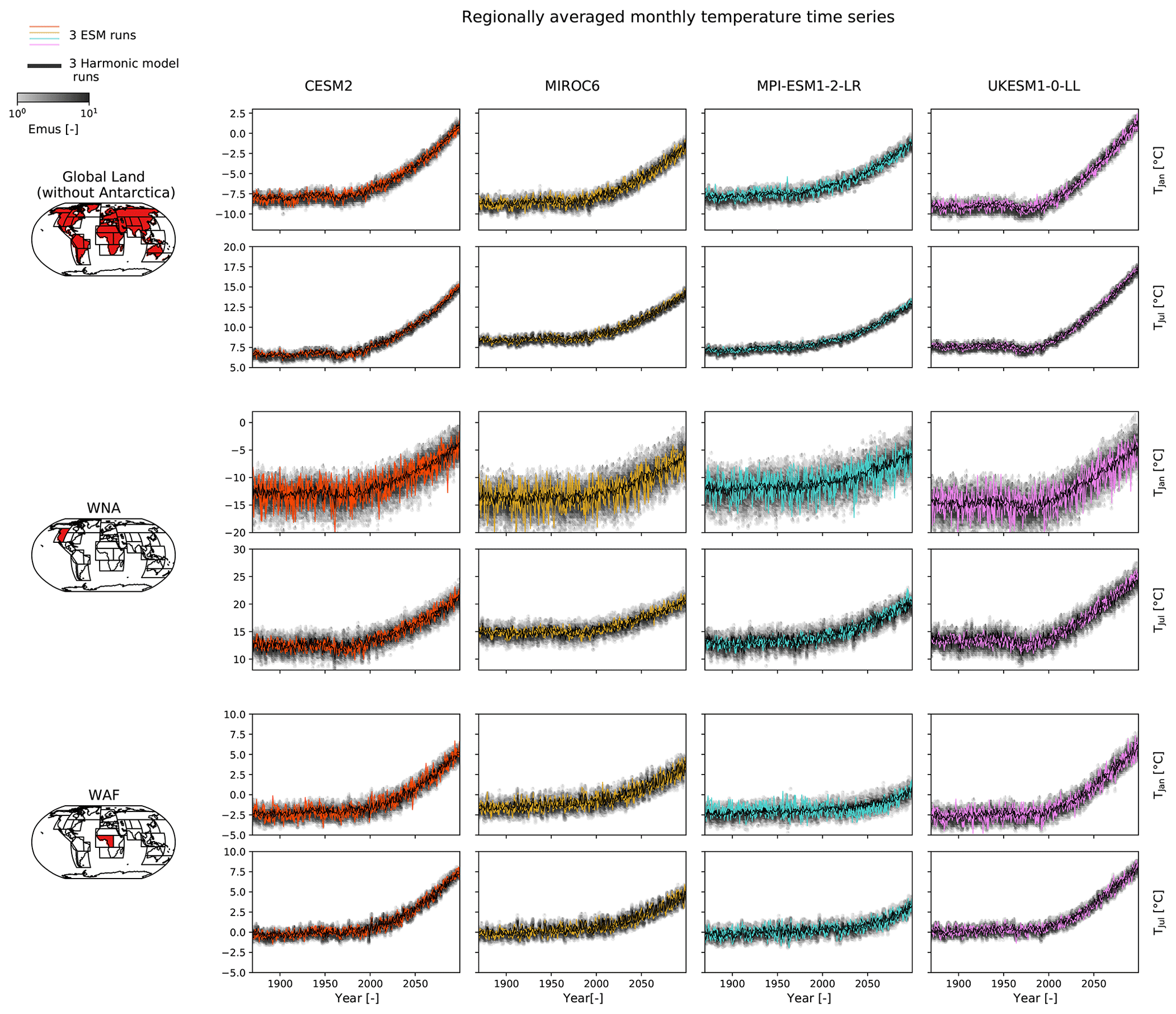
Figure 3Regionally averaged temperature time series (rows) of January and July for four example ESMs (columns). Three ESM ensemble runs (coloured), their respective harmonic-model results (black), and 50 full emulations (emus) for each of the three patterns (grey colour scale) are plotted. Temperature values are given as anomalies with respect to the annual climatological mean over the reference period of 1870–1899. The regions are, from top to bottom, global land without Antarctica, western North America (WNA), and West Africa (WAF).
Figure 4 shows the trends in the variance of each year's monthly temperatures around the yearly mean (i.e. variance in intra-annual temperatures).The harmonic model is able to capture the general trends displayed by the ESMs, albeit not being able to fully account for non-linearities within them. For example, MPI-ESM1-2-LR displays a marked non-linear increase in intra-annual variance with increasing yearly temperatures for WAF, which is misrepresented by the harmonic model as a linear increase. Construction of the physically informed model outlined in Sect. 3.4 elucidated albedo as the main covariant to monthly temperature variability in WAF for MPI-ESM1-2-LR (see Sect. 5.4), indicating changes in land surface properties (possibly due to the reduction in tree cover in this region) as driving intra-annual variance changes. This demonstrates the limitation of solely relying on yearly temperatures as input towards predicting monthly temperatures when other forcings (in this case changes in land surfaces) dominate. Other forcings rarely dominate over the response to yearly temperatures however, and the full emulations are able to capture the overall spread.

Figure 4Regionally averaged variance of intra-annual temperatures (i.e. variance of each year’s monthly temperatures around the yearly mean) scatterplotted against yearly temperature (rows) for four example ESMs (columns).Three ESM ensemble runs (coloured), their respective harmonic-model results (black), and 50 full emulations for each of the three patterns (grey colour scale) are plotted. Temperature values are taken as anomalies with respect to the annual climatological mean over the reference period of 1870–1899. Each dot represents the temperature variance calculated from the monthly values for 1 individual year. The regions are from top to bottom: global land without Antarctica, western North America (WNA), and West Africa (WAF).
5.1 Mean response verification
We evaluate the ability of the harmonic model, constituting the mean response module, in capturing the monthly cycle's response to evolving yearly temperatures. Pearson correlations between the harmonic model and ESM training runs range from 0.7 up to almost 1 (Fig. 5). Summer months (e.g. June) exhibit the highest correlations while transition months of spring (March, April) and autumn (October, November) have the lowest correlations. Such low correlations could result from the inter-annual spread in the timing of snow cover increase and decrease, such that the mean response extracted does not always match individual years. Winter month (e.g. January) correlations are generally higher than those of transition months but lower than those of summer months. This is possibly due to snow–albedo feedbacks, which induce non-linearities into the winter period mean response (Cohen and Rind, 1991; Hall, 2004; Colman, 2013; Thackeray et al., 2019) leading to lower correlations than those of summer months where the response is more linear. Overall the training run correlations correspond well to test run correlations (where available) confirming good data representation within the training set and minimal (if any) model overfitting.
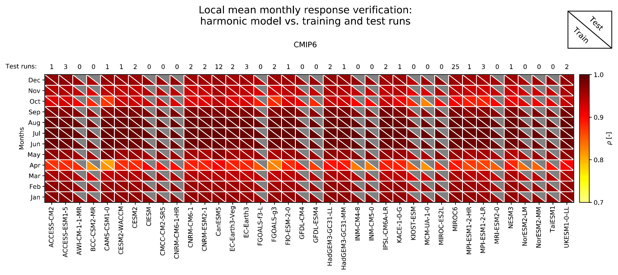
Figure 5Local mean monthly response verification for all CMIP6 models by means of Pearson correlation between the harmonic model and training runs (indicated by the colour of the lower triangle), over all global land grid points (without Antarctica) for each month. The correlations between the harmonic model and test runs are given in colour in the upper triangles to demonstrate how well the harmonic model performs for data it has not seen yet (a grey upper triangle means that no test run is available for this model).
5.2 Residual variability verification
To establish if temporal patterns within the ESM residual variabilities are successfully emulated, the correspondence of their respective power spectra at a grid point level is considered. Results shown in Fig. 6 display the emulator's median correlations with the ESMs' training run power spectra lying between 0.9 and 1. This corresponds well to the correlations across the ESM test runs (crosses). Correlations between the ESM training runs and emulations for a given ESM display very little spread, which is in agreement with the near-identical correlations seen amongst ESM test runs. In the example 2D histogram plot (given for CESM2), we see that the emulator is most successful in capturing lower power-spectra-to-frequency ratios. This may be a consequence of the emulator design, as we restrict ourselves to considering only lag-1 autocorrelations such that lower frequencies with higher power spectra are not accounted for.
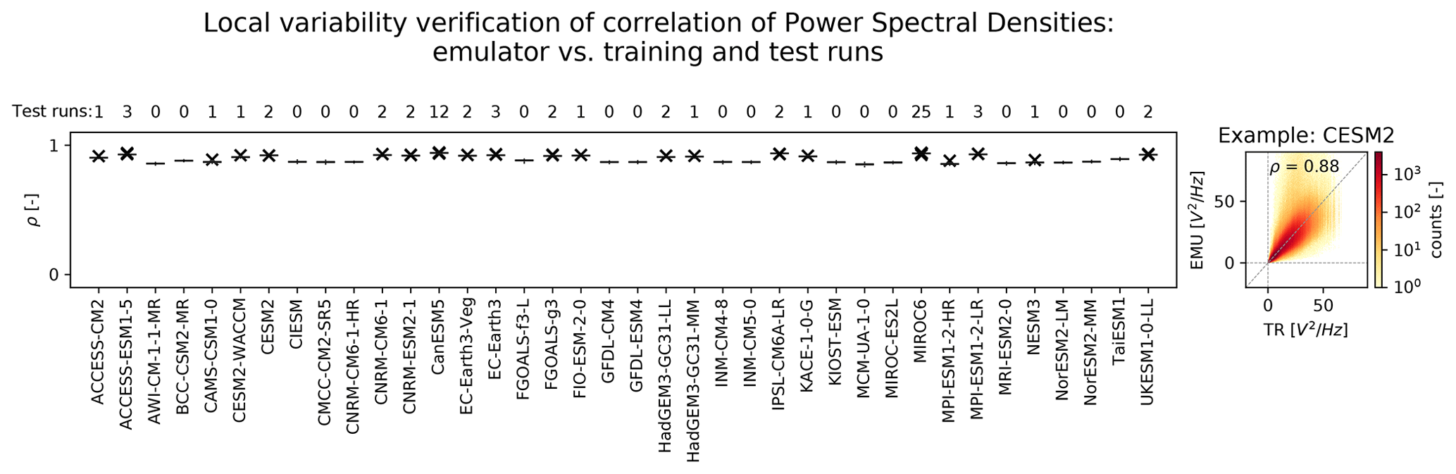
Figure 6Verification of the time component of the local variability module by means of Pearson correlations between the power spectra of the 50 highest-frequency bands present within the training runs (i.e. considering all months together) and the power spectra at which the same 50 frequency bands appear within the respective emulations (boxplots, whiskers indicating 0.05 and 0.95 quantiles) calculated per grid point. Fifty emulations are evaluated per training run. Where test runs are available, their correlations with training runs are also given (black crosses). The example 2D histogram shows the power-spectra-to-frequency ratio for CESM2 training runs versus the corresponding power-spectra-to-frequency ratio within its emulations.
For verification of the residual variability's spatial component, we consider the spatial cross-correlations within four geographical bands centred around the grid point for which temperature is being emulated (Fig. 7) for the example months January and July. As the spatial covariance matrix within the emulator is localized (see Sect. 3.2.2), its spatial cross-correlations are by design expected to diminish with increasing distances. Hence, we see the emulator performing best at distances below 1500 km, with median correlations of 0.91–0.99, which are in line with correlations between ESM test and training runs (crosses). Beyond 1500 km, the emulator performs progressively worse with correlations dropping below 0.1 for distances between 3000 and 6000 km and staying there for distances larger than 6000 km, while those of test runs – where spatial cross-correlations are not localized – remain around 0.5–0.8. CanESM5 and MIROC6 are the two exceptions at distances between 3000 and 6000 km, with correlations of 0.33–0.5, which then again drop to below 0.1 at distances larger than 6000 km. This is due to their notably larger localization radii (see Fig. 2), which leads to a slower decline of spatial cross-correlations with increasing distances as compared to other ESMs.
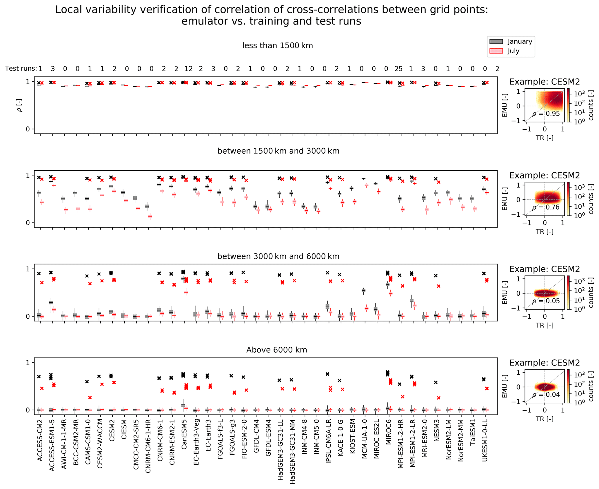
Figure 7Verification of the spatial representation within the local variability module. Pearson correlations between ESM training run and emulated spatial cross-correlations are considered for four geographical bands centred around the grid point for which temperature is being emulated (rows) at individual months of January (black boxplots) and July (red boxplots). Boxplot whiskers indicate 5th and 95th quantiles. Fifty emulations are evaluated per training run. Where ESM test runs are available, their correlations with training runs are also given for January (black crosses) and July (red crosses). Example 2D histograms of the January spatial cross-correlations for CESM2 training runs versus those of its emulations are given for each geographical band.
5.3 Regional-scale ensemble reliability verification
Regionally aggregated 5 %, 50 %, and 95 % quantile deviations of the ESM training (and where available test) runs from the emulated quantiles (derived from the full emulator consisting of both the mean response and local variability module) are plotted over the periods of 1870–2000 and 2000–2100 for the example months January (Figs. 8 and 10) and July (Figs. 9 and 11). The 50 % quantile deviations over the period of 1870–2000 in January and July (Figs. 8 and 9 respectively) generally show low magnitudes (−3 % to 3 %). A slight regional dependency for this period is visible, where tropical/sub-tropical regions of AMZ, NEB, SSA, WAF, EAF, and SAF have generally warmer (colder) emulated 50 % quantiles as compared to the ESM runs, while those of the remaining regions are colder (warmer) for January (July). While January 50 % quantile deviations over the period of 2000–2100 remain low with less (if any) distinguishable regional dependency, July 50 % quantile deviations for this period increase (−10 % to 10 %) with an opposite pattern in regional dependency to that of 1870–2000. The increase for July in deviations could be a combined result of non-linear warming and relatively lower variability in July temperature values as compared to those of January in the ESM simulations. This would indicate a limitation in the emulator's design, where delegating the representation of non-uniformities in the monthly temperature response to the residual variability module does not fully work in the presence of lower variabilities.
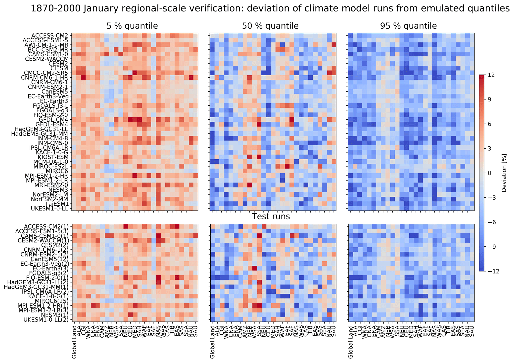
Figure 8January 5 % (left), 50 % (middle), and 95 % (right) quantile deviations (colour) of the climate model runs from the emulated quantiles of the ESM training (top block) and test (bottom block) run values from their monthly emulated quantiles, over the period 1870–2000 for global land (without Antarctica) and SREX regions (columns) across all CMIP6 models (rows). The monthly emulated quantile is computed based on 50 emulations per ESM run, and quantile deviations are given as averages across the respective number of ESM training/test runs. The number of test runs averaged across is indicated in brackets next to the model names in the bottom block. Red means that the emulated quantile is warmer than the quantile of the ESM run and vice versa for blue.
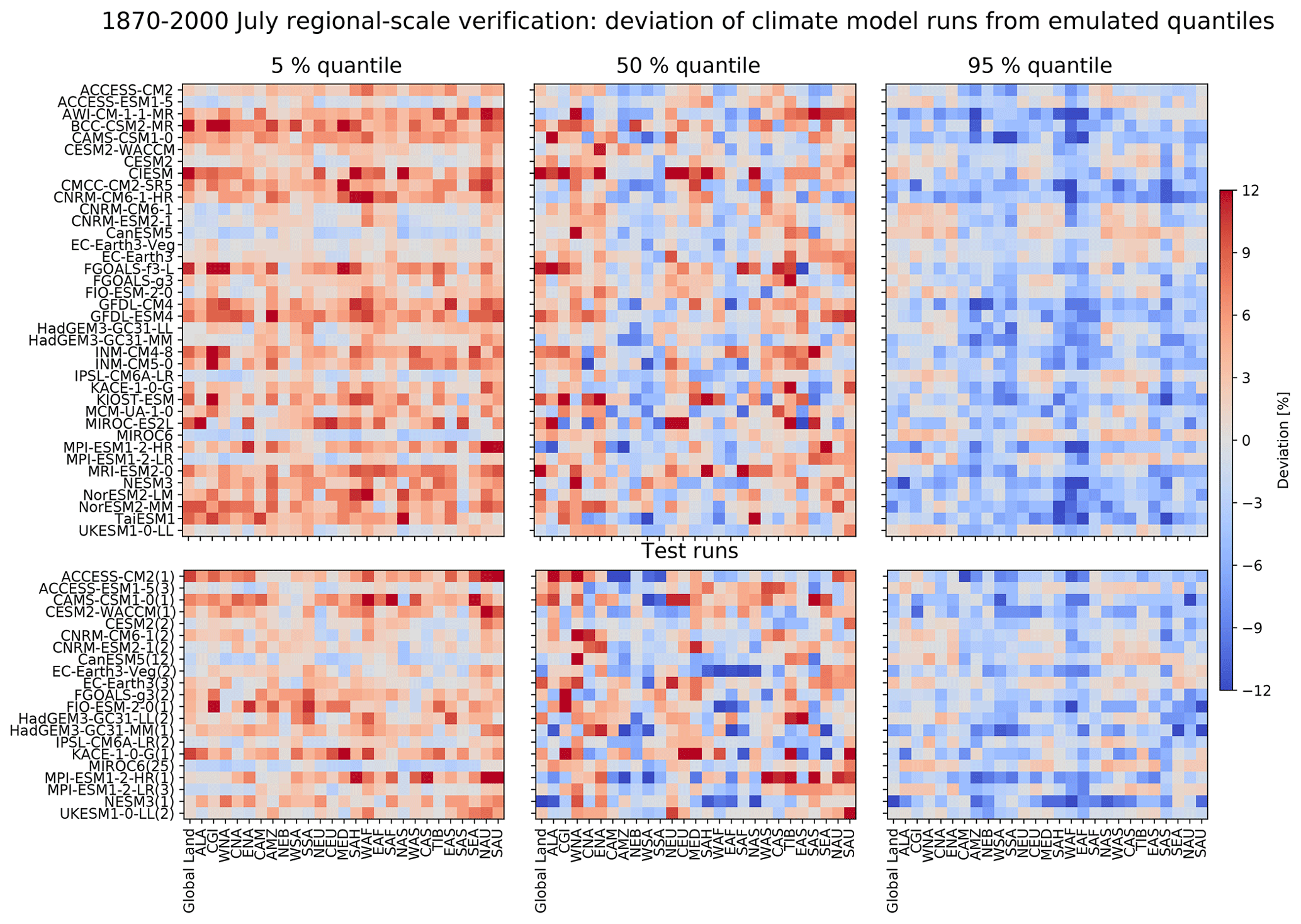

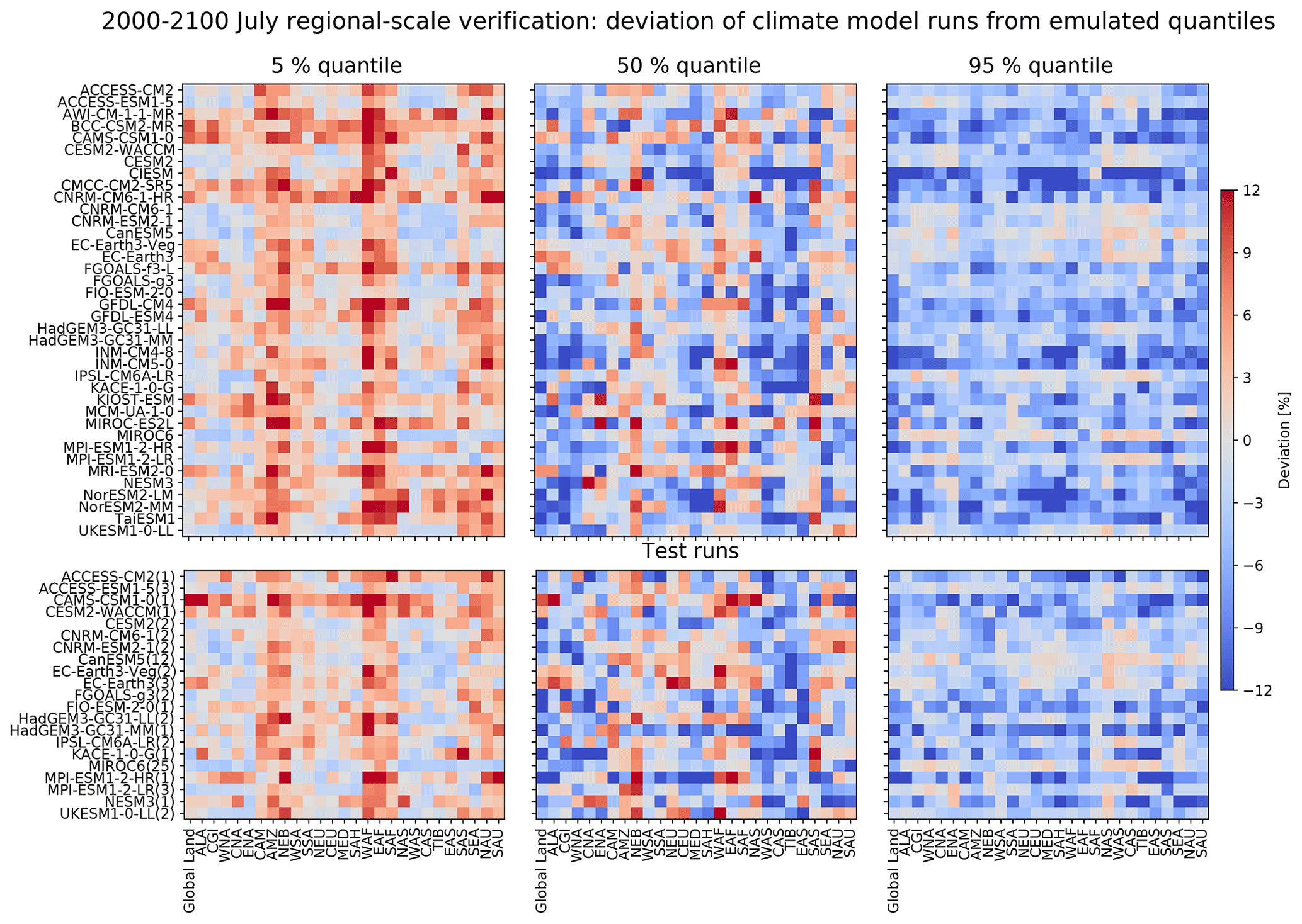
Generally, emulated 5 % (95 %) quantiles are warmer (colder) than those of the ESM training and test runs. Such under-dispersivity for regional averages is linked to the localization of the spatial covariance matrix within the residual variability module, such that spatial correlations drop faster within the emulator than they do in the actual ESM. For January over the time period of 1870–2000, the lowest magnitudes in 5 % and 95 % quantile deviations are observed for southern hemispheric regions (e.g. AMZ, NEB, WSA, SSA), along with slight over-dispersivity (see the blue 5 % quantile and red 95% quantile values in their respective panels of Fig. 8). Over the period of 2000–2100, this behaviour for January switches to northern hemispheric regions (e.g. CEU, ALA, ENA, WNA, TIB) and is mostly apparent for the 95 % quantile, possibly due to a decrease (increase) in January variability in the Northern (Southern) Hemisphere with increasing yearly temperatures (Holmes et al., 2016). In contrast, over both the periods of 1870–2000 and 2000–2100, July consistently displays the lowest magnitudes of 5 % and 95 % quantile deviations (even with a slight over-dispersivity) in northern hemispheric regions (e.g. WNA, ENA, NAS, WAS). The observed small regional over-dispersivities hint at additional processes being at play in these regions which are not accounted for by the emulator and that counteract the expected regional-scale under-dispersivity which is inherent in the emulator's residual variability module design.
5.4 Benchmarking MESMER-M using a simple physical approach
In-depth analysis of the benchmarking approach outlined in Sect. 3.3 is conducted for four selected ESMs which exhibit diverse genealogies (Knutti et al., 2013; Brunner et al., 2020) (see Fig. E1 for summarized results of all other ESMs). From Fig. 12, it is evident that adding even only one biophysical variable explains part of the residual difference behaviour, with correlations between the physically informed emulations and ESM runs (given relative to correlations between Tyr and “month” informed emulations and ESM runs) over global land always being positive. Across all four ESMs the main improvements are in northern hemispheric regions which possess distinct seasonal variations in snow cover namely, ALA, CGI, WNA, CNA, ENA, NEU, CEU, NAS, and CAS. MIROC6 and MPI-ESM1-2-LR exhibit substantial improvements in other regions, notably WAF, EAF, SAS and NAU regions. It is worth noting that for most ESMs, the biophysical predictor configuration of albedo, cloud cover, and snow cover (ACS) performs consistently worse than any configuration containing sensible and latent heat fluxes (H), suggesting the presence of processes only explainable using sensible and latent heat fluxes. MIROC6 is an exception to this, with both the biophysical configurations of latent heat flux (Hl) and H yielding 0 or lower relative correlations in WNA, CNA, ENA, CEU, and EAS, while HC (biophysical configuration of sensible heat fluxes, latent heat fluxes, and cloud cover) displays no improvements for these regions. This could be due to colinearities between cloud cover and latent and sensible heat fluxes alongside overfitting of the physically informed model to latent and sensible heat fluxes due to confounding variabilities.
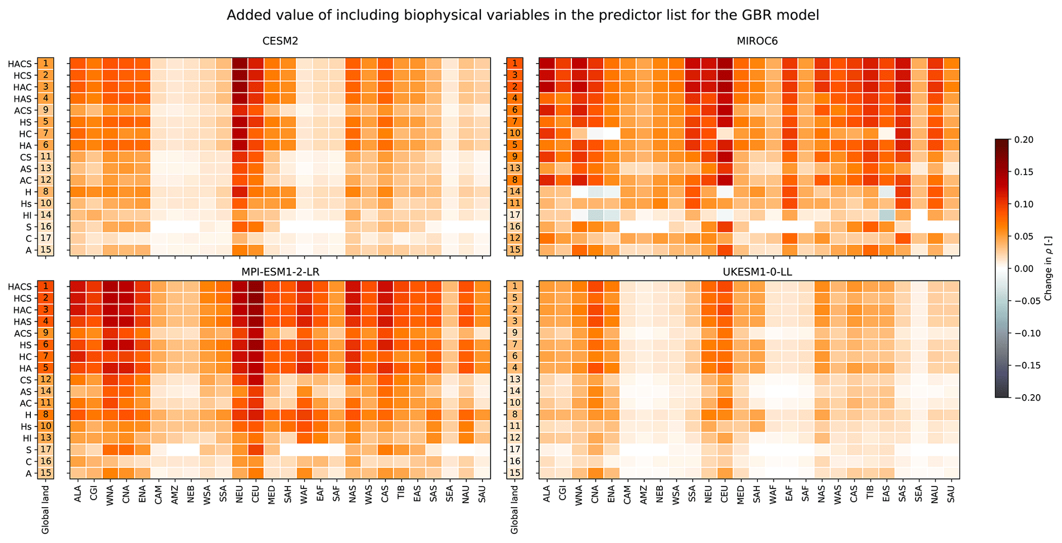
Figure 12Global land (without Antarctica) and regional performances (columns) of the physically informed model trained using different predictor sets (rows) shown for four selected CMIP6 models, for each SREX region. Acronyms for the predictor sets (y axis tick labels) can be referred back to in Table 1. Pearson correlations calculated over all months between test runs and harmonic-model test results augmented by the physically informed model's predictions of residual variability are considered. Here we show changes in correlations relative to those obtained when augmenting using only Tyr and month values as predictors. Numbers in the global land column indicate the ranking of each predictor set, where 1 is the best-performing.
As HACS (biophysical configuration of sensible heat fluxes, latent heat fluxes, albedo, cloud cover, and snow cover) performs the best globally (appears as 1 in global land) across all four ESMs, we choose it as the benchmark physically informed model to compare the residual variability module to. Figure 13 shows the energy distances of the physically informed (harmonic model+HACS) and statistical (full emulator = harmonic model + residual variability module) emulated cdfs to the ESM cdfs for January and July, where 0 indicates identical and thus “perfect” emulated cdfs. Energy distances in July for both the physically informed and statistical models are close to 0 indicating near-perfect cdfs, with only MIROC6 and MPI-ESM1-LR showing larger distances for the full emulator in the Indo-Gangetic region and central West Africa respectively. In contrast, January shows higher distances for both the physically informed and statistical model cdfs, particularly in northern hemispheric regions with seasonal snowfall and most notably in the full emulator of MIROC6. Overall, the statistical model performs better than the physically informed model for CESM2 and UKESM1-0-LL and worse for MIROC6 and MPI-ESM1-2-LR. An explanation behind this could the combination of biophysical feedbacks being more pronounced in January's northern hemispheric variability and that MIROC6 and MPI-ESM1-2-LR have at least four more training runs than CESM2 and UKESM1-0-LL, providing the GBR model with more training material to extract such biophysical information from. This suggests a limit to when the statistical approach performs better than the physical approach, depending on how present biophysical feedbacks are within the overall variability and how much information is available to train on. Nevertheless, without the prerequisite of having more training runs – which can be seen as an added advantage – the statistical approach taken by the full emulator generally shows better performances across most ESMs for January and July than the physical approach (Fig. E2). Thus, the distributional properties of local monthly temperatures as seen within ESM initial-condition ensembles can be sufficiently represented using the statistical approach outlined in this paper, which takes only local yearly temperatures as input.

Figure 13Comparison of the performance of the harmonic model + physically informed HACS model to that of the full emulator for January and July of four selected CMIP6 models. The energy distance from the actual model test runs is considered, where 0 indicates the best performance.
We extend MESMER's framework to include the monthly downscaling module, MESMER-M, trained for each ESM at each grid point individually, thus providing realistic, spatially explicit monthly temperature fields from yearly temperature fields in a matter of seconds. We assume a linear response of the seasonal temperature cycle to its yearly mean values and represent it using a harmonic model. Any remaining response patterns are expected to arise from regional-scale, physical, and intra-annual processes, such as snow–albedo feedbacks or the modulation of atmospheric circulation patterns due to changes in ENSO, and have asymmetric, non-uniform (i.e. non-linear, non-stationary, affecting variance and skewness) effects across months. To capture them, we build a month-specific residual variability module which samples spatio-temporally correlated terms, conserving lag-1 autocorrelations and spatial cross-correlations whilst accounting for specificities in the residual variability structure across months. By letting the skewness of the residual sampling space additionally covary with yearly temperatures, non-uniformities in secondary feedbacks are furthermore inferred through their manifestations within the monthly temperature distributions.
Verification results across all ESMs show the emulator altogether reproducing the mean monthly temperature response, as well as conserving temporal and spatial correlation patterns and regional-scale temperature distributions up to a degree sensible to its simplicity. To further assess how well the emulator is able to represent non-uniformities in the monthly temperature response arising from secondary biophysical feedbacks, we compare its performance to that of a simple physically informed model built on biophysical information. The emulator overall reproduces the cdfs of the actual ESM just as well as, and in most cases even better than, the physically informed model, evidencing the validity of such a statistical approach in inferring temperature distributions and thus the uncertainty due to natural variability within temperature realizations. Given that the uncertainty due to natural variability is a property intrinsic to climate models and largely irreducible (Deser et al., 2020), the emulator thus proves itself as a pragmatic alternative to otherwise having to generate large single-model, initial-condition ensembles.
6.1 Further emulator developments
In this study, MESMER-M was only trained on SSP5-8.5 climate scenario runs so as to demonstrate its performance over the extreme spectrum of climate response types. A further step would be to investigate the inter-scenario applicability of MESMER-M, and this has already been done for MESMER with satisfactory results (Beusch et al., 2022). While we would expect the overall mean response of monthly to yearly temperatures to remain relatively stable between climate scenarios, non-uniformities arising in the local variability may be more scenario-specific (e.g. due to slowing down of the snow–albedo feedback under an equilibrated climate for low-emission scenarios). Bearing this in mind, we recommend training MESMER-M on all available climate scenarios before using it for inter-scenario exploration. Such would provide the local Yeo–Johnson transformation with enough information on the relationship between yearly temperatures and skewness of monthly temperatures. Additional adjustments such as considering the rate of yearly temperature change as a covariate to monthly temperature skewness could also be investigated.
This study demonstrates the advantage of constructing modular emulators such that the emulator framework can be extended according to the area of application. Additional module developments which increase the impact relevance of the emulations and improve the fidelity in global and regional representation of monthly temperatures under different climate scenarios should be given priority. A module that comes to mind would be one representing changes in land cover, such as de/afforestation, which has been historically assessed to have biophysical impacts of a similar magnitude on regional climate as the concomitant increase in GHGs (De Noblet-Ducoudré et al., 2012) and for which very distinct imprints on the seasonal cycle of temperatures as well as the tails of the temperature distributions have been identified (Pitman et al., 2012; Lejeune et al., 2017). Such a module would furthermore increase the emulator's relevance towards impact assessments, in light of the important land cover changes expected to happen in the 21st century (Popp et al., 2017; O'Neill et al., 2016) and the relevance of accounting for their regional climate impacts especially in high-mitigation scenarios such as those compatible with the 1.5 ∘C long-term temperature goal of the Paris Agreement (Seneviratne et al., 2018; Roe et al., 2019; Arneth et al., 2019)). One technical advantage of adding a land cover module would be that the effect of land cover changes can be expected to be sufficiently decoupled from the overall GHG-induced temperature response (De Noblet-Ducoudré et al., 2012; Lejeune et al., 2017). Hence, the direct local effect of such a module would not interfere with the mean temperature response as extracted within the rest of the emulator.
Another modular development could include an explicit representation of the main modes of climate variability, such as ENSO, so as to strengthen MESMER-M's inter-annual variability representation. Since these modes are potentially coupled to the overall GHG-induced temperature response however, such an inclusion would be more complicated. One possible approach could be to introduce soil moisture as an additional variable term and investigate its lag correlations to monthly temperature variabilities. Alternatively we could explore building upon existing approaches such as the one of McKinnon and Deser (2018). Bearing in mind that one key advantage of MESMER-M is that it only requires yearly temperatures as input, the added value of such a module should be critically assessed against the need for additional predictors. Another possibility could be to instead decompose the covariance matrix used in (see Fig. 1) so as to account for spatial cross-correlations affected by major modes of variability; however, in this case the added model complexity should again be weighed against gained skill in emulation.
6.2 Potential further applications of the GBR-based physically informed approach
Beusch et al. (2020) pointed out that the ESM-specific emulator calibration results represent distinct “model IDs”, containing scale-dependent information of the model structure. As a follow-up from the physically informed model-based benchmarking done within this study, we further propose that the residuals from the mean response module also contain ESM-specific, scale-dependent information, constituting the distinct representations and parameterizations of biophysical feedbacks within each ESM. For example, models with strong snow–albedo feedbacks and a large snow cover reduction with increasing global mean temperature will show stronger warming of cold months (Fischer et al., 2011) and thus more negatively skewed residuals for those months. A step towards disentangling such process representation within the ESMs has already been made in this study, through the representation of biophysical contributions within residual variabilities using the GBR-based physically informed model. Further analysing the strength of the covariations in different biophysical variables with the residuals, as identified by the physically informed model, could then help isolate the exact contributions of these variables. While the key physical variables contributing to temperature variability within ESMs have already been studied (Schwingshackl et al., 2018), such an analysis would further provide information on the amount by which a selected number of biophysical variables contribute to residual variability within each ESM. Performing a similar analysis on observational datasets and comparing the results to those of the ESMs could then serve as a means to evaluate model representation of biophysical interactions under a changing climate.
Table A1List of the 38 employed CMIP6 models, the modelling groups providing them, and the number of initial-condition ensemble members used in the training and test sets.


Figure B1Shapiro–Wilk test for normality of January temperature residuals. The null hypothesis is that the residuals are normally distributed. A Benjamini–Hochberg multiple test correction (Benjamini and Hochberg, 1995) is applied to the p values before plotting them. Percentage values indicate the proportion of grid points for which the null hypothesis is rejected.

Figure B2Same as Fig. B1, except for July.
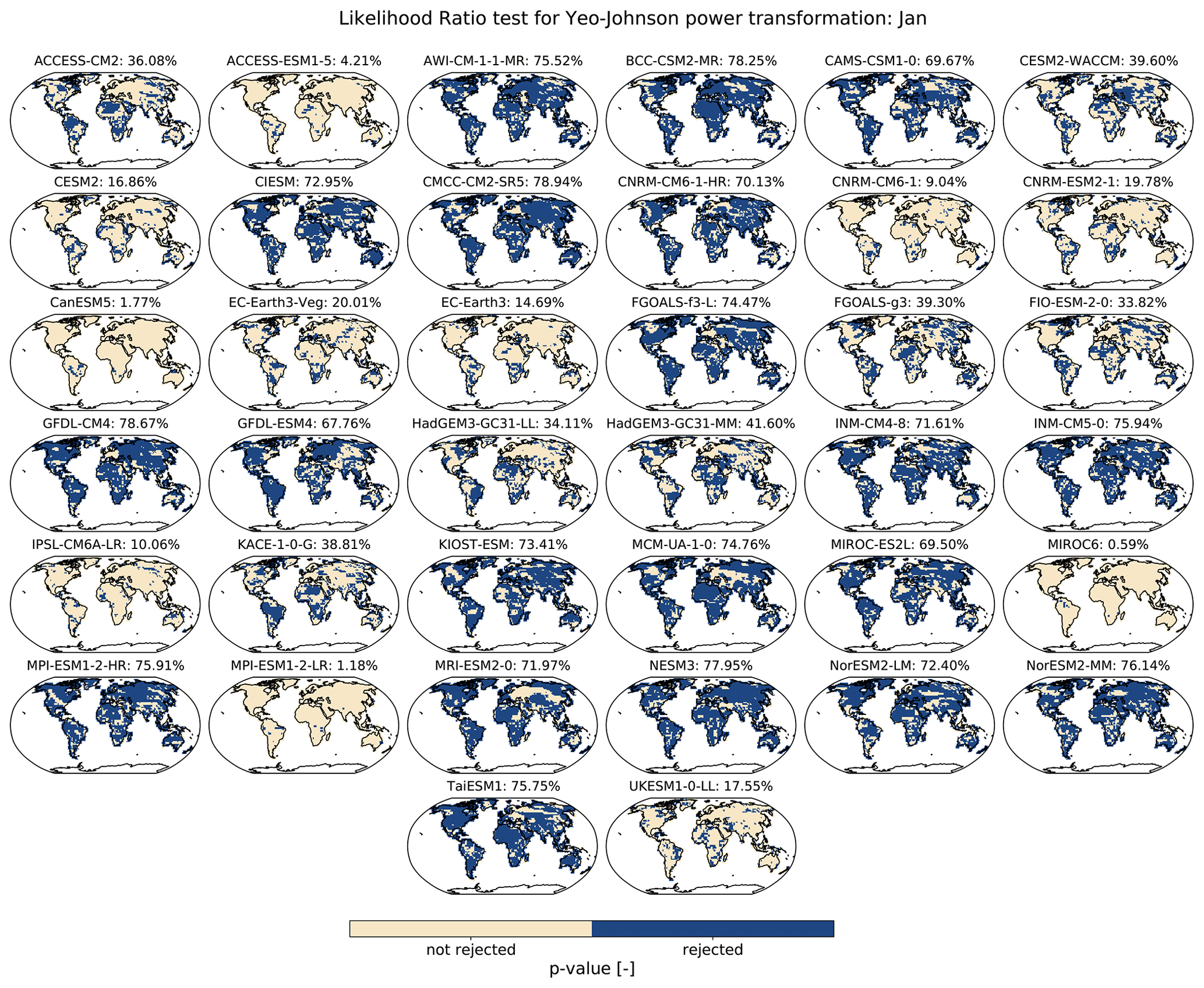
Figure C1Likelihood ratio test comparing the performance of January's Yeo–Johnson transformations when using just one single lambda parameter (λm,s) vs. when using a yearly temperature-dependent lambda parameter (). The null hypothesis is that the λm,s-based transformation performs better than the -based transformation. A Benjamini–Hochberg multiple test correction (Benjamini and Hochberg, 1995) is applied to the p values before plotting them. Percentage values indicate the proportion of grid points for which the null hypothesis is rejected.
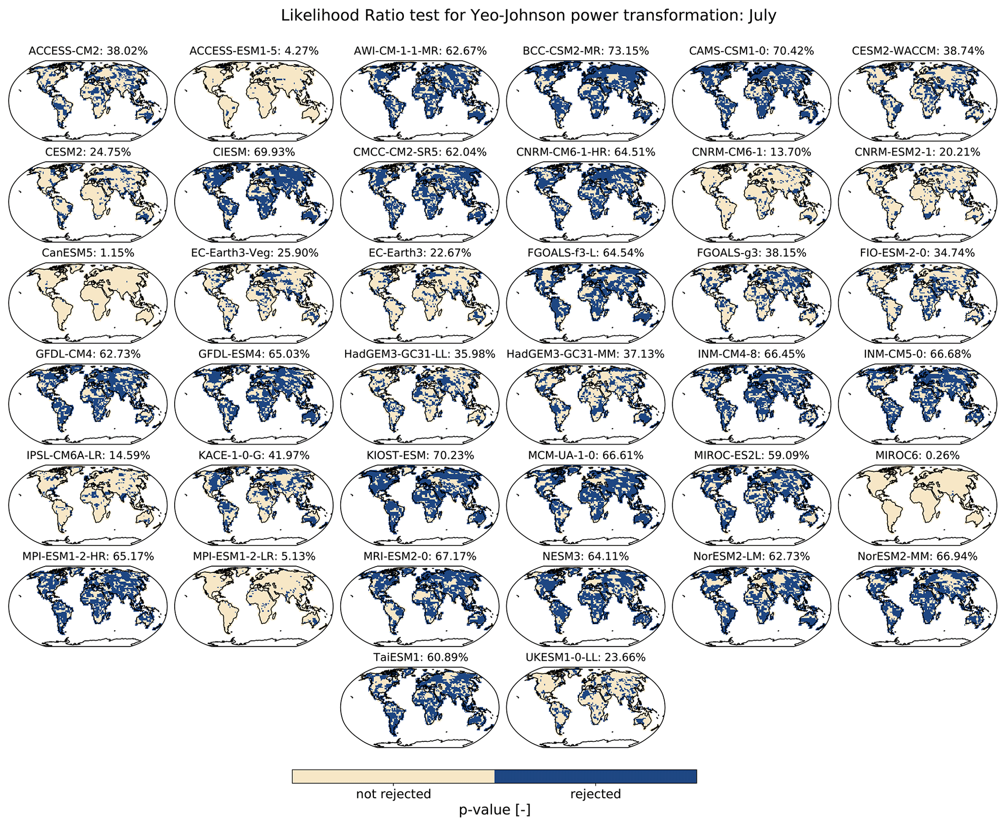
Figure C2Same as Fig. C1, except for July.
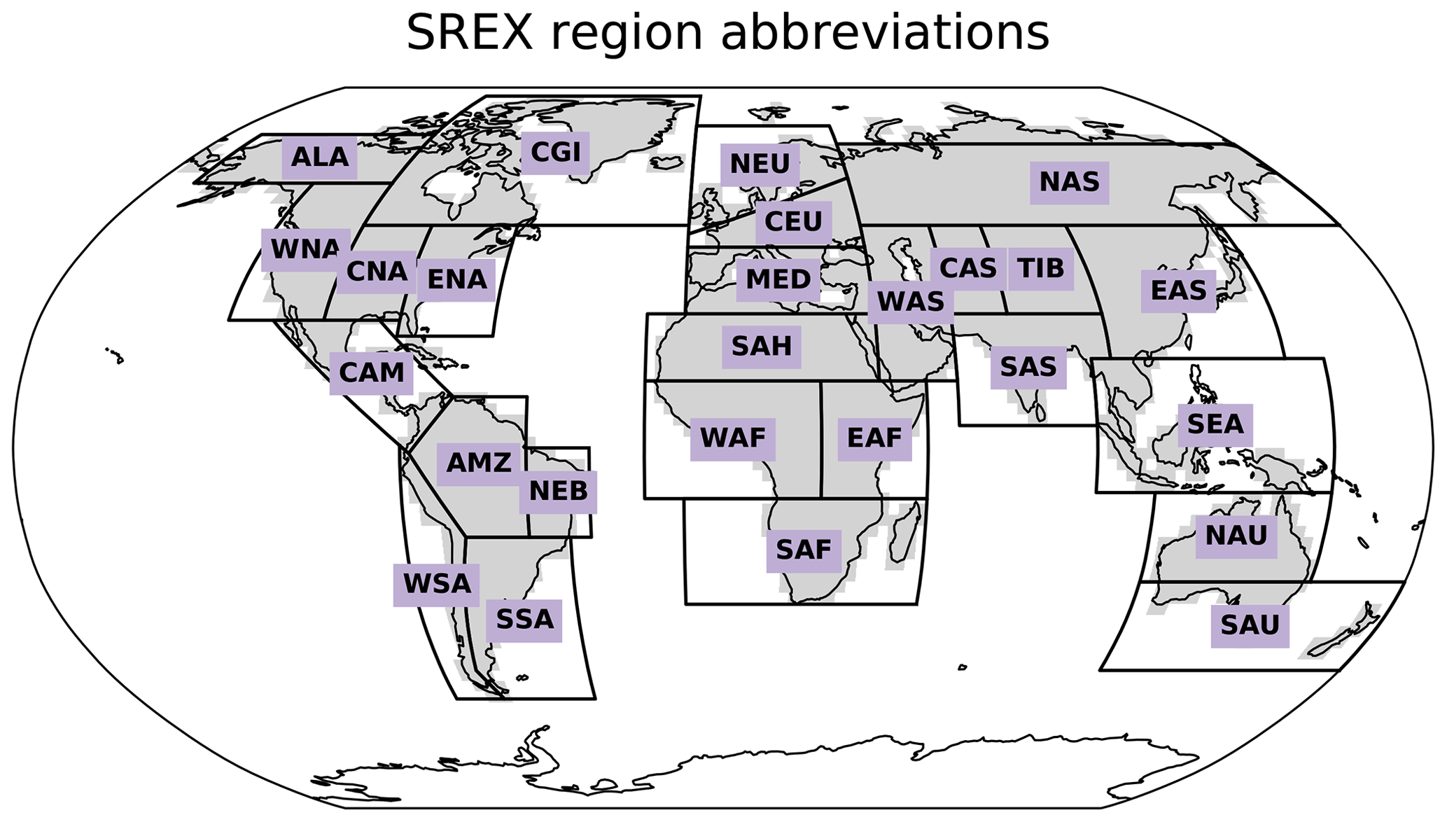
Figure D1Map of the SREX regions and their abbreviations. The considered land grid points are shown in grey.

Figure E1Same as Fig. 12, except that all CMIP6 models are shown for the global land (without Antarctica).
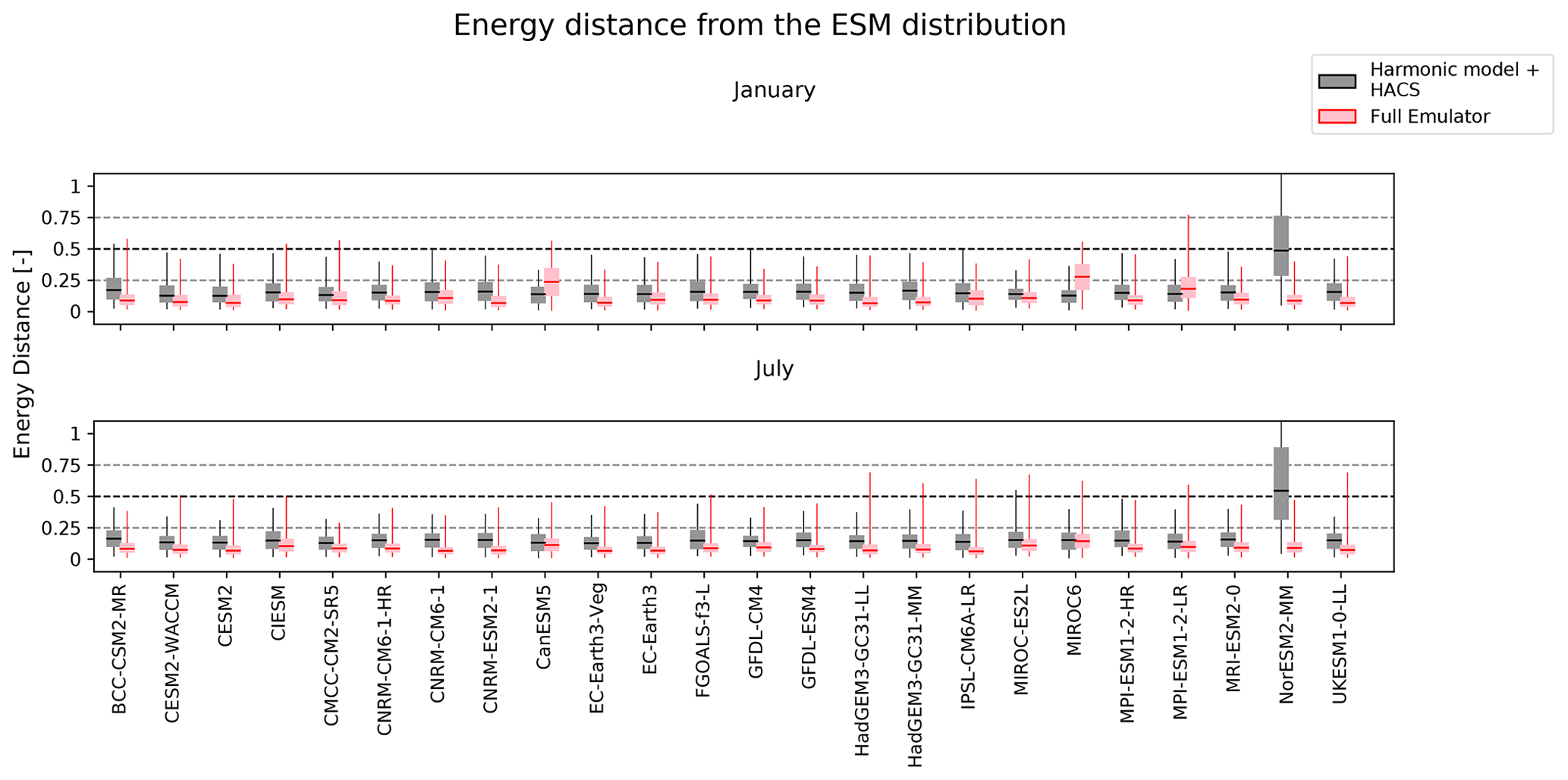
Figure E2Comparison of the performance of the harmonic model + physically informed HACS model to that of the full emulator for January and July of all CMIP6 models. The energy distance from the actual model test runs is considered, where 0 indicates the best performance. Boxplot whiskers indicate 5th and 95th quantiles.
The original MESMER is publicly available on GitHub (https://doi.org/10.5281/zenodo.5106843, Hauser et al., 2021) with documentation hosted on Read the Docs (https://mesmer-emulator.readthedocs.io/en/stable/, last access: 22 April 2022). Harmonization of the MESMER-M code onto the GitHub page is still in progress. MESMER-M code in its current state and scripts for the analysis and plotting done within this paper are additionally archived on Zenodo (https://doi.org/10.5281/zenodo.6477493, Nath, 2022).
The CMIP6 data are available from the public CMIP archive at https://esgf-node.llnl.gov/projects/esgf-llnl/ (ESGF-LNLL, 2022).
QL, CFS, and SIS identified the need to extend MESMER's framework by a monthly downscaling module. SN designed the monthly downscaling module with support and guidance from QL and LB. SN led the analysis and drafted the text with help from QL in developing the storyline. All authors contributed to interpreting results and streamlining the text.
The contact author has declared that neither they nor their co-authors have any competing interests.
Publisher's note: Copernicus Publications remains neutral with regard to jurisdictional claims in published maps and institutional affiliations.
We thank Lukas Gudmundsson, Joel Zeder, and Christoph Frei for their invaluable statistical insight into the development and analysis of the emulator modules. Finally, we thank the climate modelling groups listed in Table A1 for producing and making available the CMIP6 model outputs and Urs Beyerle and Lukas Brunner for downloading the CMIP6 data and pre-processing them.
This research has been supported by the Bundesministerium für Bildung und Forschung and the Deutsches Zentrum für Luft- und Raumfahrt as part of AXIS, an ERANET initiated by JPI Climate (grant no. 01LS1905A), the European Commission, Horizon 2020 Framework Programme (AXIS (grant no. 776608)), and the European Research Council, H2020 (MESMER-X (grant no. 964013)).
This paper was edited by Gabriele Messori and reviewed by three anonymous referees.
Alexeeff, S. E., Nychka, D., Sain, S. R., and Tebaldi, C.: Emulating mean patterns and variability of temperature across and within scenarios in anthropogenic climate change experiments, Climatic Change, 146, 319–333, https://doi.org/10.1007/s10584-016-1809-8, 2018. a, b
Allen, R. J. and Zender, C. S.: Forcing of the Arctic Oscillation by Eurasian snow cover, J. Climate, 24, 6528–6539, https://doi.org/10.1175/2011JCLI4157.1, 2011. a
Arneth, A., Barbosa, H., Benton, T., Calvin, K., Calvo, E., Connors, S., Cowie, A., Davin, E., Denton, F., van Diemen, R., Driouech, F., Elbehri, A., Evans, J., Ferrat, M., Harold, J., Haughey, E., Herrero, M., House, J., Howden, M., Hurlbert, M., Jia, G., Gabriel, T. J., Krishnaswamy, J., Kurz, W., Lennard, C., Myeong, S., Mahmoud, N., Delmotte, V. M., Mbow, C., McElwee, P., Mirzabaev, A., Morelli, A., Moufouma-Okia, W., Nedjraoui, D., Neogi, S., Nkem, J., Noblet-Ducoudré, N. D., Pathak, L. O. M., Petzold, J., Pichs-Madruga, R., Poloczanska, E., Popp, A., Pörtner, H.-O., Pereira, J. P., Pradhan, P., Reisinger, A., Roberts, D. C., Rosenzweig, C., Rounsevell, M., Shevliakova, E., Shukla, P., Skea, J., Slade, R., Smith, P., Sokona, Y., Sonwa, D. J., Soussana, J.-F., Tubiello, F., Verchot, L., Warner, K., Weyer, N., Wu, J., Yassaa, N., Zhai, P., and Zommers, Z.: IPCC SR: Climate Change and Land, An IPCC Special Report on climate change, desertification, land degradation, sustainable land management, food security, and greenhouse gas fluxes in terrestrial ecosystems, p. 43, in press, 2019. a
Arnold, L.: Hasselmann's program revisited: the analysis of stochasticity in deterministic climate models, in: Stochastic Climate Models, edited by: Imkeller, P. and von Storch, J.-S., Birkhäuser Basel, Basel, 141–157, https://doi.org/10.1007/978-3-0348-8287-3_5, 2001. a
Benjamini, Y. and Hochberg, Y.: benjamini_hochberg1995, J. Roy. Stat. Soc. B, 57, 289–300, 1995. a, b
Berner, J., Achatz, U., Batté, L., Bengtsson, L., De La Cámara, A., Christensen, H. M., Colangeli, M., Coleman, D. R., Crommelin, D., Dolaptchiev, S. I., Franzke, C. L., Friederichs, P., Imkeller, P., Järvinen, H., Juricke, S., Kitsios, V., Lott, F., Lucarini, V., Mahajaajaajan, S., Palmer, T. N., Penland, C., Sakradzijaja, M., Von Storch, J. S., Weisheimer, A., Weniger, M., Williams, P. D., and Yano, J. I.: Stochastic parameterization toward a new view of weather and climate models, B. Am. Meteorol. Soc., 98, 565–587, https://doi.org/10.1175/BAMS-D-15-00268.1, 2017. a
Beusch, L., Gudmundsson, L., and Seneviratne, S. I.: Emulating Earth system model temperatures with MESMER: from global mean temperature trajectories to grid-point-level realizations on land, Earth Syst. Dynam., 11, 139–159, https://doi.org/10.5194/esd-11-139-2020, 2020. a, b, c, d, e, f, g, h, i, j
Beusch, L., Nicholls, Z., Gudmundsson, L., Hauser, M., Meinshausen, M., and Seneviratne, S. I.: From emission scenarios to spatially resolved projections with a chain of computationally efficient emulators: coupling of MAGICC (v7.5.1) and MESMER (v0.8.3), Geosci. Model Dev., 15, 2085–2103, https://doi.org/10.5194/gmd-15-2085-2022, 2022. a
Blackport, R. and Kushner, P. J.: The transient and equilibrium climate response to rapid summertime sea ice loss in CCSM4, J. Climate, 29, 401–417, https://doi.org/10.1175/JCLI-D-15-0284.1, 2016. a
Brunner, L., Pendergrass, A. G., Lehner, F., Merrifield, A. L., Lorenz, R., and Knutti, R.: Reduced global warming from CMIP6 projections when weighting models by performance and independence, Earth Syst. Dynam., 11, 995–1012, https://doi.org/10.5194/esd-11-995-2020, 2020. a, b
Castruccio, S., Hu, Z., Sanderson, B., Karspeck, A., and Hammerling, D.: Reproducing internal variability with few ensemble runs, J. Climate, 32, 8511–8522, https://doi.org/10.1175/JCLI-D-19-0280.1, 2019. a, b
Cohen, J. and Rind, D.: The Effect of Snow Cover on the Climate, J. Climate, 4, 689–706, https://doi.org/10.1175/1520-0442(1991)004<0689:TEOSCO>2.0.CO;2, 1991. a, b
Colman, R. A.: Surface albedo feedbacks from climate variability and change, J. Geophys. Res.-Atmos., 118, 2827–2834, https://doi.org/10.1002/jgrd.50230, 2013. a, b
De Noblet-Ducoudré, N., Boisier, J. P., Pitman, A., Bonan, G. B., Brovkin, V., Cruz, F., Delire, C., Gayler, V., Van Den Hurk, B. J., Lawrence, P. J., Van Der Molen, M. K., Müller, C., Reick, C. H., Strengers, B. J., and Voldoire, A.: Determining robust impacts of land-use-induced land cover changes on surface climate over North America and Eurasia: Results from the first set of LUCID experiments, J. Climate, 25, 3261–3281, https://doi.org/10.1175/JCLI-D-11-00338.1, 2012. a, b
Deser, C., Phillips, A. S., Tomas, R. A., Okumura, Y. M., Alexander, M. A., Capotondi, A., Scott, J. D., Kwon, Y. O., and Ohba, M.: ENSO and pacific decadal variability in the community climate system model version 4, J. Climate, 25, 2622–2651, https://doi.org/10.1175/JCLI-D-11-00301.1, 2012. a
Deser, C., Lehner, F., Rodgers, K. B., Ault, T., Delworth, T. L., DiNezio, P. N., Fiore, A., Frankignoul, C., Fyfe, J. C., Horton, D. E., Kay, J. E., Knutti, R., Lovenduski, N. S., Marotzke, J., McKinnon, K. A., Minobe, S., Randerson, J., Screen, J. A., Simpson, I. R., and Ting, M.: Insights from Earth system model initial-condition large ensembles and future prospects, Nat. Clim. Change, 10, 277–286, https://doi.org/10.1038/s41558-020-0731-2, 2020. a
ESGF-LNLL: ESGF@DOE/LLNL, https://esgf-node.llnl.gov/projects/esgf-llnl/, last access: 22 April 2022. a
Eyring, V., Bony, S., Meehl, G. A., Senior, C. A., Stevens, B., Stouffer, R. J., and Taylor, K. E.: Overview of the Coupled Model Intercomparison Project Phase 6 (CMIP6) experimental design and organization, Geosci. Model Dev., 9, 1937–1958, https://doi.org/10.5194/gmd-9-1937-2016, 2016. a
Fischer, E. M., Lawrence, D. M., and Sanderson, B. M.: Quantifying uncertainties in projections of extremes-a perturbed land surface parameter experiment, Clim. Dynam., 37, 1381–1398, https://doi.org/10.1007/s00382-010-0915-y, 2011. a, b
Fischer, E. M., Rajczak, J., and Schär, C.: Changes in European summer temperature variability revisited, Geophys. Res. Lett., 39, 1–8, https://doi.org/10.1029/2012GL052730, 2012. a
Frei, C. and Isotta, F. A.: Ensemble Spatial Precipitation Analysis From Rain Gauge Data: Methodology and Application in the European Alps, J. Geophys. Res.-Atmos., 124, 5757–5778, https://doi.org/10.1029/2018JD030004, 2019. a
Gaspari, G. and Cohn, S. E.: Construction of correlation functions in two and three dimensions, Q. J. Roy. Meteorol. Soc., 125, 723–757, https://doi.org/10.1256/smsqj.55416, 1999. a
Hall, A.: The role of surface albedo feedback in climate, J. Climate, 17, 1550–1568, https://doi.org/10.1175/1520-0442(2004)017<1550:TROSAF>2.0.CO;2, 2004. a, b
Hastie, T., Tibshirani, R., and Friedman, J.: Elements of Statistical Learning, Ed. 2, Springer, ISBN 978-0-387-84858-7, 2009. a
Hauser, M., Beusch, L., Nicholls, Z., and woodhome23: MESMER-group/mesmer: version 0.8.3 (v0.8.3), Zenodo [code], https://doi.org/10.5281/zenodo.5106843, 2021. a
Holmes, C. R., Woollings, T., Hawkins, E., and de Vries, H.: Robust future changes in temperature variability under greenhouse gas forcing and the relationship with thermal advection, J. Climate, 29, 2221–2236, https://doi.org/10.1175/JCLI-D-14-00735.1, 2016. a, b
Huntingford, C., Jones, P. D., Livina, V. N., Lenton, T. M., and Cox, P. M.: No increase in global temperature variability despite changing regional patterns, Nature, 500, 327–330, https://doi.org/10.1038/nature12310, 2013. a
Jaeger, E. B. and Seneviratne, S. I.: Impact of soil moisture-atmosphere coupling on European climate extremes and trends in a regional climate model, Clim. Dynam., 36, 1919–1939, https://doi.org/10.1007/s00382-010-0780-8, 2011. a
King, A. D.: The drivers of nonlinear local temperature change under global warming, Environ. Res. Lett., 14, 064005, https://doi.org/10.1088/1748-9326/ab1976, 2019. a
Knutti, R., Masson, D., and Gettelman, A.: Climate model genealogy: Generation CMIP5 and how we got there, Geophys. Res. Lett., 40, 1194–1199, https://doi.org/10.1002/grl.50256, 2013. a
Lejeune, Q., Seneviratne, S. I., and Davin, E. L.: Historical land-cover change impacts on climate: Comparative assessment of LUCID and CMIP5 multimodel experiments, J. Climate, 30, 1439–1459, https://doi.org/10.1175/JCLI-D-16-0213.1, 2017. a, b
Link, R., Snyder, A., Lynch, C., Hartin, C., Kravitz, B., and Bond-Lamberty, B.: Fldgen v1.0: An emulator with internal variability and space-Time correlation for Earth system models, Geosci. Model Dev., 12, 1477–1489, https://doi.org/10.5194/gmd-12-1477-2019, 2019. a, b
Loikith, P. C. and Neelin, J. D.: Non-Gaussian cold-side temperature distribution tails and associated synoptic meteorology, J. Climate, 32, 8399–8414, https://doi.org/10.1175/JCLI-D-19-0344.1, 2019. a
Matalas, N. C.: Mathematical assessment of synthetic hydrology, Water Resour. Res., 3, 937–945, https://doi.org/10.1029/WR003i004p00937, 1967. a
McKinnon, K. A. and Deser, C.: Internal variability and regional climate trends in an observational large ensemble, J. Climate, 31, 6783–6802, https://doi.org/10.1175/JCLI-D-17-0901.1, 2018. a, b
Meinshausen, M., Raper, S. C., and Wigley, T. M.: Emulating coupled atmosphere-ocean and carbon cycle models with a simpler model, MAGICC6 – Part 1: Model description and calibration, Atmos. Chem. Phys., 11, 1417–1456, https://doi.org/10.5194/acp-11-1417-2011, 2011. a
Nath, S.: snath-xoc/Nath_et_al_ESD_2022_MESMER-M (v0.0.1), Zenodo [code], https://doi.org/10.5281/zenodo.6477493, 2022. a
Neale, R. B., Richter, J. H., and Jochum, M.: The impact of convection on ENSO: From a delayed oscillator to a series of events, J. Climate, 21, 5904–5924, https://doi.org/10.1175/2008JCLI2244.1, 2008. a
O'Neill, B. C., Tebaldi, C., Van Vuuren, D. P., Eyring, V., Friedlingstein, P., Hurtt, G., Knutti, R., Kriegler, E., Lamarque, J. F., Lowe, J., Meehl, G. A., Moss, R., Riahi, K., and Sanderson, B. M.: The Scenario Model Intercomparison Project (ScenarioMIP) for CMIP6, Geosci. Model Dev., 9, 3461–3482, https://doi.org/10.5194/gmd-9-3461-2016, 2016. a, b
Osborn, T. J., Wallace, C. J., Harris, I. C., and Melvin, T. M.: Pattern scaling using ClimGen: monthly-resolution future climate scenarios including changes in the variability of precipitation, Climatic Change, 134, 353–369, https://doi.org/10.1007/s10584-015-1509-9, 2016. a
Pitman, A. J., de Noblet-Ducoudré, N., Avila, F. B., Alexander, L. V., Boisier, J.-P., Brovkin, V., Delire, C., Cruz, F., Donat, M. G., Gayler, V., van den Hurk, B., Reick, C., and Voldoire, A.: Effects of land cover change on temperature and rainfall extremes in multi-model ensemble simulations, Earth Syst. Dynam., 3, 213–231, https://doi.org/10.5194/esd-3-213-2012, 2012. a
Popp, A., Calvin, K., Fujimori, S., Havlik, P., Humpenöder, F., Stehfest, E., Bodirsky, B. L., Dietrich, J. P., Doelmann, J. C., Gusti, M., Hasegawa, T., Kyle, P., Obersteiner, M., Tabeau, A., Takahashi, K., Valin, H., Waldhoff, S., Weindl, I., Wise, M., Kriegler, E., Lotze-Campen, H., Fricko, O., Riahi, K., and van Vuuren, D. P.: Land-use futures in the shared socio-economic pathways, Global Environ. Change, 42, 331–345, https://doi.org/10.1016/j.gloenvcha.2016.10.002, 2017. a
Potopová, V., Boroneanţ, C., Možný, M., and Soukup, J.: Driving role of snow cover on soil moisture and drought development during the growing season in the Czech Republic, Int. J. Climatol., 36, 3741–3758, https://doi.org/10.1002/joc.4588, 2016. a
Richardson, C. W.: Stochastic simulation of daily precipitation, temperature, and solar radiation, Water Resour. Res., 17, 182–190, https://doi.org/10.1029/WR017i001p00182, 1981. a
Roe, S., Streck, C., Obersteiner, M., Frank, S., Griscom, B., Drouet, L., Fricko, O., Gusti, M., Harris, N., Hasegawa, T., Hausfather, Z., Havlík, P., House, J., Nabuurs, G. J., Popp, A., Sánchez, M. J. S., Sanderman, J., Smith, P., Stehfest, E., and Lawrence, D.: Contribution of the land sector to a 1.5 ∘C world, Nat. Clim. Change, 9, 817–828, https://doi.org/10.1038/s41558-019-0591-9, 2019. a
Schlenker, W. and Roberts, M. J.: Nonlinear temperature effects indicate severe damages to U.S. crop yields under climate change, P. Natl. Acad. Sci. USA, 106, 15594–15598, https://doi.org/10.1073/pnas.0906865106, 2009. a
Schwingshackl, C., Hirschi, M., and Seneviratne, S. I.: Global Contributions of Incoming Radiation and Land Surface Conditions to Maximum Near-Surface Air Temperature Variability and Trend, Geophys. Res. Lett., 45, 5034–5044, https://doi.org/10.1029/2018GL077794, 2018. a
Seneviratne, S. I., Nicholls, N., Easterling, D., Goodess, C. M., Kanae, S., Kossin, J., Luo, Y., Marengo, J., Mc Innes, K., Rahimi, M., Reichstein, M., Sorteberg, A., Vera, C., Zhang, X., Rusticucci, M., Semenov, V., Alexander, L. V., Allen, S., Benito, G., Cavazos, T., Clague, J., Conway, D., Della-Marta, P. M., Gerber, M., Gong, S., Goswami, B. N., Hemer, M., Huggel, C., Van den Hurk, B., Kharin, V. V., Kitoh, A., Klein Tank, A. M., Li, G., Mason, S., Mc Guire, W., Van Oldenborgh, G. J., Orlowsky, B., Smith, S., Thiaw, W., Velegrakis, A., Yiou, P., Zhang, T., Zhou, T., and Zwiers, F. W.: Changes in climate extremes and their impacts on the natural physical environment, in: Managing the Risks of Extreme Events and Disasters to Advance Climate Change Adaptation: Special Report of the Intergovernmental Panel on Climate Change, edited by: Field, C., Barros, V., Stocker, T., and Dahe, Q., Cambridge University Press, 9781107025, 109–230, https://doi.org/10.1017/CBO9781139177245.006, 2012. a
Seneviratne, S. I., Wartenburger, R., Guillod, B. P., Hirsch, A. L., Vogel, M. M., Brovkin, V., Van Vuuren, D. P., Schaller, N., Boysen, L., Calvin, K. V., Doelman, J., Greve, P., Havlik, P., Humpenöder, F., Krisztin, T., Mitchell, D., Popp, A., Riahi, K., Rogelj, J., Schleussner, C. F., Sillmann, J., and Stehfest, E.: Climate extremes, land-climate feedbacks and land-use forcing at 1.5 ∘C, Philos. T. Roy. Soc. A, 376, 20160450, https://doi.org/10.1098/rsta.2016.0450, 2018. a
Sheridan, S. C. and Lee, C. C.: Temporal Trends in Absolute and Relative Extreme Temperature Events Across North America, J. Geophys. Res.-Atmos., 123, 11889–11898, https://doi.org/10.1029/2018JD029150, 2018. a, b
Stéfanon, M., Drobinski, P., D'Andrea, F., and De Noblet-Ducoudré, N.: Effects of interactive vegetation phenology on the 2003 summer heat waves, J. Geophys. Res.-Atmos., 117, 1–15, https://doi.org/10.1029/2012JD018187, 2012. a
Tamarin-Brodsky, T., Hodges, K., Hoskins, B. J., and Shepherd, T. G.: Changes in Northern Hemisphere temperature variability shaped by regional warming patterns, Nat. Geosci., 13, 414–421, https://doi.org/10.1038/s41561-020-0576-3, 2020. a, b, c
Tebaldi, C. and Arblaster, J. M.: Pattern scaling: Its strengths and limitations, and an update on the latest model simulations, Climatic Change, 122, 459–471, https://doi.org/10.1007/s10584-013-1032-9, 2014. a, b
Thackeray, C. W., Derksen, C., Fletcher, C. G., and Hall, A.: Snow and Climate: Feedbacks, Drivers, and Indices of Change, Curr. Clim. Change Rep., 5, 322–333, https://doi.org/10.1007/s40641-019-00143-w, 2019. a, b
Thompson, D. W., Barnes, E. A., Deser, C., Foust, W. E., and Phillips, A. S.: Quantifying the role of internal climate variability in future climate trends, J. Climate, 28, 6443–6456, https://doi.org/10.1175/JCLI-D-14-00830.1, 2015. a
Wang, Z., Jiang, Y., Wan, H., Yan, J., and Zhang, X.: Detection and attribution of changes in extreme temperatures at regional scale, J. Climate, 30, 7035–7047, https://doi.org/10.1175/JCLI-D-15-0835.1, 2017. a, b
Wramneby, A., Smith, B., and Samuelsson, P.: Hot spots of vegetation-climate feedbacks under future greenhouse forcing in Europe, J. Geophys. Res.-Atmos., 115, 1–12, https://doi.org/10.1029/2010JD014307, 2010. a
Xu, L. and Dirmeyer, P.: Snow-atmosphere coupling strength in a global atmospheric model, Geophys. Res. Lett., 38, 1–5, https://doi.org/10.1029/2011GL048049, 2011. a
Yeo, I.-K. and Johnson, R. A.: A New Family of Power Transformations to Improve Normality or Symmetry, Biometrika, 87, 954–959, 2000. a, b
Zhao, C., Liu, B., Piao, S., Wang, X., Lobell, D. B., Huang, Y., Huang, M., Yao, Y., Bassu, S., Ciais, P., Durand, J. L., Elliott, J., Ewert, F., Janssens, I. A., Li, T., Lin, E., Liu, Q., Martre, P., Müller, C., Peng, S., Peñuelas, J., Ruane, A. C., Wallach, D., Wang, T., Wu, D., Liu, Z., Zhu, Y., Zhu, Z., and Asseng, S.: Temperature increase reduces global yields of major crops in four independent estimates, P. Natl. Acad. Sci. USA, 114, 9326–9331, https://doi.org/10.1073/pnas.1701762114, 2017. a
- Abstract
- Introduction
- Data and terminology
- Methods
- Illustration of emulator attributes
- Evaluating emulator performance
- Conclusion and outlook
- Appendix A
- Appendix B
- Appendix C
- Appendix D
- Appendix E
- Code availability
- Data availability
- Author contributions
- Competing interests
- Disclaimer
- Acknowledgements
- Financial support
- Review statement
- References