the Creative Commons Attribution 4.0 License.
the Creative Commons Attribution 4.0 License.
 | 19 Jan 2022
The fractional energy balance equation for climate projections through 2100
Raphael Hébert
We produce climate projections through the 21st century using the fractional energy balance equation (FEBE): a generalization of the standard energy balance equation (EBE). The FEBE can be derived from Budyko–Sellers models or phenomenologically through the application of the scaling symmetry to energy storage processes, easily implemented by changing the integer order of the storage (derivative) term in the EBE to a fractional value.
The FEBE is defined by three parameters: a fundamental shape parameter, a timescale and an amplitude, corresponding to, respectively, the scaling exponent h, the relaxation time τ and the equilibrium climate sensitivity (ECS). Two additional parameters were needed for the forcing: an aerosol recalibration factor α to account for the large aerosol uncertainty and a volcanic intermittency correction exponent ν. A Bayesian framework based on historical temperatures and natural and anthropogenic forcing series was used for parameter estimation. Significantly, the error model was not ad hoc but rather predicted by the model itself: the internal variability response to white noise internal forcing.
The 90 % credible interval (CI) of the exponent and relaxation time were h=[0.33, 0.44] (median = 0.38) and τ=[2.4, 7.0] (median = 4.7) years compared to the usual EBE h=1, and literature values of τ typically in the range 2–8 years. Aerosol forcings were too strong, requiring a decrease by an average factor α=[0.2, 1.0] (median = 0.6); the volcanic intermittency correction exponent was ν=[0.15, 0.41] (median = 0.28) compared to standard values . The overpowered aerosols support a revision of the global modern (2005) aerosol forcing 90 % CI to a narrower range [−1.0, −0.2] W m−2. The key parameter ECS in comparison to IPCC AR5 (and to the CMIP6 MME), the 90 % CI range is reduced from [1.5, 4.5] K ([2.0, 5.5] K) to [1.6, 2.4] K ([1.5, 2.2] K), with median value lowered from 3.0 K (3.7 K) to 2.0 K (1.8 K). Similarly we found for the transient climate response (TCR), the 90 % CI range shrinks from [1.0, 2.5] K ([1.2, 2.8] K) to [1.2, 1.8] K ([1.1, 1.6] K) and the median estimate decreases from 1.8 K (2.0 K) to 1.5 K (1.4 K). As often seen in other observational-based studies, the FEBE values for climate sensitivities are therefore somewhat lower but still consistent with those in IPCC AR5 and the CMIP6 MME.
Using these parameters, we made projections to 2100 using both the Representative Concentration Pathway (RCP) and Shared Socioeconomic Pathway (SSP) scenarios, and compared them to the corresponding CMIP5 and CMIP6 multi-model ensembles (MMEs). The FEBE historical reconstructions (1880–2020) closely follow observations, notably during the 1998–2014 slowdown (“hiatus”). We also reproduce the internal variability with the FEBE and statistically validate this against centennial-scale temperature observations. Overall, the FEBE projections were 10 %–15 % lower but due to their smaller uncertainties, their 90 % CIs lie completely within the GCM 90 % CIs. This agreement means that the FEBE validates the MME, and vice versa.
- Article
(4063 KB) - Full-text XML
- BibTeX
- EndNote


The Earth is a complex, heterogenous system with turbulent atmospheric and oceanic processes operating over scales ranging from millimetres up to planetary scales. When considered by timescale, there are three main regimes: the weather, macroweather and climate (Lovejoy and Schertzer, 2013; Lovejoy, 2013). From dissipation times up until the scale of 10 d (days) – the lifetime of planetary structures – fluctuations in the temperature and other atmospheric quantities increase with timescale: this is the weather regime. Beyond this – in macroweather – fluctuations generally decrease with scale: averaging anomalies over longer and longer times decrease their average. Eventually, this is reversed and fluctuations again tend to increase, marking the beginning of the climate regime. In the industrial epoch, this occurs at a scale of ≈20 years, while in the pre-industrial epoch the transition is at centuries or millennia and the regime continues up to Milankovitch scales (Lovejoy, 2015b, 2019).
A major challenge is to determine the Earth's decadal and centennial response to anthropogenic and natural perturbations. At the moment, projection uncertainties – famously exemplified in the range 1.5–4.5 K for a CO2 doubling – are so large that for many purposes, including the development of mitigation policies, the development of complementary approaches are needed. When considering alternatives, although perturbations to the Earth system can be quite varied, when compared to the mean solar radiation, over the past and future decades, those of interest are of the order of only a few percent. This allows diverse forcings to be conveniently approximated by their equivalent radiative forcings. It also explains why – in spite of their highly non-linear weather dynamics – that to a good approximation, general circulation model (GCM) macroweather and climate responses to deterministic external perturbations are typically linear (as quantified for CMIP5 models in Hébert and Lovejoy, 2018) but with stochastic internal variability.
In order to construct macroweather and climate models, beyond linearity and stochasticity, we require additional model constraints, the classical one being energy balance. Starting with the first energy balance models (EBMs) proposed by Budyko (1969) and Sellers (1969), EBMs and stochastic climate models have been extensively used for understanding the climate (North, 1975; Hasselmann, 1976; North et al., 1981; Imkeller and Von Storch, 2001; Trenberth et al., 2014; North and Kim, 2017; Proistosescu et al., 2018; Ziegler and Rehfeld, 2021). In this paper, we will only consider EBMs for the globally averaged temperature. The resulting “zero-dimensional” energy balance equation (EBE) is a first-order linear differential equation; it can be obtained by considering the Earth to be a uniform slab of material (“box”) radiatively exchanging heat with outer space. Such box models usually involve at least two boxes and they assume Newton's law of cooling as well as ad hoc assumptions relating surface temperature gradients to the rate of heat exchange.
Energy conservation is an important symmetry principle, yet when implemented in box-type models, it violates another symmetry: scale invariance. This is because box models are integer ordered differential equations whose response functions (Green's functions) are exponentials (see Ghil and Lucarini, 2020, for a discussion on the exponential decay of Green's function in the climate context). In order to respect the scaling, these “climate response functions” (CRFs) have therefore been postulated to be scaling (power law). However, the use of pure power-law CRFs (e.g. Rypdal, 2012; Myrvoll-Nilsen et al., 2020) leads to divergences: the “runaway Green's function effect” (Hébert and Lovejoy, 2015) which states that if the Earth is perturbed by even an infinitesimal step function forcing, its temperature monotonically increases without ever attaining thermodynamic equilibrium: its equilibrium climate sensitivity (ECS) is infinite. Whereas the classical EBMs conserve energy but violate scaling, the pure scaling CRF models are scaling but violate energy conservation. Such models can only make projections by using forcings that start and then return to zero.
Hébert et al. (2021) proposed taming the divergences by cutting off the power-law CRFs at small scales. The resulting model was scaling at long times and, when forced by step functions, reaches thermodynamic equilibrium. With this truncated power-law CRF and using Bayesian techniques, Hébert et al. (2021) were able to make climate projections through 2100 with the Intergovernmental Panel on Climate Change (IPCC) Representative Concentration Pathway (RCP) scenario forcings that were coherent with the multi-model ensemble (MME) 90 % credible interval (CI). Furthermore, using the historical part of each GCM simulation, the corresponding GCM climate projections were accurately reproduced, meaning (in regards to the Earth's globally averaged temperature) that both models were effectively equivalent. The caveat was that the CRF model truncation was somewhat ad hoc and therefore only useful at decadal or longer scales.
To make more realistic models, the key issue is energy storage. Storage is a consequence of imbalances in incoming short wave and outgoing long wave radiation and it must be accounted for in applications of the energy balance principle (Trenberth et al., 2009). As pointed out in Lovejoy (2019, 2022) and developed in Lovejoy et al. (2021), it is sufficient that the scaling principle not be applied to the CRF but rather to the storage term in the EBE. In lieu of the energy being stored by uniformly heating a box, energy is instead stored in a hierarchy of structures from small to large, each with time constants that are power laws of their sizes. This conceptual shift can be implemented simply by changing the integer order of the storage (derivative) term in the EBE to a fractional value: the fractional energy balance equation (FEBE). While Lovejoy et al. (2021) derived the FEBE in a phenomenological manner, Lovejoy (2021a, b) showed how it could instead be derived from the classical continuum mechanics heat equation used in the Budyko–Sellers models. Indeed, by extending Budyko–Sellers models from 2-D to 3-D (i.e. to include the vertical) and imposing the (correct) conductive – radiative surface boundary conditions, one immediately obtains fractional-order equations for the surface temperature. In other words, nonclassical fractional equations and long memories turn out to be necessary consequences of the classical Budyko–Sellers approach.
To understand the FEBE's key new features, recall that linear differential equations can be solved with Green’s functions; in the classical integer-ordered case, these are based on exponentials. However, in the general case where one or more terms are of fractional order, they are instead based on “generalized exponentials”, themselves based on power laws. In the FEBE, there are two distinct power-law regimes with a transition at the relaxation time (estimated to be of the order of a few years; see below). While the low-frequency Green's function can be very close to Hébert et al. (2021)'s truncated power-law CRF, the high-frequency regime is able to produce internal variability coherent with the observed scaling and fractional Gaussian noise used for skilfully forecasting the stochastic (internal) variability at monthly, seasonal and interannual (macroweather) scales (Lovejoy et al., 2015; Del Rio Amador and Lovejoy, 2019, 2021a). In short, there are theoretical arguments as well as empirical evidence that the FEBE accurately models the Earth's temperature response to both internal and external forcing over macroweather and climate timescales.
The following text introduces the FEBE (Sect. 2.1), describes the radiative forcing, temperature and GCM simulations that are used (Sect. 2.2), and introduces Bayesian inference for determining the model and forcing parameters (Sect. 2.3). Using these, we present the probability distribution functions for the parameters (Sect. 3.1 and 3.2) and estimate the ECS and transient climate response (TCR) (Sect. 3.3). Using our parameters, we discuss the model reliability and statistically analyse the FEBE (Sect. 4), produce global projections to 2100 using the RCPs and Shared Socioeconomic Pathways (SSPs), and estimate the probability of exceeding various warming thresholds all of which we compare to the corresponding CMIP5 and CMIP6 GCM MMEs (readers only wanting results can skip to Sect. 5).
2.1 The FEBE
The zero-dimensional FEBE may be written as
(Lovejoy, 2022; Lovejoy et al., 2021), where T(t) is the Earth temperature anomaly with respect to a reference temperature , τ is the relaxation time, s is the climate sensitivity, ℱ(t) is the anomalous external radiative forcing which is the sum of stochastic f(t) and deterministic F(t) components, and h is the order of the Weyl fractional derivative (see, e.g. Podlubny, 1999):
where Γ is the gamma function. If this derivative is integrated by parts and the limit h→1 is taken, using , so that we recover the standard box EBE (Lovejoy et al., 2021).
If we solve the FEBE using Green's functions, we obtain
where G0,h is the impulse (Dirac) response Green's function. For the FEBE, it is given by
where
is the “α, β-order Mittag–Leffler function” (these and most of the following results are in the notation of Podlubny, 1999). The condition for t<0 is needed to respect causality; in what follows, this is implicitly assumed for all Green's functions. The Mittag–Leffler functions are often called “generalized exponentials”; the classical h=1 box model is the (exceptional) ordinary exponential: .
Mathematically, when , the FEBE is a “fractional relaxation equation” where τ quantifies the slow, power-law approach to a new thermodynamic equilibrium. Rather than express solutions in terms of the impulse response G0,h, it is often more convenient to use the step response G1,h:
such that the temperature response can be written as
G1,h has the advantage of being dimensionless, and it also has a simple interpretation as being the response to a step forcing such as that found in numerical CO2 doubling experiments. At high frequencies (t≪τ), important for modelling and predicting the internal variability, we have
These correspond to taking the first terms in the series expansions for the Mittag–Leffler functions in Eqs. (4) and (6). If we consider the response to Gaussian white noise forcing, γ(t), then implies that T(t) is approximately a fractional Gaussian noise (fGn) with statistical scaling exponent (when forced by a Gaussian white noise, the FEBE response is exactly a fractional Relaxation noise, see Lovejoy, 2022). In Lovejoy et al. (2015); Lovejoy (2015a), the high-frequency approximation with an exponent corresponding to h=0.3 was used; in Del Rio Amador and Lovejoy (2019), forecasts with the more accurate estimate (see below) were used.
To see if this is compatible with the value estimated from the low-frequency response to external forcings, consider the low-frequency behaviour (t≫τ) important for modelling and projecting the multidecadal responses to external forcing:
(note for ). In the box model case, h=1, we have exactly , whereas when h<1, the exponential approach to equilibrium is replaced by a power law. Hébert et al. (2021) used with corresponding for t≫τ to , which is thus (within the uncertainty) the same h value as that corresponding to the internal forcing. It is thus plausible that the FEBE models both high- and low-frequency regimes with the unique exponent h≈0.4. Indeed, it was this empirical finding that predated and motivated the discovery of the FEBE.
2.2 Data
2.2.1 Radiative forcing data
We consider natural and anthropogenic sources of external forcing: solar and volcanic, greenhouse gases and aerosols. We use the standard semi-empirical carbon-dioxide-concentration-to-forcing relationship (Myhre et al., 1998):
where is the forcing due to carbon dioxide, ρ is the concentration of carbon dioxide, and ρ0 is the pre-industrial concentration of carbon dioxide, which we take to be 277 ppm (Solomon, 2007).
We follow the CMIP5 recommendations for anthropogenic and solar forcing, while volcanic forcing is unprescribed (Taylor et al., 2012). The anthropogenic CMIP6 radiative forcings follow C. J. Smith et al. (2018).
2.2.2 Greenhouse gas forcing
The global climate is warming and most of the observed changes are due to increases in the concentration of anthropogenic greenhouse gases (GHGs) (IPCC, 2013). Future anthropogenic forcing is prescribed in the Representative Concentration Pathways (RCPs), established by the IPCC for CMIP5 simulations: we considered RCP2.6, RCP4.5 and RCP8.5 (Meinshausen et al., 2011b). RCP6.0 was omitted in this study since fewer CMIP5 modelling groups performed the associated run. In the CMIP6 simulations, the anthropogenic forcings are prescribed in the Shared Socioeconomic Pathways (SSPs) (Meinshausen et al., 2020); we investigate the SSP1-26 (strong mitigation), SSP2-45 (middle of the road) and SSP5-85 (strong emission) scenarios, designated as high priority for IPCC AR6 and counterparts to the previous RCP scenarios above.
The RCP scenarios are derived from estimates of emissions computed by a set of integrated assessment models (IAMs); these emissions are converted to concentrations using the Model for the Assessment of Greenhouse-gas Induced Climate Change (MAGICC, Meinshausen et al., 2011a), while for the SSP scenarios the emissions are converted to forcings using the Finite Amplitude Impulse Response model (FAIR, C. J. Smith et al., 2018). These scenarios will allow us to compare our results from the FEBE with CMIP5/6 simulations.
The wide spread between the scenarios allows for the investigation of the consequences of various future policies, from strong mitigation (RCP2.6, SSP1-26) to no-policy reference (RCP8.5, SSP5-85) shown in Fig. 1a. For RCP2.6 and SSP1-26, the strongest mitigation scenarios, the total radiative forcing has a peak at approximately 3 W m−2 around the year 2050 and declines thereafter due to large-scale deployment of negative emission technologies. RCP4.5 and SSP2-45 are stabilization scenarios, with the total radiative forcing rising until the year 2070 and with stable concentrations after the year 2070. In contrast, RCP8.5 and SSP5-85 are continuously rising radiative forcing pathways in which the radiative forcing levels by the end of the 21st century reach approximately 8.5 W m−2. Current emissions fall somewhere between the 4.5 and 8.5 W m−2 scenarios.

Figure 1(a) The anthropogenic forcing series, the sum of the greenhouse gas forcing FGHG and respective aerosol forcing series (black) or (blue) are shown over the historical period and projection period until 2100 for RCP2.6/SSP1-26 (solid), RCP4.5/SSP2-45 (dashed) and RCP8.5/SSP5-85 (dotted). (b) The anthropogenic aerosol forcing series used, (blue) and (black), following the same scheme as above. Updated from Hébert et al. (2021).
In this paper, we use the forcing due to carbon dioxide equivalent, , as the measure of our anthropogenic forcing, FAnt, given in the RCP and SSP scenarios. The anthropogenic forcing from gases corresponds to the effective radiative forcing produced by long-lived GHGs FGHG: carbon dioxide, methane, nitrous oxide and fluorinated gases, controlled under the Kyoto Protocol, and ozone-depleting substances, controlled under the Montreal Protocol. We show the anthropogenic forcings for each RCP and SSP scenario in Fig. 1.
2.2.3 Aerosol forcing
Aerosols are a strong component of radiative forcing associated with anthropogenic emissions, resulting from a combination of direct and indirect aerosol effects. There exists high uncertainty of the aerosol forcing, arising from a poor understanding of how clouds respond to aerosol perturbations (Penner et al., 2001; Ramaswamy et al., 2001), compared to the fairly well-constrained GHG forcing. We therefore follow Forest et al. (2002), Harvey and Kaufmann (2002), Forest et al. (2006), Padilla et al. (2011) and Hébert et al. (2021); we introduce the aerosol linear scaling factor α to account for our poor knowledge of aerosol forcing.
We obtained the CMIP5 aerosol forcing from the total forcing by subtracting the combined effective radiative forcing of the gases controlled by the Kyoto protocol, FKyt, and from those controlled under the Montreal protocol, FMtl. FMtl is given in CFC-12 equivalent concentration and we use the relation from Ramaswamy et al. (2001) to convert this to W m−2.
The total amount of aerosol forcing in 2005 given at the 90 % CI in the IPCC Fifth Assessment Report (AR5) is [−1.9, −0.1] W m−2. However, since then, attempts have been made to better constrain this value; Stevens (2015) argues that extreme aerosol forcings (more negative than −1 W m−2) are implausible. Using results from Murphy et al. (2009), Stevens (2015) supports tightening the upper and lower bounds of the aerosol forcing, revising it to [−1.0, −0.3] W m−2, although the wider range from the IPCC's AR5 is still supported by the more comprehensive study by Bellouin et al. (2020).
The prescribed CMIP6 SSP aerosol forcing, , contains contributions from aerosol–radiation interactions and from aerosol–cloud interactions: Fari and Faci (C. J. Smith et al., 2018). Fari includes the direct radiative effect of aerosols, in addition to rapid adjustments due to changes in the atmospheric temperature, humidity and cloud profile (formerly the “semi-direct effect”), and is calculated using multi-model results from AeroCom (Myhre et al., 2013). Faci describes how aerosols affect clouds in the radiation budget and is calculated from the aerosol model of Stevens (2015), which includes a logarithmic dependence of Faci on sulfates, black carbon and organic carbon emissions – the source of the difference in aerosol forcing shapes between and shown in Fig. 1b.
2.2.4 Solar forcing
The other external forcings considered are solar and volcanic. Although there exist other natural forcings such as mineral dust and sea salt, they are small and will be implicitly included with the internal variability. We use the CMIP5 recommendation for solar forcing, FSol, a reconstruction obtained by regressing sunspot and faculae time series with total solar irradiance (TSI) (Wang et al., 2005), shown in Fig. 2. Following Meinshausen et al. (2011b), the solar forcing anomaly is calculated as the change in solar constant over the average value of the two 11-year solar cycles from 1882 to 1904 divided by 4 (the effective fraction of the surface of the Earth which is exposed to the Sun) and multiplied by 0.7 (representing planetary co-albedo). To extend solar forcing to the future, we follow CMIP5 and reproduce solar cycle 23 (the last one prior to 2008) as the assumed future solar forcing.
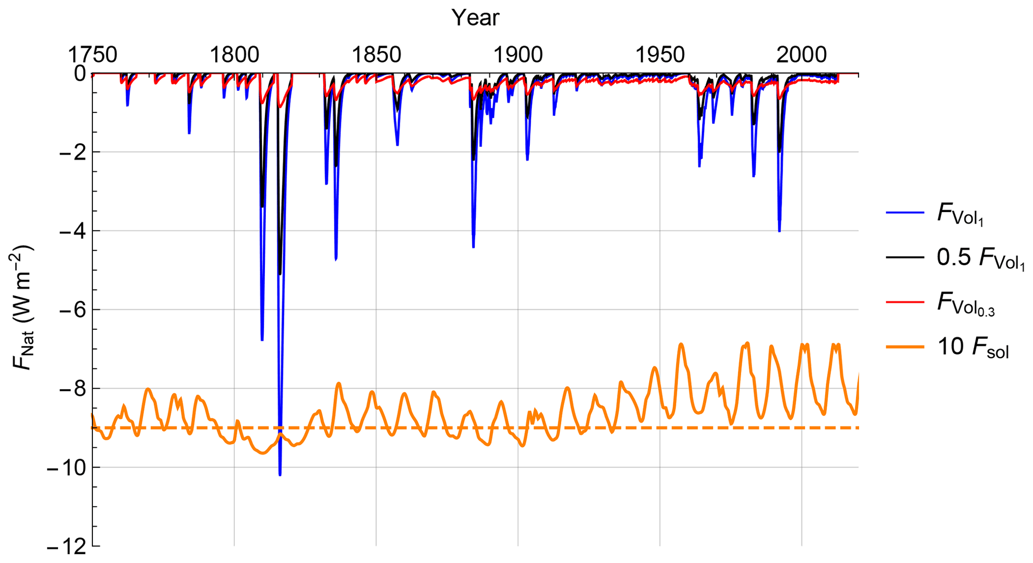
Figure 2Volcanic forcing (blue) is shown alongside two transformed versions: linearly damped by a constant 0.5 coefficient (black) and non-linearly transformed using Eq. (11) with ν=0.3 (red). The solar forcing FSol (orange) has been shifted down by −9 and amplified by a factor of 10 for clarity. The figure has been adapted from Hébert et al. (2021).
2.2.5 Volcanic forcing
The volcanic forcing series, FVol, used in this study was generated from the volcanic optical depths, τV. Over the 1850 to 2012 period, we use the approximate relation: W m−2τV, obtained from the Goddard Institute for Space Science (GISS) website (Sato et al., 1993). We follow Hébert et al. (2021), extending the series to 1765 using the optical depth reconstruction of Crowley et al. (2008) and setting volcanic forcing to zero for the future.
It is well established that volcanic forcing must be scaled down by 40 %–50 % in order to produce a comparable effect on surface temperature, and thus most EBMs linearly scale volcanic forcing (Tomassini et al., 2007; Ring et al., 2012; Lewis and Curry, 2015; Gregory and Andrews, 2016). However, the amplitude of the volcanic forcing is not the only issue; volcanic forcings are highly intermittent (spiky). The intermittency can be quantified in a multifractal framework (Lovejoy and Schertzer, 2013; Lovejoy and Varotsos, 2016) by the intermittency parameter C1 which corresponds to the fractal codimension (i.e. 1-D, where D is the fractal dimension of the part of series that gives the dominant contribution to the mean of the series) characterizing the sparseness of volcanic “spikes” of mean amplitude. There is also a multifractal index αMF that describes how quickly the intermittency changes as we move away from the mean. Since linear response models do not alter the intermittency, the volcanic series must first be non-linearly transformed before being introduced into a linear response framework. With the effective volcanic forcing , the volcanic intermittency correction exponent ν and the mean of the whole volcanic series 〈FVol〉, we follow Hébert et al. (2021) using a non-linear relation to change the intermittency so that the transformed signal can be linearly related to the temperature:
The normalization is such that the mean is unchanged: ; the average volcanic forcing is conserved – this was done for simplicity and if needed future work could include another scaling parameter (this is slightly different than the normalization used in Hébert et al., 2021). The volcanic intermittency correction exponent, ν, required to reduce the intermittency parameter of the volcanic forcing, , to equal the corresponding parameter of the temperature response, , can be calculated theoretically using:
where αMF is the multifractality index of the volcanic forcing and C1 is the codimension of the mean (see Chapter 4, Lovejoy and Schertzer, 2013).
The volcanic response appears to be non-linear as the intermittency (“spikiness”, sparseness of the spikes) parameter C1 changes from about for the input volcanic forcing to for the temperature response: the latter is therefore much less intermittent than the former, although it is possible that the estimated C1 changes slightly due to finite size effects and internal variability. Assuming αMF≈1.5 (Lovejoy and Schertzer, 2013; Lovejoy and Varotsos, 2016), we find an approximate but plausible theoretical estimate of the volcanic intermittency correction exponent ν≈0.3.
2.2.6 Internal stochastic forcing
We consider the standard assumption about internal variability that it is forced by a Gaussian “delta-correlated” white noise (Hasselmann, 1976):
where f(t) is the noise at infinite resolution, γ(t) is a “unit” white noise and σ is its amplitude. When averaged to resolution τr=1 month, the average forcing has amplitude . In comparison, the internal variability of the mean observational temperature series is equal to the observed series with the forced temperature response removed. We take the global annually averaged monthly temperature anomaly to be ∘C, where τr is the resolution (taken to be monthly in this case).
Using Lovejoy et al. (2021) and Lovejoy (2022) and , we can relate and :
where Kh is a standard normalization constant, τ is the relaxation time, and s is the climate sensitivity parameter; Eq. (14) is an approximation to the FEBE response to white noise forcing valid at short timescales τr≪τ. If we introduce a white noise forcing, with the standard deviation calculated using Eq. (14), the FEBE response will correspond to an internal variability term with realistic amplitude and autocorrelation structure.
Working in a linear framework, we write the forcing series, ℱ, as the sum of the deterministic forcings, F, (GHG, aerosol, solar and volcanic) and the white noise forcing:
where is a unit of white noise at resolution τr and “〈 〉” is the mean ensemble (statistical) average.
2.2.7 Surface air temperature data and CMIP5/6 simulations
We used five historical records of surface air temperature for our analysis each spanning the period 1880–2020, with median monthly temperature anomalies in relation to the reference period of 1880–1910: Hadley Centre/Climatic Research Unit Temperature version 4 (HadCrut4, Morice et al., 2012), the Cowtan and Way reconstruction version 2.0 (C&W, Cowtan and Way, 2014a, b; Cowtan et al., 2015), GISS Surface Temperature Analysis (GISTEMP, Lenssen et al., 2019), NOAA Merged Land Ocean Global Surface Temperature Analysis Dataset (NOAAGlobalTemp, Zhang et al., 2019; Huang et al., 2020) and Berkeley Earth Surface Temperature (BEST, Rohde and Hausfather, 2020).
The HadCRUT4 dataset is a combination of the sea-surface temperature records: HadSST3 was compiled by the Hadley Centre of the UK Met Office along with land surface station records: CRUTEM4 from the Climate Research Unit in East Anglia; the Cowtan and Way dataset uses HadCRUT4 as raw data but interpolates missing data that would lead to bias especially at high latitudes by infilling missing data using an optimal interpolation algorithm (kriging); we use the dataset with land air temperature anomalies interpolated over sea ice. The GISTEMP dataset combines the Global Historical Climate Network version 3 (GHCNv3) land surface air temperature records with the Extended Reconstructed Sea Surface Temperature version 4 (ERSST) along with the temperature dataset from the Scientific Community on Antarctic Research (SCAR) and is compiled by the Goddard Institute for Space Studies; the NOAA National Climate Data Center uses GHCNv3 and ERSST but applies different quality controls and bias adjustments. The final dataset, BEST, makes use of its own land surface air temperature product along with a modified version of HadSST.
The selected CMIP5 models have monthly historical simulation outputs available over the 1860 to 2005 period along with outputs of scenario runs from 2005 to 2100 for RCP2.6, RCP4.5 and RCP8.5, summarized in Table A1. The CMIP6 model outputs have monthly historical simulations from 1860 to 2014 and future projections based on the SSP scenarios 1-26, 2-45 and 5-85 (Forster et al., 2020) and the climate sensitivity of models are summarized in Table A2 (Flynn and Mauritsen, 2020).
2.3 Bayesian parameter estimation
In this section, we establish a procedure to estimate the probability distribution associated with the climate sensitivity: s, model parameters: τ, h and forcing parameters: α, ν. To estimate them, we relate the forcing to surface air temperature data using the FEBE with a multi-parameter Bayesian technique. To apply Bayesian inference, we require temperature observations, a statistical model that relates forcing data to temperature and prior information about the model parameters (priors). Bayesian inference is chosen due to its ability to better constrain model parameters by using information from different sources including data and models.
Through this framework, each parameter combination (h, τ for G0,h and α, ν for F as well as s) produces a time-dependent forced response which is associated with a likelihood that depends on how well the corresponding model output matches the observational temperature records over the historic period. To see how this works, recall that the FEBE describes the temperature response to the sum of the external deterministic forcing F(t) and an amplitude σ internal stochastic forcing σγ(t):
where Text, Tint indicates the responses, and * indicates convolution (Eq. 3). Any given set of parameters defines a forced temperature response Text(t), and when removed from the observation temperature series, they define a series of residuals:
The residuals are thus equal to the internal temperature variability, i.e. the response to the internal forcing σγ(t). Here, we make the usual assumption that γ(t) is a Gaussian white noise so that Tres(t)=Tint(t) is a fractional relaxation noise process (fRn, Lovejoy, 2022). However, for scales shorter than the relaxation time τ (of the order of years), the fRn process is very close to a fGn process (due to the approximation , Eq. 8). Thus, rather than making an ad hoc assumption about the statistics of the residuals, in our approach the statistics are given by the model itself (a key improvement from Hébert et al., 2021). The fGn approximation takes into account the strong power-law correlations induced by the fractional derivative term in the FEBE and it is generally valid except at the low frequencies that only weakly influence the likelihood function. An fGn model for the residuals is more realistic with respect to the autocorrelation function of temperature data (Lovejoy et al., 2015) and thus produces more conservative credible intervals in comparison to other exponential decorrelation models such as an AR(1) since the latter underestimate the decorrelation time and thus overestimate the effective sample size.
To calibrate the FEBE, we take the time-dependent forced response calculated for each parameter combination and remove it from the temperature series to obtain a series of residuals which represent an estimator of the historical internal variability. The likelihood function (ℒ) corresponds to the probability (“Pr”) of observing the series T(t) conditioned on the parameters: s, h, τ, α, ν (right-hand side), assuming the residuals are a fGn process with parameter h, and zero mean:
Using Bayes' rule, we can obtain the posterior probability density function (PDF) for our parameters using the likelihood function (an a priori probability) and the prior distribution for the parameters, :
We use the following Mathematica 12.2 (Wolfram Research, Inc., 2020) functions: LogLikelihood[proc, data], FractionalGaussianNoiseProcess[μ, σ′, h′] and EstimatedProcess[data, proc] to calculate the maximum likelihood of those residuals to be a fGn corresponding to our error model. Note that the Hurst exponent h′ used within Mathematica 12.2 describes the scaling behaviour of the associated fractional Brownian motion obtained by integrating the fGn so that . The notation corresponds to the associated exponent in Lovejoy et al. (2015), which directly describes the scaling associated with the fluctuations of the fGn itself.
The priors chosen here are intended to reflect knowledge about the historical climate system. Following Del Rio Amador and Lovejoy (2019), who estimated h from the statistics of the response of the internal forcing, the prior distribution for the scaling parameter is taken to be a normal distribution centred around 0.4 with a standard deviation of 0.1 (twice that of Del Rio Amador and Lovejoy, 2019, i.e. N(0.4, 0.1)). For the relaxation time τ, we use the normal distribution of the fast time response of the “two-box” exponential model that corresponds to h=1, found by Geoffroy et al. (2013) for a suite of 12 CMIP5 GCMs: N(4, 2 yr), with the standard deviation doubled of the original work so as to be a weakly informative prior. When considering the aerosol scaling parameter, α, we take the prior distribution to be a normal distribution, N(1.00, 0.55), which has a 90 % CI and mean coherent with the IPCC AR5 best range for the modern value of aerosol forcing, W m−2, in the series we used. For the remaining two parameters, s and ν, we assume non-informative uniform priors over the range of parameters; and . All prior distributions are independent.
Using Bayes, Eq. (20), we then fit a multivariate Gaussian distribution to our five-dimensional parameter space, posterior distribution , which will be used to draw sets of parameters to generate future forced temperature projections. The multivariate Gaussian approximation is built by using the means and variances of all parameters through integrating the joint probability to obtain five marginal probabilities and calculating the covariance between all pairwise parameters using their “joint” marginal distributions as to take into account potentially large correlations between parameters. The five-dimensional posterior parameter space, (s, h, τ, α, ν) is thus defined by a multivariate normal distribution:
where , the vector of the means is μ and the 5×5 covariance matrix Σ.
Using Bayes' theorem as described above, we derive PDFs for the model and forcing parameters of the FEBE from the mean likelihood functions of the five observational datasets. The different observational datasets are treated as dependent due to the use of overlapping raw data, with the differences between series coming partly from the different processing of the raw data by different teams. This corresponds to putting the datasets into a Bayesian framework where each has equal a priori probability: HadCRUTv4, C&W, GISTEMP, NOAAGlobalTemp and BEST (n=5).
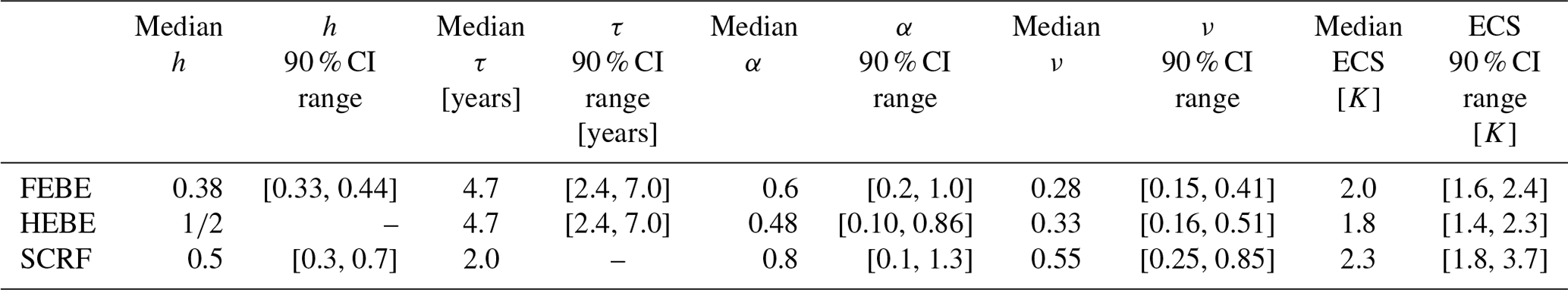
Following IPCC methodologies, we report the “very likely” credible interval at the 90 % credible level throughout this work along with median estimates for the all ensemble spreads. The complete suite of model and forcing parameters and climate sensitivities are summarized in Tables 1 and 2. In addition, we include a comparison of the same parameters for the half-order EBE (HEBE) () that is a consequence of the classical continuum heat equation (Lovejoy, 2021a, b), as well as with the precursor scaling climate response function (SCRF) model (Hébert et al., 2021) which differs primarily in the treatment of high frequencies in Table 3. The FEBE value of h is slightly less than 0.5 and corresponds to energy balance with the fractional heat equation.
Table 1Model and forcing parameter medians for FEBE calibrated over the historical period (1880–2020) using and , along with their corresponding 90 % credible intervals.
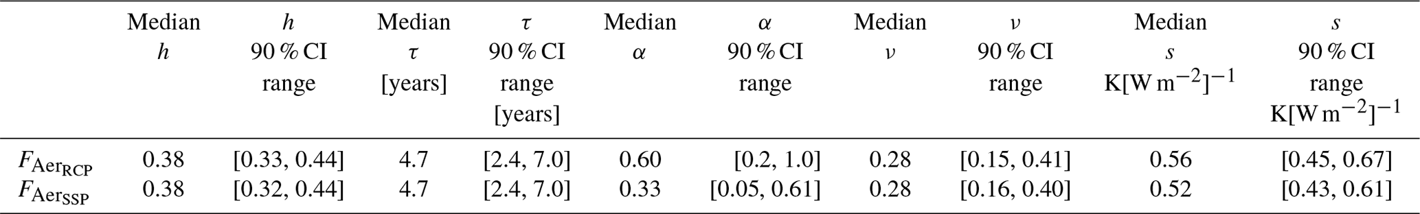
Table 2The calculated ECS and TCR medians using both parameters corresponding to and , along with their corresponding 90 % credible intervals.
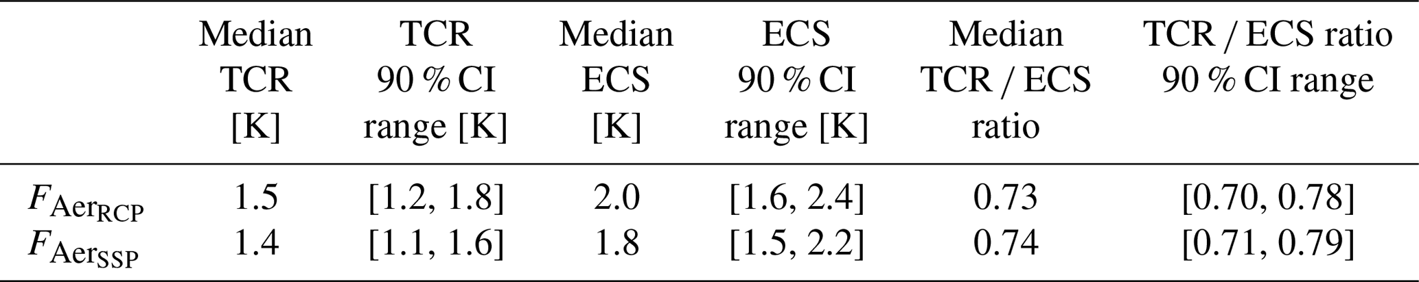
Table 3Model and forcing parameter medians using for FEBE, the classical continuum mechanics HEBE () and the SCRF model (Hébert et al., 2021) calibrated over the historical period, along with their corresponding 90 % credible intervals.
3.1 The model: Green's function parameters: h, τ
3.1.1 The scaling exponent h
The model is characterized by h and τ, where the exponent h of the FEBE is the most fundamental. For h, we found a 90 % CI of [0.33, 0.44] shown in Fig. 3a, with a median value of 0.38 when using , and while using we found a similar median of 0.38 with 90 % CI of [0.32, 0.44]. We can already note that it is close to the HEBE value and other empirical estimates for power-law impulse Green's functions () with (Lovejoy et al., 2017; Hébert et al., 2021). The NOAA dataset differs the most from all others; the exact cause of the difference is not clear, although it arises from the Merged Land–Ocean Surface Temperature Analysis (MLOST) dataset's use of a complex algorithm with low-frequency tuning (Smith et al., 2008). This low-frequency tuning along with the spatiotemporal smoothing applied in the MLOST dataset is likely the cause of a slightly higher h (i.e. a smoother temperature series).

Figure 3For each observational dataset and their average, PDFs are shown for the model parameters: the scaling parameter h (a) and the transition time τ (b). Shown are the PDFs for parameter estimation based on both (solid) and (dashed). The average PDF of the five observation datasets using is shown as the main result with shading, with darker 5 % tails.
3.1.2 The relaxation time τ
The second model parameter is the relaxation time τ that characterizes the approach to equilibrium. From the point of view of parameter estimation, τ is a difficult parameter to determine since it is inversely correlated with s: a large τ can be somewhat compensated by a smaller s, and vice versa. As shown in Fig. 3b, we obtained the a posteriori median value of 4.7 years and 90 % CI of [2.4, 7.0] years when using and nearly identical results using .
Presented in Fig. 4a is the step-response Green's function, , of the FEBE with the parameters h and τ along with its 90 % CI, shown alongside the IPCC two-box-model Green's function (Held et al., 2010; Geoffroy et al., 2013; IPCC, 2013). Considering G1 (blue), at scales below a few years where the box models or the Hébert et al. (2021) truncated scaling model are smooth, the FEBE has a singular response. This enables it to reproduce the statistics of the internal variability as well as to be more sensitive to volcanic forcings. Even at scales of up to 25 years, the G1 (blue) responds much faster than the IPCC (black), yet the approach to the asymptotic value of 1 corresponding to energy balance is substantially slower. This can also be seen in the ramp-response Green's functions (Fig. 4b), G2, the integral of G1. For comparison, each was normalized by the value at 70 years – the standard ramp time for TCR (Collins et al., 2013). At multi-year resolution (ignoring the high-frequency variability), over the scale of the Anthropocene, there is little difference between the FEBE and IPCC, with FEBE having a more gradual response. This contributes to the somewhat cooler FEBE centennial-scale projections when compared with those from the two-box model.
3.2 Characterizing the forcing
3.2.1 Aerosol linear scaling factor α
The aerosol linear scaling factor α that effectively recalibrates the aerosol forcing (Fig. 5a, solid line) was found to have a median value of 0.6 with a 90 % CI of [0.2, 1.0] for the CMIP5 series. However, when using the CMIP6 sulfate-emissions-based aerosol forcing series, , we find support for a weaker and better-constrained aerosol forcing, recalibration α with a median of 0.33 and 90 % CI of [0.05, 0.61] (Fig. 5a, dashed line). In both cases, an aerosol recalibration factor of 1 corresponds to the modern (2005) aerosol forcing value of about −1.0 W m−2, but we find in both cases that α<1. The result from two independent aerosol forcing series again shows that the forcing associated with aerosols is still widely uncertain and overpowered, supporting post-AR5 studies that found aerosol forcings simulated by GCMs were unrealistic (Zhou and Penner, 2017; Sato et al., 2018; Bellouin et al., 2020) and that aerosol forcing was weaker when climate feedbacks were allowed (Nazarenko et al., 2017).
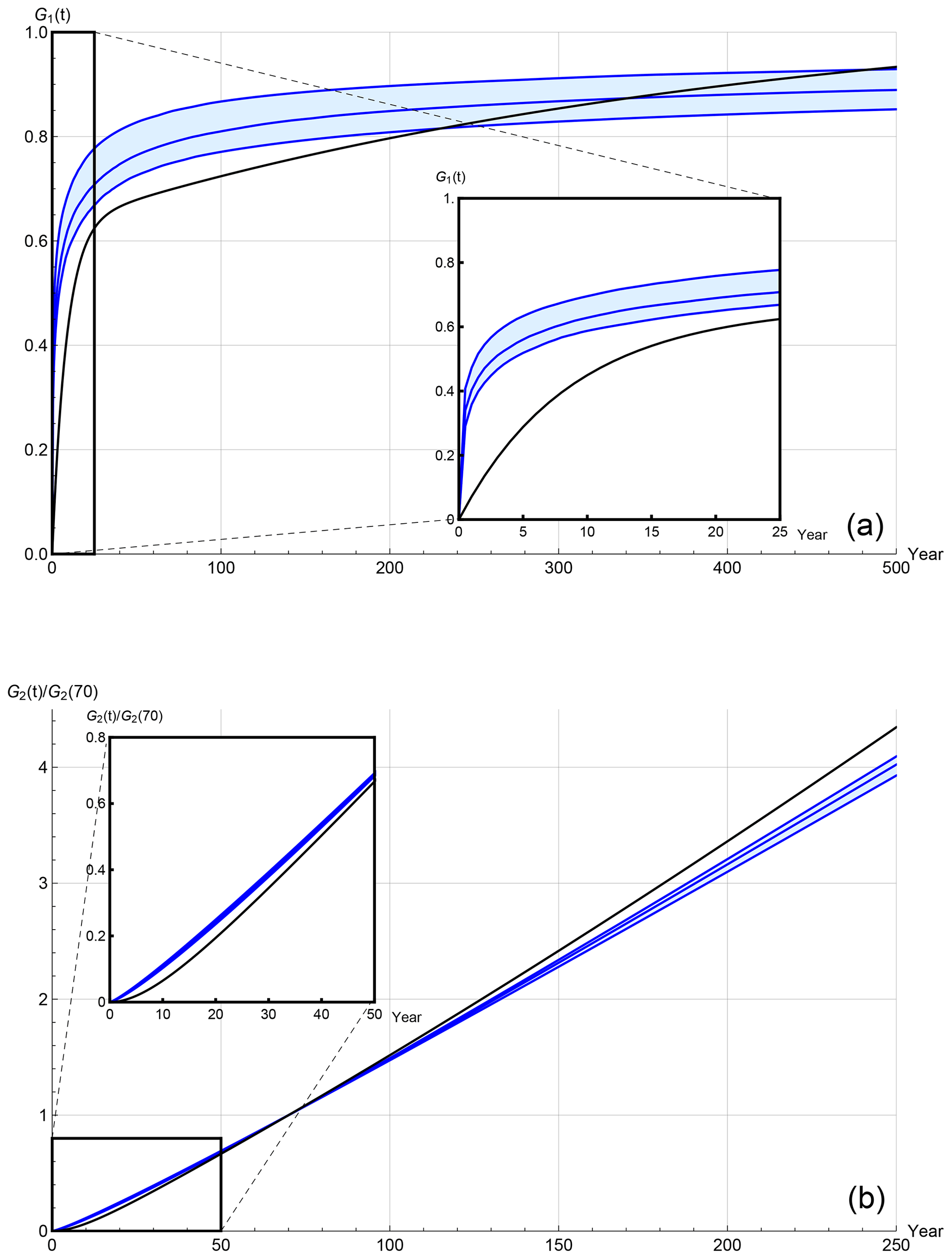
Figure 4(a) The median and 90 % CI of the FEBE step-response Green's function, , compared to the IPCC two-box-model Green's function (black). (b) The median and 90 % CI of the FEBE normalized ramp-response Green's function, , compared to the IPCC two-box-model Green's function (black).
3.2.2 Volcanic intermittency correction exponent ν
The volcanic intermittency correction exponent ν was found to have a posterior median value of 0.28 with 90 % CI of [0.15, 0.41] when using and similar median value 0.28 with 90 % CI of [0.16, 0.40] when using (recall ν=0 implies a constant mean forcing and the original series is recovered with ν=1). Both contain the theoretically calculated ν within their 90 % CI (ν=0.32). This result confirms that volcanic forcing is generally overpowered since ν=1 has nearly null probability as seen in Fig. 5b. Thus, the original volcanic series described without the intermittency correction does not reproduce well, within the FEBE model presented, the cooling events observed in instrumental records following eruptions: volcanic cooling would be overestimated. As noted in the case for the exponent, h, the NOAA dataset noticeably differs from the others; the spatiotemporal smoothing applied in the MLOST dataset is likely the cause of a lower ν (i.e. a smoother volcanic forcing).
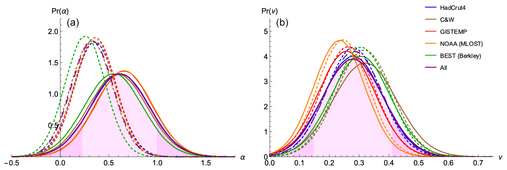
Figure 5For each observational dataset and their average, PDFs are shown for the forcing parameters: the aerosol scaling factor α (a) and the volcanic intermittency correction exponent ν (b). Again, shown are the PDFs for parameter estimation based on both (solid) and (dashed). The average PDF of the five observation datasets using is shown as the main result with shading, with darker 5 % tails.
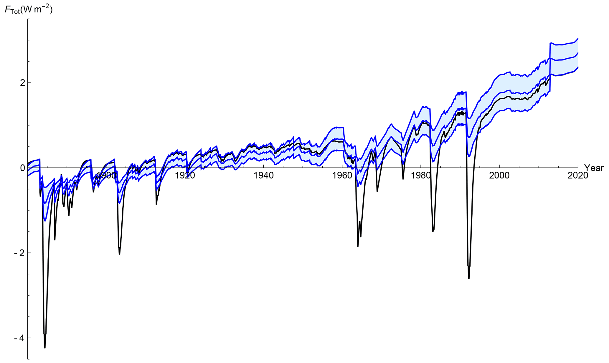
Figure 6The total historical (1880–2020) forcing series prescribed by the IPCC using, (black) compared to the adjusted forcing, (blue), which takes into account aerosol and volcanic corrections, shown with 90 % CI.
In Fig. 6, we compare the total forcing series, FTot(t) (black), IPCC AR5, Eq. (16), where , with the adjusted forcing series, (blue). During the historical period, the intermittency and strength of the strong volcanic events are greatly reduced, and in the recent past the median-adjusted forcing series is higher than the unadjusted forcing due to the reduced aerosol forcing strength. This adjusted forcing series consequently contributes to a lower climate sensitivity, presented in the following section, due to the historic negative forcings of volcanoes and aerosols being adjusted to closer match historical observations, eliminating the need for a high climate sensitivity to compensate.
3.3 Climate sensitivity
3.3.1 Climate sensitivity parameter, s
The climate sensitivity parameter s refers to the equilibrium change in the annual global mean surface temperature (GMST) following a unit change in radiative forcing. Its inverse is the climate feedback parameter, the increase in radiation to space per unit of global warming. We find s to have a median value of 0.56 K(W m with 90 % CI [0.45, 0.67] K(W m using , and when using we find median 0.52 K (W m with 90 % CI [0.43, 0.61] K(W m (Fig. 7), both on the lower end of the CMIP5 MME climate sensitivity parameter of median 1 K(W m and 90 % CI [0.5, 1.5] K(W m but within the 90 % CI. However, both estimates are below the CMIP6 MME 90 % CI [0.63, 1.50] K(W m, with a median of 0.92 K(W m, which has been criticized as being too high (Zelinka et al., 2020; Tokarska et al., 2020; Flynn and Mauritsen, 2020).

Figure 7For each observational dataset and their average, PDFs are shown for the climate sensitivity parameter s (the ECS, here in units of K (W m−2)−1), (solid) and (dashed).
3.3.2 Equilibrium climate sensitivity
Two standard types of climate sensitivity used for inter-model comparisons: ECS and TCR – our results are summarized in Table 2.
If atmospheric CO2 was increased to double pre-industrial concentrations and then held there, the planet would only slowly reach a new equilibrium. This delay is largely because the world's oceans take a long time to heat up in response to the enhanced greenhouse effect. The ECS is the amount of warming achieved when the entire climate system reaches “equilibrium” or the steady-state temperature response to a doubling of CO2. By the definition of the temperature response to external forcings in Eq. (7), the climate sensitivity parameter is the equilibrium climate sensitivity. The two are equivalent to within a constant factor: the number of W m−2 per CO2 doubling, the standard value being 3.71 W m−2/(CO2 doubling) (IPCC, 2013).
The PDF for ECS shown in Fig. 8a, for both aerosols series, was found to have a 90 % CI of [1.6, 2.4] K and a median value of 2.0 K when using , and median of 1.8 K and 90 % CI [1.5, 2.2] using (see Table 2). These results are lower than those found in the CMIP5 MME which had a best value of 3.2 K, but our 90 % CI bounds are more narrow, laying within the CMIP5 MME range of [1.9, 4.5] K. Although when we consider the expanded ECS 90 % CI of [1.5, 4.5] K considered in IPCC (2013), which takes into account both the CMIP5 MME and historical estimates, we see that the FEBE estimates are wholly within this range and much less uncertain. For the CMIP6 MME which has a 90 % CI of [2.0, 5.5] K and mean estimate 3.7 K, our best estimate using the corresponding is slightly below the lower credible interval due to the upward shift of ECS estimates seen in CMIP6 models (Zelinka et al., 2020) but again has a more narrow CI.
3.3.3 Transient climate response
Conventionally, TCR quantifies the temperature change that would occur if CO2 levels increase by 1 % (compounded) per year until they double (≈70 years). Since the CO2 forcing is logarithmically dependent on CO2 concentration, the TCR is then simply the global temperature increase that has occurred at the point in time that a linearly increasing forcing reaches double pre-industrial levels.
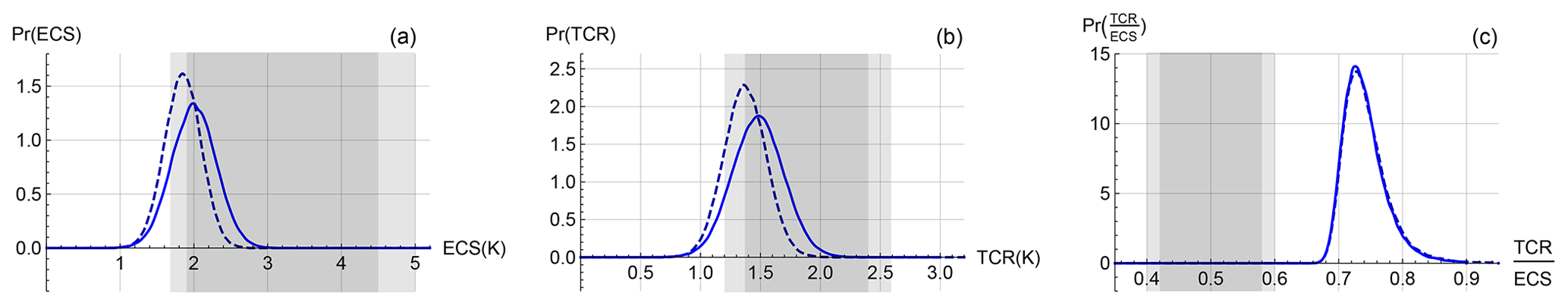
Figure 8The PDFs for ECS (a), TCR (b) and the TCR-to-ECS ratio (c) are derived using (solid) and (dashed). The associated 90 % CI (bars under the axis), the CMIP5 MME 90 % CI (dark grey shading) and the CMIP6 MME 90 % CI (light grey shading) are shown.
The derived PDFs for TCR are shown in Fig. 8b and summarized in Table 2. Our TCR was found to have a 90 % CI of [1.2, 1.8] K with a median of 1.5 K when using , while when using we find a median 1.4 K and 90 % CI of [1.1, 1.6] K. Both estimates are lower and more constrained but within the 90 % CI given by the CMIP5 MME: a 90 % CI of [1.2, 2.4] K and a best value of 1.8 K, and by the CMIP6 MME: 90 % CI of [1.2, 2.8] K with best value of 2.0 K.
The ECS and TCR estimates using the SSP scenarios with the FEBE are lower than those using RCPs due to the overly strong aerosols over the historical period in the SSPs which require a lower aerosol linear factor along with lower ECS to best match the historical temperature record. The difference between the shape of the RCP and SSP aerosol forcing can also account for this.
The TCR-to-ECS ratio is a non-dimensional measure of the fraction of committed warming already realized after a steady increase in radiative forcing; in this case, with a doubling of CO2, this quantity is generally referred to as realized warming fraction (RWF) (Stouffer, 2004; Solomon et al., 2009; Millar et al., 2015); it is a non-dimensional memory parameter. A model with a low RWF will indicate that global warming may continue for centuries after emissions have stopped. We present the TCR-to-ECS ratio in Fig. 8c, with a 90 % CI [0.70, 0.78] and median 0.73 using FRCP parameters. Similar results are found using FSSP parameters, a median of 0.72 and 90 % CI [0.71, 0.79]. From Fig. 8 and Table 2, we see that the TCR-to-ECS ratio is higher than both generations of MME 90 % CI, a consequence of lower ECS and TCR values, and similar uncertainty.
In the next section, we show that with a lower and more constrained climate sensitivity parameter (Figs. 7 and 8), the adjusted forcings (Fig. 6) and long memory process of the FEBE produce future projections that tend to be cooler than the CMIP5/6 projections, yet remain within their 90 % CI.
4.1 Uncertainties
With the above collection of model and forcing parameter probability distributions, the FEBE was used to reconstruct the temperature over the historical period, as well as make projections of the forced temperature response for the coming century using forcings prescribed by the RCP and SSP scenarios.
The CI provided for the MME corresponds to the spread between the different GCMs, “structural uncertainty”, while for the FEBE it is parametric uncertainty (Bretherton, 2012). In both cases, the projections are deterministic but with uncertainty limits due to their respective model uncertainties. Both yield an estimate of the forced response but with qualitatively different uncertainty bounds.
For the FEBE, the spread of the forced projections is purely from the uncertainty in the parameters: the contribution to uncertainty from internal variability has been averaged out (it is effectively the average over an infinite ensemble of realizations of internal variability). In order to make projections, we therefore draw samples of parameters from the (correlated) multidimensional parameter space (approximated by the multivariate normal distribution in Eq. 21), by using a Monte Carlo method. Once a random set of parameters has been chosen, realizations of the forced temperature response are generated using Eq. (3) and a numerical convolution. It should be noted this Monte Carlo sampling is simply a convenient numerical technique for performing high-dimensional probability space integrals; it does not imply any stochasticity in the projections which, although parametrically uncertain, are nevertheless deterministic responses to purely deterministic forcing. However, the Monte Carlo methods do introduce standard Monte Carlo numerical uncertainty, but this was made quite small by using a large number (500) of Monte Carlo realizations. Once we have our ensemble of projections, we remove the pre-industrial baseline (such that the temperature anomaly over 1880–1910 is zero) and calculate the desired credible intervals of the forced response. We consider the historical period coinciding with the range of observation temperature records (1880–2020) and make all comparisons to this period, acknowledging that the CMIP5 GCM historical reconstruction ended in 2005 and for the CMIP6 GCMs in 2014.
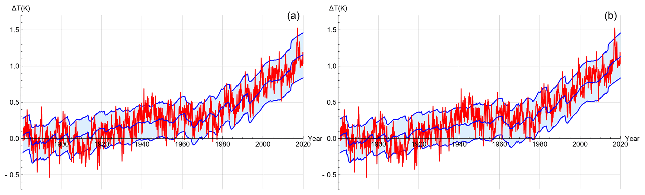
Figure 9(a) The historical reconstruction (forced temperature response and internal variability) of the FEBE, with parameters calibrated using (blue) alongside mean of five observational temperature series (red) at monthly resolution; 90 % CIs (due to parametric uncertainty and internal variability) are indicated (shaded). (b) Same as left except using parameters and forcing.
4.2 Reliability and historical reconstructions: 1880–2020
In this section, we present the full historical reconstruction using the FEBE observation-based projections with those from the GCMs in the CMIP5/6 MME. In order to make a proper comparison with data, we must include both the forced deterministic temperature response, with its purely parametric uncertainty, as well as the internal variability of the mean observational temperature series, estimated to be ∘C (monthly resolution). The two uncertainties were combined assuming the statistical independence of the internal forcing and the parametric uncertainty: the errors therefore add in quadrature.
An important characteristic of probabilistic forecasts is their reliability that quantifies the difference between the forecast and actual probability distributions. Consider for example, a set of predictions derived from ensemble forecasts. In some realizations, it is predicted that the chance of above-average seasonal-mean temperature for the coming season will be 70 %. If the probabilistic forecast system is reliable, then one can expect that in 70 % of these predictions the actual seasonal-mean temperature will be above average (Annan and Hargreaves, 2010; Weisheimer and Palmer, 2014). In Fig. 9, we can verify the reliability of the FEBE. We see that as expected, the temperature observations fall closely within the 90 % CI of the FEBE historical reconstruction (i.e. the ensemble average of the response to both internal and external forcing). More precisely, at the monthly resolution in Fig. 9, the historical mean temperature (red) is within the 90 % CI of the FEBE-forced response (with internal variability added) 89.9 % of the months using the RCP scenario (Fig. 9a) or 90.2 % of the months using the SSP scenario (Fig. 9b). The accuracy of this uncertainty verifies both the underlying model and Bayesian parameter estimation method.
This is expected for a reliable model and is an analogous validation of probabilistic aspects of the projection as unlike weather forecasts where we have many past test cases; climate change projections cannot be calibrated in the same manner (Stainforth et al., 2007; Tebaldi and Knutti, 2007; Knutti et al., 2010). Note that in both reconstructions, it is possible that the end of the second World War (1945) temperature spike which lies outside of the FEBE 90 % CI may be explained due to biases associated with bucket and engine room intake measurements (Chan and Huybers, 2021).
4.3 The amplitude of the internal forcing
The small-scale limit of the validity of the FEBE is not known, although it is likely to be ∼1 month (roughly the weather–macroweather transition timescale). Justification comes from the success of the high-frequency FEBE limit that successfully forecasts monthly and seasonal temperatures (Del Rio Amador and Lovejoy, 2019, 2021a; Del Rio Amador and Lovejoy, 2021b). As discussed earlier (Eq. 14), the FEBE predicts the (stochastic) response to the internal forcing. The standard deviation of f(t) is the amplitude of the internal forcing assumed to be Gaussian white noise, which can be estimated using Eqs. (14) and (15), and ∘C. Using our FRCP (and FSSP) parameter estimates, we find a mean estimate of the forcing standard deviation, σf, to be 3.2 W m−2 (3.3 W m−2) and 90 % CI of [2,1, 4.2] W m−2 ([2.3, 4.3] W m−2) (at a monthly resolution: τr=1 month). If we introduce a white noise forcing with amplitude, the FEBE recreates the amplitude of the internal temperature variability response and its change as a function of timescale/resolution.
This estimate of the internal variability forcing can be compared with that of Harries and Belotti (2010), who examine the net energy flux balance at the top of atmosphere (TOA) measured using observations from polar-orbiting spacecraft (at monthly scale). The early observations, using the Nimbus experiments, show an internal variability of the 4.1±4.0 W m−2, while more modern measurements (CERES) in the 2000s show variability of between ±2 and ±4 W m−2. Thus, our estimate of the internal forcing variability is within estimates of the TOA net energy flux balance.
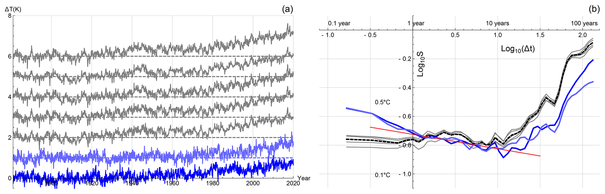
Figure 10(a) The historical reconstruction (forced and internal temperature response) of the FEBE, with parameters calibrated using (blue) and (light blue) alongside the five observational temperature series (grey – shifted up) at monthly resolution. (b) The root mean square Haar fluctuation structure function S(Δt)=〈ΔT(Δt)2〉½ for FEBE reconstruction using (blue) and (light blue), and the five globally averaged monthly resolution temperature time series (grey; mean is shown in dashed black). The reference (red) line has the slope of the approximate median estimate of the scaling exponent h≈0.4 (). The stochastic (internal variability) is not expected to be identical; only its statistical character (correlations) and amplitude are expected to be the same as the data.
4.4 Statistical evaluation of the FEBE
As with GCMs, the FEBE predicts the forced deterministic response as well as the statistical properties of the internally driven stochastic part. We can therefore evaluate the accuracy of the stochastic part by comparing the FEBE temperature statistics with those from observational time series. It was already shown in Lovejoy et al. (2021) that using a simple “ramp” model that included the deterministic external and stochastic internal variabilities the FEBE roughly predicts both high- and low-frequency scaling regimes. In Fig. 10a, we show one realization of the full FEBE, including the deterministic and stochastic forcings, with median parameters calibrated earlier using (blue) and (light blue); the five observation temperature series are shown alongside (grey – shifted up). We compare the model statistics with the five globally averaged temperature series using their root mean square Haar fluctuations, shown in Fig. 10b. The Haar fluctuation for a series T(t), ΔT(Δt) is the difference between the average of the first and second halves of the interval Δt. This is a convenient way to characterize variability as a function of timescale in real space, valid for increasing or decreasing average fluctuations. By applying global-scale Haar fluctuation analyses, Del Rio Amador and Lovejoy (2019) found corresponding to .
Below Milankovitch timescales, there are three main scaling regimes observed in the atmosphere: the weather, macroweather and climate (Lovejoy, 2013). In the macroweather regime, longer than the lifetime of planetary structures (∼10 d), temperature fluctuations decrease with scale until a transition probably occurs to the climate regime where fluctuations begin to increase. In the industrial epoch, this scale is ∼20 years, while in the pre-industrial epoch this scale's transition occurs at centuries or millennia (Lovejoy, 2015b). Over the scale of 1 year to about 10 years (the macroweather regime), the FEBE and the observational temperature series have an approximate slope (indicated by the straight reference line in Fig. 10b) of h≈0.4. We see a transition in both the FEBE and observations at Δt⪆10 years: the transition to the climate regime where fluctuations begin to increase with scale. The fact that the FEBE's fluctuations at the climate regime track the observational data strongly supports the realism of the FEBE for multidecadal projections.
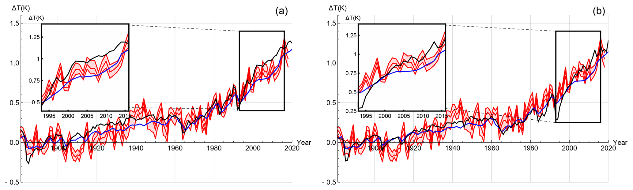
Figure 11(a) The median historical forced component of the FEBE, with parameters calibrated using (blue) and the median of the CMIP5 MME (black) alongside mean of five observational temperature series (red) with their 90 % CI indicated (shaded). (b) The median historical forced component of the FEBE, with parameters calibrated using (blue), and the median of the CMIP6 MME (black) alongside the mean of five observational temperature series (red) with the 90 % CI indicated (shaded).
4.5 Evaluating the FEBE using hindprojections including the slowdown
We have shown that the FEBE hindcasts are reliable (Sect. 4.2), that they have realistic internal forcings (Sect. 4.3) and realistic statistical variability (Sect. 4.4). Here, we evaluate their deterministic responses using hindprojections.
Unlike the comparison in Fig. 10 that included the internal variability in order to evaluate the reliability, the following figures are estimates of the ensemble averaged hindprojections, i.e. with the internal variability averaged out completely. This is not a reliability check at 1-year resolution, as shown in the prior section, so we do not expect the FEBE to be in the data range 90 % of the time. Rather, the percentage of the time that the FEBE is in the data range is a measure of hindprojection–data agreement about the deterministic forced response part. It is therefore appropriate to compare this with the MME. In Fig. 11, we compare the 90 % CI of the historical temperature observations with the median-forced response of both the FEBE using the RCP (Fig. 11a) and SSP (Fig. 11b) historical forcing compared to both the CMIP5 (Fig. 11a) and CMIP6 (Fig. 11b) MMEs. In the inset of Fig. 11, we show the slowdown (“hiatus”) period (1998–2014).
Throughout the historical period, the hindprojection of the FEBE and the median of the CMIP5/6 MME are close. Between 1915–1960, the CMIP5/6 MME is consistently warmer than the FEBE hindprojection and historical temperature records, although generally by less than 0.05 K. The slowdown in global warming during the first decade of the 21st century, termed as the slowdown (“hiatus”) (Kaufmann et al., 2011; Meehl et al., 2011; Medhaug et al., 2017), is tracked closely by the FEBE hindprojection, while the CMIP5/6 MME overshoot (by 0.1 to 0.2 K), a well-studied divergence between GCMs and observations, is shown in Fig. 11 (insets). This supports Lovejoy (2015a) and Lovejoy (2015b), which found that the slowdown (“hiatus”) could be well predicted by a stochastic fGn model (comparable with the present hindprojection) and concluded the issue to be GCM overprojection.
Table 4The 90 % CI of projected warming relative to the pre-industrial reference period (1880–1910) for the RCP scenarios analysed in this study based on the FEBE and the CMIP5 MME. Summary of Fig. 12a–c.
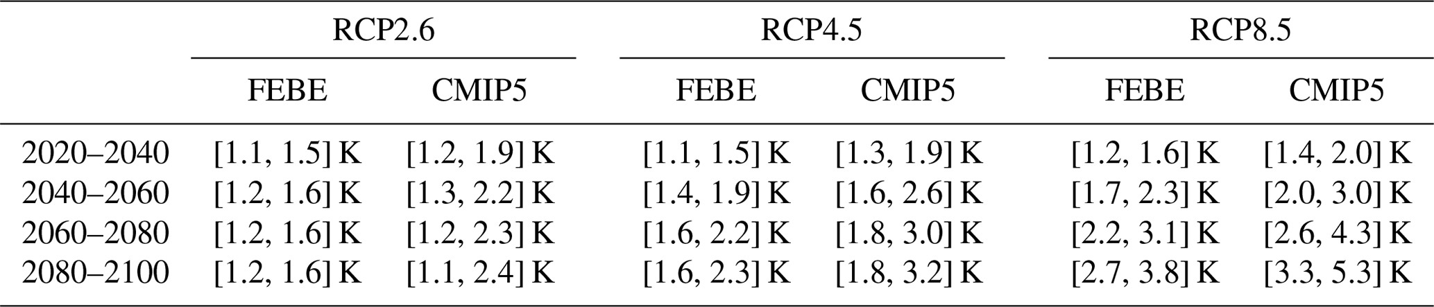
Table 5The 90 % CI of projected warming relative to the pre-industrial reference period (1880–1910) for the SSP scenarios analysed in this study based on the FEBE and the CMIP6 MME. Summary of Fig. 12d–f.
Following the monthly resolution reliability confirmation in Sect. 4.2, we can now perform a quantitative comparison between the amount of time the FEBE and CMIP5/6 MME median response is within the bounds of the observational temperature series 90 % CI performed with annual resolution data. The median FEBE hindprojection using is within the 90 % CI of the observational temperature series over the whole historic period 47 % of the years and over the slowdown is within 70 % in comparison to the CMIP5 MME median which is within the whole historic period only 39 % and over the slowdown it is 17 %. While with the median FEBE hindprojection using similar results are found, over the whole period 45 % and over the slowdown 35 %, in comparison to the CMIP6 MME median which is within the whole historic period 39 % and over the slowdown it is 30 %. In can be seen in both cases that the CMIP MME is generally warmer than the FEBE-forced component, notably over the period of the slowdown. We see that indeed the FEBE-median-forced component in both cases captures the slowdown rather accurately.
5.1 The FEBE and GCM MME comparisons
We now consider the deterministic (infinite ensemble) FEBE projections to 2100. At first, the temperature increase in each case is nearly identical; the future pathways only diverging into their respective scenarios roughly two decades after their beginning (RCPs begin in 2005; SSPs begin in 2014). Further into the future, the warming rate begins to depend more on the specified scenario, the highest being in RCP8.5/SSP5-85 (Fig. 12c and f), while they are significantly lower in RCP2.6/SSP1-26 (Fig. 12a and d; Tables 4 and 5), particularly after about 2050 when the global surface temperature response stabilizes (and declines thereafter). Of particular interest are the low-emission scenarios, RCP2.6/SSP1-26, demonstrating the potential of strong mitigation policies and speculative negative emission technologies where anthropogenic forcing starts decreasing around the mid-2040s. In this scenario, the CMIP5 MME temperature stays below 2 K throughout the 21st century, whereas the corresponding median FEBE temperature projection never exceeds 1.5 K. Comparing projected warming in 2100 for the RCP2.6/SSP1-26 scenario, the FEBE projection reaches a median warming of 1.2 K with 90 % CI of [1.1, 1.4] K, while the CMIP5 MME has a 90 % CI of [0.9, 2.4] K and median warming of 1.7 K. When considering the CMIP6 projections for SSP1-26 (Fig. 12d), the median temperature exceeds 2 K beginning near 2050, whereas the corresponding FEBE projection is consistently lower, only crossing the 1.5 K threshold briefly. In 2100, the CMIP6-projected temperature reaches 2.2 K with 90 % CI of [1.5, 2.8] K, while the FEBE projects a median temperature of 1.5 K and a narrower spread of [1.3, 1.8] K.
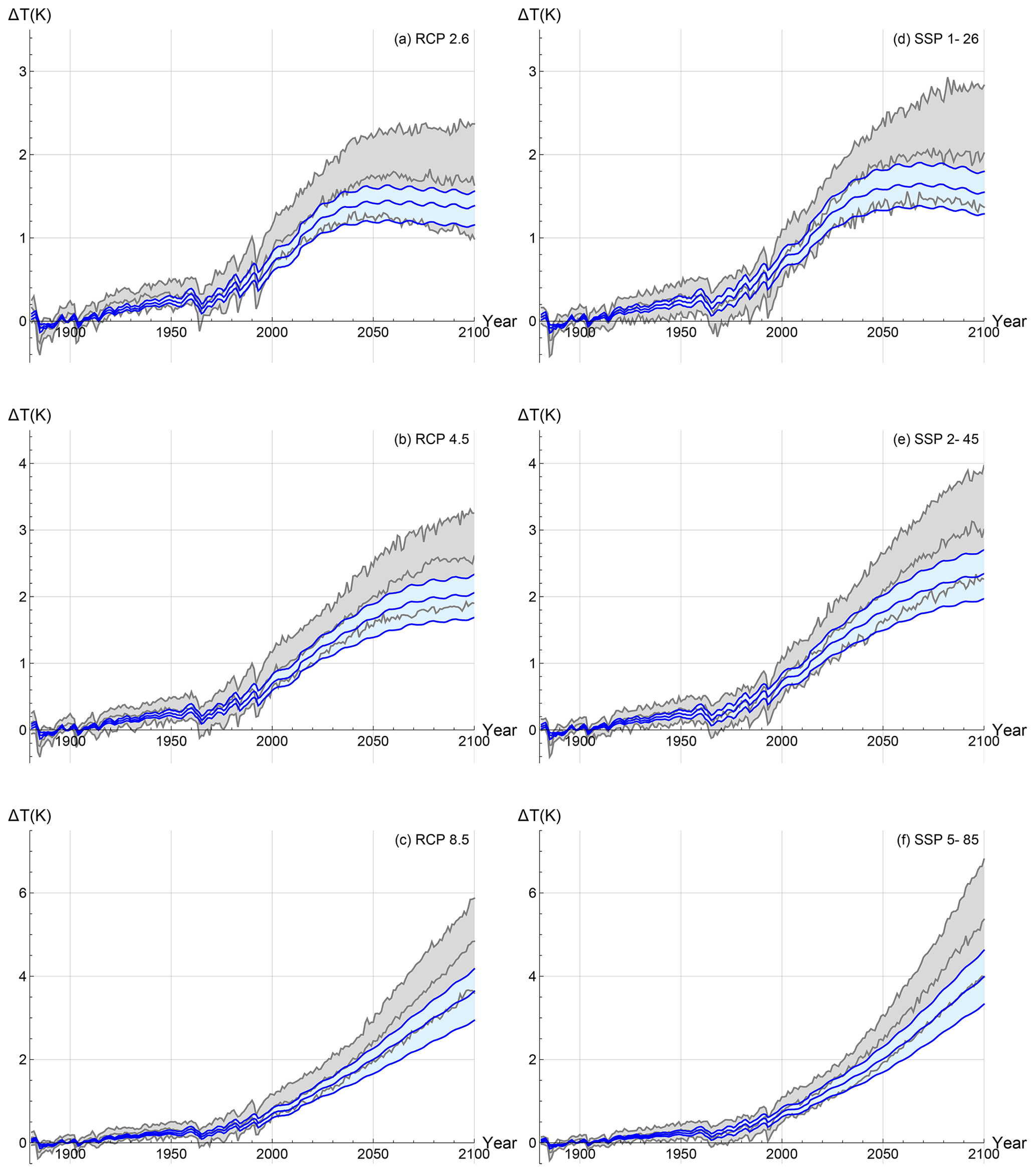
Figure 12The deterministic forced temperature response projected using the FEBE (blue), with parameters calibrated using (a–c) and (d–f) compared with the CMIP5/6 MME projection (grey); 90 % CIs from the parametric uncertainty are indicated (shaded). The projections until 2100, for RCP2.6/SSP1-26 (a, d), RCP4.5/SSP2-45 (b, e) and RCP8.5/SSP5-85 (c, f), are shown.
While the forcing of the (perhaps most realistic) middle scenario, RCP4.5/SSP2-45, stabilizes in the mid 2060s, the temperature projections continue rising throughout the 21st century for both FEBE and the CMIP5/6 MME (Fig. 12b and e). In 2100, the FEBE and CMIP5 MME project the temperature reaching 1.9 K [1.6, 2.2] K and 2.6 K [1.8, 3.2] K, respectively, shown in Fig. 12b. A key point to note is that the FEBE RCP4.5 projection remains below 2.5 K warming by 2100, while the CMIP5 MME is well beyond this threshold. Looking at the CMIP6 projections for SSP2-45 (Fig. 12e), the median temperature exceeds 2 K beginning near 2050, whereas the corresponding FEBE projection is consistently lower and begins to diverge after 2050. In 2100, the CMIP6 projected temperature reaches 3 K with 90 % CI of [2.1, 4.2] K, while the FEBE projects a median temperature of 2.3 K and a narrower spread of [1.8, 2.8] K.
The projections of both the FEBE and the CMIP5 MME for the strong emission scenario, RCP8.5, show alarming warming rates of 3.5 K with 90 % CI [2.9, 4.1] K and 4.8 K with 90 % CI [3.5, 6.0] K in 2100 shown in Fig. 12c and f. The same quickly increasing trend is seen in the CMIP6 SSP5-85 scenario, with temperatures in 2100 reaching a staggering 6.2 K with 90 % CI [4.5, 7.0] K, while the FEBE projection, although lower at 3.8 K and having a tighter bound of [3.5, 4.5] K, shows the dire consequences of no mitigation. All results shown in Fig. 12 are summarized in Tables 4 and 5.
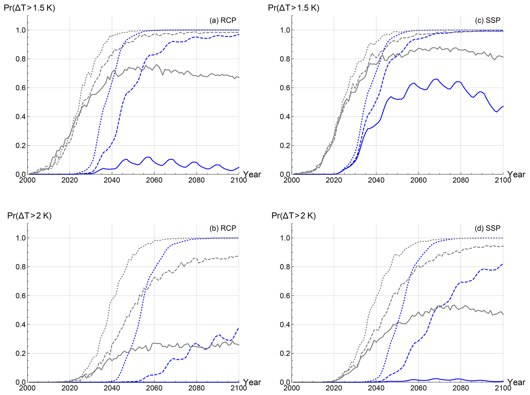
Figure 13The probability for the global mean surface temperature of exceeding a 1.5 K threshold (a, c) and a 2 K (b, c) are given as a function of years for the FEBE (blue), using (a, b) or (c, d) and for the CMIP5/6 MME (grey). The three scenarios are considered for each case: RCP2.6/SSP1-26 (solid), RCP4.5/SSP2-45 (dashed) and RCP8.5/SSP5-85 (circles).
Whereas the CMIP5 projections differ from the CMIP6 projections due to both model and forcing series changes, the FEBE projections differ only because of the changes in the forcing series. By comparing the left and right columns of Fig. 12, we can quantify the difference in projected warming caused by the changing of the forcing series and between CMIP model generations. In the year 2100, we see the FEBE is 1.4 K above pre-industrial levels in the RCP2.6 scenario, whereas in the SSP1-26 scenario it is 1.5 K above this (a difference of 0.1 K). In comparison, for the same two scenarios, the CMIP5 MME is 1.6 K and the CMIP6 MME is 2.0 K above pre-industrial levels, respectively (a difference of 0.4 K). The same can be done for the other two scenarios: for the RCP4.5/SSP2-45 scenarios, the FEBE is found to have warming in 2100 of 2.1 and 2.3 K (a difference of 0.2 K) above pre-industrial levels, while the CMIP5/6 MMEs have warming of 2.6 and 3.0 K (a difference of 0.4 K); in the RCP8.5/SSP5-85 scenarios, the FEBE projects warming of 3.6 and 4.0 K (a difference of 0.4 K), with the CMIP5/6 MMEs projecting temperatures of 4.8 and 5.4 K (a difference of 0.6 K) above pre-industrial levels. This analysis confirms that both the CMIP6 forcings and models are warmer. Therefore, we can attribute the difference in warming that comes from the changing of the forcings and the changing of the model generation using the FEBE; the same attribution could be done if the CMIP6 models were rerun using the older RCP scenarios, or vice versa.
Although the FEBE projections are consistently about 15 % cooler than the CMIP5 MME, due to the its smaller uncertainty the FEBE 90 % CI lies entirely within the corresponding CMIP5 CI. Both projection methods support each other and are thus complementary. When compared to CMIP6 projections, although most of 90 % CIs overlap, the median CMIP6 temperatures are nearly 65 % warmer than the corresponding FEBE median, mainly caused by their overpowered aerosols (Zelinka et al., 2020; Flynn and Mauritsen, 2020) and the previously mentioned discrepancy in the future aerosol removal as compared to the RCPs.
5.2 Probabilities of exceeding critical warming thresholds
We can also use the FEBE to estimate the probability of exceeding various warming thresholds. Important tipping points have been established which could lead to irreversible changes in major ecosystems and the planetary climate if certain thresholds in warming are exceeded (Schurer et al., 2017; D. M. Smith et al., 2018; Iseri et al., 2018). Using the FEBE and CMIP5 and/or 6 MME, we calculate the probability of temperature exceeding 1.5 and 2.0 K (Fig. 13).
According to the FEBE for the low-emission scenario, RCP2.6, it is unlikely to exceed the 1.5 K threshold in 2100 (<10 %), while it is much more likely to exceed this threshold according to CMIP5 MME (67 %). The FEBE has a negligible probability of exceeding 2 K, while the CMIP5 MME has a 26 % probability. In the SSP1-26 scenario, the FEBE peaks below 50 % probability of exceeding 1.5 K and has a negligible probability of exceeding 2 K as before; in comparison, according to the CMIP6 MME, it is nearly certain that it will cross the 1.5 K threshold, while the probability of the 2 K threshold being exceeded hovers around 60 % even under strong mitigation.
In the RCP4.5 scenario, the probability of the FEBE exceeding the 1.5 K threshold is extremely likely (>95 %) although it occurs in 2070 – about 22 years later than that projected by the CMIP5 MME. For the SSP2-45 scenario, we see the FEBE trails the CMIP6 MME until around 2035, after which exceeding 1.5 K becomes very likely for both (near 2045). Similarly, the 2 K overshoot, as projected by the FEBE, will be avoided with a probability of <40 % but will most likely not be avoided according to the CMIP5 MME (89 % probability). Again, we see the FEBE lags behind the CMIP6 MME, before they begin to converge around 2080, approaching a very likely probability to exceed the threshold.
Table 6List of RCP and SSP scenarios analysed in this study and the probabilities of exceeding 1.5 or 2 K based on the FEBE and the CMIP5/6 MME. Summary of Fig. 13.
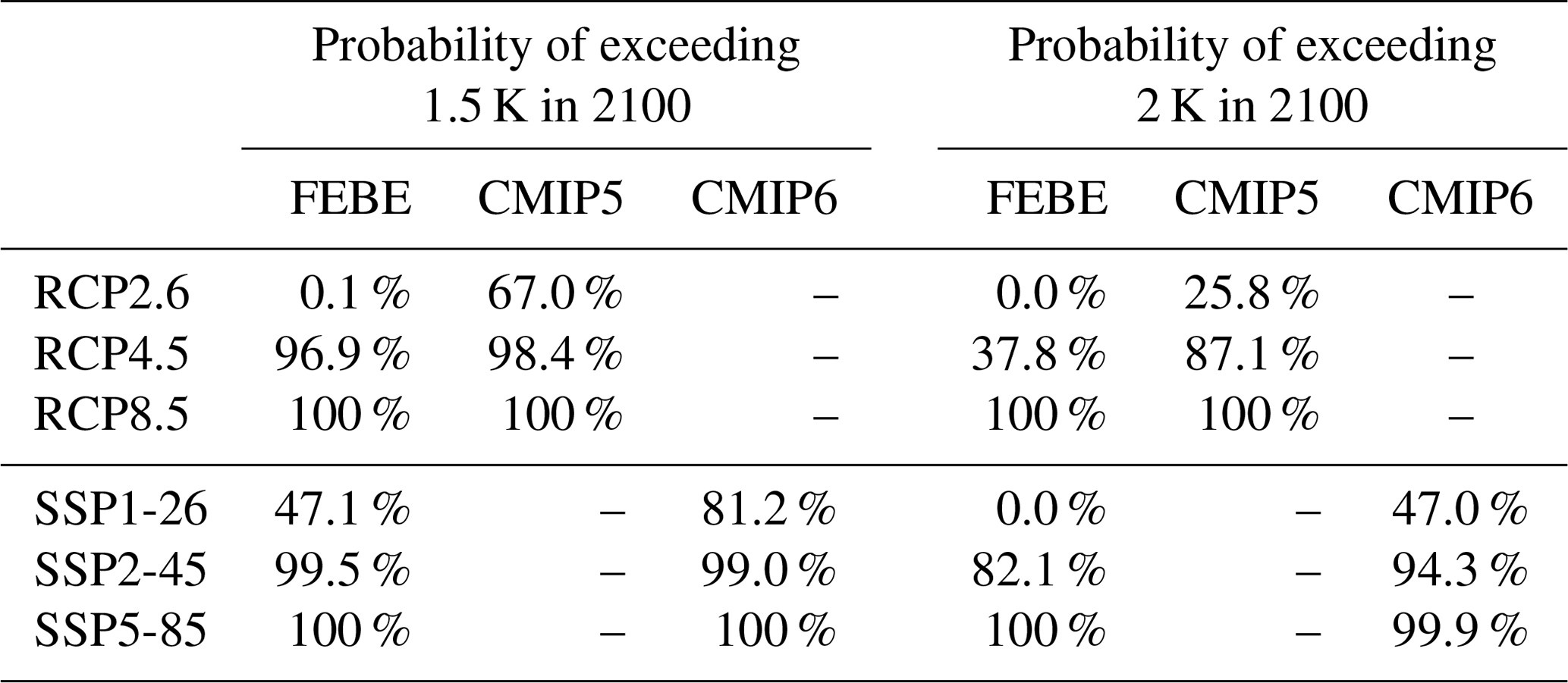
For the final high-emission, business-as-usual, RCP8.5 and SSP5-85 scenarios; both the FEBE and CMIP5/6 MME project that exceeding the 1.5 K threshold is virtually inevitable by 2100, although in the FEBE projection, it is extremely likely that this threshold is exceeded nearly 15 years after the CMIP5/6 MME projections of 2040. The same is found for the 2 K threshold, with both the FEBE and CMIP5/6 MME exceeding the threshold about 15 years after the 1.5 K threshold. These results are all summarized in Table 6.
In the following section, we summarize the key results presented earlier in the paper: model and forcing parameters (see Table 1), the climate sensitivities (see Table 2), the projected warming in 2100 (see Tables 4 and 5) and the probabilities of exceeding warming thresholds of 1.5 and 2.5 K (see Table 6).
6.1 Parameter estimates
The two parameters that characterize the model, h and τ, were estimated. The fundamental scaling exponent h, was found to have a median value of 0.38 and 90 % CI of [0.33, 0.44] using and similar median value 0.38 and 90 % CI of [0.32, 0.44] for . Both estimates are near h estimated for the scaling climate response function (Hébert et al., 2021) and the phenomenological HEBE (Lovejoy, 2021a, b). The relaxation timescale τ, characterizing the approach to equilibrium, was found to have a median value of 4.7 years and 90 % CI of [2.4, 7.0] years when using , and nearly identical results were seen when using . The estimated relaxation time is comparable to other box model fast relaxation times (Schwartz, 2008; Held et al., 2010; Geoffroy et al., 2013; Rypdal and Rypdal, 2014) as the one-box (EBE) model is a special case of the FEBE with h=1.
The FEBE model also adjusts the deterministic forcings, notably the aerosol and volcanic forcing series which must be scaled (the former linearly and the latter non-linearly) for the temperature response to best match historical temperature records. From our analysis, we find a more constrained aerosol forcing. For the , we found a median recalibration factor α of 0.6 with 90 % CI [0.2, 1.0]. Following Stevens (2015), this supports a revision of the global modern (2005) aerosol forcing 90 % CI to a narrower range [−1.0, −0.2] W m−2. Using the CMIP6 aerosols, , we found a median α value of 0.33 and 90 % [0.05, 0.61] implying a weaker and more tightly constrained modern (2005) aerosol forcing of [−0.9, −0.1] W m−2. For volcanism, the non-linear intermittency exponent, ν, was found have median value of 0.28 with 90 % CI of [0.15, 0.41] using and a median 0.28 with similar 90 % CI of [0.16, 0.40] using .
In comparison to IPCC AR5 and to the CMIP6 MME, we find lower likely ranges for the climate sensitivity parameter, ECS and TCR when using the FEBE with (or ). For projections, perhaps the most important parameter is s, the climate sensitivity parameter that determines the temperature response following an increase in forcing. We find s to have a median value of 0.56 K(W m with 90 % CI [0.45, 0.67] K(W using , and when using we find median 0.52 K(W m with 90 % CI [0.43, 0.61] K(W m. Again, we see a lower median for the ECS in comparison to the IPCC AR5 (and CMIP6 MME) estimates for their corresponding forcings, the 90 % CI range is reduced from [1.5, 4.5] K ([2.0, 5.5] K) to [1.6, 2.4] K ([1.5, 2.2] K), and the median value is lowered from 3.0 K (3.7 K) to 2.0 K (1.8 K). Several recent observation-based studies (Otto et al., 2013; Skeie et al., 2014; Johansson et al., 2015; Lewis and Curry, 2015, 2018) have also reported lower ECS upper bounds. We also estimated the derived quantity, the TCR, the temperature increase following a linear doubling in forcing over 70 years. For the TCR, the 90 % CI range shrinks from [1.0, 2.5] K ([1.2, 2.8] K) to [1.2, 1.8] K ([1.1, 1.6] K) and the median estimate decreases from 1.8 K (2.0 K) to 1.5 K (1.4 K).
6.2 Hindcasts
With all necessary parameters of the FEBE calibrated on observational temperature series, we evaluated the FEBE reliability, showing that it is able to reconstruct the historical temperatures (Sect. 4.2), and it can reproduce the response amplitude to a internal white noise forcing (Sect. 4.3) and produces realistic temperature fluctuations over a wide range of scales (Sect. 4.4). Having shown that the FEBE reproduces historical temperatures and their statistics, we then produced deterministic temperature projections to 2100 using the RCP2.6, 4.5, 8.5 and SSP1-26, 2-45, 5-85 comparing them to their respective CMIP5 and CMIP6 MMEs relative to the pre-industrial baseline of 1880–1910.
6.3 Projections
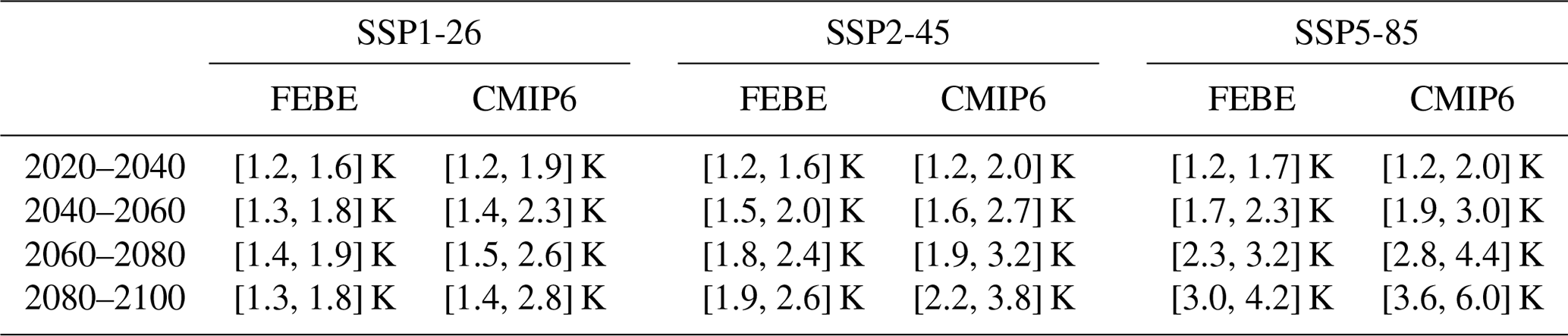
In the low-emission scenario, RCP2.6 (SSP1-26), the FEBE projects the 90 % CI of the temperature in 2100 to be [1.2, 1.6] K ([1.3, 1.8] K) as compared to the CMIP5 (CMIP6) MME of [1.1, 2.4] K ([1.4, 2.8] K). In the middle scenario, RCP4.5 (SSP2-45), the FEBE projects warming reaching [1.6, 2.3] K ([1.9, 2.6] K), narrower than the CMIP5 (CMIP6) MME warming of [1.8, 3.2] K ([2.2, 3.8] K), while in the high-emission scenario, RCP8.5 (SSP5-85), both the FEBE and CMIP5 (CMIP6) MME project extreme temperature increases of [2.7, 3.6] K ([3.0, 4.2] K) and [3.3, 5.3] K ([3.6, 6.0] K), highlighting the need for strong emission mitigation.
During the Paris Conference in 2015 (COP21), nations of the world strengthened the United Nations Framework Convention on Climate Change by agreeing to hold the increase in the global average temperature to well below 2 K above pre-industrial levels and pursuing efforts to limit the temperature increase to 1.5 K. According to our projections, crossing either of these thresholds is delayed with respect to the CMIP5/6 MME projections but will eventually happen if strong mitigation is not implemented. To avert a 1.5 K warming, drastic cuts would have to be made to global greenhouse emissions, similar to that in RCP2.6 (and SSP1-26), for which we found <10 % (<50 %) probability of exceeding 1.5 K in comparison to the CMIP5 (CMIP6) MME, which projects a 67 % (>80 %) increase. Both the FEBE and CMIP5/6 projections have temperatures surpassing 1.5 K in scenarios with weak or no mitigation: RCP4.5/SSP2-45 and RCP8.5/SSP5-85, albeit the FEBE projects this occurring nearly two decades later than the GCMs. The 2 K threshold is projected to be avoided by both the FEBE and CMIP5/6 MME if we follow low-emission scenarios of RCP2.6 and SSP1-26. The opposite is true for any other emission scenarios; exceeding the 2 K threshold will almost occur before 2100. Thus, our model reinforces the conclusion that only strong mitigation scenarios such as RCP2.6 and SSP1-26, will avoid exceeding the 1.5 and 2 K thresholds. It remains to be seen whether negative emission technologies are feasible and whether the appropriate policies are implemented.
Ever since the first climate models in the 1970s, multidecadal projections have had large uncertainties with the wide ECS uncertainty limits of 1.5–4.5 K essentially unchanged. For policymakers, the most deleterious consequence of large uncertainties is that projections emanating from quite diverse future scenarios have significant overlap. For example, up until 2050, the RCP2.6 and 8.5 scenarios can both claim to respect the 2 K threshold – albeit with rather different probabilities (Fig. 13). Large overlaps imply a disconnection between policies (mitigation scenarios) and outcomes (temperatures). Now that governments have committed themselves to keeping industrial epoch temperature increases to below 2 K (and aim at 1.5 K), we face an uncertainty crisis (Lovejoy, 2019).
One way of reducing this uncertainty is by developing complementary types of models. In this paper, we directly constructed such a model in the macroweather regime (roughly 1 month and up) based on the physically principles of energy conservation and scaling: the fractional energy balance equation (FEBE). Although originally derived phenomenologically, it was recently discovered (Lovejoy, 2021a, b) that the FEBE could be derived as a consequence of classical (Budyko, 1969; Sellers, 1969) EBMs that have been regularly used to determine the Earth's latitudinal temperature variations and its stability with perturbations, and to study past and future climate states. The key was to introduce a vertical coordinate that allows for the application of the correct conductive–radiative surface boundary condition, needed for correctly determining the energy storage. A surprising consequence is that even the classical (integer-ordered) continuum mechanics heat equation used by Budyko and Sellers implies that the surface temperature obeys a fractional ordered energy balance equation. The FEBE's fractional storage terms imply that the system has a long memory so that when calibrated by observational data, its responses to past forcings are constrained to respect the historical climate.
The FEBE is a parsimonious model with only two shape parameters: an exponent h and relaxation timescale τ; the classical EBE (box model) is the h=1 special case. In order to make FEBE projections, we use a Bayesian parameter estimation approach similar to that used in Hébert et al. (2021). A climate response function was used by Hébert et al. (2021) that at long times (>τ) was close to the corresponding low-frequency part of the FEBE Green's function but that rather than being truncated at high frequencies was a different power law. While the Hébert et al. (2021) CRF was justified only on the basis of scale invariance and linearity, the FEBE has a stronger physical basis since it respects both scaling as well as energy conservation, and the long memory is explicitly situated in energy storage mechanisms. Beyond its stronger theoretical basis, from the practical (projection) point of view, the main advantage is that the FEBE directly handles the short timescales (down to a month or less). This allows the FEBE to directly take into account the internal variability: a stochastic white noise forcing and the FEBE response. The ability to model the forced response to both external and internal forcing improves the FEBE parameter estimates and contributes to lowering the corresponding projection uncertainties. It also allowed us to demonstrate the projections were reliable (in the technical sense).
Bayesian inference allows for a robust probabilistic parameter characterization. The basic external forcings were those prescribed for the historical part of the CMIP5/6 GCMs and these were constrained by five monthly, global resolution empirical temperature series (since 1880). The internal forcing was assumed to be a Gaussian white noise and, since to a good approximation, the FEBE white noise response is a fractional Gaussian noise (fGn), the latter was taken as the Bayesian inference error model.
In order to estimate the parameters, the forcing series required two adjustments. The most important was the aerosol recalibration parameter α which linearly scales the aerosol forcing to take into account the increasing evidence that the CMIP5 and CMIP6 aerosol cooling was too strong (Padilla et al., 2011; Hébert et al., 2021; Zelinka et al., 2020; Tokarska et al., 2020; Flynn and Mauritsen, 2020). The former aerosol series () was based on uncertain data but also on uncertain modelling assumptions, especially about the direct and indirect effects of aerosols, whereas the latter () is based on global sulfate production and derived from an alternative model than that in CMIP5.
The forcings and parameters combined with the RCP and SSP scenarios allow us to make projections through to 2100; we did this for RCP2.6 (SSP1-26), 4.5 (SSP2-45) and 8.5 (SSP5-85). Overall, the observational-based FEBE projections had uncertainties that are smaller by more than a factor of 2 in comparison to the CMIP5/6 MME uncertainties. However, the two modelling approaches have quite different sources of uncertainty. Whereas the CMIP5/6 uncertainty is purely due to differences in the climates of the GCMs (“structural uncertainties”), the FEBE uncertainty is “parametric” and it depends largely on the uncertainty of the historical forcings and temperatures, in particular those associated with aerosols. In fact, a byproduct of the model and Bayesian framework is that we are able to more tightly constrain aerosol forcing, supporting recent literature findings of weaker historical aerosol cooling. As a consequence, the FEBE projections are consistently a little cooler than those of the CMIP5/6 MME, but with uncertainties about half of those of the MME, it still lies within the MME uncertainty bounds. By comparing the FEBE with the CMIP5 and CMIP6 MMEs, we were also able to separately quantify the contribution of changing the RCP to SSP forcing scenarios from that of the difference in the models. The qualitatively different FEBE thus effectively complements the GCMs.
There is a long history – starting with the four-thirds law of turbulent diffusion (Richardson, 1926) – of attempts to directly stochastically model the collective behaviour of huge numbers of interacting structures and processes. Just as thermodynamics and continuum mechanics are themselves high-level laws with respect to statistical mechanics, stochastic turbulence laws are “high level” with respect to the usual deterministic laws of fluid mechanics. In both cases, the idea is to ignore most of the “details” that turn out to be irrelevant and model only the relevant ones. The FEBE, based on the basic scale and energy symmetries, is a specific contribution to this tradition. It comes at a moment when there is growing interest in stochastic and other alternative approaches to climate modelling and projections (see, e.g. Irrgang et al., 2021).
In addition, whereas the regional (horizontally varying) FEBE has already been derived from the heat equation (Lovejoy, 2021a, b), here it is the greatly simplified “zero-dimensional” (globally averaged) model that is considered (for some early regional FEBE results see e.g. Del Rio Amador and Lovejoy, 2021b; Procyk, 2021). In addition, for simplicity, we restricted the FEBE to the linear case, but it is quite easy to include non-linear model feedbacks – for example, temperature–albedo feedbacks (for glacial–interglacial modelling) or feedbacks such as those from temperature–permafrost emissions relevant to potential tipping points.
In the future, time-varying parameters may also be considered: for example, the climate sensitivity multiplied by the forcing constitutes an “effective forcing” so that time-varying sensitivities are trivial to include – they essentially just change the forcing. Less trivial is the inclusion of time-varying relaxation times, and at the moment it is not obvious that it is possible to even mathematically define a time-varying order of temporal differentiation (i.e. a time-varying h). However, it is possible to use spatially varying h exponents for regional modelling, and this is apparently necessary for regional applications (work in progress and see Del Rio Amador and Lovejoy, 2021a). Other possible directions for generalizing the FEBE include coupling the temperature field with other fields such as precipitation, ice cover, land use and carbon cycle. Finally, it could also be mentioned that various FEBE foundational issues need to be resolved – such as the relationship between top-of-the-atmosphere and surface radiative fluxes – and there also nontrivial practical issues for estimating regional FEBE parameters.
The FEBE, which is an observational model based on energy and scaling symmetries, and its projections to 2100, are complementary to the GCMs. Future work will explore the full (regional, 2-D) FEBE model (Lovejoy, 2021b), which hopefully will constrain and improve future projections. In Lovejoy et al. (2021) and Lovejoy (2021a), the FEBE is shown to plausibly reproduce the annual cycle at monthly resolution, in particular to explain the lag between the temperature maximum and the maximum in the radiative forcing. We can also calibrate the FEBE on the historical runs of the CMIP models in order to perform a feedback analysis to investigate the differences between how models treat their volcanic and aerosol forcings through the parameters ν and α. Updating our parameter estimates from calibrations on GCMs allows for GCM–FEBE hybrid projections. Extensions to precipitation may also be possible at global and regional scales since the FEBE model is consistent with space–time scaling processes in historical precipitation data (de Lima and Lovejoy, 2015). With tighter constraints on ECS and TCR from the FEBE, we can better estimate future warming when bringing together multiple lines of evidence as was done in Sherwood et al. (2020). The FEBE, once expanded spatially, provides a flexible framework which can be calibrated directly on observations, providing a direct representation of forcing to response relationships.
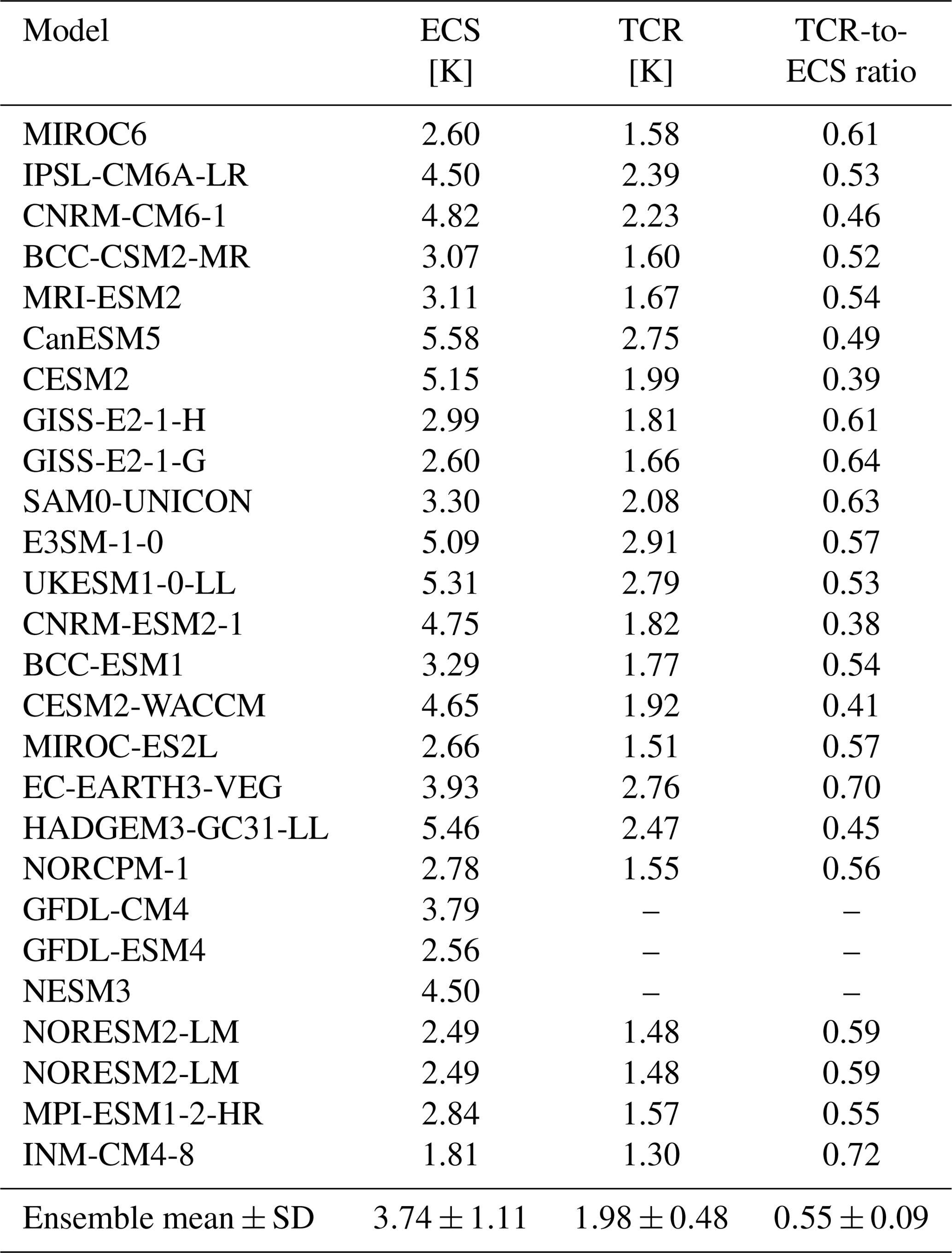
Table A2List of CMIP5 models and climate sensitivity parameters.
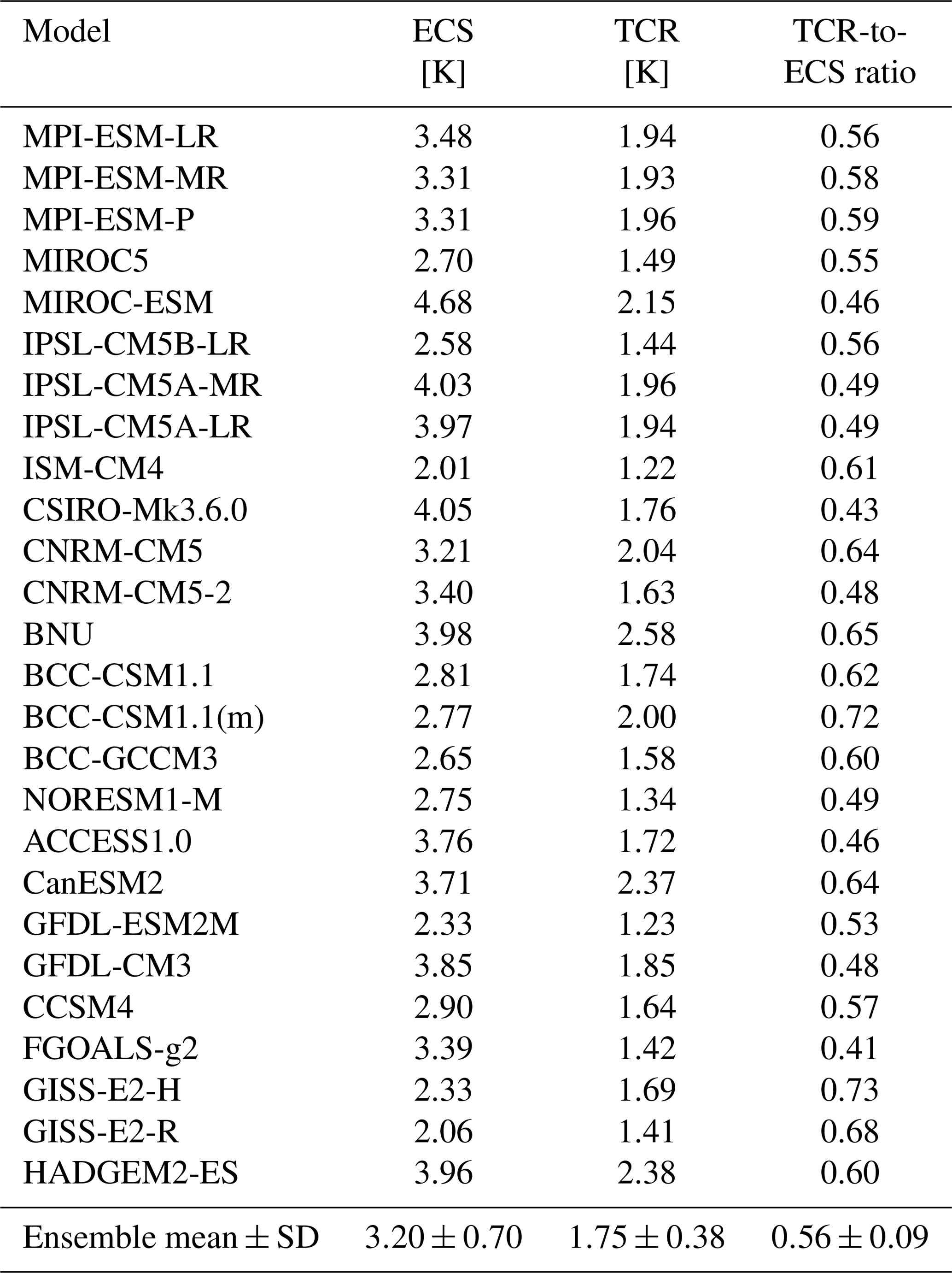
RCP concentrations can be found at https://doi.org/10.1007/s10584-011-0156-z (Meinshausen et al., 2011b). SSP radiative forcings are provided at https://doi.org/10.5281/zenodo.3515339 (Smith, 2019). CMIP5/6 model outputs are available at https://esgf-node.llnl.gov/projects/esgf-llnl/ (ESGF, 2019).
SL was responsible for the conceptualization of the study. RH was responsible for the design of methods for model calibration. RP was responsible for the development the model code and prepared the manuscript with contributions from all co-authors.
The contact author has declared that neither they nor their co-authors have any competing interests.
Publisher's note: Copernicus Publications remains neutral with regard to jurisdictional claims in published maps and institutional affiliations.
Shaun Lovejoy acknowledges some support from the National Science and Engineering research Council (Canada). We thank Dave Clarke and Lenin Del Rio Amador for helpful discussions, and Maya Willard-Stepan for help in editing the manuscript. The work profited from discussions at the CVAS working group of the Past Global Changes (PAGES) programme.
This paper was edited by Valerio Lucarini and reviewed by four anonymous referees.
Raphael Hébert has received funding from the European Research Council (ERC) under the European Union's Horizon 2020 research and innovation programme (grant agreement nos. 716092 and 772852.
Annan, J. D. and Hargreaves, J. C.: Reliability of the CMIP3 ensemble, Geophys. Res. Lett., 37, L02703, https://doi.org/10.1029/2009gl041994, 2010. a
Bellouin, N., Quaas, J., Gryspeerdt, E., Kinne, S., Stier, P., Watson-Parris, D., Boucher, O., Carslaw, K. S., Christensen, M., Daniau, A.-L., Dufresne, J.-L., Feingold, G., Fiedler, S., Forster, P., Gettelman, A., Haywood, J. M., Lohmann, U., Malavelle, F., Mauritsen, T., McCoy, D. T., Myhre, G., Mülmenstädt, J., Neubauer, D., Possner, A., Rugenstein, M., Sato, Y., Schulz, M., Schwartz, S. E., Sourdeval, O., Storelvmo, T., Toll, V., Winker, D., and Stevens, B.: Bounding Global Aerosol Radiative Forcing of Climate Change, Rev. Geophys., 58, e2019RG000660, https://doi.org/10.1029/2019RG000660, 2020. a, b
Bretherton, S.: A National Strategy for Advancing Climate Modeling, The National Academies Press, Washington, DC, https://doi.org/10.17226/13430, 2012. a
Budyko, M. I.: The effect of solar radiation variations on the climate of the Earth, Tellus, 21, 611–619, 1969. a, b
Chan, D. and Huybers, P.: Correcting Observational Biases in Sea-Surface Temperature Observations Removes Anomalous Warmth during World War II, J. Climate, 34, 4585–4602, https://doi.org/10.1175/JCLI-D-20-0907.1, 2021. a
Collins, M., Knutti, R., Arblaster, J., Dufresne, J.-L., Fichefet, T., Friedlingstein, P., Gao, X., Gutowski, W. J., Johns, T., Krinner, G., Shongwe, M., Tebaldi, C., Weaver, A. J., and Wehner, M.: Long-term climate change: Projections, commitments and irreversibility, Cambridge University Press, Cambridge, UK, 1029–1136, https://doi.org/10.1017/CBO9781107415324.024, 2013. a
Cowtan, K. and Way, R.: Update to `Coverage bias in the HadCRUT4 temperature series and its impact on recent temperature trends'. Temperature reconstruction by domain: version 2.0 temperature series, Quarterly Journal of the Royal Meteorological Society, Q. J. Roy. Meteorol. Soc., 140, 1935–1944, https://doi.org/10.1002/qj.2297, 2014a. a
Cowtan, K. and Way, R. G.: Coverage bias in the HadCRUT4 temperature series and its impact on recent temperature trends, Q. J. Roy. Meteorol. Soc. 140, 1935–1944, https://doi.org/10.1002/qj.2297, 2014b. a
Cowtan, K., Hausfather, Z., Hawkins, E., Jacobs, P., Mann, M. E., Miller, S. K., Steinman, B. A., Stolpe, M. B., and Way, R. G.: Robust comparison of climate models with observations using blended land air and ocean sea surface temperatures, Geophys. Res. Lett., 42, 6526–6534, 2015. a
Crowley, T. J., Zielinski, G., Vinther, B., Udisti, R., Kreutz, K., Cole-Dai, J., and Castellano, E.: Volcanism and the little ice age, PAGES News, 16, 22–23, 2008. a
de Lima, M. I. P. and Lovejoy, S.: Macroweather precipitation variability up to global and centennial scales, Water Resour. Res., 51, 9490–9513, https://doi.org/10.1002/2015WR017455, 2015. a
Del Rio Amador, L. and Lovejoy, S.: Predicting the global temperature with the Stochastic Seasonal to Interannual Prediction System (StocSIPS), Clim. Dynam., 53, 4373–4411, https://doi.org/10.1007/s00382-019-04791-4, 2019. a, b, c, d, e, f
Del Rio Amador, L. and Lovejoy, S.: Long-Range Forecasting as a Past Value Problem: Untangling Correlations and Causality With Scaling, Geophy. Res. Lett., 48, e2020GL092147, https://doi.org/10.1029/2020GL092147, 2021a. a, b, c
Del Rio Amador, L. and Lovejoy, S.: Using regional scaling for temperature forecasts with the Stochastic Seasonal to Interannual Prediction System (StocSIPS), Clim. Dynam., 57, 727–756, https://doi.org/10.1007/s00382-021-05737-5, 2021b. a, b
ESGF – Earth System Grid Federation: ESGF Node at DOE/LLNL, Earth System Grid Federation (ESGF), available at: https://esgf-node.llnl.gov/projects/esgf-llnl/, last access: 20 December 2019. a
Flynn, C. M. and Mauritsen, T.: On the climate sensitivity and historical warming evolution in recent coupled model ensembles, Atmos. Chem. Phys., 20, 7829–7842, https://doi.org/10.5194/acp-20-7829-2020, 2020. a, b, c, d
Forest, C. E., Stone, P. H., Sokolov, A. P., Allen, M. R., and Webster, M. D.: Quantifying Uncertainties in Climate System Properties with the Use of Recent Climate Observations, Science, 295, 113–117, https://doi.org/10.1126/science.1064419, 2002. a
Forest, C. E., Stone, P. H., and Sokolov, A. P.: Estimated PDFs of climate system properties including natural and anthropogenic forcings, Geophys. Res. Lett., 33, L01705, https://doi.org/10.1029/2005GL023977, 2006. a
Forster, P. M., Maycock, A. C., McKenna, C. M., and Smith, C. J.: Latest climate models confirm need for urgent mitigation, Nat. Clim. Change, 10, 7–10, https://doi.org/10.1038/s41558-019-0660-0, 2020. a
Geoffroy, O., Saint-Martin, D., Olivié, D. J., Voldoire, A., Bellon, G., and Tytéca, S.: Transient climate response in a two-layer energy-balance model. Part I: Analytical solution and parameter calibration using CMIP5 AOGCM experiments, J. Climate, 26, 1841–1857, 2013. a, b, c
Ghil, M. and Lucarini, V.: The physics of climate variability and climate change, Rev. Mod. Phys., 92, 035002, https://doi.org/10.1103/RevModPhys.92.035002, 2020. a
Gregory, J. M. and Andrews, T.: Variation in climate sensitivity and feedback parameters during the historical period, Geophys. Res. Lett., 43, 3911–3920, 2016. a
Harries, J. E. and Belotti, C.: On the Variability of the Global Net Radiative Energy Balance of the Nonequilibrium Earth, J. Climate, 23, 1277–1290, https://doi.org/10.1175/2009JCLI2797.1, 2010. a
Harvey, L. D. and Kaufmann, R. K.: Simultaneously constraining climate sensitivity and aerosol radiative forcing, J. Climate, 15, 2837–2861, 2002. a
Hasselmann, K.: Stochastic climate models Part I. Theory, Tellus, 28, 473–485, https://doi.org/10.3402/tellusa.v28i6.11316, 1976. a, b
Hébert, R. and Lovejoy, S.: Interactive comment on “Global warming projections derived from an observation-based minimal model” by K. Rypdal, Earth Syst. Dynam., 7, 51–70, https://doi.org/10.5194/esd-7-51-2016, 2015. a
Hébert, R. and Lovejoy, S.: Regional Climate Sensitivity- and Historical-Based Projections to 2100, Geophys. Res. Lett., 45, 4248–4254, https://doi.org/10.1002/2017GL076649, 2018. a
Hébert, R., Lovejoy, S., and Tremblay, B.: An Observation-based Scaling Model for Climate Sensitivity Estimates and Global Projections to 2100, Clim. Dynam., 56, 1105–1129, https://doi.org/10.1007/s00382-020-05521-x, 2021. a, b, c, d, e, f, g, h, i, j, k, l, m, n, o, p, q, r, s, t
Held, I., Winton, M., Takahashi, K., Delworth, T., Zeng, F., and Vallis, G. K.: Probing the Fast and Slow Components of Global Warming by Returning Abruptly to Preindustrial Forcing, J. Climate, 23, 2418–2427, https://doi.org/10.1175/2009JCLI3466.1, 2010. a, b
Huang, B., Menne, M. J., Boyer, T., Freeman, E., Gleason, B. E., Lawrimore, J. H., Liu, C., Rennie, J. J., Schreck, C. J., Sun, F., Vose, R., Williams, C. N., Yin, X., and Zhang, H.-M.: Uncertainty Estimates for Sea Surface Temperature and Land Surface Air Temperature in NOAAGlobalTemp Version 5, J. Climate, 33, 1351–1379, https://doi.org/10.1175/JCLI-D-19-0395.1, 2020. a
Imkeller, P. and Von Storch, J.-S.: Stochastic climate models, in: vol. 49, Birkhäuser, Birkhäuser, Basel, 2001. a
IPCC: Climate Change 2013: The Physical Science Basis, in: Contribution of Working Group I to the Fifth Assessment Report of the Intergovernmental Panel on Climate Change, Cambridge University Press, Cambridge, UK and New York, NY, USA, https://doi.org/10.1017/CBO9781107415324, 2013. a, b, c, d
Irrgang, C., Boers, N., Sonnewald, M., Barnes, E. A., Kadow, C., Staneva, J., and Saynisch-Wagner, J.: Towards neural Earth system modelling by integrating artificial intelligence in Earth system science, Nat. Mach. Intell., 3, 667–674, 2021. a
Iseri, Y., Yoshikawa, S., Kiguchi, M., Tawatari, R., Kanae, S., and Oki, T.: Towards the incorporation of tipping elements in global climate risk management: probability and potential impacts of passing a threshold, Sustainabil. Sci., 13, 315–328, https://doi.org/10.1007/s11625-018-0536-7, 2018. a
Johansson, D. J., O'Neill, B. C., Tebaldi, C., and Häggström, O.: Equilibrium climate sensitivity in light of observations over the warming hiatus, Nat. Clim. Change, 5, 449–453, 2015. a
Kaufmann, R. K., Kauppi, H., Mann, M. L., and Stock, J. H.: Reconciling anthropogenic climate change with observed temperature 1998–2008, P. Natl. Acad. Sci. USA, 108, 11790–11793, https://doi.org/10.1073/pnas.1102467108, 2011. a
Knutti, R., Furrer, R., Tebaldi, C., Cermak, J., and Meehl, G. A.: Challenges in Combining Projections from Multiple Climate Models, J. Climate, 23, 2739–2758, https://doi.org/10.1175/2009JCLI3361.1, 2010. a
Lenssen, N., Schmidt, G., Hansen, J., Menne, M., Persin, A., Ruedy, R., and Zyss, D.: Improvements in the GISTEMP uncertainty model, J. Geophys. Res.-Atmos., 124, 6307–6326, https://doi.org/10.1029/2018JD029522, 2019. a
Lewis, N. and Curry, J. A.: The implications for climate sensitivity of AR5 forcing and heat uptake estimates, Clim. Dynam., 45, 1009–1023, https://doi.org/10.1007/s00382-014-2342-y, 2015. a, b
Lewis, N. and Curry, J.: The Impact of Recent Forcing and Ocean Heat Uptake Data on Estimates of Climate Sensitivity, J. Climate, 31, 6051–6071, https://doi.org/10.1175/JCLI-D-17-0667.1, 2018. a
Lovejoy, S.: What Is Climate?, Eos Trans. Am. Geophys. Union, 94, 1–2, https://doi.org/10.1002/2013EO010001, 2013. a, b
Lovejoy, S.: Using scaling for macroweather forecasting including the pause, Geophys. Res. Lett., 42, 7148–7155, 2015a. a, b
Lovejoy, S.: A voyage through scales, a missing quadrillion and why the climate is not what you expect, Clim. Dynam., 44, 3187–3210, https://doi.org/10.1007/s00382-014-2324-0, 2015b. a, b, c
Lovejoy, S.: Weather, Macroweather and Climate: our random yet predictable atmosphere, Oxford University Press, Oxford, 2019. a, b, c
Lovejoy, S.: The half-order energy balance equation – Part 1: The homogeneous HEBE and long memories, Earth Syst. Dynam., 12, 469–487, https://doi.org/10.5194/esd-12-469-2021, 2021a. a, b, c, d, e, f
Lovejoy, S.: The half-order energy balance equation – Part 2: The inhomogeneous HEBE and 2D energy balance models, Earth Syst. Dynam., 12, 489–511, https://doi.org/10.5194/esd-12-489-2021, 2021b. a, b, c, d, e, f
Lovejoy, S.: Fractional relaxation noises, motions and the fractional energy balance equation, Nonlin. Processes Geophys., https://doi.org/10.5194/npg-2019-39, in press, 2022. a, b, c, d, e
Lovejoy, S. and Schertzer, D.: The Weather and Climate: Emergent Laws and Multifractal Cascades, Cambridge University Press, Cambridge, https://doi.org/10.1017/CBO9781139093811, 2013. a, b, c, d
Lovejoy, S. and Varotsos, C.: Scaling regimes and linear/nonlinear responses of last millennium climate to volcanic and solar forcings, Earth Syst. Dynam., 7, 133–150, https://doi.org/10.5194/esd-7-133-2016, 2016. a, b
Lovejoy, S., del Rio Amador, L., and Hébert, R.: The ScaLIng Macroweather Model (SLIMM): using scaling to forecast global-scale macroweather from months to decades, Earth Syst. Dynam., 6, 637–658, https://doi.org/10.5194/esd-6-637-2015, 2015. a, b, c, d
Lovejoy, S., Del Rio Amador, L., and Hébert, R.: Harnessing Butterflies: Theory and Practice of the Stochastic Seasonal to Interannual Prediction System (StocSIPS), in: Advances in Nonlinear Geosciences, edited by: Tsonis, A., Springer, Cham, 305–355, https://doi.org/10.1007/978-3-319-58895-7_17, 2017. a
Lovejoy, S., Procyk, R., Hébert, R., and Amador, D. R.: The fractional energy balance equation, Q. J. Roy. Meteorol. Soc., 147, 1964–1988, https://doi.org/10.1002/qj.4005, 2021. a, b, c, d, e, f, g
Medhaug, I., Stolpe, M., Fischer, E., and Knutti, R.: Reconciling controversies about the `global warming hiatus', Nature, 545, 41–47, https://doi.org/10.1038/nature22315, 2017. a
Meehl, G., Arblaster, J., Fasullo, J., Hu, A., and Trenberth, K.: Model-based evidence of deep-ocean heat uptake during surface-temperature hiatus periods, Nat. Clim. Change, 1, 360–364, https://doi.org/10.1038/nclimate1229, 2011. a
Meinshausen, M., Raper, S. C. B., and Wigley, T. M. L.: Emulating coupled atmosphere-ocean and carbon cycle models with a simpler model, MAGICC6 – Part 1: Model description and calibration, Atmos. Chem. Phys., 11, 1417–1456, https://doi.org/10.5194/acp-11-1417-2011, 2011a. a
Meinshausen, M., Smith, S. J., Calvin, K., Daniel, S. J., Kainuma, M. L. T., Lamarque, J. F., Matsumoto, J. F., Montzka, S. A., Raper, S. C. B., Riahi, K., Thomson, A., Velders, G. J. M., and van Vuuren, D. P. P.: The RCP greenhouse gas concentrations and their extensions from 1765 to 2300, Climatic Change, 109, 213–241, https://doi.org/10.1007/s10584-011-0156-z, 2011b. a, b, c
Meinshausen, M., Nicholls, Z. R. J., Lewis, J., Gidden, M. J., Vogel, E., Freund, M., Beyerle, U., Gessner, C., Nauels, A., Bauer, N., Canadell, J. G., Daniel, J. S., John, A., Krummel, P. B., Luderer, G., Meinshausen, N., Montzka, S. A., Rayner, P. J., Reimann, S., Smith, S. J., van den Berg, M., Velders, G. J. M., Vollmer, M. K., and Wang, R. H. J.: The shared socio-economic pathway (SSP) greenhouse gas concentrations and their extensions to 2500, Geosci. Model Dev., 13, 3571–3605, https://doi.org/10.5194/gmd-13-3571-2020, 2020. a
Millar, R. J., Otto, A., Forster, P. M., Lowe, J. A., Ingram, W. J., and Allen, M. R.: Model structure in observational constraints on transient climate response, Climatic Change, 131, 199–211, 2015. a
Morice, C. P., Kennedy, J. J., Rayner, N. A., and Jones, P. D.: Quantifying uncertainties in global and regional temperature change using an ensemble of observational estimates: The HadCRUT4 data set, J. Geophys. Res.-Atmos., 117, D08101, https://doi.org/10.1029/2011JD017187, 2012. a
Murphy, D., Solomon, S., Portmann, R., Rosenlof, K., Forster, P., and Wong, T.: An observationally based energy balance for the Earth since 1950, J. Geophys. Res.-Atmos., 114, D17107, 2009. a
Myhre, G., Highwood, E. J., Shine, K. P., and Stordal, F.: New estimates of radiative forcing due to well mixed greenhouse gases, Geophys. Res. Lett., 25, 2715–2718, 1998. a
Myhre, G., Samset, B. H., Schulz, M., Balkanski, Y., Bauer, S., Berntsen, T. K., Bian, H., Bellouin, N., Chin, M., Diehl, T., Easter, R. C., Feichter, J., Ghan, S. J., Hauglustaine, D., Iversen, T., Kinne, S., Kirkevåg, A., Lamarque, J.-F., Lin, G., Liu, X., Lund, M. T., Luo, G., Ma, X., van Noije, T., Penner, J. E., Rasch, P. J., Ruiz, A., Seland, Ø., Skeie, R. B., Stier, P., Takemura, T., Tsigaridis, K., Wang, P., Wang, Z., Xu, L., Yu, H., Yu, F., Yoon, J.-H., Zhang, K., Zhang, H., and Zhou, C.: Radiative forcing of the direct aerosol effect from AeroCom Phase II simulations, Atmos. Chem. Phys., 13, 1853–1877, https://doi.org/10.5194/acp-13-1853-2013, 2013. a
Myrvoll-Nilsen, E., Sørbye, S. H., Fredriksen, H.-B., Rue, H., and Rypdal, M.: Statistical estimation of global surface temperature response to forcing under the assumption of temporal scaling, Earth Syst. Dynam., 11, 329–345, https://doi.org/10.5194/esd-11-329-2020, 2020. a
Nazarenko, L., Rind, D., Tsigaridis, K., Del Genio, A. D., Kelley, M., and Tausnev, N.: Interactive nature of climate change and aerosol forcing, J. Geophys. Res.-Atmos., 122, 3457–3480, https://doi.org/10.1002/2016JD025809, 2017. a
North, G. R.: Theory of Energy-Balance Climate Models, J. Atmos. Sci., 32, 2033–2043, https://doi.org/10.1175/1520-0469(1975)032<2033:TOEBCM>2.0.CO;2, 1975. a
North, G. R. and Kim, K.-Y.: Energy Balance Climate Models, 1st Edn., Wiley, available at: https://www.perlego.com/book/992583/energy-balance-climate-models-pdf (last access: 17 December 2021), 2017. a
North, G. R., Cahalan, R. F., and Coakley Jr., J. A.: Energy balance climate models, Rev. Geophys., 19, 91–121, 1981. a
Otto, A., Otto, F. E. L., Boucher, O., Church, J., Hegerl, G., Forster, P. M., Gillett, N. P., Gregory, J., Johnson, G. C., Knutti, R., Lewis, N., Lohmann, U., Marotzke, J., Myhre, G., Shindell, D., Stevens, B., and Allen, M. R.: Energy budget constraints on climate response, Nat. Geosci., 6, 415–416, https://doi.org/10.1038/ngeo1836, 2013. a
Padilla, L. E., Vallis, G. K., and Rowley, C. W.: Probabilistic Estimates of Transient Climate Sensitivity Subject to Uncertainty in Forcing and Natural Variability, J. Climate, 24, 5521–5537, https://doi.org/10.1175/2011JCLI3989.1, 2011. a, b
Penner, J., Andreae, M., Annegarn, H., Barrie, L., Feichter, J., Hegg, D., Achuthan, J., Leaitch, R., Murphy, D., Nganga, J., and Pitari, G.: Aerosols, their Direct and Indirect Effects, Climate Change 2001: The Scientific Basis, in: Contribution of Working Group I to the Third Assessment Report of the Intergovernmental Panel on Climate Change, World Meteorological Organization United Nations Environment Program, 289–348, 2001. a
Podlubny, I.: Fractional differential equations: an introduction to fractional derivatives, fractional differential equations, to methods of their solution and some of their applications, Elsevier Science, ISBN 9780080531984, 1999. a, b
Procyk, R.: The Fractional Energy Balance Equation: the Unification of Externally Forced and Internal Variability, MS thesis, McGill University, Montreal, Canada, 2021. a
Proistosescu, C., Donohoe, A., Armour, K. C., Roe, G. H., Stuecker, M. F., and Bitz, C. M.: Radiative feedbacks from stochastic variability in surface temperature and radiative imbalance, Geophys. Res. Lett., 45, 5082–5094, 2018. a
Ramaswamy, V., Boucher, O., Haigh, J., Hauglustaine, D., Haywood, J., Myhre, G., Nakajima, T., Shi, G., and Solomon, S.: Radiative Forcing of Climate Change, Cambridge University Press, Cambridge, 349–416, 2001. a, b
Richardson, L. F.: Atmospheric diffusion shown on a distance-neighbour graph, P. Roy. Soc. Lond. A, 110, 709–737, https://doi.org/10.1098/rspa.1926.0043, 1926. a
Ring, M. J., Lindner, D., Cross, E. F., and Schlesinger, M. E.: Causes of the Global Warming Observed since the 19th Century, Atmos. Clim. Sci., 02, 401–415, https://doi.org/10.4236/acs.2012.24035, 2012. a
Rohde, R. A. and Hausfather, Z.: The Berkeley Earth Land/Ocean Temperature Record, Earth Syst. Sci. Data, 12, 3469–3479, https://doi.org/10.5194/essd-12-3469-2020, 2020. a
Rypdal, K.: Global temperature response to radiative forcing: Solar cycle versus volcanic eruptions, J. Geophys. Res.-Atmos., 117, D06115, https://doi.org/10.1029/2011JD017283, 2012. a
Rypdal, M. and Rypdal, K.: Long-Memory Effects in Linear Response Models of Earth's Temperature and Implications for Future Global Warming, J. Climate, 27, 5240–5258, https://doi.org/10.1175/JCLI-D-13-00296.1, 2014. a
Sato, M., Hansen, J. E., McCormick, M. P., and Pollack, J. B.: Stratospheric aerosol optical depths, 1850–1990, J. Geophys. Res., 98, 22987–22994, 1993. a
Sato, Y., Goto, D., Michibata, T., Suzuki, K., Takemura, T., Tomita, H., and Nakajima, T.: Aerosol effects on cloud water amounts were successfully simulated by a global cloud-system resolving model, Nat. Commun., 9, 985, https://doi.org/10.1038/s41467-018-03379-6, 2018. a
Schurer, A. P., Mann, M. E., Hawkins, E., Tett, S. F. B., and Hegerl, G. C.: Importance of the pre-industrial baseline for likelihood of exceeding Paris goals, Nat. Clim. Change, 7, 563–567, https://doi.org/10.1038/nclimate3345, 2017. a
Schwartz, S. E.: Uncertainty in climate sensitivity: causes, consequences, challenges, Energ. Environ. Sci., 1, 430–453, 2008. a
Sellers, W. D.: A global climatic model based on the energy balance of the earth-atmosphere system, J. Appl. Meteorol., 8, 392–400, 1969. a, b
Sherwood, S., Webb, M. J., Annan, J. D., Armour, K., Forster, P. M., Hargreaves, J. C., Hegerl, G., Klein, S. A., Marvel, K. D., Rohling, E. J., Watanabe, M., Andrews, T., Braconnot, P., Bretherton, C. S., Foster, G. L., Hausfather, Z., von der Heydt, A. S., Knutti, R., Mauritsen, T., Norris, J. R., Proistosescu, C., Rugenstein, M., Schmidt, G. A., Tokarska, K. B., and Zelinka, M. D.: An assessment of Earth's climate sensitivity using multiple lines of evidence, Rev. Geophys., 58, e2019RG000678, https://doi.org/10.1029/2019RG000678, 2020. a
Skeie, R. B., Berntsen, T., Aldrin, M., Holden, M., and Myhre, G.: A lower and more constrained estimate of climate sensitivity using updated observations and detailed radiative forcing time series, Earth Syst. Dynam., 5, 139–175, https://doi.org/10.5194/esd-5-139-2014, 2014. a
Smith, C. J.: Effective Radiative Forcing from Shared Socioeconomic Pathways (v0.3.1). Zenodo [data set], https://doi.org/10.5281/zenodo.3515339, 2019. a
Smith, C. J., Forster, P. M., Allen, M., Leach, N., Millar, R. J., Passerello, G. A., and Regayre, L. A.: FAIR v1.3: a simple emissions-based impulse response and carbon cycle model, Geosci. Model Dev., 11, 2273–2297, https://doi.org/10.5194/gmd-11-2273-2018, 2018. a, b, c
Smith, D. M., Scaife, A. A., Hawkins, E., Bilbao, R., Boer, G. J., Caian, M., Caron, L.-P., Danabasoglu, G., Delworth, T., Doblas-Reyes, F. J., Doescher, R., Dunstone, N. J., Eade, R., Hermanson, L., Ishii, M., Kharin, V., Kimoto, M., Koenigk, T., Kushnir, Y., Matei, D., Meehl, G. A., Menegoz, M., Merryfield, W. J., Mochizuki, T., Müller, W. A., Pohlmann, H., Power, S., Rixen, M., Sospedra-Alfonso, R., Tuma, M., Wyser, K., Yang, X., and Yeager, S.: Predicted Chance That Global Warming Will Temporarily Exceed 1.5 ∘C, Geophys. Res. Lett., 45, 11895–11903, https://doi.org/10.1029/2018GL079362, 2018. a
Smith, T. M., Reynolds, R. W., Peterson, T. C., and Lawrimore, J.: Improvements to NOAA’s historical merged land–ocean surface temperature analysis (1880–2006), J. Climate, 21, 2283–2296, 2008. a
Solomon, S.: Climate Change 2007 the physical science basis: contribution of Working Group I to the Fourth Assessment Report of the IPCC, Cambridge University Press, Cambridge, 2007. a
Solomon, S., Plattner, G.-K., and Friedlingstein, P.: Irreversible climate change due to carbon dioxide emissions, P. Natl. Acad. Sci. USA, 106, 1704–1709, https://doi.org/10.1073/pnas.0812721106, 2009. a
Stainforth, D., Allen, M., Tredger, E., and Smith, L.: Confidence, uncertainty and decision-support relevance in climate predictions, Philos. T. Roy. Soc. A, 365, 2145–2161, https://doi.org/10.1098/rsta.2007.2074, 2007. a
Stevens, B.: Rethinking the Lower Bound on Aerosol Radiative Forcing, J. Climate, 28, 4794–4819, https://doi.org/10.1175/JCLI-D-14-00656.1, 2015. a, b, c, d
Stouffer, R. J.: Time scales of climate response, J. Climate, 17, 209–217, https://doi.org/10.1175/1520-0442(2004)017<0209:TSOCR>2.0.CO;2, 2004. a
Taylor, K. E., Stouffer, R. J., and Meehl, G. A.: An overview of CMIP5 and the experiment design, B. Am. Meteorol. Soc., 93, 485–498, 2012. a
Tebaldi, C. and Knutti, R.: The use of the multi-model ensemble in probabilistic climate projections, Philos. T. Roy. Soc. A, 365, 2053–2075, https://doi.org/10.1098/rsta.2007.2076, 2007. a
Tokarska, K. B., Stolpe, M. B., Sippel, S., Fischer, E. M., Smith, C. J., Lehner, F., and Knutti, R.: Past warming trend constrains future warming in CMIP6 models, Sci. Adv., 6, eaaz9549, https://doi.org/10.1126/sciadv.aaz9549, 2020. a, b
Tomassini, L., Reichert, P., Knutti, R., Stocker, T. F., and Borsuk, M. E.: Robust Bayesian Uncertainty Analysis of Climate System Properties Using Markov Chain Monte Carlo Methods, J. Climate, 20, 1239–1254, https://doi.org/10.1175/JCLI4064.1, 2007. a
Trenberth, K. E., Fasullo, J. T., and Kiehl, J.: Earth's Global Energy Budget, B. Am. Meteorol. Soc., 90, 311–324, https://doi.org/10.1175/2008BAMS2634.1, 2009. a
Trenberth, K. E., Fasullo, J. T., and Balmaseda, M. A.: Earth’s energy imbalance, J. Climate, 27, 3129–3144, 2014. a
Wang, Y.-M., Lean, J., and Sheeley Jr., N.: Modeling the Sun's magnetic field and irradiance since 1713, Astrophys. J., 625, 522, https://doi.org/10.1086/429689, 2005. a
Weisheimer, A. and Palmer, T. N.: On the reliability of seasonal climate forecasts, J. Roy. Soc. Interface, 11, 20131162, https://doi.org/10.1098/rsif.2013.1162, 2014. a
Wolfram Research, Inc.: Mathematica, Version 12.2, Champaign, IL, available at: https://www.wolfram.com/mathematica (last access: 15 December 2021), 2020. a
Zelinka, M. D., Myers, T. A., McCoy, D. T., Po-Chedley, S., Caldwell, P. M., Ceppi, P., Klein, S. A., and Taylor, K. E.: Causes of Higher Climate Sensitivity in CMIP6 Models, Geophys. Res. Lett., 47, e2019GL085782, https://doi.org/10.1029/2019GL085782, 2020. a, b, c, d
Zhang, H., Huang, B., Lawrimore, J., Menne, M., and Smith, T. M.: Global Surface Temperature Dataset (NOAAGlobalTemp), Version 4.0, [NOAA Global Surface Temperature Data], https://doi.org/10.7289/V5FN144H, 2019. a
Zhou, C. and Penner, J. E.: Why do general circulation models overestimate the aerosol cloud lifetime effect? A case study comparing CAM5 and a CRM, Atmos. Chem. Phys., 17, 21–29, https://doi.org/10.5194/acp-17-21-2017, 2017. a
Ziegler, E. and Rehfeld, K.: TransEBM v. 1.0: description, tuning, and validation of a transient model of the Earth's energy balance in two dimensions, Geosci. Model Dev., 14, 2843–2866, https://doi.org/10.5194/gmd-14-2843-2021, 2021. a