Rapid attribution analysis of the extraordinary heat wave on the Pacific coast of the US and Canada in June 2021

Towards the end of June 2021, temperature records were broken by several degrees Celsius in several cities in the Pacific Northwest areas of the US and Canada, leading to spikes in sudden deaths and sharp increases in emergency calls and hospital visits for heat-related illnesses. Here we present a multi-model, multi-method attribution analysis to investigate the extent to which human-induced climate change has influenced the probability and intensity of extreme heat waves in this region. Based on observations, modelling and a classical statistical approach, the occurrence of a heat wave defined as the maximum daily temperature (TXx) observed in the area 45–52^∘ N, 119–123^∘ W, was found to be virtually impossible without human-caused climate change. The observed temperatures were so extreme that they lay far outside the range of historical temperature observations. This makes it hard to state with confidence how rare the event was. Using a statistical analysis that assumes that the heat wave is part of the same distribution as previous heat waves in this region led to a first-order estimation of the event frequency of the order of once in 1000 years under current climate conditions. Using this assumption and combining the results from the analysis of climate models and weather observations, we found that such a heat wave event would be at least 150 times less common without human-induced climate change. Also, this heat wave was about 2 ^∘C hotter than a 1-in-1000-year heat wave would have been in 1850–1900, when global mean temperatures were 1.2 ^∘C cooler than today. Looking into the future, in a world with 2 ^∘C of global warming (0.8 ^∘C warmer than today), a 1000-year event would be another degree hotter. Our results provide a strong warning: our rapidly warming climate is bringing us into uncharted territory with significant consequences for health, well-being and livelihoods. Adaptation and mitigation are urgently needed to prepare societies for a very different future.

1 Introduction

During the last days of June 2021, Pacific Northwest areas of the US and Canada experienced temperatures never previously observed, with temperature records broken in multiple cities by several degrees Celsius. Temperatures far above 40 ^∘C (104 ^∘F) occurred on Sunday 27 June to Tuesday 29 June (Fig. 1a and b for Monday) in the Pacific Northwest areas of the US and western provinces of Canada, with the maximum warmth moving from the western to the eastern part of the domain from Monday to Tuesday. The anomalies relative to the daily maximum temperature climatology for the time of year reached 16 to 20 ^∘C (Fig. 1c and d). It is noteworthy that these record temperatures occurred 1 whole month before the climatologically warmest part of the year (end of July, early August), making them particularly exceptional. Even compared to the average annual maximum temperatures in other years independent of the month considered, the recent event exceeds those temperatures by about 5 ^∘C (Fig. 2). Records were shattered in a very large area, including the village of Lytton, where a new all-time Canadian temperature record of 49.6 ^∘C was set on 29 June and where wildfires spread on the following day.

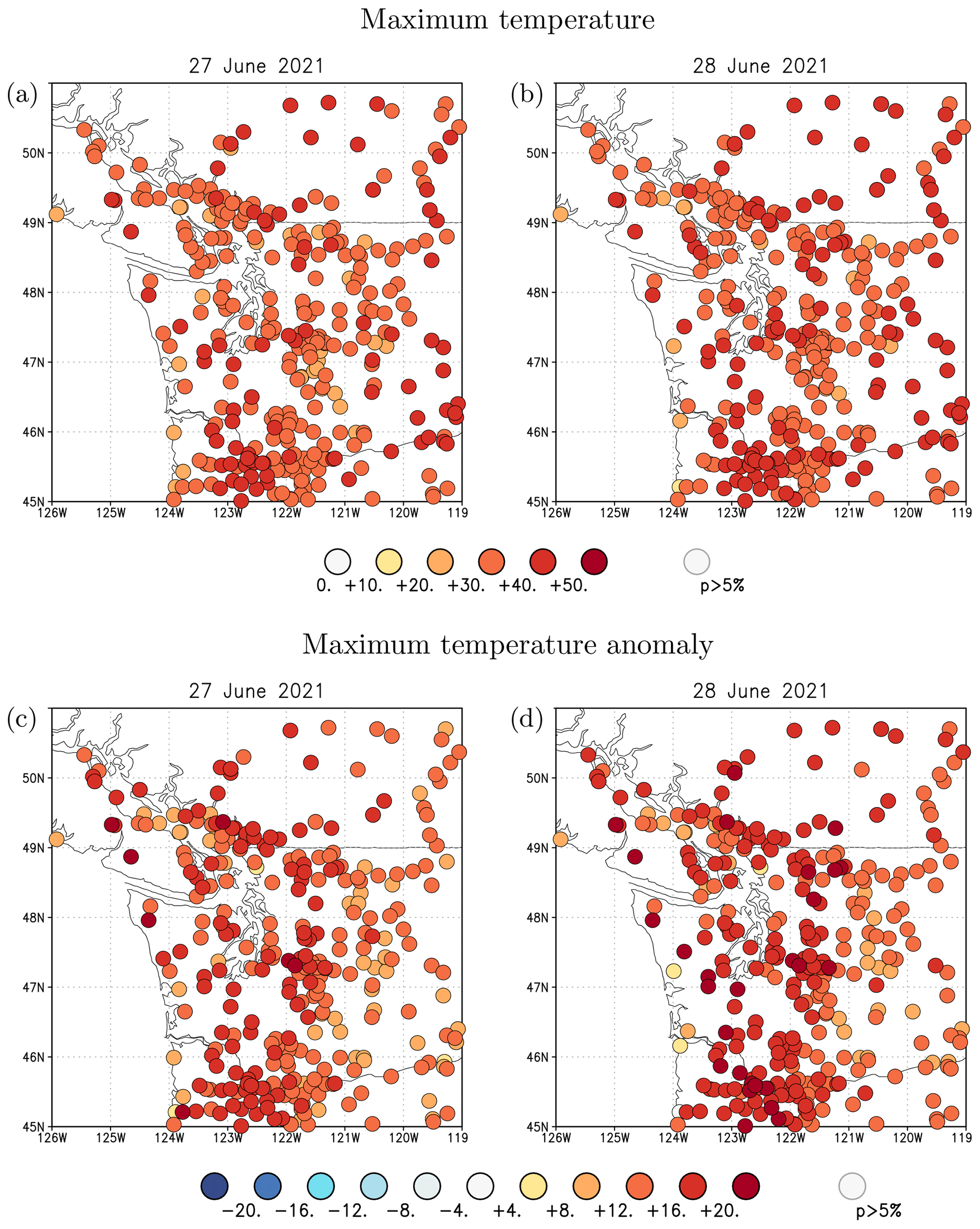
Figure 1 (a) Observed temperatures on 27 June 2021 and (b) 28 June 2021. (c, d) Same for anomalies relative to the climatological mean of the whole station records for these specific days of the year. Source: GHCND (Menne et al., 2012).

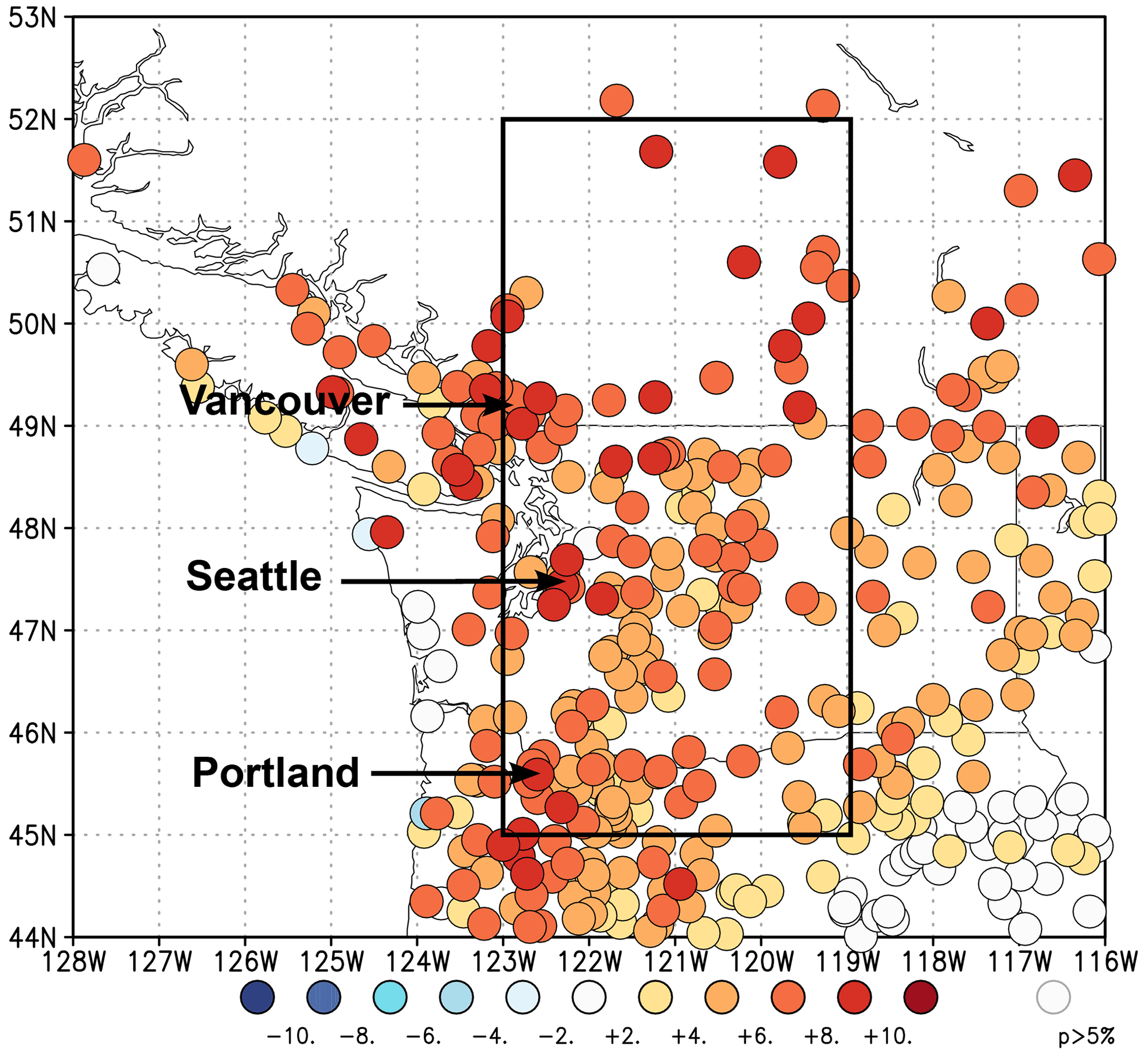
Figure 2 Anomalies of 2021 highest daily maximum temperature (TXx) relative to the mean TXx of the whole time series of each station. The black box indicates the study region. Source: GHCND (Menne et al., 2012).

Given that the observed temperatures were so far outside historical experiences and occurred in a region with only about 50 % household air conditioning penetration, large impacts on health were expected. In British Columbia, Canada, there were an estimated 619 heat-related excess deaths, putting the event among the deadliest weather-related events in Canada (https://www2.gov.bc.ca/assets/gov/birth-adoption-death-marriage-and-divorce/deaths/coroners-service/death-review-panel/extreme_heat_death_review_panel_report.pdf, last access: 22 August 2022). There were an estimated 196 extra deaths in Washington and 100 in Oregon (https://www.opb.org/article/2021/08/06/oregon-june-heat-wave-deaths-names-revealed-medical, last access: 22 August 2022; https://doh.wa.gov/emergencies/be-prepared-be-safe/severe-weather-and-natural-disasters/hot-weather-safety/heat-wave-2021, last access: 22 August 2022).

Below we investigate the role of human-induced climate change in contributing to the likelihood and intensity of this extreme heat wave, following an established approach to multi-model, multi-method extreme-event attribution (Philip et al., 2020; van Oldenborgh et al., 2021). We focus the analysis on the maximum temperatures in the region where most people were affected by the heat (45–52^∘ N, 119–123^∘ W), including the cities of Seattle, Portland and Vancouver. While the extreme heat was an important driver of the observed impacts, it is important to note that these impacts strongly depend on exposure, vulnerability and other climatological variables beyond temperature. In addition to the attribution of the extreme temperatures, we qualitatively assess whether meteorological drivers and antecedent conditions played an important role in the observed extreme temperatures in Sect. 6.

1.1 Event definition

For the attribution analysis, a definition of the event is required. As there are several ways to define an event, this step requires some expert judgement. Within this study, we analyse the daily maximum temperatures, which characterised the event and dominated headlines in a large number of media reports describing the heat wave and its associated impacts. We therefore define the event based on the annual maximum of daily maximum temperature, TXx. Here, we first average over the region and then take the annual maximum. Other options for variables that could be selected for analysis include, for example, 3 d averaged temperatures, as there is some evidence that longer timescales better describe the health impacts (e.g. D'Ippoliti et al., 2010), or high minimum temperatures, which also have strong impacts on human health. However, TXx is a standard heat impact index, and thus the results can easily be compared to other studies. We intentionally focus on one event definition to keep this analysis succinct and its results easy to communicate, choosing TXx, which not only characterises the extreme character of the event but is also readily available in climate models, allowing us to use a large range of different models. Recognising that the World Meteorological Organization (WMO) standard definition of a heat wave is a multi-day measure associated with persistent heat, we additionally considered the annual maxima of 5 and 10 d averages of daily maximum temperatures, TX5x and TX10x, for observations only. Trends in these time series, as seen by the intensity change, turn out to be very similar to the results for TXx presented in Sect. 3. For the spatial scale of the event we consider the area 45–52^∘ N, 119–123^∘ W. This covers the more populated region around Portland, Seattle and Vancouver that was impacted heavily by the heat (with a total population of over 9.4 million in their combined metropolitan areas) but excludes the rainforest to the west and arid areas to the east. Note that this spatial event definition is based on the expected and reported human impacts rather than on the meteorological extremity. Besides the analysis for this region, we also analysed long and homogeneous observational records of three stations in Portland, Seattle and Vancouver.

1.2 Previous trends in heat waves

Figure 3 shows the observed trends in TXx in the GHCN-D dataset over 1900–2019. The stations were selected on the basis of a long time series of at least 50 years of data and were required to be at least 2^∘ apart. The trend is defined as the regression on the global mean temperature, so the numbers represent how much slower or faster the temperature has changed compared to the global mean temperature. Individual stations with different trends to nearby stations usually have inhomogeneities in the observational method or local environment. There are large positive trends in heat waves in Europe. These are not yet fully understood or adequately represented in climate models (Vautard et al., 2020). The negative trends in eastern North America and parts of California are well understood to be the result of land use changes, irrigation and changes in agricultural practice (Donat et al., 2016, 2017; Thiery et al., 2017; Cowan et al., 2020). The Pacific Northwest shows positive trends twice as large as the global mean temperature trend up to  2019.

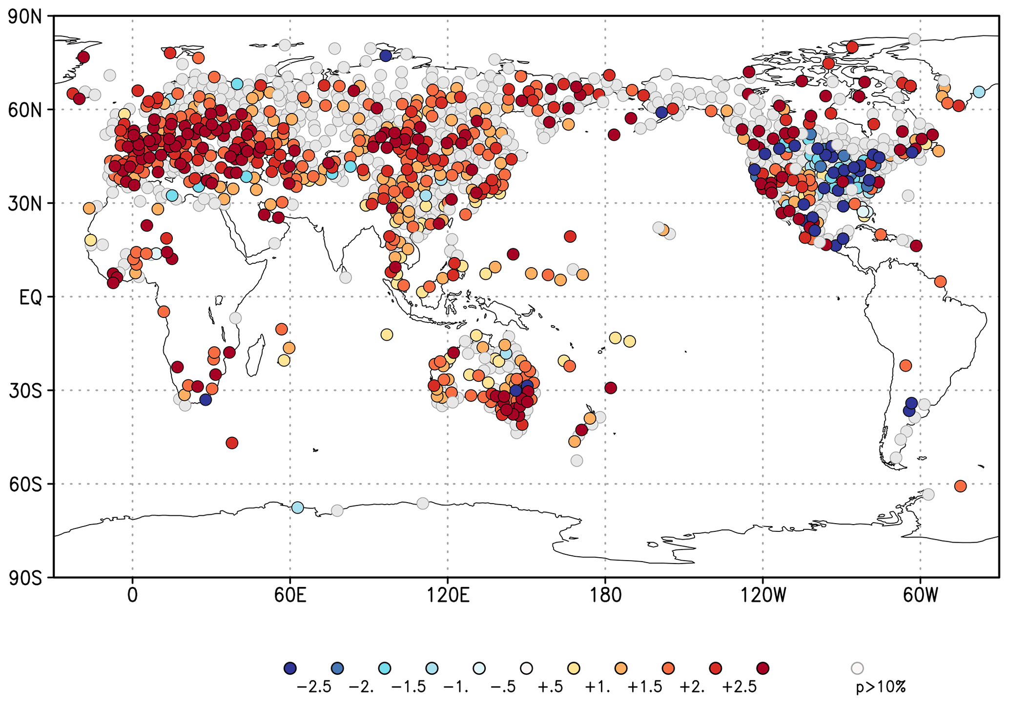
Figure 3 Trends in the highest daily maximum temperature of the year in the GHCN-D station data. Stations are selected to have at least 50 years of data and to be at least 2^∘ apart. The local trends are defined by their regression on the global mean temperature and shown in units of multiples of the global mean temperature rise. Source: GHCND (Menne et al., 2012).

2 Data and methods

2.1 Observational data

The dataset used to represent the heat wave is the ERA5 reanalysis (Hersbach et al., 2019) from the European Centre for Medium-range Weather Forecasts (ECMWF) at 0.25^∘ resolution. A very rapid analysis performed directly after the heat wave and published on https://www.worldweatherattribution.org/western-north-american-extreme-heat-virtually-impossible (last access: 21 April 2022) used ERA5 extended by the ECMWF operational analysis and the ECMWF forecast. The differences in the heat wave amplitude between the rapid analysis and the updated analysis presented here are minor and do not affect the rounded estimate of the return period used in this study. Therefore, the analysis results do not require updating.

Temperature observations were used to assess probability ratios and return periods associated with the event for three major cities in the study area: Portland, Seattle and Vancouver. Observing sites were chosen based on (i) the availability of long homogenised historical records, (ii) their ability to represent the severity of the event by avoiding sites within the proximity of large water bodies and (iii) their representativeness for populous areas of each city to better illuminate impact on inhabitants.

For Portland, the Portland International Airport National Weather Service station was used, which has continuous observations over 1938–2021. The airport is located close to the city centre, adjacent to the Columbia River. The river's influence is thought to be small. For Seattle, Seattle–Tacoma International Airport was chosen, which has almost continuous observations between 1948 and 2021, making it one of the stations with the longest records in the Seattle area. This location is further inland and thus avoids the influence of Lake Washington that affects downtown Seattle. Two long records exist adjacent to downtown Vancouver, but they are both very exposed to the Strait of Georgia that influenced observations due to local onshore flow during the peak of the event. Thus the time series from a site further inland at New Westminster was selected, which starts in 1875 but contains data gaps in 1882–1893, 1928 and 1980–1993.

The data for Portland International Airport and Seattle–Tacoma International Airport were gathered from the Global Historical Climatology Network Daily (GHCND; Menne et al., 2012), while data for New Westminster were gathered from the Adjusted Homogenized Canadian Climate Dataset (AHCCD) for daily temperature (Vincent et al., 2020). This station's record is a composite of data from three locations in two nearby cities as location changes took place in 1966 and 1980. From 1874 to 1966, the station operated at an elevation of 118 m a.s.l. (above sea level) near the centre of New Westminster. In 1966, the station was moved about 2 km east and to an elevation of 18 m. The portion of the homogenised record from 1980 onward is from Pitt Meadows, BC, located about 14 km east of the previous location at an elevation of 5 m. Using a composite station is non-ideal given the potential influence of local micro-climatic effects and particularly the increasing distance from the Strait of Georgia, which exhibits a cooling effect to sites in its vicinity. Use of data from this composite site may increase the uncertainty in our analysis, but given the magnitude of the signal and the consistency of results among the datasets presented here (and analysis of other temperature datasets from BC, not shown here), we do not expect this to substantially affect our results. The AHCCD dataset is updated annually and ends in 2020. Data for 2021 were appended from unhomogenised recent records from Environment and Climate Change Canada. Overlapping data for 2020 were compared between the two sources and found to be identical except for several duplicate/missing observations. Such duplicate or missing data would not cause error in the present analysis because the records are complete for June 2021.

As a measure of anthropogenic climate change we use the global mean surface temperature (GMST), where GMST is taken from the National Aeronautics and Space Administration (NASA) Goddard Institute for Space Science (GISS) surface temperature analysis (GISTEMP; Hansen et al., 2010; Lenssen et al., 2019). We apply a 4-year running mean low-pass filter to suppress the influence of El Niño–Southern Oscillation (ENSO) and winter variability at high northern latitudes as these are unforced variations.

2.2 Model and experiment descriptions

In this study a variety of climate model simulations are analysed and are described in the following paragraphs.

Model simulations from the 6th Coupled Model Intercomparison Project (CMIP6; Eyring et al., 2016) are assessed after combining the historical simulations (1850 to 2014) with the Shared Socioeconomic Pathway (SSP) projections (O'Neill et al., 2016) for the years 2015 to 2100. Here, we only use data from SSP5–8.5, noting that SSPs are very similar over the period 2015–2021. Models are excluded if they do not provide the relevant variables, do not run from 1850 to 2100, or either include duplicate time steps or miss time steps. All available ensemble members are used. A total of 18 models (88 ensemble members) which fulfil these criteria and passed the validation tests (Sect. 4) are used.

In addition an ensemble of extended historical simulations from the IPSL-CM6A-LR model is used (see Boucher et al., 2020, for a description of the model), which follows the CMIP6 protocol (Eyring et al., 2016). It is composed of 32 members, and the simulations cover the historical period (1850–2014). It has been extended until 2029 using all forcings from the SSP2–4.5 scenario, except for the ozone concentration, which has been kept constant at its 2014 climatology, as it was not available at the time the extensions were generated. This ensemble is used to explore the influence of internal variability.

Furthermore we use the GFDL-CM2.5/FLOR model (Vecchi et al., 2014), which is a fully coupled climate model developed at the Geophysical Fluid Dynamics Laboratory (GFDL). While the ocean and ice components have a horizontal resolution of only 1^∘, the resolution of atmosphere and land components is about 50 km and might therefore provide a better simulation than coarser model simulations of certain extreme weather events (Baldwin et al., 2019). The data used in this study cover the period from 1860 to 2100 and combine historical and RCP4.5 experiments driven by transient radiative forcings from CMIP5 (Taylor et al., 2011).

We also examine five ensemble members of the AMIP experiment (1871–2019) from the GFDL-AM2.5C360 (Yang et al., 2021; Chan et al., 2021), which consists of the atmosphere and land components of the FLOR model but with finer horizontal resolution of 25 km for a potentially better representation of extreme events.

Further, we use simulations of the Climate of the 20th Century Plus Project (C20C+), which was designed specifically for event attribution studies (Stone et al., 2019). C20C+ simulations use models of the atmosphere and land with prescribed sea surface temperatures and sea ice concentrations, similar to the design of AMIP experiments. To quantify the impact, if any, on extreme events, participating models were run following the AMIP protocol, and additional sets of counterfactual simulations were performed with anthropogenic influence removed. The distribution of TXx in the study area was examined for three C20C+ models, i.e. CAM5.1, MIROC5 and HadGEM3-A-N216, and compared to that of the ERA5 reanalysis. Only the Community Atmospheric Model (CAM5.1; Neale et al., 2010), run at ∼1^∘ resolution, satisfied the requirements of this study in the statistical description of heat extremes. The actual world ensemble consists of 99 simulations of mixed duration, all ending in 2018, resulting in a sample size of 4090 years. A counterfactual world ensemble of similar size consists of 89 simulations, resulting in a sample size of 3823 years.

2.3 Statistical methods

A more detailed description of the statistical methods is given in Philip et al. (2020) and van Oldenborgh et al. (2021). Here we give a description of the most important aspects.

As discussed in Sect. 1.1, we analyse the annual maximum of daily maximum temperatures (TXx) averaged over 45–52^∘ N, 119–123^∘ W. Initially, we analyse reanalysis data and station data from sites with long data records. Next, we analyse climate model output of TXx. We follow the steps corresponding to the World Weather Attribution (WWA) protocol for event attribution, which for the analysis consist of (i) trend calculation from observations; (ii) model validation; (iii) multi-method, multi-model attribution; and (iv) synthesis of the attribution statement. Steps (i) and (iii) are briefly outlined below, step (ii) is explained in Sect. 4, and we elaborate on step (iv) in Sect. 5

For the event under investigation we calculate the return periods, probability ratio (PR) and change in intensity (ΔT) as a function of GMST, where PR is defined as $\mathrm{PR}=p_{\mathrm{1}}/p_{\mathrm{0}}$, with p₁ the probability of an event as strong as or stronger than the extreme event in the current climate and p₀ the probability of such an event in a counterfactual climate without anthropogenic emissions. The two climates we compared are defined by the GMST of the event year 2021 and a GMST value representative of the climate of the late 19th century, −1.2 ^∘C relative to 2021 (1850–1900, based on the Global Warming Index: https://www.globalwarmingindex.org, last access: 2 July 2021).

To statistically model the selected event, we use a generalised extreme value (GEV) distribution (see e.g. Coles, 2001) that shifts with GMST; i.e. the location parameter has a term proportional to GMST, and the scale and shape parameters are assumed constant. Uncertainties corresponding to the statistical-model uncertainty are obtained using a non-parametric bootstrap procedure. With this GEV distribution, first the PR and intensity change are calculated from observations, as well as the return period in the current climate. Next, the return period is used as a threshold to specify the event magnitude for the models. For this return period, the PRs and intensity changes between 2021 and the counterfactual climate are calculated from different models. This is, however, only done for models that pass our validation tests on the seasonal cycle, the spatial pattern of the climatology, and the scale and shape parameters of the GEV distribution; see Sect. 4. Finally, both observational and model results are synthesised into a consistent attribution statement; see Sect. 5. For models (except IPSL-CM6A-LR and CAM5.1), we additionally analyse the PR between the current climate and a future climate at +2 ^∘C above the 1850–1900 reference, which is equivalent to +0.8 ^∘C above the current climate of 2021. For this analysis of future change we use model data up to about 2050 or when the model GMST reaches +0.8 ^∘C compared to now.

The CMIP6 data are analysed using the same statistical models as the main method. However, for practical reasons, the parameter uncertainty is estimated in a Bayesian setting using a Markov chain Monte Carlo (MCMC) sampler instead of a bootstrapping approach (see Ciavarella et al., 2021, for another example of its application).

3 Observational analysis: return period and trend

Time series of various aspects of the main index are shown in Fig. 4: (a) the daily maximum temperature (Tmax) evolution from ERA5 (from 1 May to 31 August) and (b) annual maximum of Tmax – the index series. The value for 2021, 39.7 ^∘C, is 5.7 ^∘C above the previous record of 34.0 ^∘C. This extremely large increase leads to difficulties in the statistical analysis described below. There are two possible sources of this extreme jump in peak temperatures. The first is that an event with very low probability occurred – the statistical equivalent of “really bad luck”. An event with very low probability could also have occurred in the pre-industrial climate, but its amplitude would have been increased by climate change in the current climate, which already includes about 1.2 ^∘C of global warming. The second option is that strong nonlinear interactions and feedbacks took place in this event, amplifying the intensity of the extreme. This would mean that climate change is acting to exacerbate extreme heat waves more rapidly than implied by a GEV with a location parameter which scales linearly with GMST. In this case, the event would not belong to the “same population” as the other ones, and we would not expect the method applied here to be successful. This second possibility requires further investigation. While we keep this possibility in mind, we assume the first option within this study.

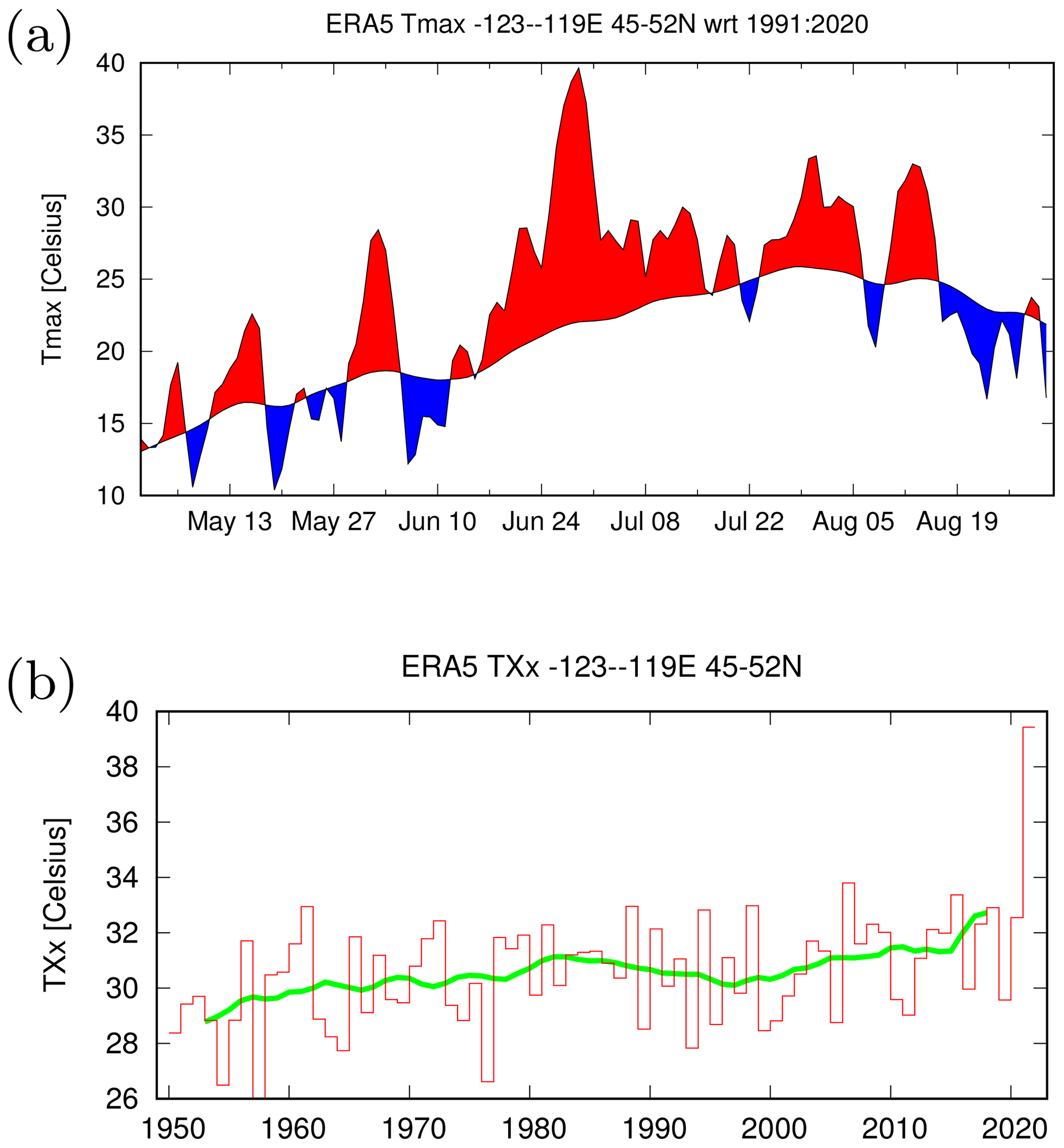
Figure 4 (a) Time series for May–August 2021 of the maximum daily temperature averaged over the study area based on ERA5, with positive and negative departures from the 1991–2020 climatological mean of daily maximum temperature shaded red and blue, respectively. (b) Annual maximum of the index series with a 10-year running mean (green line). Source: ERA5 (Hersbach et al., 2019).

In Fig. 5a we show the seasonal cycle of the daily maximum temperature averaged over the index region, and in Fig. 5b we show the spatial pattern of TXx averaged over many years at each grid point individually. These two metrics are used in the model validation procedure; see Sect. 4.

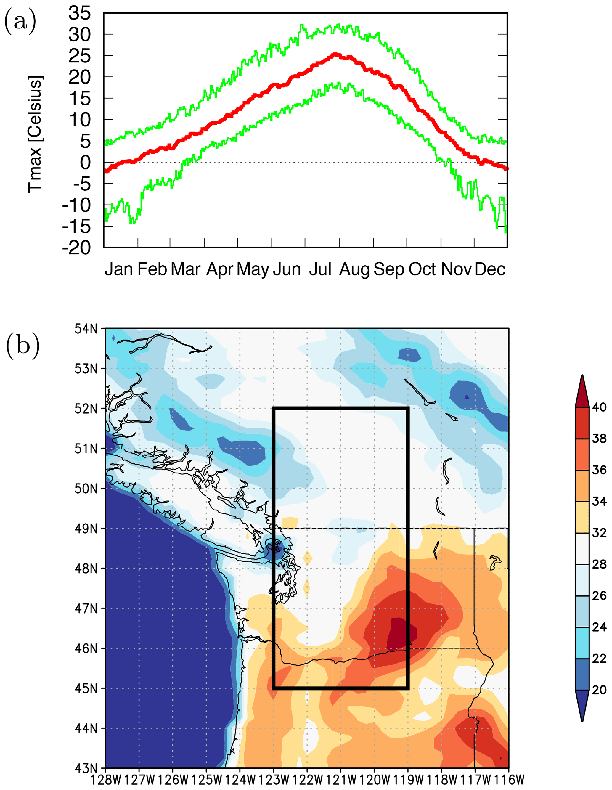
Figure 5 (a) Seasonal cycle of Tmax averaged over the land points of 45–52^∘ N and 119–123^∘ N, showing the 1950–2021 mean (red) and 2.5 % and 97.5 % percentiles of the distribution (green). (b) Spatial pattern of the 1950–2021 mean of the annual maximum of Tmax (multi-year mean TXx) at each grid point. Source: ERA5 (Hersbach et al., 2019).

3.1 Analysis of station and gridded data

Figure 6 shows the analysis of the gridded (ERA5) data using the ordinary extreme value analysis applied for attribution studies within WWA. This approach excludes data of the extreme event of interest from the statistical fit to avoid selection bias, especially when the study area has been defined based on the extent of the extreme event. Figure 6a shows the observed TXx as a function of smoothed GMST and shows that the value observed in 2021 is far outside the range of any values observed to date. The distribution of TXx including data up to 2020 is described very well by a GEV distribution that has linearly warmed at a rate about twice as fast as the GMST; see Fig. 6b. The warming rate is consistent with expectations, as summer temperatures over continents increase faster than the global mean. The GEV fit has a negative shape parameter ξ, which implies a finite tail and hence an upper bound, here at about 35.5±1.3 ^∘C (2σ uncertainty). However, the value observed in 2021, 39.7 ^∘C, is far above this upper bound. Therefore, this GEV fit with constant shape and scale parameters that excludes all information about 2021 does not provide a valid description of heat waves in the area.

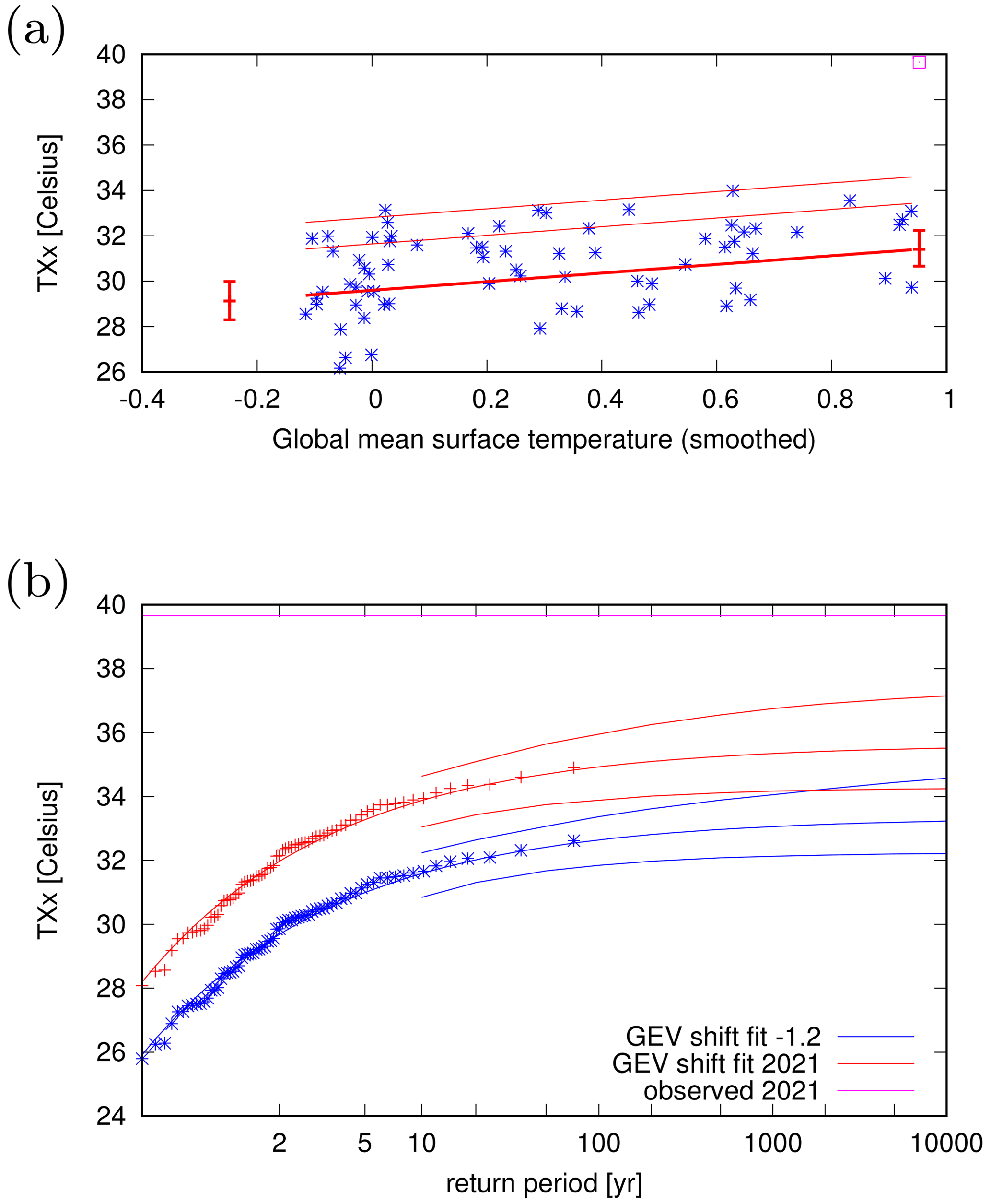
Figure 6 GEV fit with constant scale and shape parameters and location parameter shifting proportional to GMST of the index series. No information from 2021 is included in the fit. (a) The observed TXx as a function of the smoothed GMST. The thick red line denotes the location parameter, the thin red lines the 6- and 40-year return period levels. The June 2021 observation is highlighted with the magenta square and is not included in this fit. (b) Return period plots for the climate of 2021 (red) and a climate with GMST 1.2 ^∘C cooler (blue). The red and blue lines indicate the best fit and the 95 % confidence intervals; the magenta line shows the observed value. The past observations are shown twice: once shifted up to the current climate and once shifted down to the climate of the late 19th century. Source: ERA5 (Hersbach et al., 2019); fit: KNMI Climate Explorer (https://climexp.knmi.nl, last access: 22 April 2022).

An alternative to the standard approach for which no information of the event under study is used (to avoid a selection bias) is to use the information that it actually happened, yet without including the value observed in 2021 in the fit. Specifically, we again assume that the data up to 2020 can be described by a GEV distribution with constant scale and shape parameters, but we reject all GEV models in which the upper bound is below the value observed in 2021. In other words, we enforce that the fit parameters are within a subset of parameters that are compatible with the 2021 event. The result is shown in Fig. 7. While the distribution now includes the 2021 event, the fit to the data up to and including the year 2020 is noticeably worse than when not taking 2021 into account. The return period for the 2021 event under these assumptions still has a lower bound of 10 000 years in the current climate. The fit differs from the previous one mainly in the shape parameter, which is now much less negative (about −0.2 instead of −0.4). This shifts the upper bound to higher values. The fit also gives a somewhat higher trend parameter.

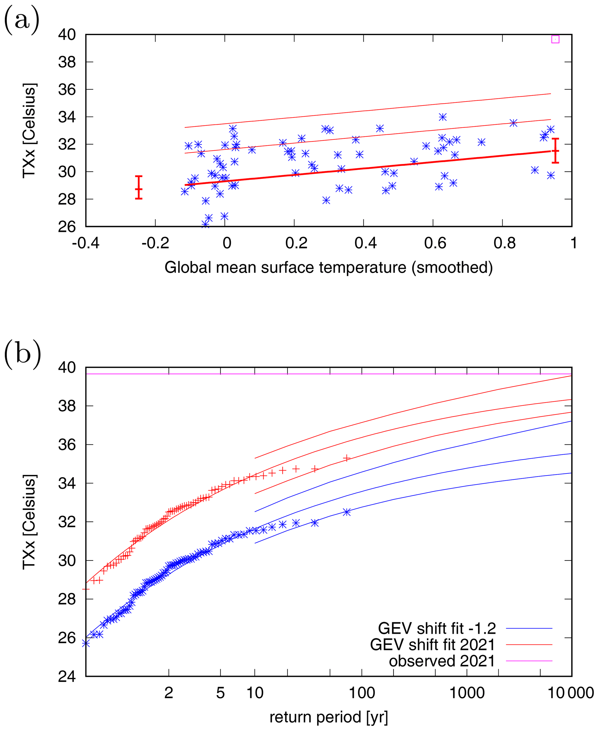
Figure 7 As Fig. 6, but demanding the 2021 event is possible in the fitted GEV function; i.e. the upper bound is higher than the value observed in 2021.

The third possibility is to fit the GEV distribution over all available data, including observations from 2021 (see Fig. 8). This approach implicitly assumes that the 2021 event is drawn from the same population. We typically do not make this assumption in cases where we intentionally select a specific region in order to maximise the extremity (i.e. return period) of the event to avoid a selection bias. Note however that we may have overestimated the return period by excluding the event, a question left for future investigations. In intentionally choosing the region with the largest (rarest) return period for the 2021 event, the extreme value is drawn from a different distribution and cannot be included. However, this is only partly the case here. We did choose the general region because the temperatures were exceptional there; however, we based the choice of subregion for the analysis on population density and type of terrain – parameters that are independent of the heat wave. The benefit of this approach is that it uses all available information. With this approach we still assume this was an event happening by chance; that is, the behaviour is in line with that of a chaotic deterministic system, and by chance we observe a low-probability event in this short time series.

Figure 8 As for Fig. 6 but including data from the 2021 heat wave into the fit.

Given the extremity of the event and the relatively low number of data, a robust GEV fit is hard to obtain, and the appropriateness of the method is difficult to assess. However, the application of this classical method in this case is interesting provided we keep in mind the assumptions we make. While we acknowledge that none of the three possibilities of fitting a GEV distribution is fully satisfying, we decided on using this third approach to estimate the return period leading to an estimate of 1000 years (95 % CI > 100 years; CI: confidence interval). Follow-up research will be necessary to investigate the potential reasons for this exceptional event and the consequences for assumptions for these fits (see also the discussion in Sects. 6 and 8). Also, further research is needed into the limitations of standard GEV analysis on annual maxima with short records and very extreme values. Climate model large ensembles offer a future test bed to investigate the robustness of the method in light of current limitations.

The fit including observations from 2021 (see Fig. 8) gives a 95 % CI of 1.4 to 1.9 K for the scale parameter σ and −0.5 to 0.0 for the shape parameter ξ. These values are used for the model validation in Sect. 4.

The observational analysis results, i.e. the comparison of the fit for 2021 and for a pre-industrial climate, show an increase in intensity of TXx of ΔT=3.1 ^∘C (95 % CI: 1.2 to 4.8 ^∘C) and a probability ratio PR of 390 (3.2 to ∞).

3.2 Analysis of temperature in Portland, Seattle and Vancouver

To represent Portland we chose the International Airport station, which is located on the northern edge of the city and has been collecting data since April 1938; the data are in the GHCN-D v2 database. Figure 9 (top panel) shows the annual maxima of the Portland station time series. The record before 2021 was 41.7 ^∘C in 1965 and 1981, and TXx reached 46.7 ^∘C in 2021, so the previous record was broken by 5.0 ^∘C.

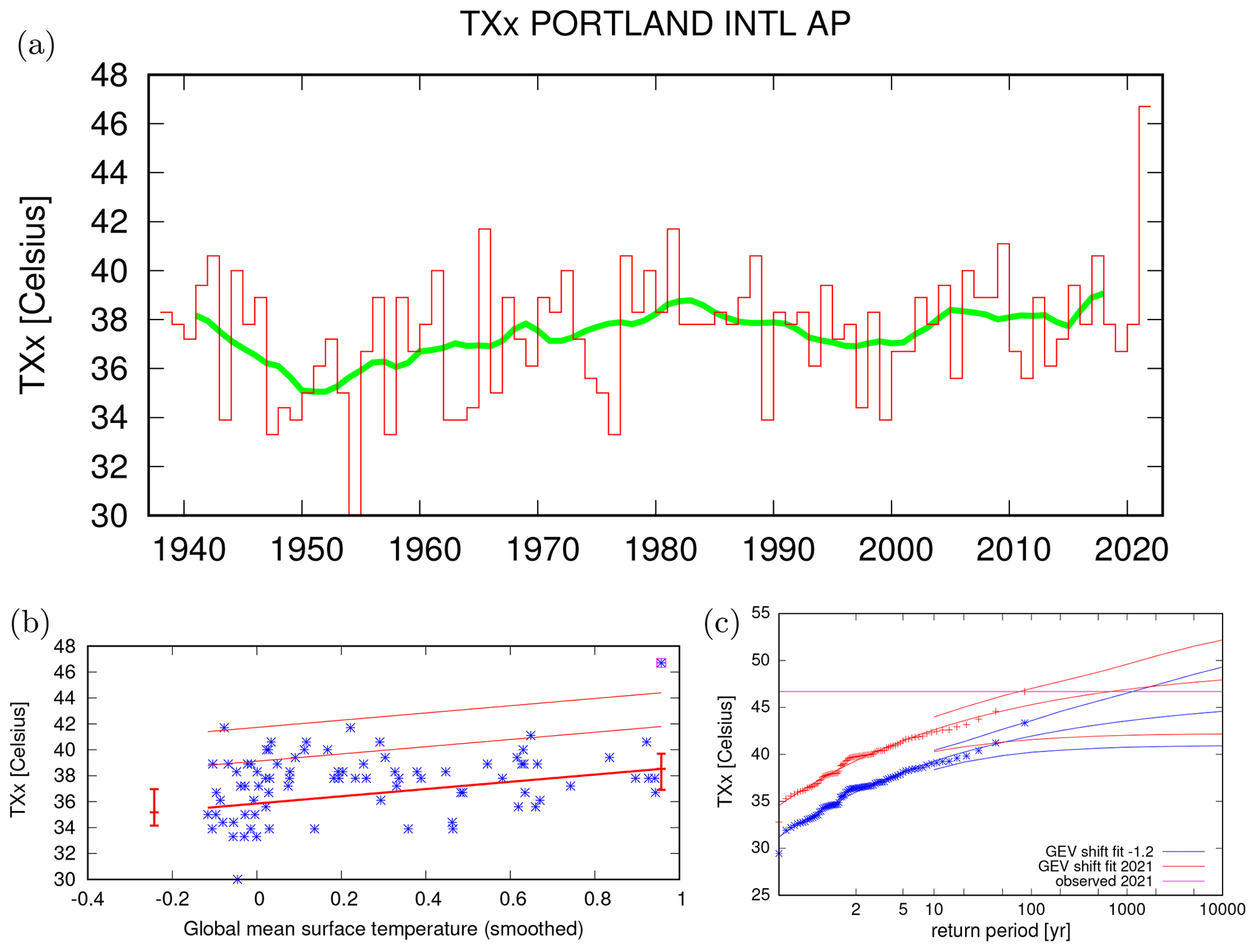
Figure 9 (a) Time series of observed highest daily maximum temperature of the year at Portland International Airport. (b, c) As Fig. 8 but for the station data at Portland International Airport. Source: data GHCN-D (Menne et al., 2012); fit: KNMI Climate Explorer (https://climexp.knmi.nl, last access: 22 April 2022).

We fit a GEV distribution to this data, including 2021 (Fig. 9, lower panels). It gives a return period of 700 years for the 2021 event with a lower bound of 70 years. For the PR we can only give a lower bound (6), since the best estimate is infinite. This corresponds to an increase in TXx of 3.4 ^∘C with a large uncertainty of 0.3 to 5.3 ^∘C. The large uncertainties are due to the somewhat shorter time series and large variability at this station.

In Seattle, the only station with a sufficiently long time series that includes 2021 is Seattle–Tacoma International Airport. It is located ∼15 km south of the city but has similar terrain, without the proximity to water of the city itself. The previous record was 39.4 ^∘C in 2009, and in 2021 it reached 42.2 ^∘C. This is still a large increase of 2.8 ^∘C over the previous record. The event was also not quite as improbable, with a return period of 300 years (lower bound of 40 years) in the current climate (Fig. 10). The PR is again infinite, with a lower bound of 7, and the increase in temperature from a late-19th-century climate is 3.8 ^∘C (0.7 to 5.7 ^∘C).

Figure 10 As Fig. 9 but for the station data at Seattle–Tacoma International Airport.

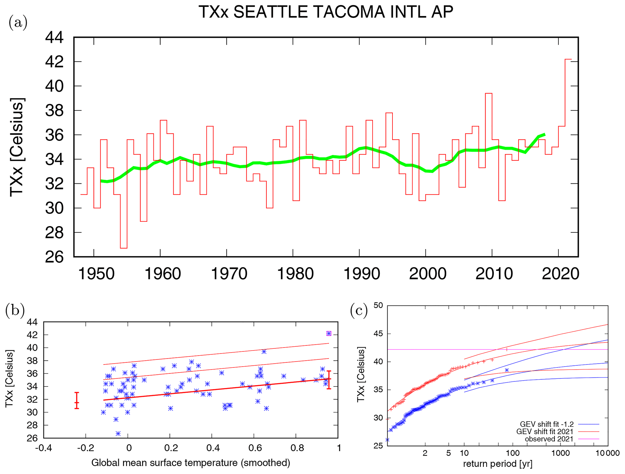
In the Vancouver area, the most representative station with the fewest missing data is New Westminster. It has data from 1875 to 2021 with a few gaps. The previous record was 37.6 ^∘C in 2009, and in 2021 a temperature of 41.4 ^∘C was observed – 4.0 ^∘C warmer. A GEV fit including 2021 gives a return period of 1000 years with a lower bound of 70 years (Fig. 11). The PR is infinite, with a lower bound of 170, and the temperature increased by 3.4 ^∘C (1.9 to 5.5 ^∘C).

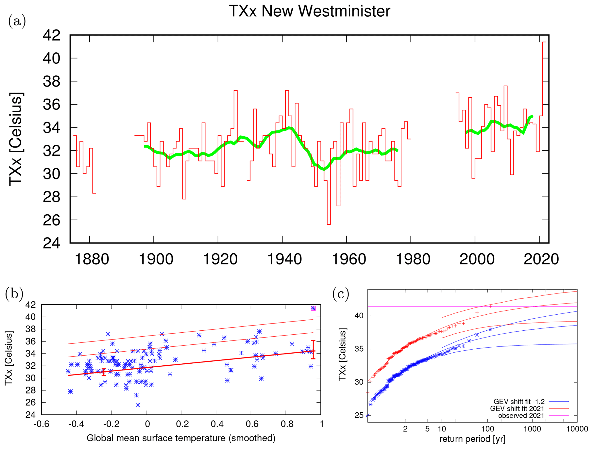
Figure 11 As Fig. 9 but for the station data at New Westminster. Data source: AHCCD (Vincent et al., 2020).

4 Model evaluation and analysis

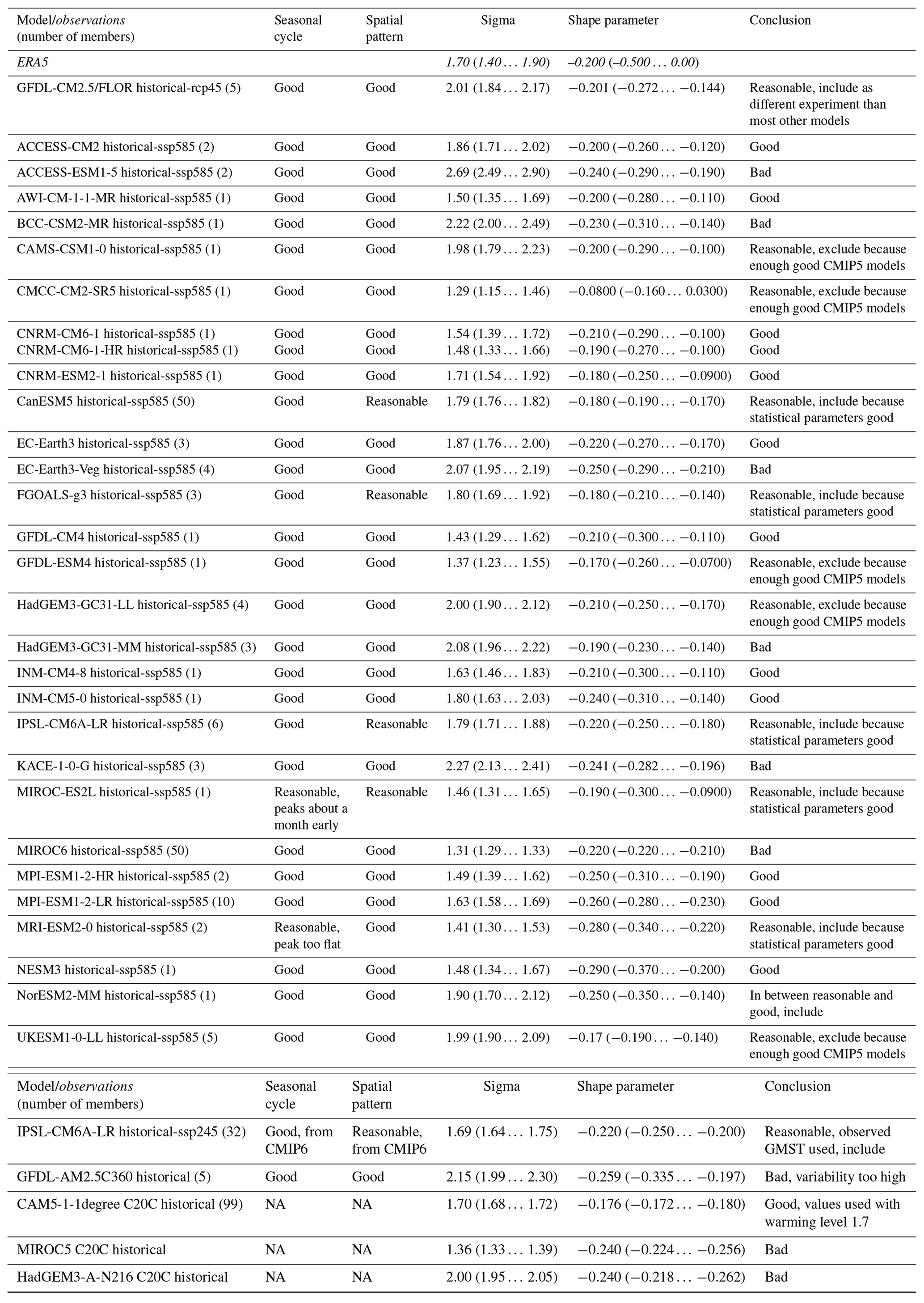
In this section we show the results of the model validation. The validation criteria assess the similarity between the modelled and observed seasonal cycle, the spatial pattern of the climatology, and the scale and shape parameters of the GEV distribution. The assessment results in a label “good”, “reasonable” or “bad”, according to the criteria defined in Ciavarella et al. (2021). In this study, we use models that are labelled “good” or “reasonable”. However, if five or more models are classified as “good” within a particular model set such as the CMIP6 models, then we do not include all of the “reasonable” models but only those that pass the specific test on fit parameters as “good”. Table 1 shows the model validation results. Table A1 includes the models that did not pass the validation tests. In total 21 models and a combined 224 ensemble members passed the validation tests.

Table 1 Validation results for models that passed the validation tests on seasonal cycle, spatial pattern, and fitted GEV scale parameter and shape parameter (σ). Observations in italic.

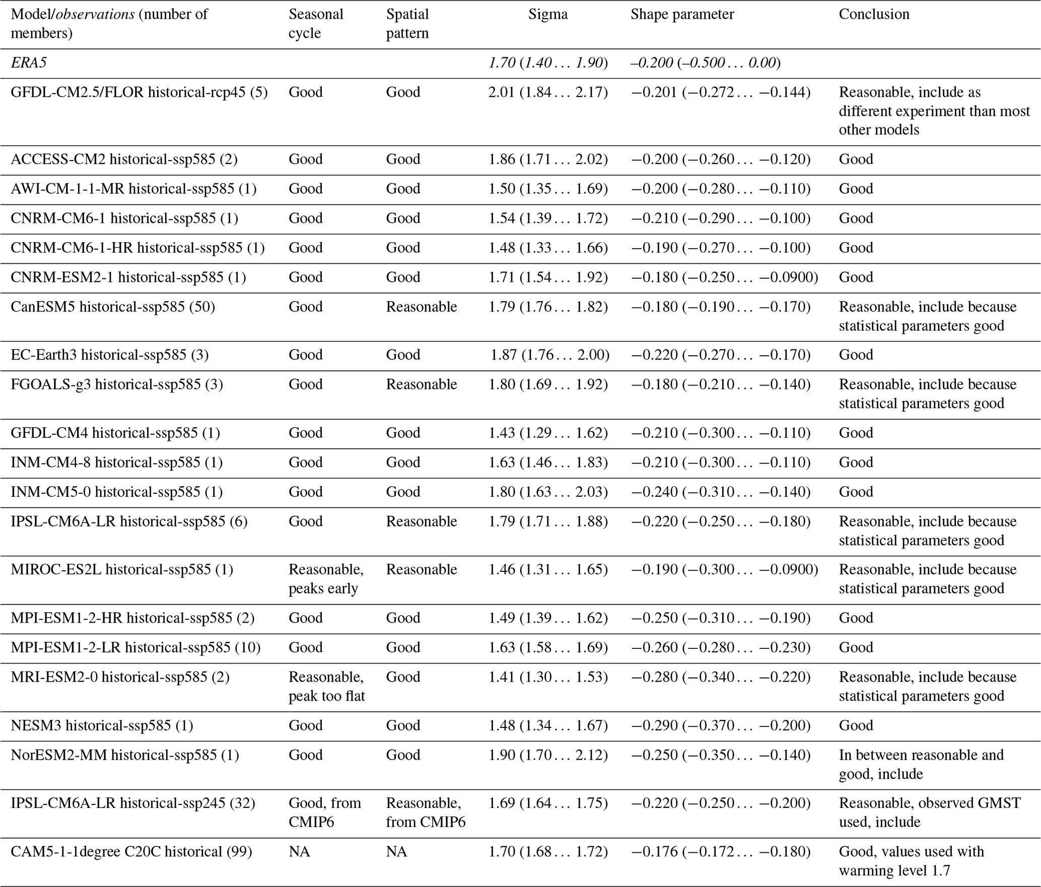
NA stands for “not available”.

Next, we show probability ratios and change in intensity ΔT for models that pass the validation tests, and we also include the threshold values for a 1-in-1000-year event (Table 2). Results are given for both changes in the current climate (1.2 ^∘C) compared to the past (pre-industrial conditions) and, when available, for a climate at +2 ^∘C of global warming above pre-industrial climate compared with the current climate. The results are visualised in Sect. 5.

Table 2 Analysis results showing the model threshold for a 1-in-1000-year event in the current climate and the probability ratios and intensity changes for the present climate with respect to the past (labelled “past”) and for the +2 ^∘C GMST future climate with respect to the present (labelled “future”).

5 Hazard synthesis

In Sects. 3 and 4 we calculated the probability ratio as well as the change in magnitude of the event in the observations and the models. In this section we combine these results to give an overarching synthesised attribution statement and present the results in Figs. 12 and 13. The uncertainty due to differences in model set-up and physics is represented by model spread – the average departure of each model from the mean model best estimate. This is added in quadrature to the model natural variability as white extensions to the light-red bars in the synthesis figures. The uncertainty in the model average (bright-red bar) consists of a weighted mean uncertainty, where the contribution from each model is inversely proportional to the uncertainty due to natural variability squared, plus the model spread term added in quadrature to the uncertainty in the weighted mean. Please see Kew et al. (2021), for example, for more detailed information on the synthesis technique, including how weighting is calculated for models. Observations and the model average are combined into a single result in two ways. Firstly, we compute the weighted average of models and observations: this is indicated by the magenta bar; see Fig. 12. The weighting applied is the inverse square of the uncertainty (the width of the bright bars). Secondly, as there may be an additional model bias that is common to each model (and therefore cannot be detected from the spread of the models), we also show the more conservative estimate of an unweighted average of observations and the model average. This will partly correct for a common model bias, if the observations are reliable, and is indicated by the white box accompanying the magenta bar in the synthesis figures.

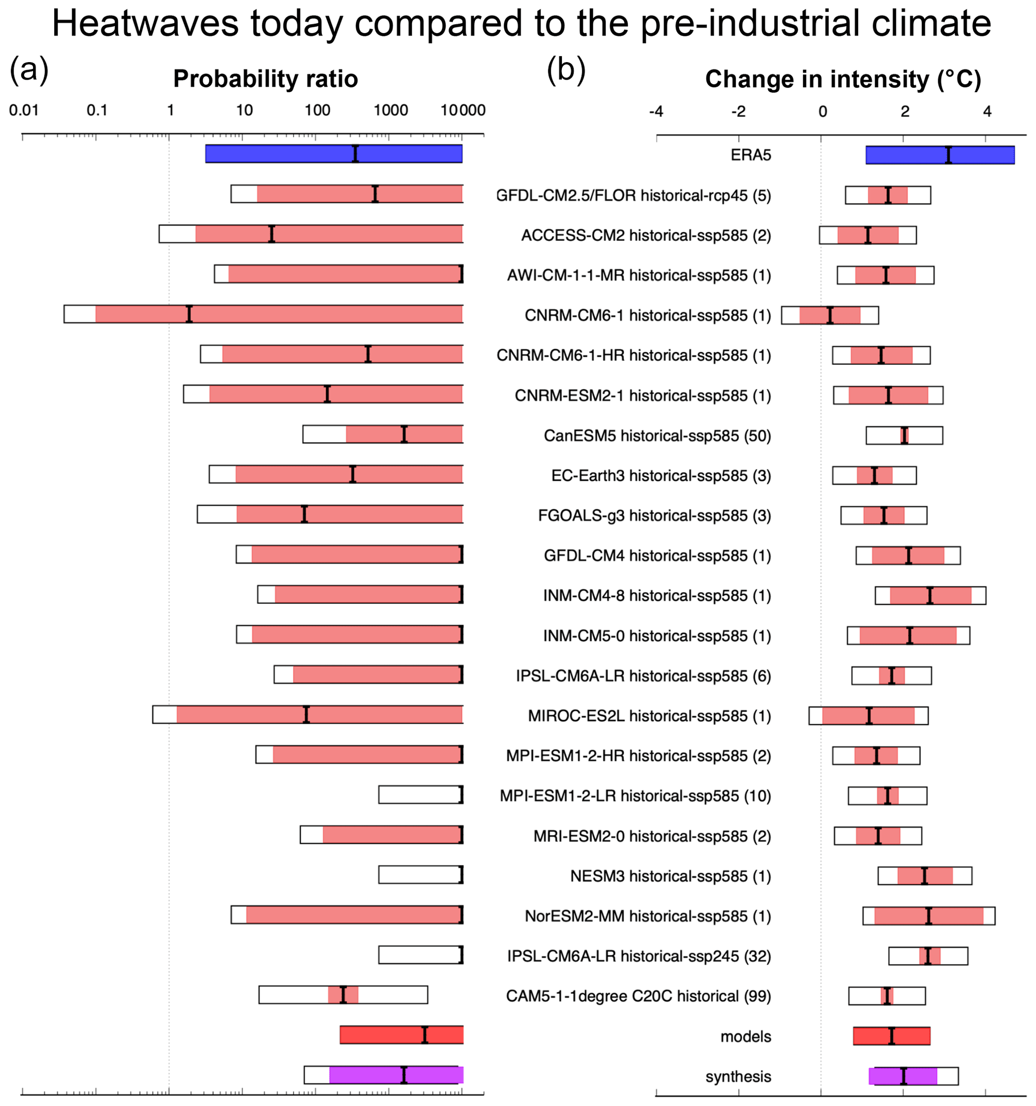
Figure 12 Synthesis of the past climate, showing probability ratios (a) and changes in intensity in degrees Celsius (b), comparing the 2021 event with a pre-industrial climate. The blue bars show ERA5 results, the light-red bars the model results, with model uncertainty shown as white bars around them. The model average is shown by the bright-red bars. The magenta bars are the synthesised values, and the white box accompanying the magenta bar indicates the more conservative estimate of an unweighted average of observations and models. Model names include the model experiment and scenario and the number of ensemble members in brackets.

Figure 13 Same as Fig. 12 but comparing 2 ^∘C of global warming (above pre-industrial) with present-day values (models only).

Figure 12 shows the synthesis results for the current vs. past climate; the results for the future vs. current climate are presented in Fig. 13. Where the results for the probability ratio do not give a finite number, we replace them by 10 000 to allow all models to be included in the synthesis analysis. This means that the reported synthesised probability ratio gives a more conservative, lower value. For the intensity change we report the weighted synthesis value. For the probability ratio we can only give a lower estimate of the range. Generally, we do not see any consistent departures in the model results that can be traced back to experiment differences, except that model ensembles which consist of many members tend to have smaller uncertainties, as expected.

Results for current vs. past climate, i.e. for 1.2 ^∘C of global warming vs. pre-industrial conditions (1850–1900), indicate an increase in intensity of about 2.0 ^∘C (1.2 to 2.8 ^∘C) and a PR of at least 150. Model results for additional future changes if global warming reaches 2 ^∘C indicate a further increase in intensity of about 1.3 ^∘C (0.8 to 1.7 ^∘C) and a PR of at least 3, with a best estimate of 175. This means that an event like the current one, analysed here as having a return period in the current climate of 1000 years, would occur in the future world with 2 ^∘C of global warming roughly every 5 to 10 years according to the best PR estimate, albeit with large uncertainties around it. Such a 2 ^∘C climate could, according to the IPCC AR6 SSP2–4.5, which is the scenario closest to current emission levels, be reached as early as the 2040s (Lee et al., 2021).

6 The broader context of the heat wave

In the previous section we summarised and synthesised trends in TXx that were detected in observations and attributed to climate change using model data. In this section we provide some context to the analysed heat wave event by evaluating the assumption that this heat wave occurred in this location by chance and by discussing factors that possibly influenced the extremity of the event, being the specific meteorological conditions and dynamics; preceding dryness, which can amplify temperature during heat waves and reduce evaporation; and the ENSO and Pacific Decadal Oscillation (PDO) modes of natural variability that are relevant for this region.

6.1 Probability of a chance event

In Sect. 3 we offer two explanations for having such a record-breaking heat wave as that studied here; either it could occur by chance (a low-probability event), or, for instance, nonlinear effects that have not been observed at this location before could have made such an extreme heat wave possible. Here we provide some context to the first option by providing an estimate of how many heat waves that are characterised by a return period of 1000 years at their given location we can expect on the entire globe. In this study our analysis focuses on the area 45–52^∘ N, 119–123^∘ W, which was strongly affected by the heat wave. However, the entire area affected by heat is larger – about 1500 km × 1500 km, which is about 1.5 % of the land area of the world. Assuming that the event occurred just by chance also over the entire area affected by the heat wave and that the return period is similar to the 1000 years obtained for the study area, we can roughly estimate the global return period, i.e. the worldwide interval at which we would expect a heat wave similar to the one observed in terms of spatial extent and probability to occur at the given location. On the global land masses there are about $\mathrm{1}/\left(\mathrm{1.5}\mathit{\%}\right)\sim \mathrm{60}$ independent areas in which a heat wave of similar spatial scale could have occurred. This implies that the return period of an event as extreme as the Pacific Northwest heat wave or more extreme occurring somewhere over land is about 60 times smaller than the estimated 1000-year interval for such an event to occur at the specific location. This gives a very rough estimate of a return period of around 15 years with a lower bound of 1.5 years (not shown) to experience such a heat wave somewhere on Earth's land area. A heat wave of this extent and extremity might therefore no longer be considered very rare if it could be expected anywhere around the globe every 1 or 2 decades. Further research on this and other exceptional heat waves is needed to determine whether this estimate is indeed realistic, i.e. whether or not we should reject the assumption that this heat wave occurred by chance at this location.

6.2 Meteorological analysis and dynamics

The evolution of this event can be explained by a confluence of meso- and synoptic-scale dynamical features, potentially including antecedent low-soil-moisture conditions and anomalously high column specific humidity that are hallmarks of extreme heat in western North America (Stewart et al., 2017; Bumbaco et al., 2013). At the synoptic scale, an omega block developed over the study area beginning at roughly 00:00 UTC on 25 June centred at 52^∘ N, ∼125^∘ W, which then slowly progressed eastward over subsequent days. This ridge featured a maximal 500 hPa geopotential height of ∼5980 m, which is unprecedented for this area of western North America for the period from 1948 through to June 2021 at least (Fig. 14).

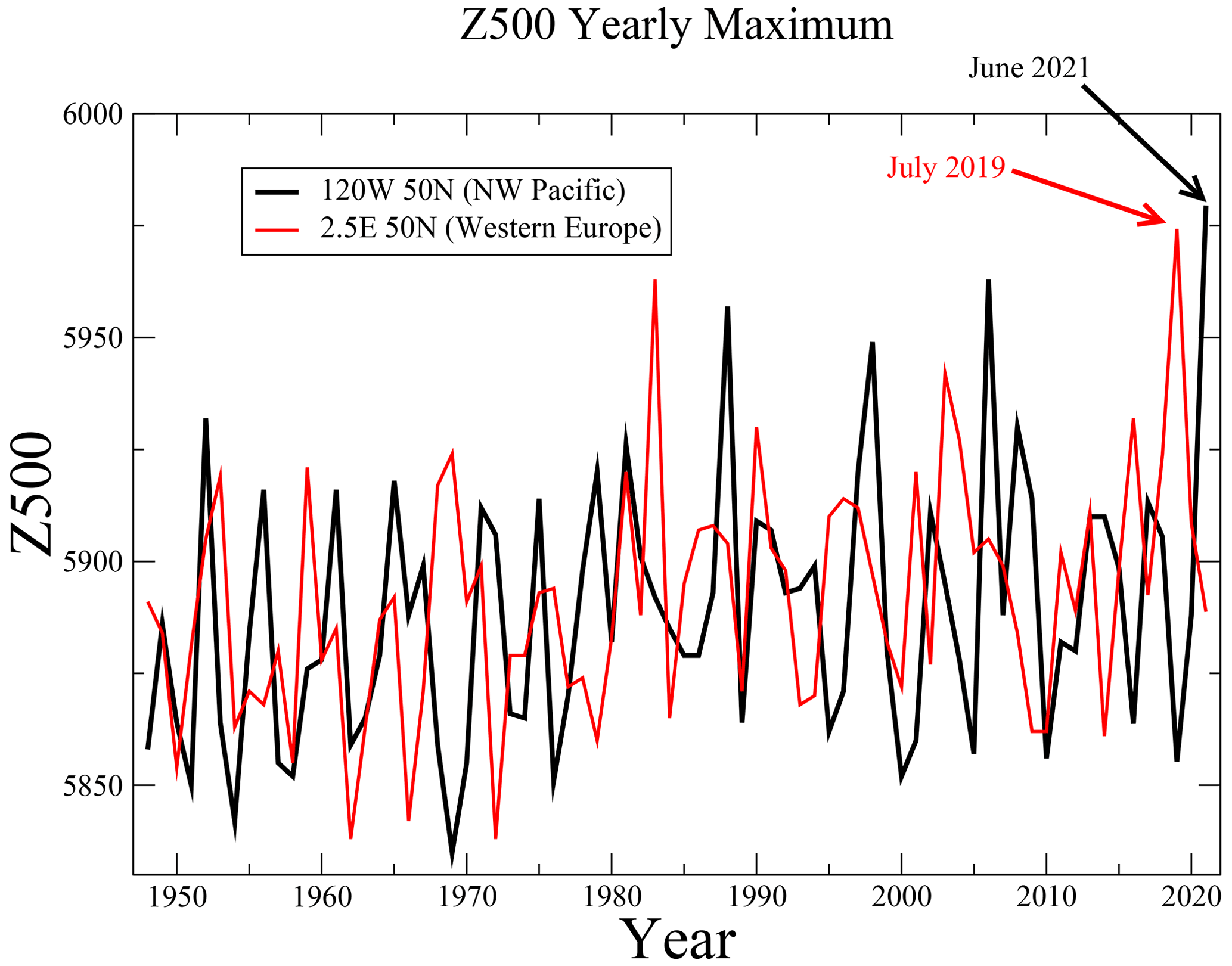
Figure 14 Annual maximum 500 hPa height (m) for two points at the same latitude on two continents. Black: Pacific Northwest (as above); red: western Europe (50^∘ N, 2.5^∘ E). Data source: NCEP initialised reanalysis (Kalnay et al., 1996).

Despite being a record, this extreme high-pressure system – a feature sometimes called a “heat dome” – is not that anomalous given the long-term trend in 500 hPa driven by thermal expansion (Christidis and Stott, 2015). Also, comparing recent heat waves in the Pacific Northwest to the extreme heat wave in western Europe in 2019 (Vautard et al., 2020), the geopotential height can be seen to reach similar anomalies and has a similar long-term trend (Fig. 14).

The circulation pattern itself also appears typical for hot summertime temperatures: using analogues of 500 hPa and a pattern correlation metric to compare fields, we find that about 1 % of June and July circulation patterns, defined as the 500 hPa geopotential height pattern within 35–65^∘ N, 160–110^∘ W, in previous years have an anomaly correlation larger than 0.8 with the 28 June pattern. This degree of correlation is typical among days with this type of blocking pattern during the months of June and July. Roughly one-third of June and July geopotential height fields have 1 % or fewer analogues with an anomaly correlation larger than 0.8. We also find that this fraction does not change when restricting the analogue search within three distinct time periods between 1948 and 2020. We conclude that the 28 June circulation is probably not exceptional, while temperatures associated with it were.

At the mesoscale, high solar irradiance during the longest days of the year and strong subsidence increased near-surface air temperatures during the event. As is typical for summer heat waves in the region (Brewer et al., 2012, 2013), a mesoscale thermal trough developed over western Oregon by 00:00 UTC on 28 June. This feature migrated northward, reaching the northern tip of Washington State by 00:00 UTC on 29 June. Further offshore, a small cut-off low travelled south-west to north-east around the synoptic-scale trough that made up the western arm of the omega block. The pressure gradients associated with the thermal trough and the cut-off low promoted moderate E–SE flow in the northern and eastern sectors of the feature and S–SW flow to the south. Near-surface winds with easterly components crossed the Cascade Range of Washington and Oregon and the southern Coast Mountains of British Columbia, where they were lighter but sufficient to displace cooler marine air. The difference in elevation on the western and eastern sides of the mountain ranges contributed to more adiabatic heating than cooling, which helped drive the warmest temperatures observed in the event along the foot of the western slope of these mountains, near or slightly above sea level. These dynamics are illustrated in Fig. 15. By 12:00 UTC on 29 June 2021, the south-western portion of the study area was under the influence of southerly to south-westerly near-surface flows that advected marine air and forced marked cooling. Unfortunately, winds associated with this transition intensified a wildfire that quickly consumed the town of Lytton, BC, where Canada's nationwide all-time high temperature was set just a day before.

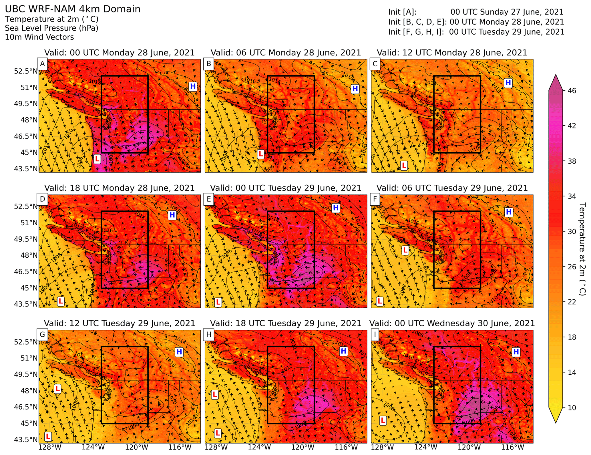
Figure 15 Regional simulation of sea level pressure, 2 m air temperature and 10 m wind velocity in the region containing the study area (black box) using the Weather Research and Forecasting (WRF; Skamarock et al., 2021) model forced by the North American Mesoscale Forecast System (NAM). Panels (a)–(i) show the evolution of the near-surface dynamics at a 6 h interval from 00:00 UTC on 28 June through 00:00 UTC on 30 June 2021. Of note is panel (e), which shows 17:00 local time on the day of peak temperature for Portland, Seattle and Vancouver. The H and L in the panels indicate high and low pressure.

There is no scientific consensus whether blocking events are made more severe or persistent because of Arctic amplification or other mechanisms (i.e. Tang et al., 2014; Barnes and Screen, 2015; Vavrus, 2018). We contend that Arctic sea ice was unlikely to have played a large role in this event largely due to the timing. In early summer, Arctic sea ice remains extensive but continues to melt, thus keeping near-surface temperatures near 0 ^∘C. This causes summer trends in near-surface temperatures over the Arctic Ocean to be smaller than for the midlatitudes. During the months prior to the event, the sea ice extent was below the 1981–2010 mean but was similar to values observed from 2011 to 2020 (Fetterer et al., 2017). Instead, Arctic amplification in summer is characterised by strong warming over high-latitude land areas (as can clearly be seen in Fig. 16), and this warming signal reaches into the upper troposphere. This enhanced warming is likely related to strong downward trends in early summer snow cover. There is evidence, from observations (Coumou et al., 2015; Chang et al., 2016), climate models (Harvey et al., 2020; Lehmann et al., 2014) and palaeo-proxies (Routson et al., 2019), that this enhanced warming over high latitudes leads to a weakening of the jet and storm tracks in summer. This weakening could favour more persistent weather conditions (Pfleiderer et al., 2019; Kornhuber and Tamarin-Brodsky, 2021). Regional-scale interactions between loss of snow cover and low soil moisture associated with earlier snowmelt and rapid springtime soil moisture drying may have had an enhanced warming impact into early summer in the Arctic. At mid-atmospheric levels there is some amplification remaining due to the winter season (Fig. 16), but at the jet level (∼250 hPa) the usual increase in the thermal gradient due to tropical upper-tropospheric warming is advected north by the Hadley circulation (Haarsma et al., 2013). The final effect on the jet stream is therefore a competition between factors enhancing and decreasing the temperature gradient.

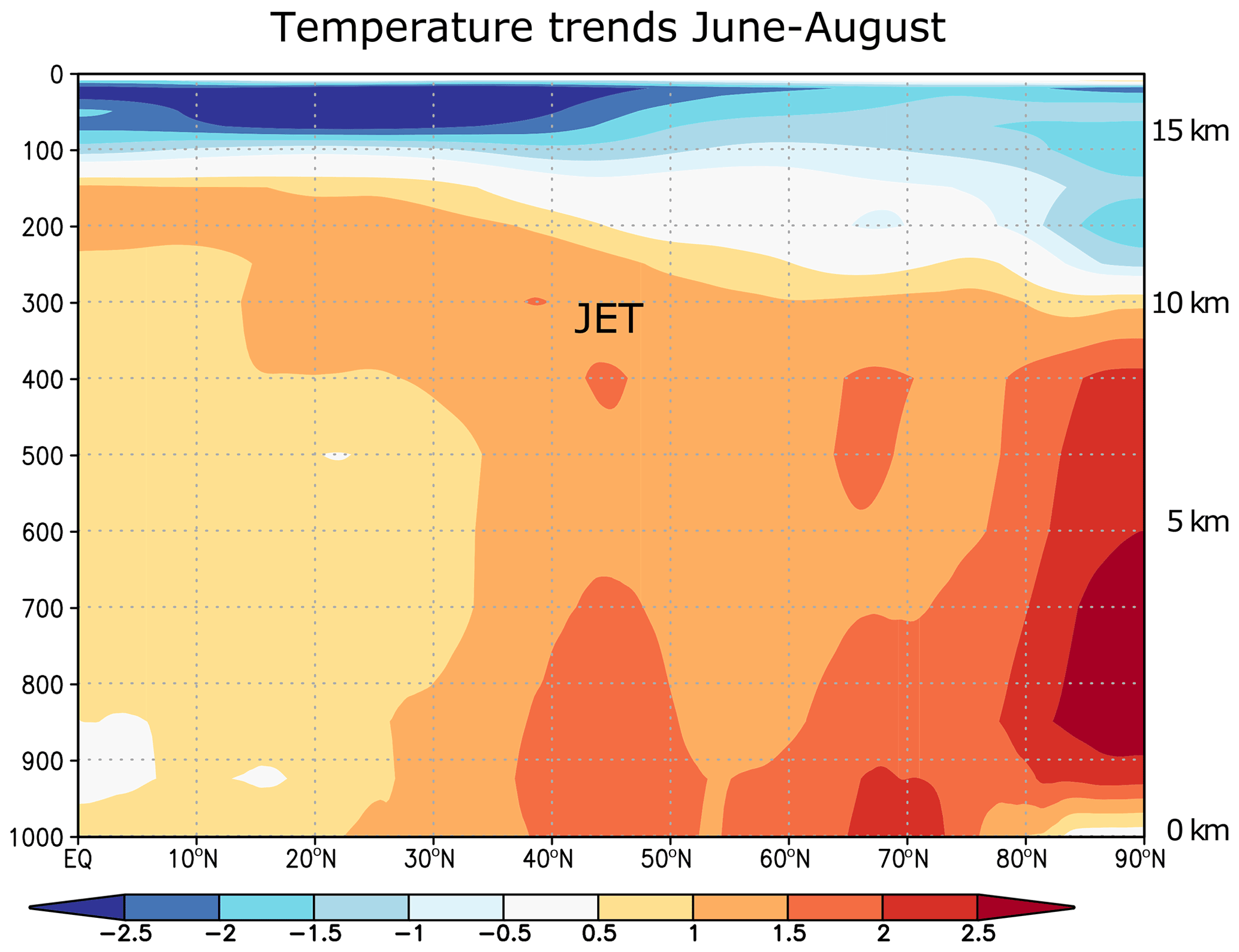
Figure 16 Zonal mean trends in temperature (degrees Celsius per degree global warming) as a function of pressure (hPa) in the ERA5 reanalysis 1979–2019 in the Northern Hemisphere.

6.3 Drought

An additional feature of the event is the very dry antecedent conditions that may have contributed to the observed extreme temperatures through reduced latent cooling from inhibited evapotranspiration. Low-soil-moisture conditions can lead to a strong amplification of temperature during heat waves, including nonlinear effects (Seneviratne et al., 2010; Mueller and Seneviratne, 2012; Hauser et al., 2016; Wehrli et al., 2019). In addition, low-spring-snow-level conditions can also further amplify this feedback (Hall et al., 2008). In this section we briefly explore whether precipitation anomalies and evapotranspiration measures could have played a role in the extreme heat via feedbacks related to soil moisture conditions.

Integrated Multi-satellitE Retrievals for the Global Precipitation Mission (IMERG) estimates of precipitation during the period from March through June 2021 indicate anomalously dry conditions from southern BC southward through California (Fig. 17). The relative precipitation anomaly ranges from close to zero over the Puget Sound area, including Seattle, to values of between −0.6 and −0.8, meaning that only 20 %–40 % of the average amount of precipitation fell in these locations, in western Oregon. Note that in the northern parts of the area affected by the heat wave, i.e. in the coastal mountains north of Vancouver Island, large positive precipitation anomalies occurred over the months prior to the event.

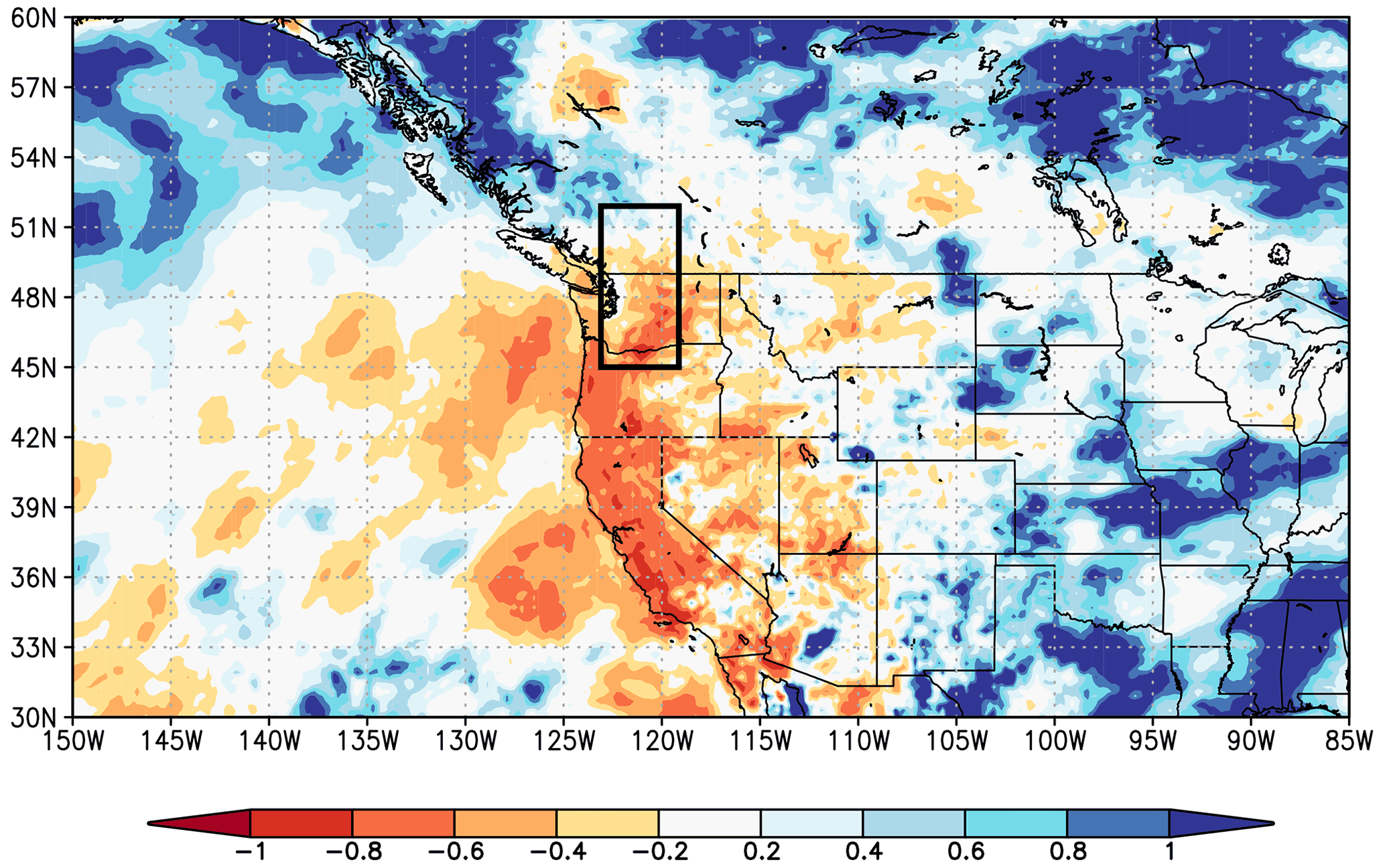
Figure 17 GPM/IMERG satellite estimates of relative precipitation anomalies in March–June 2021 relative to the whole record (2000–2020). The value −1 (dark red) denotes no precipitation, −0.5 (orange) 50 % less than normal and zero (light grey) normal precipitation. Origin: KNMI Climate Explorer.

The available moisture is also influenced by evapotranspiration, which depends strongly on temperature, radiation and available atmospheric moisture. Evaporation in the study area was below normal in the ERA5 reanalysis from March and became more negatively anomalous until May (not shown). During the event in late June, there was progressive soil desiccation, creating ideal conditions for strong negative evaporation anomalies. On the other hand, surface net radiation was high, especially before peak temperatures were reached (26–28 June). As a consequence, evaporation deficits during the heat build-up were rather slight compared to most days in May and the first half of June. Together with the extreme near-surface temperatures that suppressed surface heating due to an already hot surface, this resulted in only moderately positive surface sensible heat flux anomalies.

Satellite-based measurements of surface soil moisture based on microwave remote sensing from the European Space Agency (ESA) Climate Change Initiative (CCI) provided by the Copernicus service suggest that surface soil moisture was below normal in the region since the beginning of April and that the anomalous conditions persisted until June (https://dataviewer.geo.tuwien.ac.at/?state=88bf0c, last access: 6 July 2021), in agreement with the decreased precipitation and somewhat below-normal evapotranspiration in the ERA5 reanalysis.

6.4 Influence of modes of natural variability

The El  Niño–Southern Oscillation is the dominant source of interannual variability in the region through the Pacific North American teleconnection. The influence is typically greatest in late winter and spring and has less clear impacts during summer and fall. Because ENSO was neutral during the preceding months, and the impacts on TXx are minimal (r<0.1), we conclude that it had no influence on the occurrence of the heat wave.

The PDO can affect some aspects of North American summer weather, although again the connections to heat waves in this region are very weak. The strongly negative values of the PDO index, as they occurred in May, would slightly favour cooler conditions for this region. PDO thus also is unlikely to have played an important role in the event.

Altogether, external modes of variability appear to have played little to no role in the formation of the event.

7 Vulnerability and exposure

The Pacific Northwest region is not accustomed to very hot temperatures such as those experienced during the June 2021 heat wave. Heat waves are one of the deadliest natural hazards, resulting in high excess mortality through direct impacts of heat (e.g. heat stroke) and by exacerbating pre-existing medical conditions linked to respiratory and cardiovascular issues (Haines et al., 2006; Ebi et al., 2021). In addition to at least 815 excess heat-related deaths, there was a significant increase in emergency department visits (https://www.nytimes.com/interactive/2021/08/11/climate/deaths-pacific-northwest-heat-wave.html, last access: 22 August 2022; https://www.cbc.ca/news/canada/british-columbia/bc-heat-dome-sudden-deaths-570-1.6122316, last access: 22 August 2022). On 28 June 2021 alone, there were 1038 heat-related emergency department visits in the US Department of Health and Human Services region that includes Alaska, Idaho, Oregon and Washington, compared with 9 visits on the same date in 2019 (https://www.cdc.gov/mmwr/volumes/70/wr/mm7029e1.htm, last access: 22 August 2022). The mean daily number of heat-related-illness emergency department visits in the region for 25–30 June 2021 (424) was 69 times higher than during the same days in 2019 (6). Although this region covers about 4 % of the US population, it accounted for about 15 % of all heat-related-illness emergency department visits nationwide during June.

The June 2021 heat wave also affected critical infrastructure such as roads and rail and caused power outages and agricultural impacts and forced many businesses and schools to close (https://apnews.com/article/canada-heat-waves-environment-and-nature-cc9d346d495, last access: 6 July 2021; https://www.seattletimes.com/seattle-news/weather/pacific-northwests-record-smashing-heat-wave-primes-, last access: 6 July 2021). Rapid snowmelt in  BC caused water levels to rise, leading to evacuation orders north of Vancouver (https://globalnews.ca/news/7994540/flooding-record-breaking-heat-rapid-snow-melt-bc-video/, last access: 6 July 2021). Furthermore, in some places, wildfires, the risk of which has increased due to climate change in this region (Kirchmeier-Young et al., 2019), started and quickly spread, requiring entire towns to evacuate (https://www.washingtonpost.com/world/2021/07/01/lytton-canada-evacuated-wildfire-heatwave/, last access: 6 July 2021). The co-occurrence of such events may result in compound risks, for example when households are advised to shut windows to keep outdoor wildfire smoke from getting inside while simultaneously being threatened by high indoor temperatures when lacking air conditioning.

Timely warnings were issued throughout the region by the US National Weather Service, Environment and Climate Change Canada, and local governments. British Columbia has a Municipal Heat Response Planning summary review that gathers information on heat response plans throughout the province, including responses such as increasing access to cooling facilities and distribution of drinking water. In long-term strategies, changes to the built environment are emphasised (Lubik et al., 2017). Not all municipalities throughout the Pacific Northwest and BC have formalised heat response plans, and others have limited planning, thought to be due to low-heat-risk perceptions throughout the area, as well as a lack of local data for risk assessments (Lubik et al., 2017).

The extremely high temperatures that occurred in this heat episode meant that everyone was vulnerable to its effects if exposed for a long enough period of time. Although extreme heat affects everyone, some individuals are more vulnerable, including the elderly, young children, individuals with pre-existing medical conditions, socially isolated individuals, homeless people, individuals without air conditioning and (outdoor) workers (Singh et al., 2019). Seattle's King County contains the third-largest population of homeless people in the US, with the numbers increasing during the past decade (Stringfellow and Wagle, 2018). Governmental authorities opened cooling centres throughout Seattle, Portland and Vancouver during the June 2021 heat wave (https://durkan.seattle.gov/2021/06/city-of-seattle-opens-additional-cooling-centers-and-updated, last access: 6 July 2021; https://www.oregonlive.com/weather/2021/06/portland-cooling-centers-provide-relief-from-heat.html, last access: 6 July 2021; https://thebcarea.com/2021/06/26/cooling-stations-set-up-around-b-c-for-record-breaking-, last access: 6 July 2021). Further, electrolytes, food and water were distributed to homeless people (https://edition.cnn.com/2021/06/29/weather/northwest-heat-illness-emergency-room/index.html, last access: 6 July 2021).

The lack of air conditioning contributes to heat risk. The Pacific Northwest has lower access to air-conditioned homes and buildings compared to other regions in the US, with the Seattle metropolitan area being the least air-conditioned metropolitan area of the United States (<50 % air conditioning in residential areas) (US Census Bureau, 2019). Portland and Vancouver also have low percentages of air-conditioned households, 79 % and 39 %, respectively (BC Hydro, 2020; US Census Bureau, 2019). An increasing trend in air-conditioned homes is occurring in all three cities (BC Hydro, 2020; US Census Bureau, 2019).

8 Conclusions and recommendations

In this study, the influence of human-induced climate change on the intensity and probability of the Pacific Northwest heat wave of 2021 was investigated. We analysed how the annual maxima of daily maximum temperatures are changing with increasing global mean surface temperature, studying the area 45–52^∘ N, 119–123^∘ W, which includes the cities Vancouver, Seattle and Portland. Synthesising results from weather observations and model simulations, we conclude that the occurrence of a heat wave of the intensity experienced in the study area would have been virtually impossible without human-caused climate change. Whilst the extremity of this event made it challenging to robustly determine how rare it was in the current climate, this general result is not strongly tied to the exact return period. For this analysis, we defined the probability of the event as 1 in 1000 years in the current climate and found that the event would have been at least 150 times rarer without human-induced climate change. Also, this heat wave was found to be about 2 ^∘C (1.2 to 2.8 ^∘C) hotter due to human-induced climate change. Looking into the future to a world with 2 ^∘C of global warming, an event like this, estimated to occur only once every 1000 years in the current climate, would occur roughly every 5 to 10 years according to the best estimate, albeit with large uncertainties around it.

This record-breaking extreme event has been analysed under the assumption that it was simply a low-probability random event. A rudimentary calculation looking into the probability of a random event of similar extent and severity to occur anywhere over the Earth's land area gave an estimated chance on the order of 1 in 15 years, which at first impression makes a random event seem plausible, but this should be more thoroughly investigated.

The alternative is that nonlinear interactions and feedbacks occurred, which amplified the intensity of this extreme, placing it in a different population of heat wave events with different (and possibly unknown) statistics. We briefly considered dynamical and hydrological (drought) mechanisms and modes of natural variability that could have had an amplifying role. The conditions in the preceding months were dry but not extremely anomalous. The circulation itself was highly anomalous but not exceptional enough to explain the record-breaking heat alone; however, local topography and preceding dryness may have amplified the associated temperatures. Also, it cannot be excluded that dynamical mechanisms (Arctic amplification) at work influenced the persistence of blocking conditions.

Further research is planned to investigate whether these or other feedbacks were operating in this exceptional event, whether those feedbacks are related to human-induced climate change, and whether they increase the frequency beyond that expected for random events of such extreme temperatures. Also, further research is needed to overcome the known limitations of standard GEV analysis on annual maxima with short records and very extreme values.

Whether or not local or dynamical feedbacks are responsible for amplifying the extreme temperatures in this particular event, this study shows that the human-induced warming that has occurred since pre-industrial conditions does make extreme events like this possible in the current climate and study region, and many times more likely than in the pre-industrial era.

Adaptation measures therefore need to be much more ambitious and take account of the rising risk of heat waves around the world. Although this extreme heat event is still rare in today's climate, the analysis above shows that the frequency will increase with further warming. Deaths from extreme heat can be dramatically reduced with adequate preparedness action. A number of adaptation and risk management priorities are becoming clear: it is crucial that local governments and their emergency management partners establish heat action plans to ensure well-coordinated response actions during an extreme heat event – tailored to high-risk groups (Ebi, 2019). Heat wave early-warning systems also need to be improved, which includes tailoring messages to inform and motivate vulnerable groups, as well as providing tiered warnings that take into account that vulnerable groups may have lower thresholds for risk (Hess and Ebi, 2016). In other words, it is important to start to warn the most vulnerable as temperatures start to rise even though the general population is not yet acutely at risk. In cases where heat action plans and heat early-warning systems are already robust, it is important that they are reviewed and updated to capture the implications of rising risks – every 5 years or more often (Hess and Ebi, 2016). Further, heat wave early-warning systems should undergo stress tests to evaluate their robustness to temperature extremes beyond recent experience and to identify modifications to ensure continued effectiveness in a changing climate (Ebi et al., 2018).

Appendix A: Validation tables

Table A1 As Table 1 but showing all model validation results.

NA stands for “not available”.