the Creative Commons Attribution 4.0 License.
the Creative Commons Attribution 4.0 License.
 | 30 Aug 2022
Impact of an acceleration of ice sheet melting on monsoon systems
Alizée Chemison
Dimitri Defrance
Gilles Ramstein
Cyril Caminade
The study of past climates has demonstrated the occurrence of Heinrich events during which major ice discharges occurred at the polar ice sheet, leading to significant additional sea level rise. Heinrich events strongly influenced the oceanic circulation and global climate. However, standard climate change scenarios (Representative Concentration Pathways or RCPs) do not consider such potential rapid ice sheet collapse; RCPs only consider the dynamic evolution of greenhouse gas emissions. We carried out water-hosing simulations using the Institute Pierre Simon Laplace global Climate Model (IPSL-CM5A) to simulate a rapid melting of the Greenland and Antarctic ice sheets, equivalent to +1 and +3 m additional sea level rise (SLR). Freshwater inputs were added to the standard RCP8.5 emission scenario over the 21st century. The contribution to the SLR from Greenland or from Antarctic ice sheets has differentiated impacts. The freshwater input in the Antarctic is diluted by the circumpolar current, and its global impact is moderate. Conversely, a rapid melting of the ice sheet in the North Atlantic slows down the Atlantic Meridional Overturning Circulation. This slowdown leads to changes in winds, inter-hemispheric temperature and pressure gradients, resulting in a southward shift of the tropical rain belt over the Atlantic and eastern Pacific region. The American and African monsoons are strongly affected and shift to the south. Changes in the North American monsoon occur later, while changes in the South American monsoon start earlier. The North African monsoon is drier during boreal summer, while the southern African monsoon intensifies during austral summer. Simulated changes were not significant for the Asian and Australian monsoons.
- Article
(18460 KB) - Full-text XML
- BibTeX
- EndNote


Monsoons influence tropical regions without a perennial rain regime, providing the vast majority of rainfall in one season (Wang and Ding, 2006). Consequently, monsoons have a significant impact on two-thirds of the world's population (Wang and Ding, 2006; Moon and Ha, 2020). Tropical monsoons have large inter-annual to multi-decadal variability that modulates drought, flooding and other climatic extremes that have strong impacts on human societies, agriculture and economy. Monsoons are related to atmospheric moisture content, land–sea temperature contrast (Li and Yanai, 1996; Sutton et al., 2007; Zhou and Zou, 2010; Fasullo, 2012), thermodynamic and dynamic features (Kitoh et al., 2013; Endo and Kitoh, 2014), land cover and use (Timbal and Arblaster, 2006), atmospheric aerosol loadings (Lau et al., 2008), and the vegetation physiological effect of rising atmospheric CO2 (Cui et al., 2020). Climate change is expected to significantly alter monsoon systems (Zhisheng et al., 2015). Studying the future evolution of monsoons is essential to guide adaptation measures. Climate change impact on tropical monsoons has been extensively studied using coupled global climate models (GCMs) that provide predictions of future climate under various greenhouse gas (GHG) emission scenarios. The Coupled Model Intercomparison Project 5 (CMIP5) aimed to coordinate climate simulations produced by different international research groups. CMIP5 used the Representative Concentration Pathway (RCP) scenarios (Meehl et al., 2000), which are GHG emission pathways in CO2 equivalent, corresponding to different radiative forcing scenarios at the end of the 21st century (Moss et al., 2010; Taylor et al., 2012). From these scenarios, it has been shown that monsoons are significantly affected by climate change (Wang et al., 2021).
It is difficult to estimate the evolution of the global monsoon in the short term (2020–2040) because the uncertainty and internal variability across GCMs are more important than the signal itself (Lee et al., 2021). Nevertheless, precipitation is expected to increase by 1 % to 3 % per 1 ∘C increase during the midterm (2041–2060) and long term (2081–2100); see Lee et al. (2021). The global monsoon area, total precipitation and precipitation intensity are simulated to increase by most CMIP5 models at the end of the 21st century (Hsu et al., 2013; Kitoh et al., 2013). These increases are linked to an increase in evaporation and therefore to an increase in atmospheric moisture flow, but also to increased temperature contrast between the continents and the oceans. Continents are warming up faster than the oceans in the context of global warming. Moreover, Lee and Wang (2014) show a zonal asymmetry between the eastern monsoons, with increased precipitation, and the western monsoons, with decreased precipitation. They also show an asymmetry between the Northern and Southern Hemisphere. The Northern Hemisphere will receive more rainfall in the future, while the Southern Hemisphere will receive less. In the Northern Hemisphere the monsoon period lasts longer with an earlier start and later cessation date (Lee and Wang, 2014). Extreme precipitation events and days of drought conditions are also simulated to increase in future (Cavazos et al., 2008; Shongwe et al., 2011).
At regional scale, monsoons are differently affected by climate change. CMIP3 and CMIP5 models show a rainfall increase across the Asian monsoons (Turner and Annamalai, 2012; Li et al., 2015). These changes are considered with medium confidence in the latest IPCC report (Ranasinghe et al., 2021). The East Asian monsoon (EAS) and the southern Asian monsoon (Indian monsoon) are intensifying with increasing mean and extreme rainfall (Jiang et al., 2012). A longer season for EAS was highlighted by Suhaila et al. (2010).
For the Maritime Continent region (between Asia and Australia) and Australia, the multi-model agreement for future rainfall changes is low (Christensen et al., 2013; Ranasinghe et al., 2021), and current state-of-the-art GCMs are not suited to capture the fine-scale climatic processes occurring in this region (Turner and Annamalai, 2012). Jourdain et al. (2013) show an increase in Australian rainfall using RCP8.5 at the end of the 21st century.
For the Americas, two monsoon systems are commonly identified (Christensen et al., 2013): the North American monsoon system (NAMS) and the South American monsoon system (SAMS). For the NAMS, a decrease in precipitation is simulated over the 21st century, although significant differences are shown across GCMs (Wang et al., 2021). However, there is a robust increase in temperature as well as the number of dry days and extreme events simulated over this region at the end of the 21st century (Duffy and Tebaldi, 2012). A shift in the NAMS is also simulated, with a decrease in rainfall at the beginning of the season and an increase towards the end (Cook and Seager, 2013). For the SAMS, there is a seasonal amplification with an earlier start and later cessation date (Jones and Carvalho, 2013).
Over eastern Africa, two rainy seasons occur: the so-called short rains from October to December and long rains from March to May. A significant increase in future rainfall during the long rainy season is usually simulated over East Africa (Ongoma et al., 2018), although important biases exist in this region (Yang et al., 2015). For the West African monsoon, there are large rainfall differences simulated across GCMs (Biasutti et al., 2009; Monerie et al., 2020). However, simulated trends for CMIP3 and CMIP5 are similar, with drying simulated during spring and an increase in precipitation simulated in summer (Biasutti and Sobel, 2009; Biasutti, 2013; Christensen et al., 2013; Seth et al., 2013). Dunning et al. (2018) show a later onset of the monsoon season with a northward shift of the rain belt between August and December. The study of Biasutti and Sobel (2009), based on CMIP3 models, projects a shorter rainy season with a late start of the semi-arid African Sahel. A delayed start of the rainy season has also been demonstrated by Song et al. (2021) using observed precipitation data. An extension of the dry season is simulated over the southern part of Africa (Mariotti et al., 2014).
The study of paleoclimatology with GCMs has shown the ability of models to simulate strong changes in precipitation at longer timescales. For example, the simulation of the green Sahara during the middle Holocene has always been challenging, with climate models usually underestimating the northward extension of the African monsoon. Nevertheless, the inclusion of new processes and boundary conditions including lakes (Krinner et al., 2012) or aerosols (Thompson et al., 2019) allowed simulations to reproduce the greening of the Sahara during the early to mid-Holocene (Krinner et al., 2012). Climate observations and future climate scenarios both indicate that global warming is occurring and the warming is more pronounced at high latitudes. This warming at the poles leads to an increase in ice sheet melting (Peterson et al., 2006). This melting releases a significant volume of fresh water, which contributes to additional sea level rise (SLR) (Rignot et al., 2011).
Melting is a non-linear process due to positive feedbacks associated with temperature increase (Fettweis et al., 2013). The melting of the ice sheet decreases surface albedo and consequently the surface absorbs more solar energy, leading to additional ice sheet melting. In addition, rising temperature can lead to increased liquid with respect to solid precipitation at high latitudes, which can increase the ice sheet mass loss. This mechanism occurs for the Greenland Ice Sheet (Fettweis et al., 2013), unlike Antarctica, where an increase in solid precipitation makes the mass balance more complicated to predict (Rignot et al., 2011). Finally, a fraction of mass loss is in relation to the glacier dynamics (Rignot et al., 2011; Fettweis et al., 2013). Observations suggest important processes responsible for glacier front destabilization that are not included in current state-of-the-art dynamical ice sheet models, such as the role of ice discharge in the total Greenland Ice Sheet mass balance (Gillet-Chaulet et al., 2012). Such destabilization could lead to an iceberg break-up, which in some ways might be similar to past Heinrich events (Broecker et al., 1992). It is noteworthy that deglaciation occurred over several thousand years when CO2 concentration only varied from 180 ppm (glacial period) to 280 ppm (interglacial period). Recent historical CO2 emissions ranged from 280 to 415 ppm, and they might reach 500 ppm or more by the end of the 21st century. In addition, the last deglaciation occurring during the first half of the Holocene was strongly non-linear, with an accelerated phase of melting (Mimura, 2013). Therefore, it is important to estimate the impact of such accelerated phases associated with Greenland and Antarctica melting (Hemming, 2004). The SLR predicted at the end of the 21st century by the IPCC fifth Assessment Report (AR5) ranges between 0.52 and 0.98 m (Church et al., 2013). Nevertheless, non-linear climatic processes may occur; for instance, DeConto and Pollard (2016) have shown that a rapid ice sheet destabilization could lead to an additional SLR exceeding 1 m.
GCMs are often not fully coupled with ice sheet models. Even if some GCMs include melting ice (Church et al., 2013), studies have shown that the melting predicted by these models is underestimated (Rignot et al., 2011; Gillet-Chaulet et al., 2012). Estimates of additional SLR are not directly available from GCMs outputs. Ice sheet models or regional models forced by temperature and rainfall simulated by GCMs are used to estimate additional SLR offline (Fettweis et al., 2013). However, the addition of fresh water due to the melting of the ice sheet at high latitudes is having a global impact on the climate (Mimura, 2013).
A major release of fresh water, linked to the tipping point of the ice sheet, would not be without consequences. In Greenland, the inputs of fresh water slow down the Atlantic Meridional Overturning Circulation (AMOC) (Bakker et al., 2016). A release of fresh water in the North Atlantic leads to a cooling of the Northern Hemisphere and a southward shift of the Intertropical Convergence Zone (ITCZ) in the Atlantic (Schiller et al., 1997; Vellinga and Wood, 2002; Jackson et al., 2015). This finding is consistent at different timescales: for paleo-modelling studies (Kageyama et al., 2013; Marzin et al., 2013a), for pre-industrial historical simulations (Vellinga and Wood, 2002; Stouffer et al., 2006) or for future climate simulations considering an increase in GHG emissions (Vellinga and Wood, 2008; Liu et al., 2020). A slowdown of the AMOC will also affect the Pacific Meridional Overturning Circulation (PMOC) with potential changes in associated temperature and precipitation patterns at global scale (Liu and Hu, 2015). This is clearly demonstrated in paleoclimatology during Heinrich events; it is possible to find proxies for induced changes in temperature and precipitation in many places on Earth (Clement and Peterson, 2008). Simulations of such a rapid melting have impacts on the Asian monsoon (Marzin et al., 2013b) and the African monsoon (Mulitza et al., 2008; Marzin et al., 2013a), and they might induce changes in European and American temperature and precipitation (Jackson et al., 2015). These feedbacks and the magnitude of temperature and precipitation changes outside the North Atlantic region depend on the mean simulated climate (Swingedouw et al., 2009b). Although GCMs have biases, the consequences of an influx of fresh water into the North Atlantic, a cooling of the North Atlantic and a southward shift of tropical precipitation have been shown in simulations conducted with different GCMs (Stouffer et al., 2006; Swingedouw et al., 2013). The melting of Antarctica can moderate the simulated rise in temperature in the Southern Hemisphere (Swingedouw et al., 2008). Competition between the deep waters formed in the North Atlantic (NA) and the Southern Ocean (SO) leads to a process called the bipolar oceanic seesaw (Stocker, 1998). Swingedouw et al. (2009a) show that the release of fresh water in the Southern Hemisphere, linked to the melting of the Antarctic, can impact NA Deep Water (NADW). This effect occurs because of three processes: the deep-water adjustment which strengthens the NADW cell, the SO salinity anomaly which weakens the NADW cell and the increase in wind stress in the Southern Hemisphere which strengthens the NADW cell. These processes act on different timescales ranging from a few to 30 years (Swingedouw et al., 2009a).
Previous studies have shown that freshwater release from melting ice sheets can have a major impact on climate (Defrance et al., 2017, 2020). However, the response of global and regional monsoons to such rapid ice melting has not been investigated in great detail. The main objective of this study is to determine the impact of melting ice sheets on global monsoon but also on each regional monsoon using detailed analysis of mechanisms at play. In this study we highlight potential changes in rainfall seasonality and intensity using Hovmöller diagrams. We also investigate mechanisms at play at the ocean–atmosphere–cryosphere interface and assess the relationship between rainfall changes and moist static energy using the IPSL-CM5A-LR model.
To determine the impact of a significant release of fresh water at high and low latitudes on tropical monsoons, we used a simulation framework developed by Defrance et al. (2017). A release of fresh water is simulated in the North Atlantic (offshore Antarctica) to simulate a partial melting of the Greenland (West Antarctica) Ice Sheet. This freshwater release is added to the standard RCP8.5 scenario to simulate a break-up of the ice sheet using the Institute Pierre Simon Laplace Climate Model version 5A (IPSL-CM5A).
This study aims to understand the impact of a rapid ice sheet melting on monsoons and the physical mechanisms at play. First, we focus on the impact of ice sheet melting on oceanic and atmospheric circulation (Sect. 3.1 and 3.2, respectively). In a second step, we will study more detailed impacts of such melting on monsoons, first globally and then regionally (Sect. 3.3 and 3.4, respectively). Finally, we will discuss these results and provide final recommendations (Sect. 4).
2.1 Climate model
All experiments were conducted with the IPSL-CM5A model at low spatial resolution (IPSL-CM5A-LR, 3.75∘ in longitude and 1.875∘ in latitude) using the r1i1p1 simulation as described by Dufresne et al. (2013). IPSL-CM5A is one of the global climate models used for CMIP5 (Taylor et al., 2012) that feeds into the IPCC 5th assessment report. This model is a atmosphere–ocean global climate model (AOGCM). This GCM includes an atmosphere–land surface model coupled to an ocean–sea ice model. This model is made up of physical and biogeochemistry models (Dufresne et al., 2013). The dynamical atmospheric model is LMDz (Laboratoire de Météorologie Dynamique zoom) version 5A with 39 vertical levels, 15 of which are below 20 km (Hourdin et al., 2013). The ORCHIDEE (ORganizing Carbon and Hydrology In Dynamic EcosystEms) land surface model is included in IPSL-CM5A-LR (Krinner et al., 2005). NEMOv3.2 (for Nucleus for European Modelling of Ocean) is the ocean model included in IPSL-CM5A (Madec et al., 2017). The resolution is about 2∘ (with a meridional increased resolution of 0.5∘ near the Equator) with 31 vertical levels for the ocean (Dufresne et al., 2013). NEMOv3.2 includes the simulation of ocean dynamics with OPA (Océan PArallélisé), biogeochemistry processes with PISCES (Pelagic Interaction Scheme for Carbon and Ecosystem Studies) (Aumont and Bopp, 2006) and sea ice processes with LIM2 (Louvain-la-Neuve Sea Ice Model, Version 2) (Fichefet and Maqueda, 1997). The OAsis (Ocean Atmosphere Sea Ice Soil) coupler allows the synchronization of all models and the exchange of energy and moisture fluxes between the different sub-climatic systems (Valcke, 2013). The biogeochemistry models are INCA (The INteraction with Chemistry and Aerosol) for tropospheric chemistry and aerosols (Hauglustaine et al., 2004) and the REPROBUS (Reactive Processes Ruling the Ozone Budget in the Stratosphere) module for stratospheric chemistry (Lefevre et al., 1994). The prescribed variables are CO2 and other greenhouse gas emissions based on RCP scenarios (Moss et al., 2010), land use (Hurtt et al., 2011), solar irradiance (Lean et al., 2005), and volcanic aerosols (Dufresne et al., 2013).
2.2 Experimental design
The experimental design used in this study (Chemison et al., 2022) is based on Defrance et al. (2017). The RCP8.5 scenario (Moss et al., 2010) is used as our reference simulation. RCP8.5 is a worst-case scenario assuming the continuation of recent trends without mitigation during the 21st century and leading to an atmospheric radiative imbalance of 8.5 W m−2 by 2100 (Moss et al., 2010). To simulate the ice sheet melting, two sets of simulations were used. The first one corresponds to a partial melting of the Greenland Ice Sheet (GrIS scenarios) and the second one to a melting of the West Antarctic Ice Sheet (WAIS scenarios). Freshwater fluxes (FWFs) of 0.22 and 0.68 Sv (where 1 Sv = 106 m3 s−1) for the GrIS scenarios and 0.68 Sv for the WAIS scenario were introduced from 2020 to 2070 using the common RCP8.5 radiative forcing scenario, leading to +1 and +3 m additional SLR, respectively. These simulations are hereafter referred as to GrIS1m, GrIS3m and WAIS3m. The annual rate of freshwater release (0.68 or 0.22 Sv depending on the simulation) is constant over 2020–2070. For the GrIS scenarios, the fresh water is added in the North Atlantic (45–65∘ N, 45∘ W–5∘ E) where deep water is formed. For WAIS3m, fresh water is added into the western Antarctic Ocean off the coasts of southern America (Defrance et al., 2020). The choice to introduce large amounts of fresh water aims to magnify potential impacts of rapid ice sheet melting on monsoon systems, despite known low sensitivity of current climate models to the amount of freshwater release (Swingedouw et al., 2013; Hansen et al., 2016).
We compare a mid-century period (2041–2070) during freshwater release with the historical period (1976–2005) for RCP8.5, GrIS and WAIS scenarios. For all experiments, only one simulation was used (see Appendix A for further details about model internal variability). To quantify the potential impact of melting ice sheet on ocean circulation, we study the evolution of the AMOC, which is derived from the maximum annual mean stream function at 30∘ N based on the criterion by Cheng et al. (2013).
2.3 The monsoon domains
Monsoon areas are defined based on the criterion by Lee and Wang (2014). A monsoon area is characterized by an annual difference in precipitation between local summer and winter exceeding a threshold of 2.5 mm d−1, and the summer precipitation must exceed 55 % of the annual total. To compare observed and simulated monsoon areas, observed rainfall data are based on the Global Precipitation Climatology Project (GPCP, monthly V2.3) available from the NOAA PSL, Boulder, Colorado, USA (Adler et al., 2018). These data were averaged between 1979 and 2005 and compared with the historical simulation from 1976 to 2005.
Table 1List of regions and the associated monsoon period. Only land grid points are used in the analysis. See Fig. 1 for the graphical representation of regions.
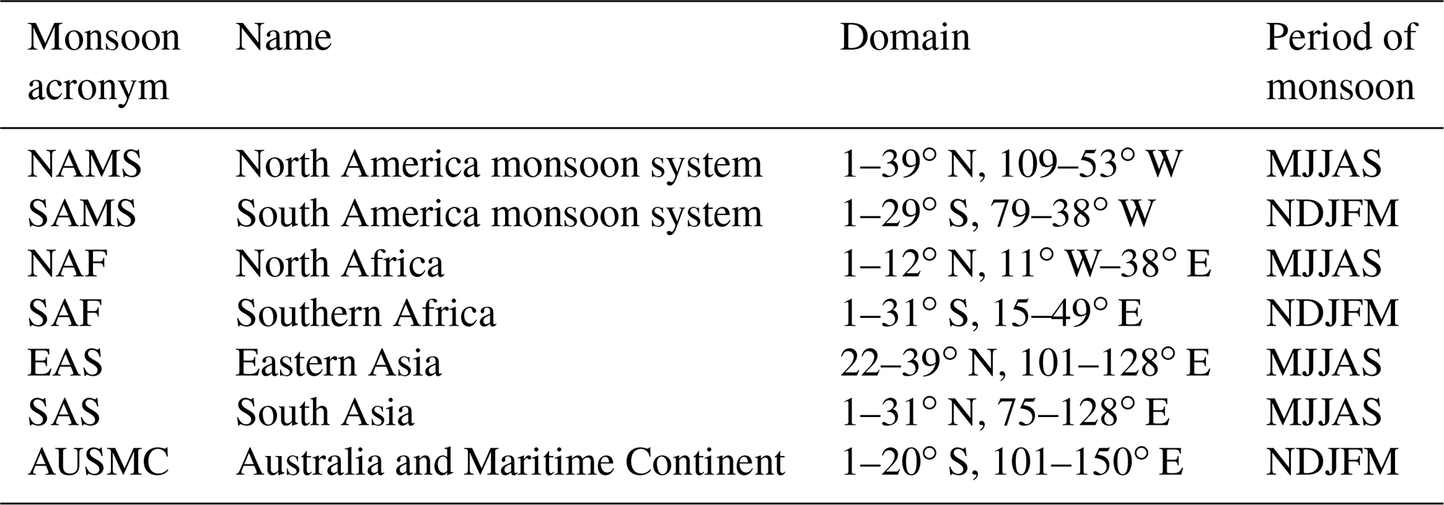

Figure 1Regions used in this study. See Table 1 and the Methods section for more details.
Each regional monsoon was defined following the fifth IPCC report naming convention (Fig. 14.3 in Christensen et al., 2013): the North America monsoon system (NAMS), South America monsoon system (SAMS), North Africa (NAF), southern Africa (SAF), eastern Asia (EAS), South Asia (SAS), and Australia and the Maritime Continent (AUSMC); see Table 1 and Fig. 1. The Equator separates the Northern Hemisphere monsoons, whose summer wet season lasts from May until September (MJJAS), and the Southern Hemisphere monsoons during which the summer period lasts from November to March (NDJFM) following Wang and Ding (2008), Wang et al. (2011), and Lee and Wang (2014).
Monsoon areas consist of any land grid point corresponding, in at least one of the simulations, to the aforementioned criterion (Lee and Wang, 2014). Thus, the selected monsoon areas include monsoon regions for historical and scenario simulations (RCP8.5, GrIS1m, GrIS3m, WAIS3m). All land grid points per monsoon region were retained to derive spatial averages, except for the AUSMC box for which one outlier (southernmost point) was removed. Only land data were considered.
To better understand simulated precipitation changes, we calculated moist static energy (MSE; in J kg−1) as follows:
cp (J kg−1 K−1) is the specific heat at constant pressure, T (K) is the layer temperature, g (m s−2) is the gravity constant, Z (m) is the geopotential height, L (m2 s−2) is the latent heat of evaporation and q (kg kg−1) is the specific humidity.
Hovmöller diagrams were derived for each land monsoon region. Rainfall was averaged longitudinally. They represent the average monthly precipitation over our 30-year study period. Then, the difference between the future period (2041–2070) and the historical period 1976–2005) was calculated. The statistical significance of this difference was evaluated using the Wilcoxon–Mann–Whitney test for p values greater than 0.05 (Seneviratne et al., 2013).
For each land monsoon area, ΔMSE, the difference between the MSE at 200 and 850 hPa, was calculated following Seth et al. (2013).
Then, the ΔMSE difference between the future and historical period is calculated for each future simulation and for each region (ΔMSE anomaly hereafter). The ΔMSE anomaly was averaged longitudinally and monthly and overlaid on the Hovmöller precipitation diagrams.
Hovmöller diagrams are shown for NAMS, SAMS, NAF, SAF and SAS. Diagrams for AUSMC and EAS are presented in Appendix C. It is noteworthy that changes for AUSMC and EAS are mostly non-significant, and too few land pixels were available for the AUSMC region.
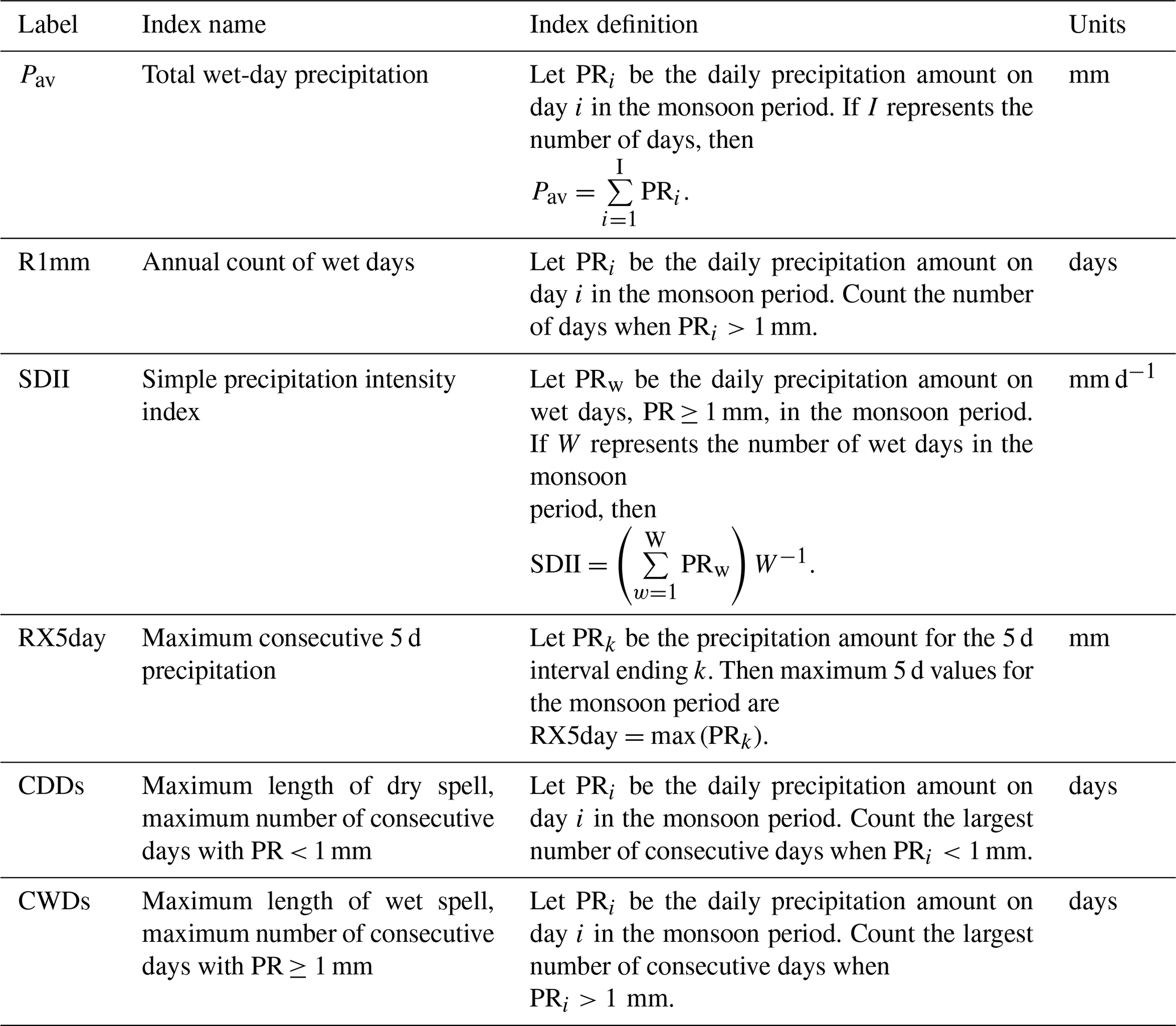
Table 2Definition and description of land monsoon indices during the monsoon period used in this study.
2.4 Characterization of monsoons
Six indices, defined by the Expert Team on Climate Change Detection and Indices (ETCCDI), were used to determine changes in daily rainfall extremes and statistics per land monsoon region (Sillmann et al., 2013): the total precipitation (Pav), the number of rainy days (R1mm), simple precipitation daily intensity index (SDII), seasonal maximum 5 d precipitation total (RX5day), seasonal maximum consecutive dry days (CDDs) and seasonal maximum consecutive wet days (CWDs). The indices are calculated annually for the May to September period over the Northern Hemisphere and for the November to March period for the Southern Hemisphere. Calculation details for each index are provided in Table 2.
These indicators can be used to study the impacts of changes in rainfall. They can then be used for population adaptation. In order to have the most accurate indices possible, we have chosen to apply a bias correction to rainfall by the cumulative distribution function transform (CDF-t) method that was developed by Michelangeli et al. (2009). For this purpose, by a mathematical transfer function (Vrac and Friederichs, 2015), the CDF of the precipitation variable simulated by the IPSL-CM5A-LR is matched to the CDF of the observed precipitation, here the watch forcing data by making use of the ERA-Interim (WFDEI) (Famien et al., 2018). This dataset is derived from the ERA-Interim (Dee et al., 2011) reanalyses. It extends from 1 January 1979 to 31 December 2013 and has a horizontal resolution of . Thus, before being able to set up the CDF matching, the precipitation data from the GCM were spatially interpolated on the same grid. Due to the importance of seasonality for the monsoons, the CDF-t method is applied monthly. This method preserves the long-term trends, but moments or quantiles are not conserved (Vrac and Friederichs, 2015).

Figure 2Stream function difference between future scenarios (2041–2070) and historical simulation (1976–2005). The future scenarios are (a) RCP8.5, (b) WAIS3m, (c) GrIS1m and (d) GrIS3m.
The validation of these indicators for our simulations is presented in Appendix C (Fig. C2) by comparing the inter-annual variability of each index for each monsoon between the historical simulation and the EartH2Observe, WFDEI and ERA-Interim data Merged and Bias-corrected data for ISIMIP (EWEMBI) (Lange, 2016). To study the impact of each simulation on these monsoon indices, the difference in inter-annual variability for each simulation between the period 2041–2070 and the historical simulation 1976–2005 is then calculated as the difference between a year and the historical mean divided by the historical mean and converted to a percentage:
These results are presented in the form of box-and-whisker plots for each region and each simulation.
3.1 Ocean dynamics
The most direct impact of the addition of fresh water, resulting from an ice melting, occurs in the ocean. Future changes for the RCP8.5 simulation correspond to a −4 Sv decrease of the stream function between 500 and 2500 m depth in the North Atlantic (Fig. 2a). This difference is slightly reduced for the WAIS3m scenario (Fig. 2b), denoting a moderate impact of Antarctica ice melting on the North Atlantic Ocean circulation. This moderate impact may be related to the presence of the circumpolar current around the Antarctica continent, which tends to dilute the FWF disturbance. Conversely, the addition of FWF in the North Atlantic associated with the melting of the Greenland Ice Sheet strongly amplifies the simulated decrease in stream function (about −6 Sv between 500 and 2500 m). The larger the amount of fresh water added, the greater the decrease in simulated oceanic stream function (Fig. 2c and d). The addition of fresh water in the North Atlantic changes the water density, resulting in changes in oceanic currents. The seasonal signal is weak, although there are slightly stronger differences simulated in boreal summer with respect to winter for the GrIS scenarios (see Figs. B1 and B2).
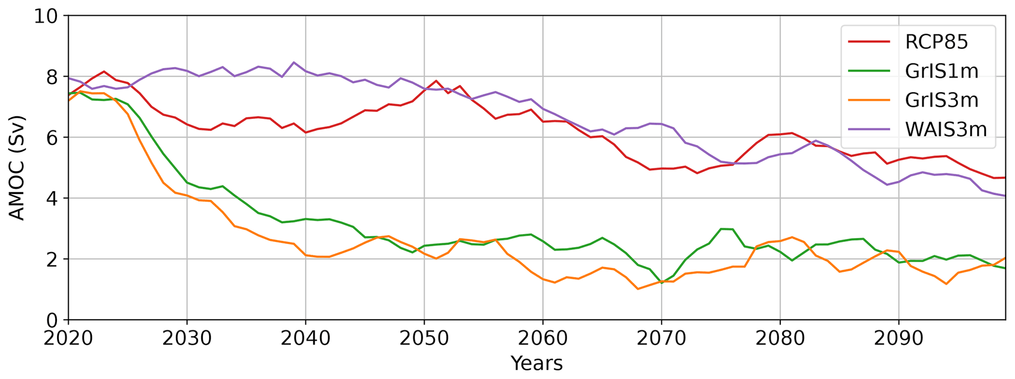
Figure 3Simulated AMOC between 2020 and 2099 for different scenarios: RCP8.5 in red, GrIS1m in green, GrIS3m in orange and WAIS3m in purple. The AMOC index is derived from the maximum annual mean stream function at 30∘ N from Cheng et al. (2013).
These results are consistent with the simulated evolution of the AMOC during the 21st century (Fig. 3). In 2020, before the simulated release of fresh water, all simulations are extremely similar. Simulated AMOC ranges between 7 and 8 Sv, and small differences across simulations might be related to internal model variability (Fig. 3). Between 2025 and 2050, the AMOC simulated for the RCP8.5 scenario decreases to 6 Sv and then increases to 8 Sv, while the AMOC for the WAIS3m scenario remains relatively constant. After 2050, the AMOC slowly decreases to 4 Sv for WAIS3m and 5 Sv for RCP8.5. The AMOC simulated for the scenarios with the melting of the Greenland Ice Sheet, GrIS1m and GrIS3m, shows larger changes. For GrIS1m and GrIS3m, the AMOC decreases to 4 Sv between 2025 and 2030, then to 2 Sv between 2040 and 2050, with a 1 Sv minimum reached between 2060 and 2070. From 2070 onwards, freshwater release stops in our experiments; the AMOC simulated by GrIS1m and GrIS3m then stabilizes and oscillates at values of about 2 Sv. The release of fresh water in Antarctica (WAIS3m) initially buffers the simulated slowdown of the AMOC in the RCP8.5 experiment (Fig. 3). Freshwater input in the North Atlantic breaks down the AMOC, with an almost complete collapse simulated by 2060–2070 (Fig. 3). The amount of released fresh water in the North Atlantic has a limited impact on AMOC changes, as values for the GrIS1m and GrIS3m scenarios are relatively similar for the 21st century (Fig. 3).

Figure 4Difference between future scenarios (2041–2070) and historical simulation (1976–2005) for the boreal summer season (MJJAS). The left column depicts the surface temperature difference (a, c, e, g), and the right column shows the difference in rainfall (shading), SLP (black contours, dashed lines for negative values) and wind at 850 hPa (vectors) (b, d, f, h). The future scenarios are (a, b) RCP85, (c, d) WAIS3m, (e, f) GrIS1m and (g, h) GrIS3m.
3.2 Atmosphere dynamics
Differences between future scenarios and the historical period are shown for several atmospheric variables (temperature, rainfall, sea level pressure and winds at 850 hPa) during boreal summer in Fig. 4 and austral summer in Fig. 5. A large increase in temperature is shown at global scale for the RCP8.5 scenario, with simulated temperature differences of about 10 ∘C at the North Pole during boreal winter (Fig. 5a). This high-latitude increase in temperature is slightly amplified in the WAIS3m scenario (Fig. 5c). Conversely, the effect of the RCP8.5 radiative forcing on temperature is strongly buffered by the melting of the Greenland Ice Sheet (GrIS1m and GrIS3m) (Figs. 4e–g and 5e–g). Simulated temperature increases for GrIS1m (Figs. 4e and 5e) and GrIS3m (Figs. 4g and 5g) are much smaller all year round. The fresh water released into the North Atlantic cools down this region; this local cooling extends to the western part of the North Atlantic Ocean for GrIS3m (Figs. 4g and 5g). The induced cooling of the North Atlantic is more pronounced during boreal winter (Fig. 5e–g). For the WAIS3m simulation, the cooling due to the melting of western Antarctica is shown during austral summer (Fig. 5c) and is greatly amplified during austral winter (Fig. 4c). WAIS3m shows a regional cooling along the Antarctica coast, which is linked to the circumpolar current (Figs. 4c and 5c).
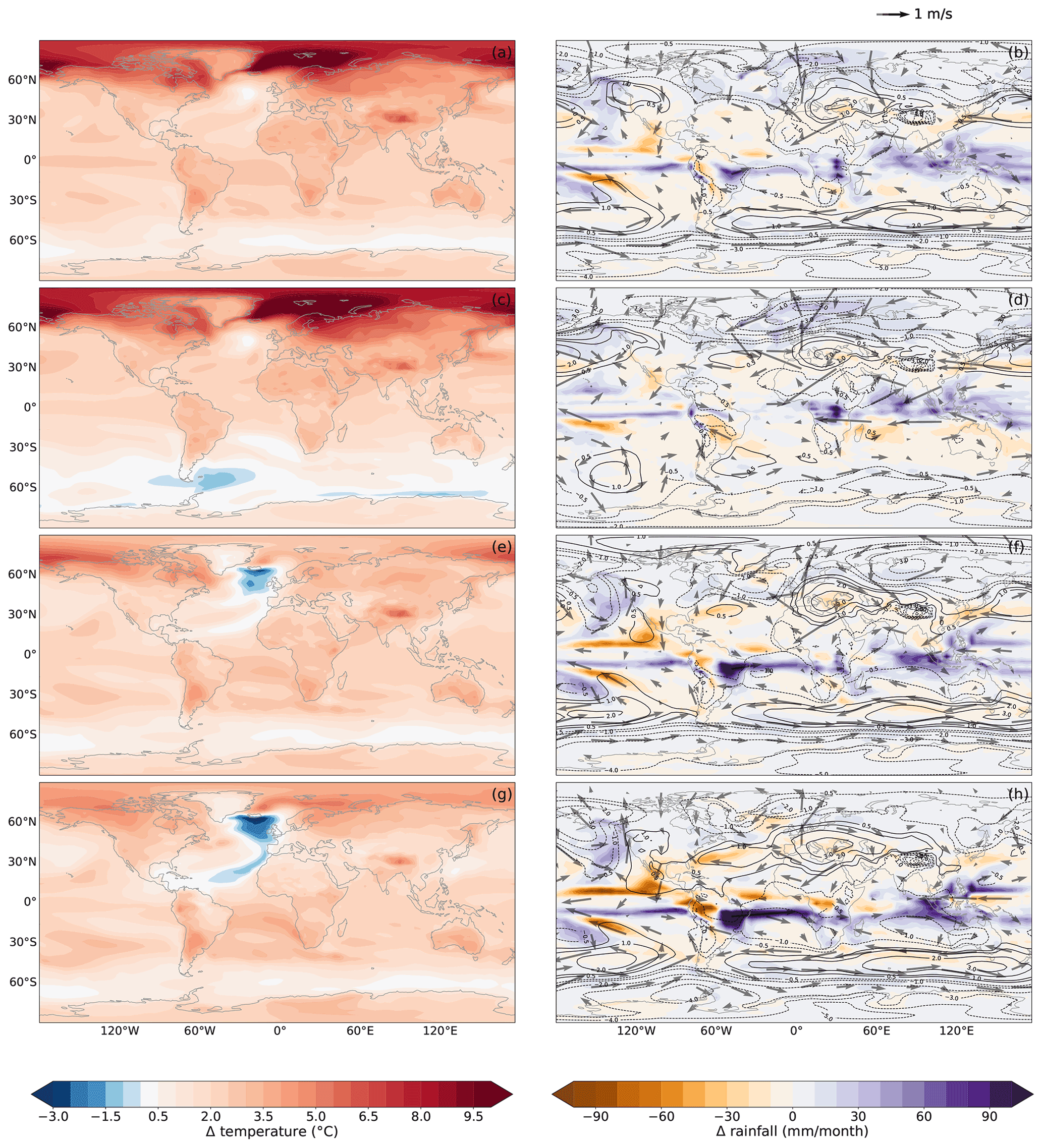
Figure 5Difference between future scenarios (2041–2070) and historical simulation (1976–2005) for the boreal winter season (NDJFM). The left column depicts the surface temperature difference (a, c, e, g), and the right column shows the difference in rainfall (shading), SLP (black contours, dashed lines for negative values) and wind at 850 hPa (vectors) (b, d, f, h). The future scenarios are (a, b) RCP85, (c, d) WAIS3m, (e, f) GrIS1m and (g, h) GrIS3m.
All simulations show a decrease in sea level pressure (SLP) at both poles in boreal summer and winter (Figs. 4 and 5). During boreal summer (MJJAS), there is a decrease in SLP over the Northern Hemisphere, no change in simulated rainfall between 10∘ N and 30∘ S, and an increase in SLP in the Southern Hemisphere between 30 and 60∘ S for the RCP8.5 (Fig. 4b) and WAIS3m (Fig. 4d) simulations. Over the eastern Pacific and tropical Atlantic oceans, the RCP8.5 simulation shows a southward shift of the ITCZ (Fig. 4b). These changes are not simulated in WAIS3m, and a slight increase in rainfall is simulated over this region with more westerly winds (Fig. 4d). In the GrIS1m and GrIS3m simulations, SLP increases near the coasts of Central America and over the southern USA during boreal summer (Fig. 4f and h). A decrease in SLP is simulated between 30 and 60∘ S for GrIS1m (Fig. 4f) and GrIS3m (Fig. 4h) during boreal summer. The resulting inter-hemispheric SLP gradient causes a southward shift of the rain belt (Fig. 4f and h). The SLP gradient between the Southern and Northern Hemisphere increases with the addition of fresh water in the North Atlantic Ocean. This gradient is consistent with an increased southward pressure force that pushes the ITCZ southward over the Atlantic, leading to a significant decrease (increase) in rainfall north (south) of the Equator. A similar mechanism is highlighted during boreal winter (NDJFM) with an increase in precipitation simulated further south over Brazil and southern Africa (Fig. 5f and h).
3.3 Impacts on global monsoon
All model experiments tend to simulate a double Intertropical Convergence Zone (ITCZ), highlighted by the presence of two distinct rain bands over the Pacific Ocean, which is a classical drawback in state-of-the-art GCMs (Fig. 6). Despite this standard bias, the IPSL-CM5 model tends to reproduce the main tropical monsoon areas (shaded areas in Fig. 6) with respect to observed estimates (black contours in Fig. 6). However, the West African and Indian monsoons are simulated too far south, and the model also underestimates rainfall over Central America and northern Australia (Fig. 6). Over the African continent, simulated future changes are moderate over the Sahel for the RCP8.5 (Fig. 6a) and WAIS3m scenario (Fig. 6b). A southward shift of the ITCZ is simulated over the tropical Atlantic region in the GrIS1m (Fig. 6c) and GrIS3m (Fig. 6d) experiments. In GrIS3m, the future rain belt extends further south over southern Africa and southwestern Brazil (Fig. 6d). Most experiments tend to suggest that southeastern US states might become tropical monsoon regions in future. A northward shift of monsoon regions over northern China is also depicted (Fig. 6d).
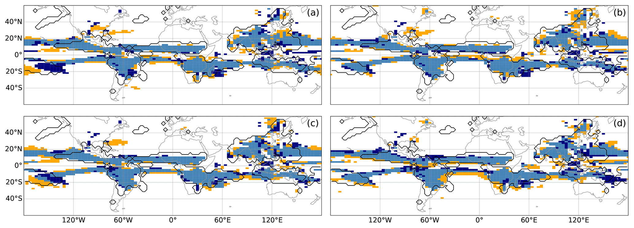
Figure 6Observed (black contour) and simulated (shading) global monsoon regions based on the criterion by Lee and Wang (2014) for (a) RCP8.5, (b) WAIS3m, (c) GrIS1m and (d) GrIS3m. Orange (dark blue) shading depicts monsoon regions simulated for the historical (future) period. Light blue shading shows the monsoon domains that spatially intersect for both periods.
3.4 Impacts on regional monsoons
For the NAMS, rainfall is large from May to September between the Equator and 10∘ N (Fig. 7a). Future RCP8.5 changes reveal a dipole pattern with a decrease in rainfall simulated at the beginning of the rainy season and an increase towards the end (Fig. 7c). The Greenland Ice Sheet melting scenarios amplify these differences (Fig. 7g–i). For GrIS3m, rainfall decreases during the rainy season at 10∘ N (Fig. 7i). For WAIS3m, a slight increase in rainfall is simulated at the beginning of the wet season (Fig. 7e).
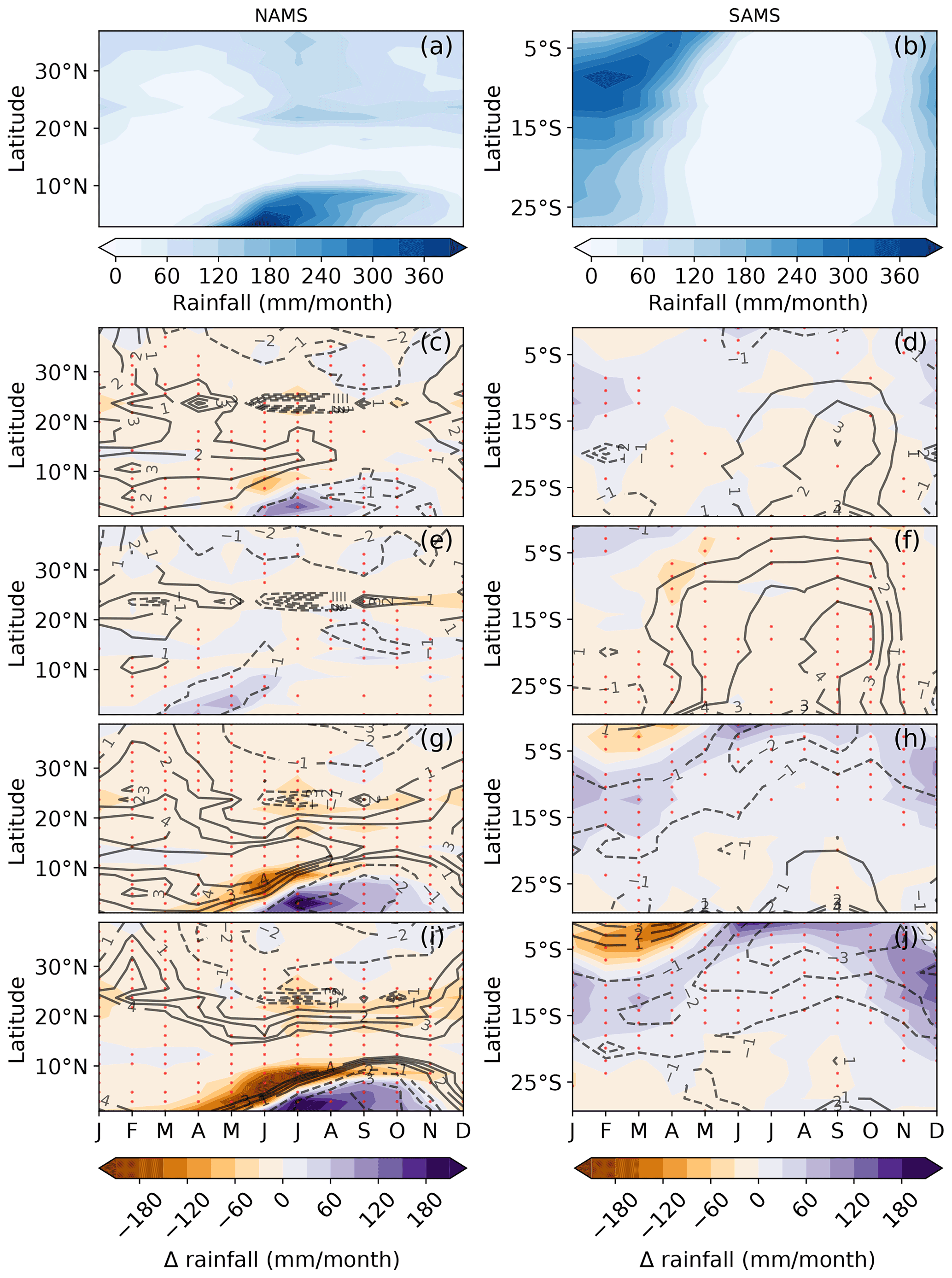
Figure 7Hovmöller diagrams for the American continent domains. The left column corresponds to the NAMS domain (a, c, e, g, i) and the right column to the SAMS domain (b, d, f, h, j). Panels (a, b) correspond to the precipitation values in millimetres per month over the historical period (1976–2005). All other diagrams correspond to the difference between the future scenario (2041–2070) and the historical period (1976–2005) for precipitation (colours) and ΔMSE (black contours, dashed lines for negative values). Future scenarios are (c, d) RCP8.5, (e, f) WAIS3m, (g, h) GrIS1m and (i, j) GrIS3m. Significant differences at the 95 % confidence interval are depicted by red dots according to the Wilcoxon–Mann–Whitney test (see Sect. 2.3).
For the SAMS, the simulated rainy season lasts from October to April, with large rainfall occurring between 5 and 15∘ S (Fig. 7b). For GrIS1m and GrIS3m changes, a rainfall dipole is shown between the Equator and 15∘ S (Fig. 7h–j). Between January and March rainfall intensifies in the southern part. Conversely, a drying signal is simulated over the northern part in future. In addition, future rainfall significantly increases at the beginning of the rainy season (October–December). These changes are more pronounced in the GrIS3m experiment (Fig. 7j). For the RCP8.5 and WAIS3m scenarios, future rainfall changes are much weaker (Fig. 7d–f). The RCP8.5 scenario tends to simulate slightly wetter conditions in future (Fig. 7d). The WAIS3m scenario seems to show an opposite pattern, with a slight increase in precipitation near the Equator and a decrease at 10∘ S (Fig. 7f).
Over the NAF region, two rainy seasons occur over the Gulf of Guinea (April–May and October–November), one rainy season occurs over the Sahel (July–September) and two rainy seasons occur over East Africa (short rains during October–November–December and long rains in March–April–May). The ITCZ first reaches the Guinean coast in April–May, moves northward to reach the Sahel during boreal summer and then quickly retreats southward to reach the Guinean coast in September–October (Fig. 8a). The RCP8.5 and WAIS3m scenarios simulate a slight rainfall increase in April–May near the coast (0–5∘ N) and a larger increase from September to December over 0–10∘ N (Fig. 8c and e). WAIS3m (Fig. 8e) simulates a larger increase from September to December with respect to RCP8.5 (Fig. 8c), and the RCP8.5 scenario simulates moderately drier than average conditions at 7∘ N during the West African monsoon season (July to September). The GrIS1m and GrIS3m scenarios simulate a significant decrease in precipitation over the whole region (Fig. 8g and i). This decrease is larger for the GrIS3m simulation during the West African monsoon season (July–September) at 6–10∘ N (Fig. 8i) and denotes a southward shift of the ITCZ over NAF.
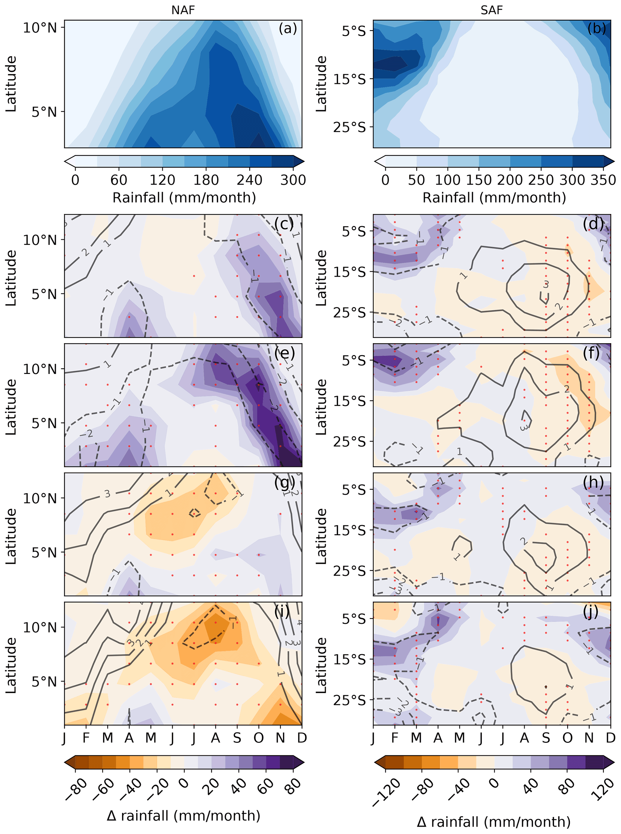
Figure 8Hovmöller diagrams for the African continent domains. The left column corresponds to the NAF domain (a, c, e, g, i) and the right column to the SAF domain (b, d, f, h, j). Panels (a, b) correspond to the precipitation values in millimetres per month over the historical period (1976–2005). All other diagrams correspond to the difference between the future scenario (2041–2070) and the historical period (1976–2005) for precipitation (colours) and ΔMSE (black contours, dashed lines for negative values). Future scenarios are (c, d) RCP8.5, (e, f) WAIS3m, (g, h) GrIS1m and (i, j) GrIS3m. Significant differences at the 95 % confidence interval are depicted by red dots according to the Wilcoxon–Mann–Whitney test (see Sect. 2.3).
For the SAF domain, the rainy season extends from October to March and peaks between 10 and 15∘ S (Fig. 8b). All simulations show an increase in future rainfall between December and May between 15 and 5∘ S (Fig. 8d, f, h, j). RCP8.5 (Fig. 8d) and GrIS scenarios (Fig. 8h–j) simulate a rainfall increase at 15–5∘ S. The RCP8.5 and WAIS3m scenarios simulate drier than average conditions during the onset of the rainy season over southern Africa (Fig. 8d–f). There is a clear southward shift of the ITCZ over the SAF region in GrIS1m and GrIS3m (Fig. 8h–j).
The SAS domain includes both the Indian and Southeast Asian monsoons. Depending on the latitude, rainfall is bimodal in the southern part, with peaks simulated in March and October–November, or unimodal in the northern part with a peak in August (Fig. 9a). The patterns are very similar between the RCP8.5 (Fig. 9b) and WAIS3m (Fig. 9c) scenarios, with an increase in future precipitation simulated from July to December. The melting of the Greenland Ice Sheet tends to buffer this increase in rainfall over SAS (Fig. 9d-e).
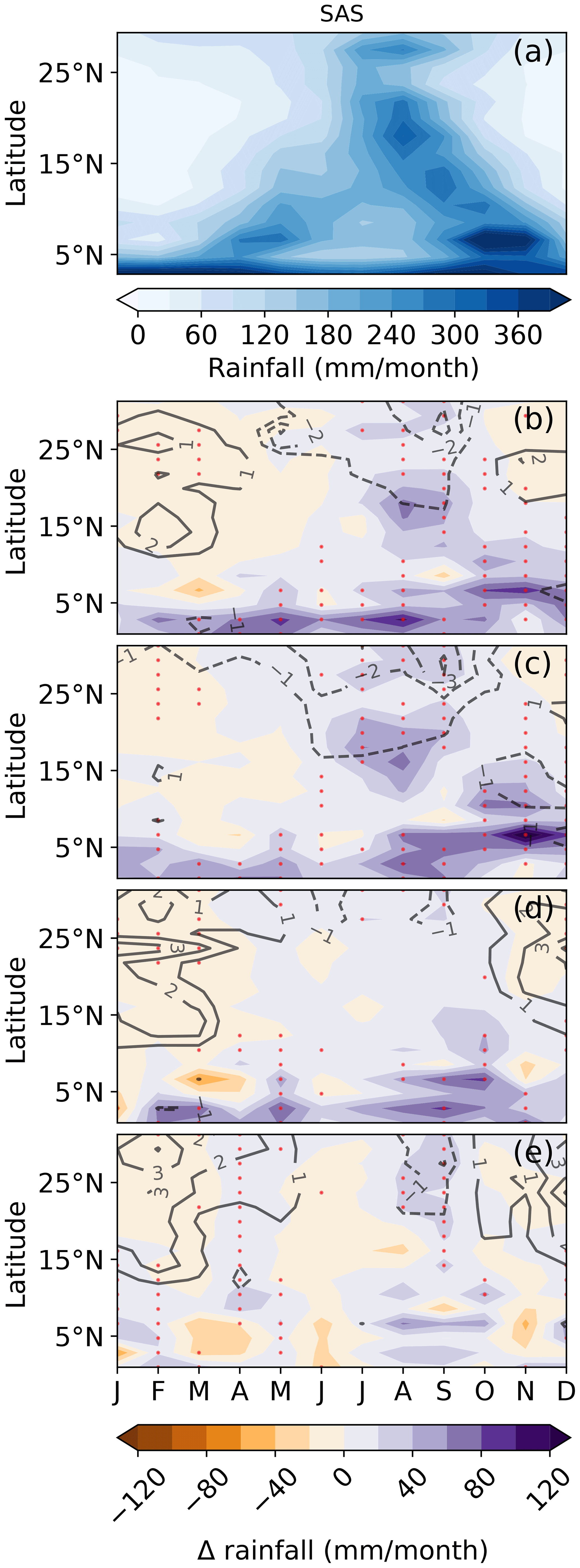
Figure 9Hovmöller diagrams for the SAS domain. Panel (a) corresponds to the precipitation values in millimetres per month over the historical period (1976–2005). All other diagrams correspond to the difference between the future scenario (2041–2070) and the historical period (1976–2005) for precipitation (colours) and ΔMSE (black contours, dashed lines for negative values). Future scenarios are (c, d) RCP8.5, (e, f) WAIS3m, (g, h) GrIS1m and (i, j) GrIS3m. Significant differences at the 95 % confidence interval are depicted by red dots according to the Wilcoxon–Mann–Whitney test (see Sect. 2.3).
For the EAS region, although few points show significant differences, there is little difference between the scenarios (Fig. C1). For the AUSMC region, all scenarios simulate an increase in precipitation in the north (Fig. C1d, f, h, j). This increase extends southwards with the GrIS3m scenario (Fig. C1j). See Appendix C for more information.
As a summary, Greenland ice melt has a strong impact on rainfall seasonality for the NAF and NAMS regions and thus over monsoon regions bordering the North Atlantic. The WAIS3m scenario mainly impacts the seasonality of the North American region and otherwise follows the trends simulated by the RCP8.5 scenario. Changes in rainfall seasonality are linked to changes in the ΔMSE anomaly. When the ΔMSE anomaly increases, atmospheric stability increases and precipitation decreases. Conversely, when the ΔMSE anomaly decreases, atmospheric destabilization and precipitation increase. This relationship between precipitation and MSE is shown for the American (Fig. 7), southern African (Fig. 8d, f, h, j), southern Asian (at high latitudes, see Fig. 9) and Southeast Asian monsoons (Fig. C1c, e, g, i). In some regions, an increase in MSE occurs without an associated decrease in precipitation. This is related to the fact that MSE increases during the dry season when precipitation is already close to zero, as is the case for southern Africa (Fig. 8d, f, h, j), the North American monsoons at high latitudes (Fig. 7c, e, g, i), and the South American monsoon for the RCP8.5 and WAIS3m scenarios (Fig. 7d–f).
Our scenarios suggest that a melting of the ice sheet impacts the quantity, geographical distribution and seasonality of the precipitation supplied to each monsoon system. However, the studied indicators were calculated at a monthly time step, hence not providing detailed information about the frequency and magnitude of potential rainfall extremes and dry spells. In the following we focus on monsoon indicators calculated at a daily time step (see Table 2).
The CDD indicator, representing the length of drought episodes, shows very large inter-annual variability for all scenarios and regions (Fig. 10). Nevertheless, a clear increase in the duration of droughts is shown for the GrIS scenarios over the NAMS region (Fig. 10a). Decreases in the duration of the wet season, the number of rainy days per year and total precipitation (CDWs, R1mm, Pav) are also shown over NAMS by the GrIS scenarios. Changes in the intensity of wet events, characterized by the RX5day and SDII indicators, are moderate over this region (Fig. 10a).
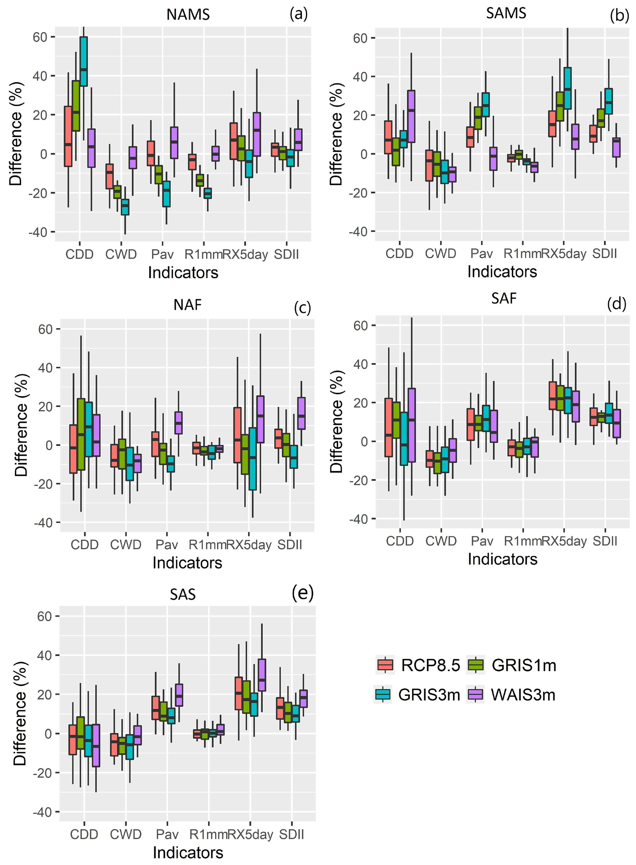
Figure 10Comparison of the inter-annual variability of each land monsoon index for the future period (2041–2070) with the average of the historical period (1976–2005) for (a) NAMS, (b) SAMS, (c) NAF, (d) SAF and (e) SAS as well as for each simulation. RCP8.5 is shown in red, GrIS1m in green, GrIS3m in blue and WAIS3m in purple.
For the SAMS region, changes in CDDs are less marked for the GrIS scenarios with respect to the WAIS3m scenario, which simulates an increase in cumulative dry days (Fig. 10b). An increase in the intensity of precipitation events is shown over SAMS (RX5day, SDII) for the RCP8.5 and GrIS scenarios. Interestingly, the WAIS scenario tends to simulate a decrease in RX5day with respect to the other scenarios. An increase in total rainfall (Pav) is also shown over SAMS (Fig. 10b).
Although the inter-annual variability is very large over the NAF region, the melting of the Greenland Ice Sheet induces an increase in the number of CDDs and a decrease in the number of CWDs for GrIS3m, leading to an overall decrease in total precipitation (Pav) for the GrIS3m scenario (Fig. 10c). Conversely, an increase in extreme precipitation events (RX5day, SDII) and annual precipitation (Pav) is shown for the WAIS3m scenario. More moderate changes are simulated by the RCP8.5 scenario (Fig. 10c).
In the SAF region, there is an intensification of large precipitation events (RX5day, SDII) and a decrease in the number of cumulative wet days and rainy days (CDWs, R1mm) for all simulations (Fig. 10d). Nevertheless, total rainfall (Pav) slightly increases for all scenarios (Fig. 10d)
In SAS region, there is an increase in total precipitation (Pav) for all scenarios linked to an intensification of heavy precipitation events (RX5day, SDII) (Fig. 10e). These changes are largest for the WAIS3M simulation (Fig. 10e).
We investigated the impact of a partial melting of the ice sheet on monsoons and the associated physical mechanisms using the IPSL-CM5 GCM. This model was forced by three hosing scenarios all considering the RCP8.5 scenario as a common radiative forcing. The WAIS3m experiment simulates a melting of the West Antarctic Ice Sheet, and the GrIS experiments simulate a partial melting of the Greenland Ice Sheet equivalent to an additional 1 and 3 m sea level rise. The Greenland Ice Sheet, due to its sub-polar position, releases fresh water directly into the North Atlantic, where cold, dense water sinks to form deep currents. This leads to the slowing of the AMOC, as demonstrated in several studies (Stouffer et al., 2006; Swingedouw et al., 2007; Kageyama et al., 2013; Marzin et al., 2013b). The induced collapse of the AMOC, which we consider to be a major disruption of the thermohaline circulation of the oceans (Vellinga and Wood, 2002), does not occur with the RCP8.5 scenario alone. As shown by Weaver et al. (2012), it is unlikely that the AMOC will undergo an abrupt change when only considering standard RCP scenarios.
The method for water-hosing simulations varies greatly from study to study: the amount of water input and salinity can vary, and simulations can be carried out at different timescales for different climatic contexts (paleoclimates, pre-industrial conditions, future GHG scenarios). The cooling of the North Atlantic induced by the slowing of the AMOC and the subsequent southward shift of the Atlantic ITCZ are robust results shown by many climate models (Vellinga and Wood, 2002; Stouffer et al., 2006; Kageyama et al., 2013; Jackson et al., 2015; Liu et al., 2020) and corroborated by climate proxies (Clement and Peterson, 2008; Mulitza et al., 2008; Marzin et al., 2013b).
Previous studies that do not consider a dynamical evolution of GHGs show a cooling of the Northern Hemisphere and in some cases a warming of the Southern Hemisphere (Vellinga and Wood, 2002; Jackson et al., 2015). In our study, the increase in GHGs leads to a standard global warming signal that is buffered by the slowdown of the AMOC. A rapid melting of the West Antarctic Ice Sheet tends to increase future temperature further at high latitudes in the Northern Hemisphere during boreal winter. Studies that consider changes in GHGs suggest that a shut-down of the AMOC might lead to a return to pre-industrial climate conditions (Vellinga and Wood, 2008), which is not the case in the present study. Liu et al. (2020) also use the baseline RCP8.5 scenario to produce climate sensitivity experiments for which they weaken the AMOC. Their findings are consistent with ours, with a lower temperature increase simulated over the Northern Hemisphere when the AMOC is weakened, a southward shift of the ITCZ and no significant change in the Pacific Ocean. The choice of scenarios and climate models has a strong impact on the robustness of the results as demonstrated by Stouffer et al. (2006). Stouffer et al. (2006) conducted a multi-model analysis in pre-industrial climatic conditions using freshwater inputs of 0.1 and 1 Sv (to compare to 0.22 and 0.68 Sv in our simulations). All climate models simulate a temperature decrease over the northern Atlantic and Greenland, consistently with our findings, but the responses between climate models vary significantly over other regions of the Northern Hemisphere. A southward shift of the ITCZ is also simulated by other climate models, and this change was robust with the addition of +1 Sv. Pressure gradients change, resulting in a north–south pressure force that pushes the rain belt southward; this phenomenon is also confirmed by the proxy studies carried out by Mulitza et al. (2008), Marzin et al. (2013b) and Liu et al. (2020). The addition of fresh water into a hemisphere leads to cooling of that hemisphere, and a southward shift of the ITCZ is simulated in response to freshwater inputs in the North Atlantic regardless of the selected climate model. Regarding the choice of scenario, the northern or southern location of freshwater input plays a crucial role in the seesaw effect. The amount of added water also impacts the intensity of changes. For example, the spatial and temporal trends between the GrIS1m and GrIS3m scenarios are similar but much more pronounced with the latter, for which a larger amount of fresh water is released. For the WAIS3m scenario, the freshwater disturbance tends to be diluted by circumpolar currents in our simulations.
This latitudinal shift leads to significant changes in African climate, with a drying simulated over the Sahel and increased rainfall simulated over the central and southern part of Africa. These results are consistent with the studies by Mulitza et al. (2008), Kageyama et al. (2013) and Liu et al. (2020). A few paleoclimate studies also show an impact of freshwater inputs on the Indian monsoon (Kageyama et al., 2013; Marzin et al., 2013a), but this impact was not evident in our experiments and in results shown by Marzin et al. (2013a). Our study also reveals a southward shift of the American monsoon, with a simulated drying over the central and northern part of South America and a large increase in precipitation over eastern Brazil. Jackson et al. (2015) modify the salinity of the North Atlantic Ocean to produce changes equivalent to freshwater inputs of 10 Sv per year for 10 years. This input in fresh water is much larger than the one used in our study, but it shows similar trends for global temperature changes and a southward shift of the ITCZ, which also impacts the Indo-Pacific basin. Jackson et al. (2015) also emphasize a drying-out of the Amazon, while drier conditions are constrained to the western part of the Amazon basin during austral summer in our GrIS simulations.
Swingedouw et al. (2008) studied the impact of the Antarctica melting over a longer time period (3000 years). They showed that the melting of Antarctica counteracts climatic changes induced by a melting of the Northern Hemisphere ice sheet due to a seesaw mechanism, consistent with former findings by Stocker (1998). In our study, freshwater input in the Southern Hemisphere is diluted by the circumpolar current and has varying impacts in different parts of the world. The impacts of northern and southern freshwater inputs have different impacts on the regional monsoon systems.
The spatial resolution of the IPSL-CM5A-LR climate model is coarse. The slowing trend of the AMOC, the associated decrease in temperature and the southward shift of the rain belt in response to the addition of fresh water into the North Atlantic Ocean are robust results. These changes were found in other studies and are related to large-scale parameters (Mulitza et al., 2008; Kageyama et al., 2013; Jackson et al., 2015; Liu et al., 2020). Concerning freshwater inputs in western Antarctica, a higher-resolution ocean model (at 0.1∘ spatial resolution) could represent oceanic eddies that are not represented in our low-resolution simulations (Kirtman et al., 2012). These eddies occur in the Southern Ocean around Antarctica. These eddies are important sinks of energy between the ocean and the atmosphere, and this sink is more important the further east the wind is (Jullien et al., 2020). Thus, the representation of realistic surface winds in the atmospheric model is also an important issue. These eddies contribute to a global warming signal of about +0.2 ∘C according to Kirtman et al. (2012). This eddy effect is significant but moderate compared to the temperature changes simulated in our ice melt simulations (global cooling between GrIS3m and RCP8.5 of about 0.6 ∘C on average and may reach a maximum of 1.15 ∘C over the period 2041–2070). Jackson et al. (2020) also show that finer spatial resolution can have an impact on the AMOC weakening. Both high- and low-resolution models have significant biases (Chassignet et al., 2020; Jackson et al., 2020). Additional simulations on the impact of horizontal model resolution and bias improvement will be very valuable and useful for improving future climate projections. The impact of the spatial resolution is more important at regional scale. Therefore, for the Asian and AUSMC regions it is difficult to simulate reliable trends. The presence of the Himalayas, which has a strong impact on the Asian monsoon (Boos and Kuang, 2010), is poorly represented in our model simulations due to a resolution that is too coarse, and very few island grid boxes are available in the AUSMC region to obtain reliable results. Our findings based on a low-spatial-resolution model still simulate realistic monsoon dynamics, and simulated future changes are in agreement with other published studies (Mulitza et al., 2008; Kageyama et al., 2013; Jackson et al., 2015; Liu et al., 2020).
The IPSL-CM5 model belongs to the CMIP5 intercomparison exercise, whose parameterization has evolved for the CMIP6 framework (Boucher et al., 2020). The transition from CMIP5 to CMIP6 has led to changes in many GCMs, with reduced biases and uncertainties in many regions of the world. The presence of a double ITCZ is a persistent bias in the different intercomparison exercises; however, this bias has been reduced in CMIP6 (Tian and Dong, 2020). The representation of monsoons by GCMs has improved between CMIP5 and CMIP6 for China (Xin et al., 2020), India (Gusain et al., 2020), East Asia (Xin et al., 2020) and East Africa, although there are still significant errors (Ayugi et al., 2021). For the Sahel, future rainfall uncertainties remain large despite the evolution of GCMs (Monerie et al., 2020). For Central America and South America, there is a large dispersion across the different climate models utilized in CMIP5 and CMIP6, with, however, a slight improvement in CMIP6 GCMs (Ortega et al., 2021). It is noteworthy that the multi-model average is often closer to reality than each model considered independently (Ayugi et al., 2021). Significant changes in rainfall seasonality are simulated by the IPSL-CM5 model as well as in the CMIP5 and CMIP6 intercomparison exercises (Wainwright et al., 2021). In our methodological framework, freshwater input is added continuously between 2020 and 2070. However, the melting and release of fresh water might be highly non-linear (tipping point) and may vary seasonally. Sensitivity climate experiments that consider different values of freshwater input depending on the season would allow a more realistic simulation.
Although the transition from CMIP5 to CMIP6 has led to improvements in climate simulation in many regions of the world, the models still have systematic errors in the simulation of precipitation.
The most extreme emission scenario, RCP8.5, was used in this study. The choice of RCP8.5 as a credible scenario for the 21st century has been recently criticized by Hausfather and Peters (2020). Hausfather and Peters (2020) argue that real-word GHG emissions, in order to reach the RCP8.5 scenario, would require an increase in coal use beyond recoverable and available reserves. They also note that even without climate policies, as assumed in RCP8.5, clean energy costs tend to decrease over time. Consequently, they advise that the RCP8.5 scenario should not be used as a most likely future scenario, but only as an extreme one (Hausfather and Peters, 2020). The potential large number of retroactive events in snow-covered regions resulting from rising temperatures (Fettweis et al., 2013) suggests that tipping points can be very rapid and sudden. Recent trends are worrying: the recent melting of the A68 iceberg was estimated to have released about 152 Gt of fresh water and nutrients near South Georgia (Braakmann-Folgmann et al., 2022). In addition, nearly twice as much lightning was detected north of 80∘ N in 2021 than in the previous 9 years combined, denoting an increase in liquid precipitation at high latitudes (Network, 2022). We only investigated the impact of ice sheet melting, but a melting of the permafrost, which would potentially release a large amount of methane into the atmosphere, is worth investigating (Stendel and Christensen, 2002). As perspectives, multi-model studies of tipping point scenarios (e.g. ice sheet melting, melting of the permafrost, dieback of the Amazon) and their potential impacts on societies should be encouraged (Lenton et al., 2019). Rising sea levels and induced climatic impacts could have primordial consequences for human societies, health (Chemison et al., 2021), agriculture (Defrance et al., 2017) and the global economy (Kuhlbrodt et al., 2009).
All experiments are based on the first ensemble member r1i1p1. Only one simulation was carried out for each ice melt experiment because of the magnitude of the added freshwater signal. To compare simulations, only a single ensemble member was used to avoid smoothing out internal variability of the model. In the following figures we compare global mean temperature and rainfall for all ensemble members available for the historical (Fig. A1) and RCP8.5 (Fig. A2) scenario carried out with the IPSL-CM5A-LR model. All historical and RCP8.5 scenario experiments simulate a warming–wetting trend. The spread between ensemble members is relatively moderate, and the ice melting experiments (GrIS1m, GrIS3m and WAIS3m, with colder and drier conditions) clearly stand out from the internal model variability derived for all RCP8.5 simulations (Fig. A2).
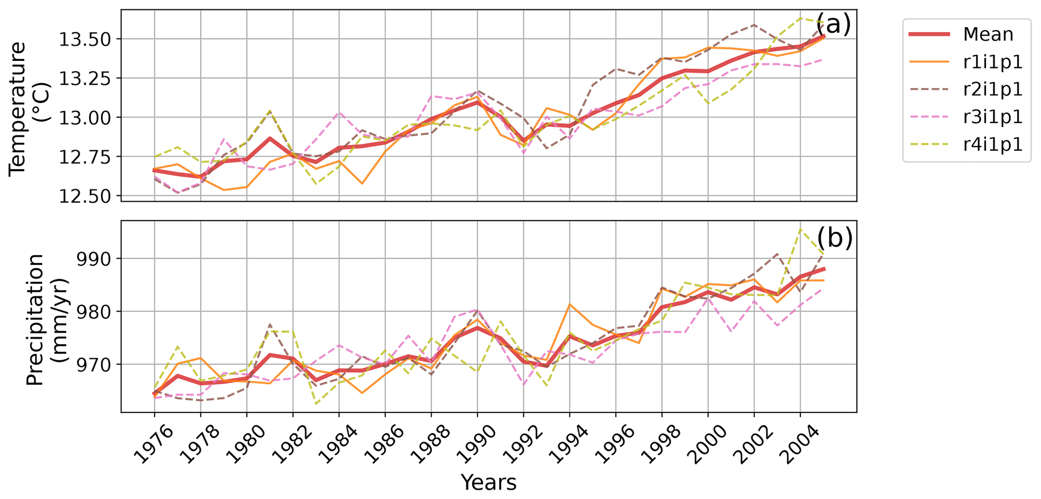
Figure A1Temporal evolution of (a) temperature and (b) precipitation over the historical period (1976–2005) for the different ensemble members. The solid orange line depicts the historical simulation used in the study. The thick red line shows the ensemble mean of all simulations from r1i1p1 to r4i1p1.
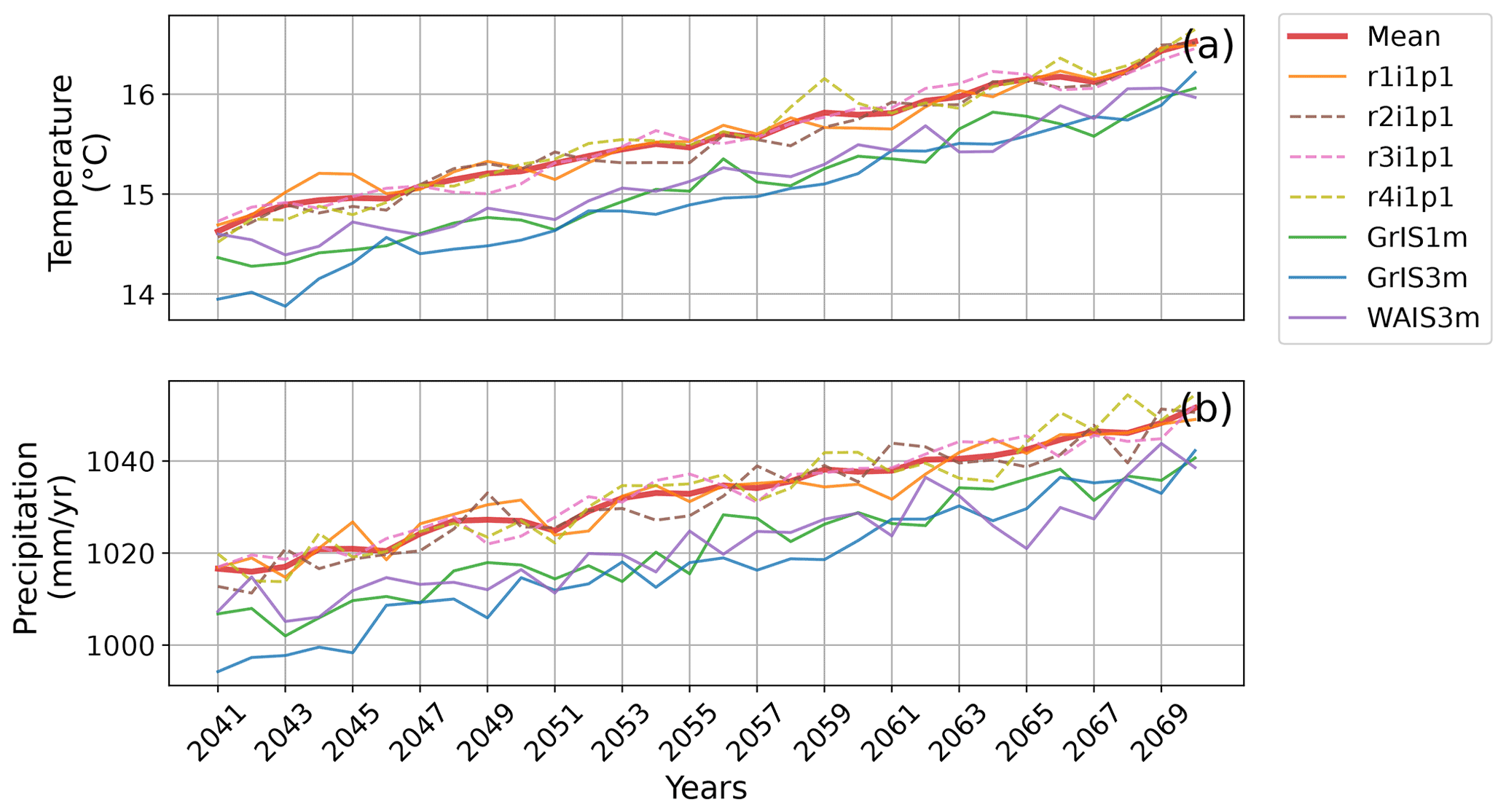
Figure A2Temporal evolution of (a) temperature and (b) precipitation over the future period (2041–2070) for the different RCP8.5 runs (r1i1p1, r2i1p1, r3i1p1, r4i1p1) and for the different ice melt simulations (GrIS1m, GrIS3m, WAIS3m). The solid orange line depicts the RCP8.5 simulation used in the study. The thick red line shows the ensemble mean of all RCP8.5 simulations from r1i1p1 to r4i1p1.
The difference in stream function between future and historical periods is slight affected by seasonality in our simulations (Figs. B1 and B2). Our simulation provides continuous fresh water between 2020 and 2070 without seasonal variations. This may explain why there is small seasonal difference for the simulations with ice melt (Figs. B1b–d and B2b–d). The GrIS1m and GrIS3m simulations still show larger maximum differences during the boreal summer located in the Northern Hemisphere (Figs. B1c, d and B2c, d). In contrast, for the Southern Hemisphere, the maximum difference for the GrIS simulations appears to be reached during boreal winter (Figs. B1c, d and B2c, d).
The differences in sea ice fraction (%) between our different future scenarios (2041–2070) and the historical simulation (1976–2005) for boreal winter are shown in Fig. B3 and austral winter in Fig. B4. The temporal evolution of sea ice fraction and temperature for our different simulations for the Northern Hemisphere is presented in Fig. B5 and for the Southern Hemisphere in Fig. B6. To calculate indices, the sea ice area was defined as follows: any grid point with a 30-year median (1976–2005) ≥ 15 % sea ice. This analysis was done by seasons (MJJAS and NDJFM) and for each hemisphere. The largest ice melting is simulated for the RCP8.5 and WAIS simulations in the Northern Hemisphere during boreal winter (Figs. B3a, b and B5a, c). The addition of fresh water in GrIS experiments tends to limit future ice melting around Greenland (Figs. B3c, d and B5a–c). Most future experiments tend to simulate ice melting over western Antarctica, while more ice is simulated over southeastern Antarctica (Figs. B4a, c, d and B6a–c). These findings are consistent with results from the IPCC AR6 report (Fox-Kemper et al., 2021). Conversely, the WAIS experiments simulate more ice over the western part of Antarctica and a decreased sea ice extent over northeastern Antarctica (Fig. B4b). The addition of fresh water in the northern Atlantic leads to colder temperatures (Fig. B5b–d), a decreased AMOC and a more moderate sea ice melting (Fig. B5a–c). A similar relationship is shown over the Southern Hemisphere for the WAIS3m experiment (Fig. B6). There is no clear lag between simulated temperatures and sea ice extent, so we assume that this process is related to the coupling between the atmosphere, the ocean and the cryosphere.
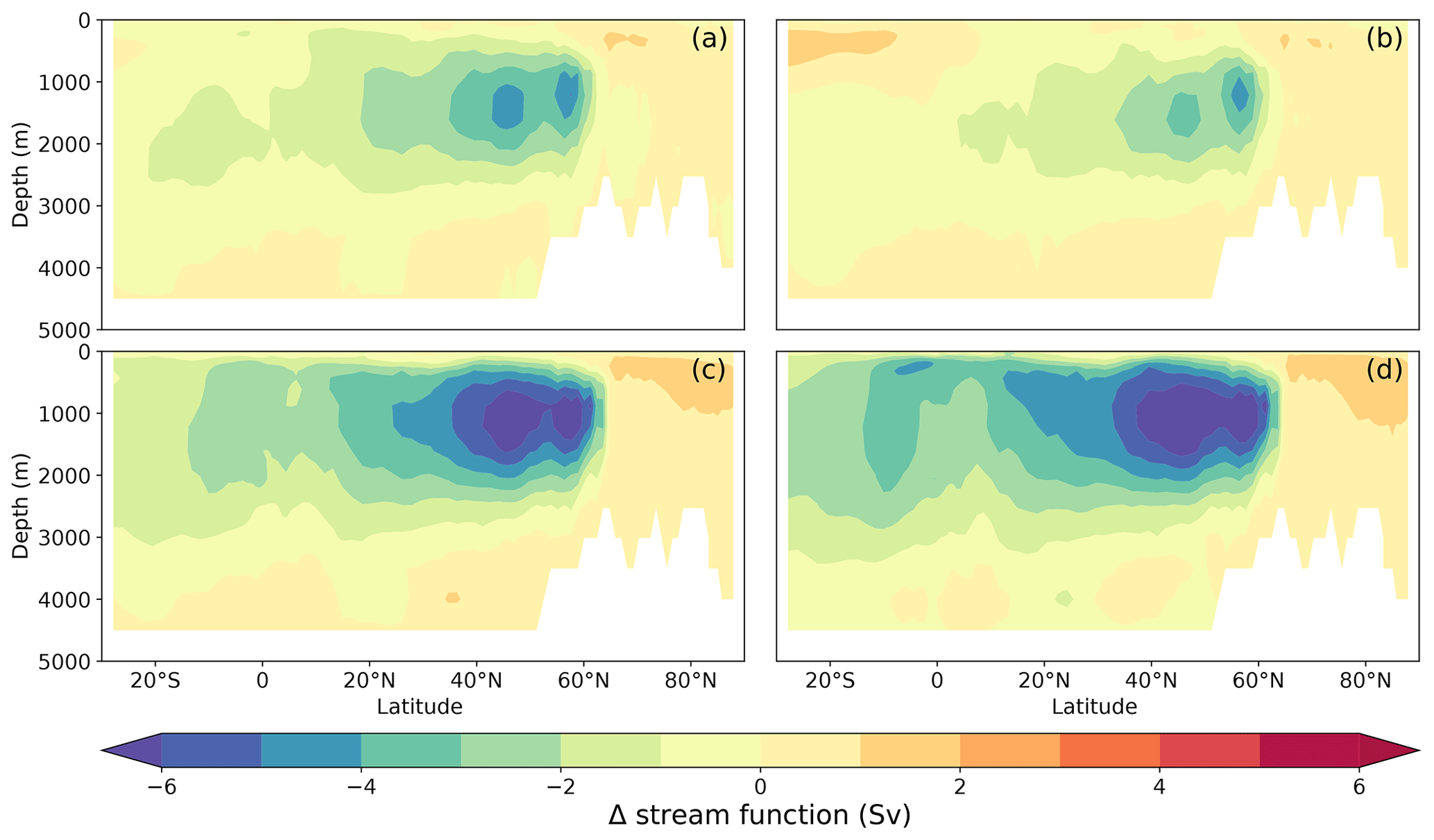
Figure B1Stream function difference between future scenarios (2041–2070) and historical simulation (1976–2005) for the MJJAS season. The future scenarios are (a) RCP8.5, (b) WAIS3m, (c) GrIS1m and (d) GrIS3m.
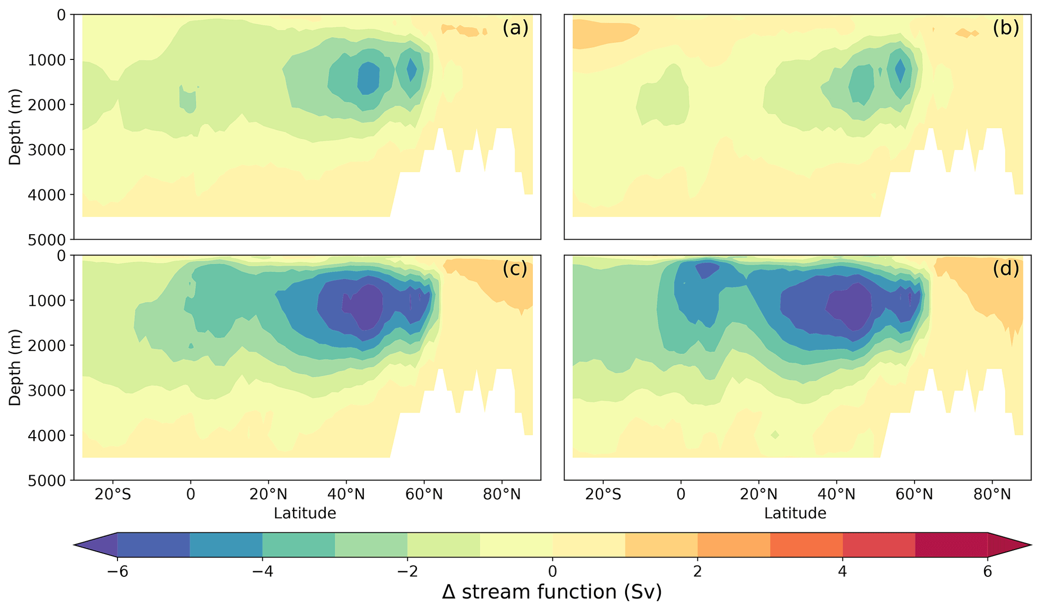
Figure B2Stream function difference between future scenarios (2041–2070) and historical simulation (1976–2005) for the NDJFM season. The future scenarios are (a) RCP8.5, (b) WAIS3m, (c) GrIS1m and (d) GrIS3m.
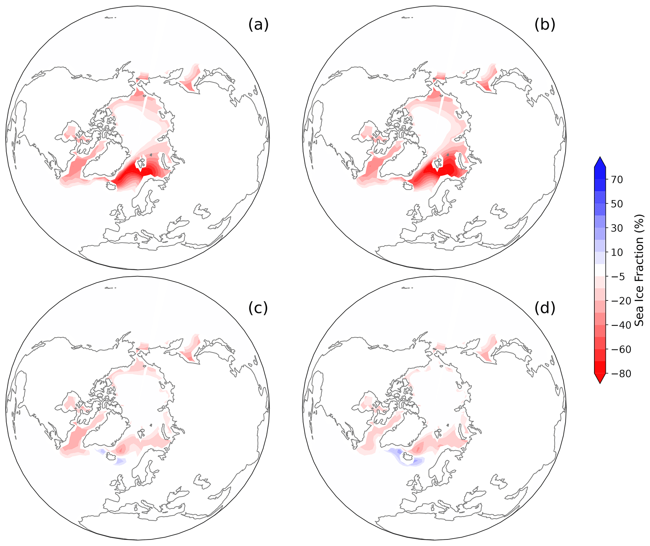
Figure B3Sea ice fraction difference (%) between future scenario (2041–2070) (a) RCP8.5, (b) WAIS3m, (c) GrIS1m, (d) GrIS3m and historical simulation (1976–2005) for the Northern Hemisphere in NDJFM.
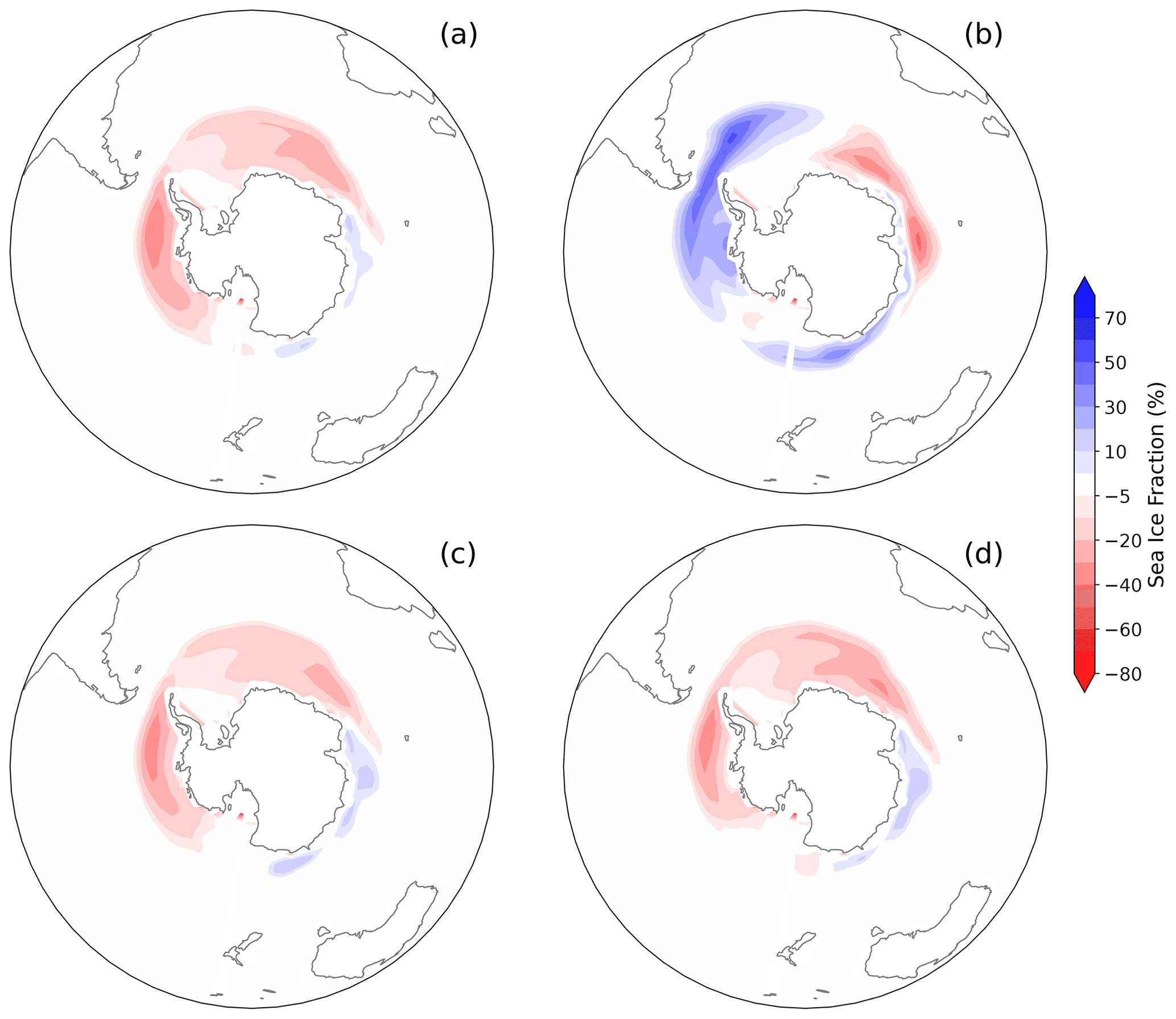
Figure B4Sea ice fraction difference (%) between future scenario (2041–2070) (a) RCP8.5, (b) WAIS3m, (c) GrIS1m, (d) GrIS3m and historical simulation (1976–2005) for the Southern Hemisphere in MJJAS.

Figure B5Temporal evolution of (a–c) sea ice fraction (%) and (b–d) temperature (∘C) in the Northern Hemisphere for (a, b) NDJFM and (c, d) MJJAS. The orange dotted line represents the 0 ∘C isotherm.
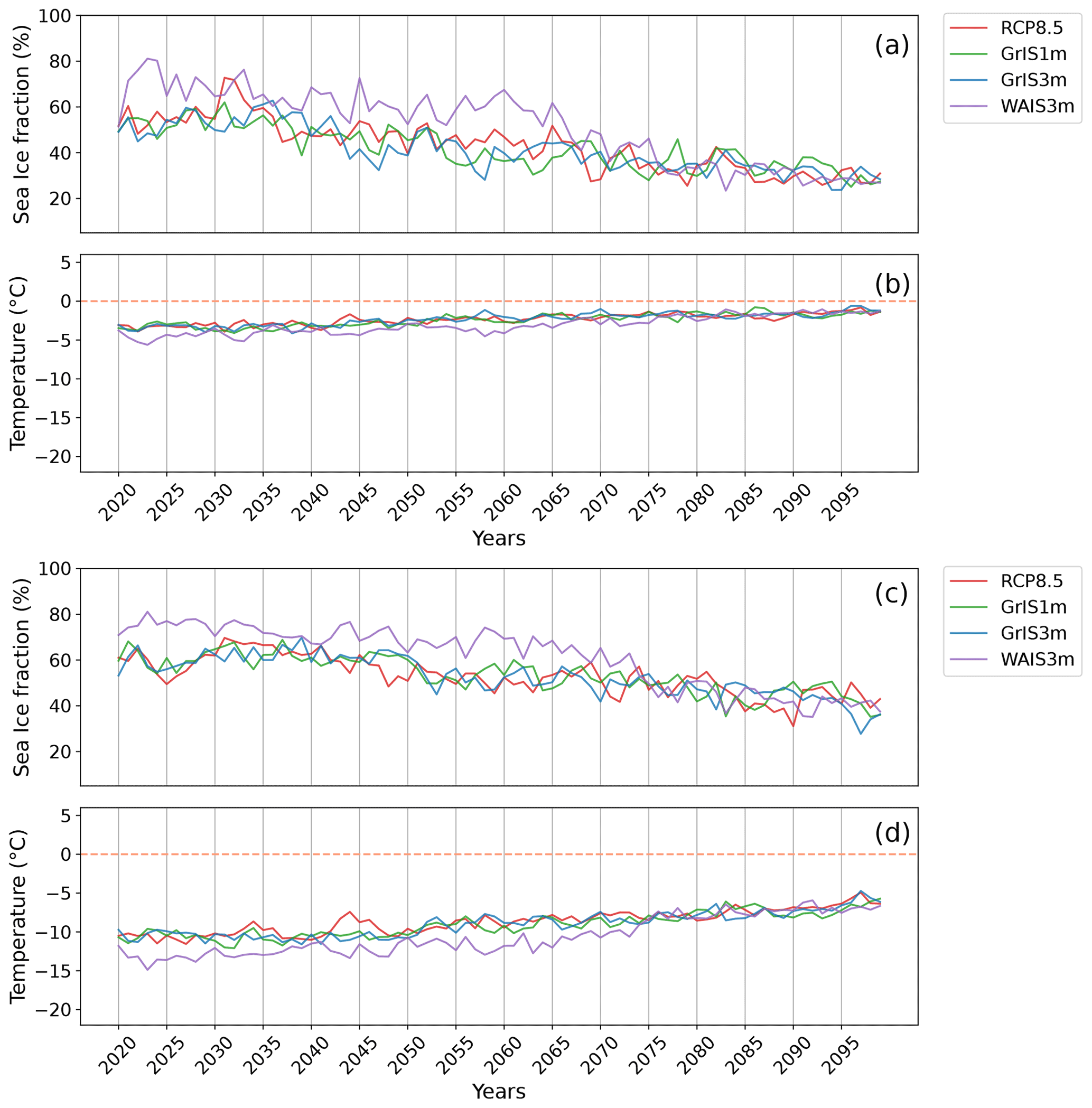
Figure B6Temporal evolution of (a–c) sea ice fraction (%) and (b–d) temperature (∘C) in the Southern Hemisphere for (a–b) NDJFM and (c–d) MJJAS. The orange dotted line represents the 0 ∘C isotherm.
For the EAS region, the wet season extends from May to August with maximum rainfall simulated over the south in July (Fig. C1a). Although only a few points show significant differences, there is still little difference between the scenarios when comparing future and historical periods (Fig. C1a, c, e, g, i). All experiments simulate a decrease in precipitation during boreal winter. During summer, there is an increase in precipitation in the north. In the south, there is a decrease in precipitation during winter but also at the beginning of the wet season, whereas there is an increase in precipitation at the end of the wet season. (Fig. C1c, e, g, i).
To validate the use of the different monsoon indicators for each study region, indices for the historical period are compared with those obtained for the EWEMBII data. For CDDs, the values obtained are close between the two datasets, although the values from the historical simulations have a slight negative bias for the East Asian, North American and southern African regions (Fig. C2a). For the CDW, all regions have a slight negative bias with the historical simulation (Fig. C2b). This bias is also shown for the RX5day indicator (Fig. C2e) but is not found with the Pav, R1mm and SDII indicators, which have very similar values between the two datasets (Fig. C2c, d, f). Despite a slight negative bias for some indicators in some regions, the indicators show the same trends between the two datasets (Fig. C2).
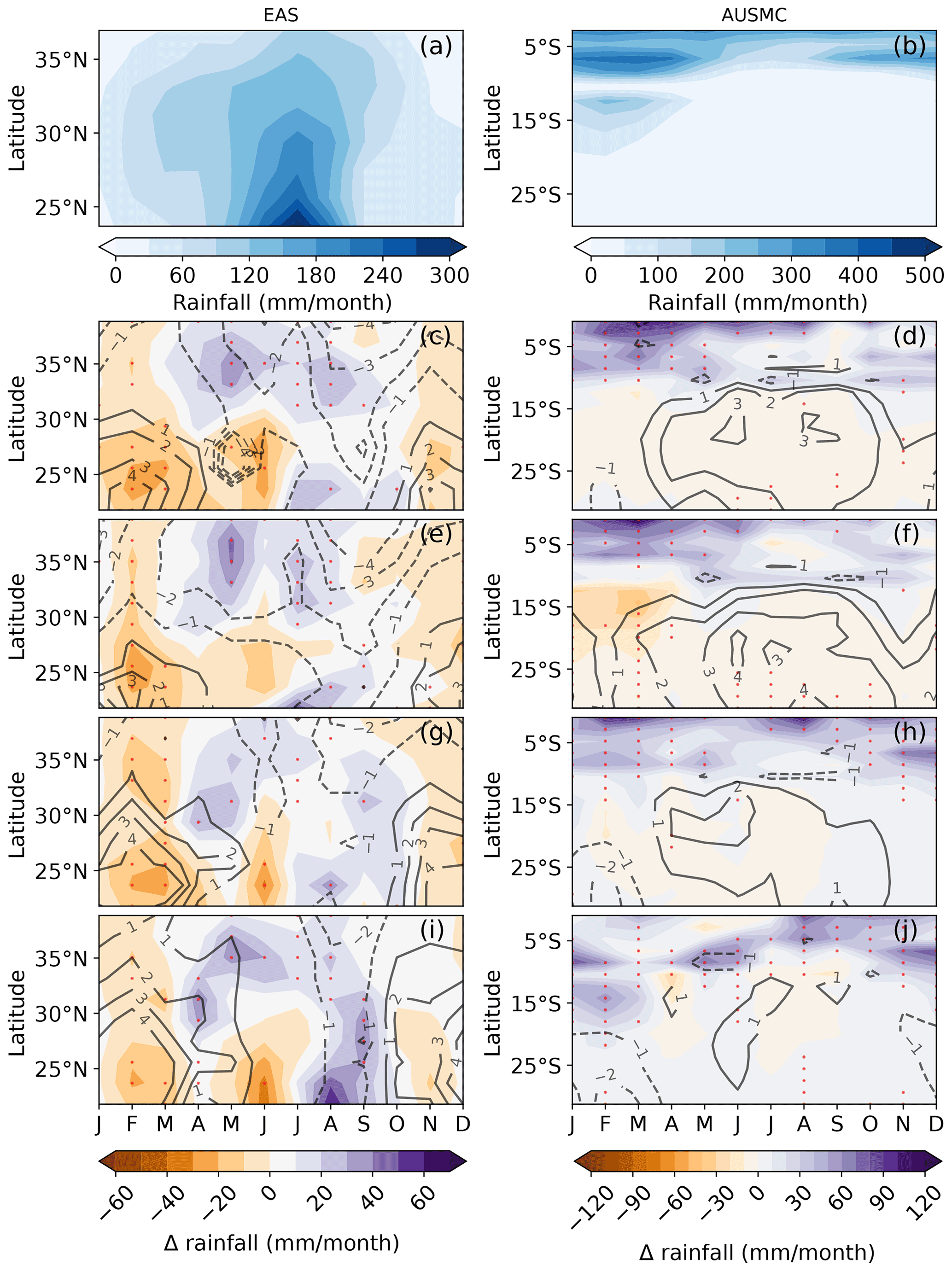
Figure C1Hovmöller diagrams. The left column corresponds to the EAS domain (a, c, e, g, i) and the right column to the AUSMC domain (b, d, f, h, j). Panels (a, b) correspond to the precipitation values in millimetres per month over the historical period (1976–2005). All other diagrams correspond to the difference between the future scenario (2041–2070) and the historical period (1976–2005) for precipitation (colours) and ΔMSE (black contours, dashed lines for negative values). Future scenarios are (c, d) RCP8.5, (e, f) WAIS3m, (g, h) GrIS1m and (i, j) GrIS3m. Significant differences at the 95 % confidence interval are depicted by red dots according to the Wilcoxon–Mann–Whitney test (see Sect. 2.3).
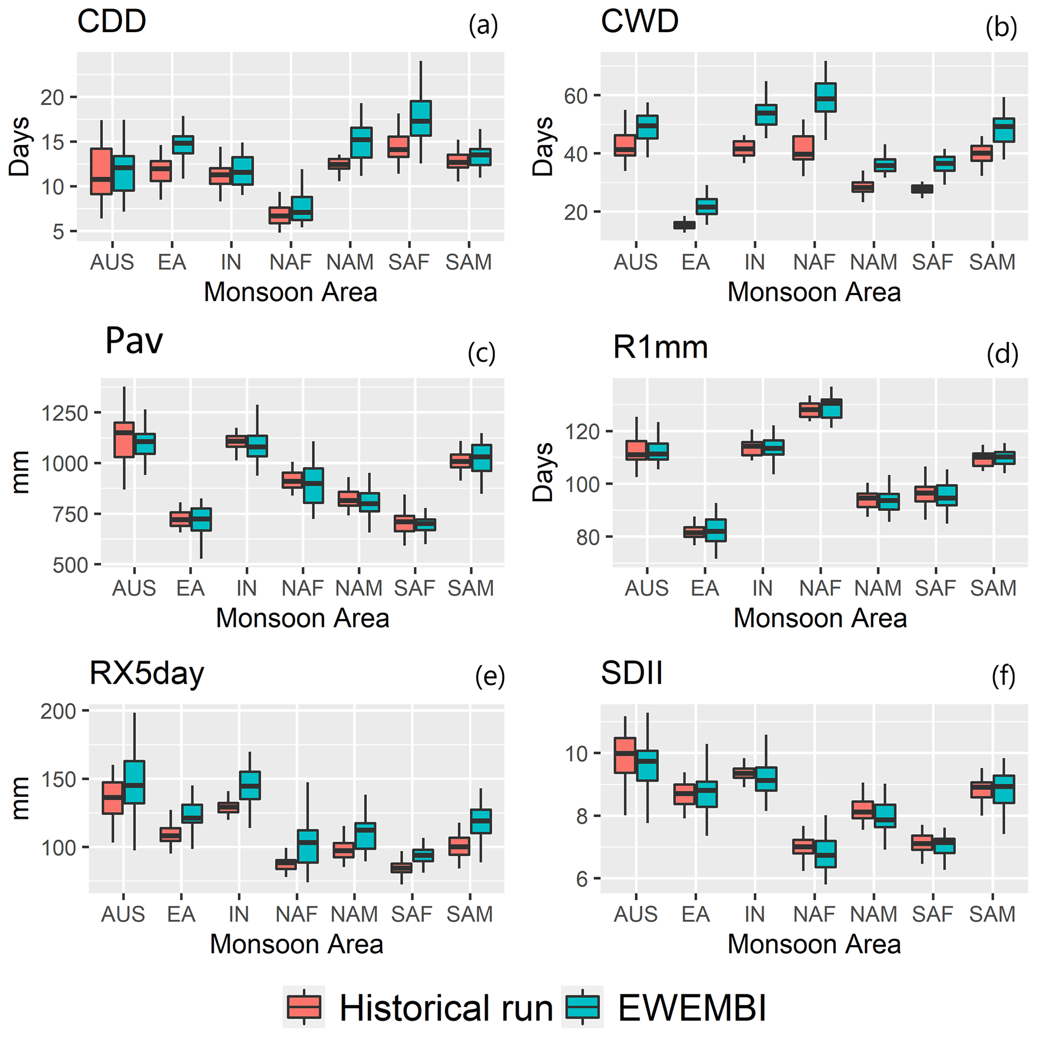
Figure C2Comparison of the inter-annual variability of each monsoon index for the period 1976–2005 for the historical run simulation (red) and EWEMBI data (blue) for each monsoon system and for each monsoon indicator: (a) CDDs, (b) CDW, (c) Pav, (d) R1mm, (e) RX5day, (f) SDII.
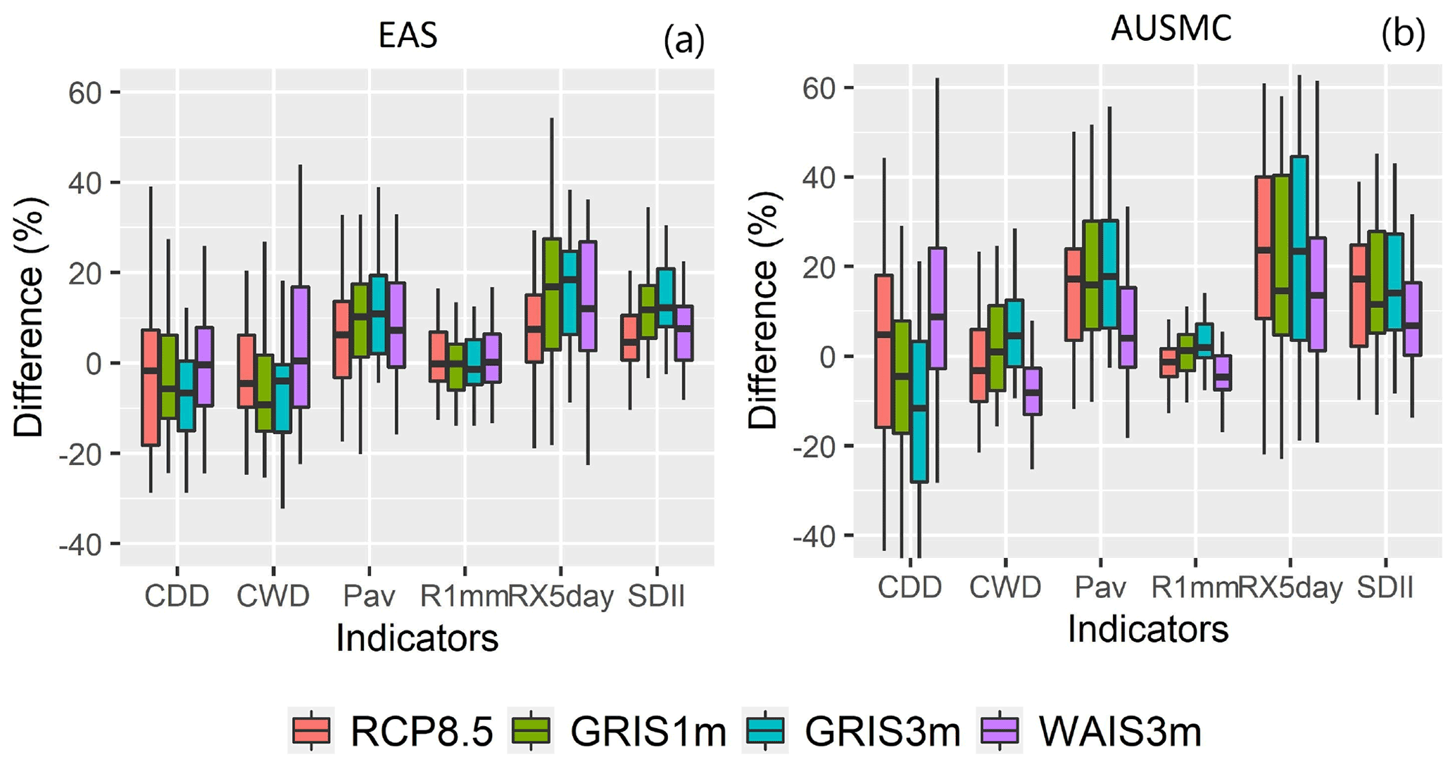
Figure C3Comparison of the inter-annual variability of each monsoon index for the future period (2041–2070) with the average of the historical period (1976–2005) for each monsoon system: (a) EAS, (b) AUSMC.
For the EAS region, there are almost no changes in the different monsoon indexes for all scenarios, with only a slight increase in total precipitation (Pav) due to an intensification of precipitation events (RX5day, SDII) (Fig. C3a).
For the AUSMC region, very high inter-annual variability is shown (Fig. C3b). Total precipitation (Pav) increases slightly for the RCP8.5, GrIS1m and GrIS3m scenarios, which may be related to a decrease in the duration of the dry season (CDDs) and an intensification of precipitation events (RX5day, SDII) (Fig. C3b).
The climate model code used for this study, IPSL-CM5A-LR, can be accessed via this web page: http://forge.ipsl.jussieu.fr/igcmg_doc/wiki/Doc/Install (IGCMG, 2022).
All simulations that support the findings of this study are available at https://doi.org/10.17605/OSF.IO/YTER9 (Chemison et al., 2022), which should allow reproducibility of the main figures. For the indices, the data are available at https://doi.org/10.17632/fbsdj87gjg.2 (Defrance, 2022).
AC wrote the article and produced most of the figures and analysis. DD carried out the WAIS3m, GrIS1m and GrIS3m simulations and produced figures. GR and CC guided the analysis and contributed to the writing of the paper.
The contact author has declared that none of the authors has any competing interests.
Publisher's note: Copernicus Publications remains neutral with regard to jurisdictional claims in published maps and institutional affiliations.
We acknowledge the Direction de la Recherche Fondamentale (DRF) of the Commissariat à l'énergie atomique et aux énergies alternatives (CEA) for Alizée Chemison's PhD funding and the DRF Impulsion programme for funding the EPICLIM project awarded to Gilles Ramstein. We also thank Masa Kageyama for all her help in writing this paper.
This research work was funded by a PhD grant from the Direction de la Recherche Fondamentale (DRF) of the Commissariat à l’énergie atomique et aux énergies alternatives (CEA, the French Atomic Energy and Alternative Energies Commission) and by the EPICLIM project awarded to Gilles Ramstein by the DRF Impulsion programme.
This paper was edited by Anping Chen and reviewed by three anonymous referees.
Adler, R. F., Sapiano, M. R., Huffman, G. J., Wang, J.-J., Gu, G., Bolvin, D., Chiu, L., Schneider, U., Becker, A., Nelkin, E., Xie, P., Ferraro, R., and Shin, D.-B.: The Global Precipitation Climatology Project (GPCP) monthly analysis (new version 2.3) and a review of 2017 global precipitation, Atmosphere, 9, 138, https://doi.org/10.3390/atmos9040138, 2018. a
Aumont, O. and Bopp, L.: Globalizing results from ocean in situ iron fertilization studies, Global Biogeochem. Cy., 20, GB2017, https://doi.org/10.1029/2005GB002591, 2006. a
Ayugi, B., Jiang, Z., Zhu, H., Ngoma, H., Babaousmail, H., Karim, R., and Dike, V.: Comparison of CMIP6 and CMIP5 models in simulating mean and extreme precipitation over East Africa, Int. J. Climatol., 41, 6474–6496, https://doi.org/10.1002/joc.7207, 2021. a, b
Bakker, P., Schmittner, A., Lenaerts, J., Abe-Ouchi, A., Bi, D., van den Broeke, M., Chan, W.-L., Hu, A., Beadling, R., Marsland, S. J., Mernild, S. H., Saenko, O. A., Swingedouw, D., Sullivan, A., and Yin, J.: Fate of the Atlantic Meridional Overturning Circulation: Strong decline under continued warming and Greenland melting, Geophys. Res. Lett., 43, 12252–12260, https://doi.org/10.1002/2016GL070457, 2016. a
Biasutti, M.: Forced Sahel rainfall trends in the CMIP5 archive, J. Geophys. Res.-Atmos., 118, 1613–1623, 2013. a
Biasutti, M. and Sobel, A. H.: Delayed Sahel rainfall and global seasonal cycle in a warmer climate, Geophys. Res. Lett., 36, L23707, https://doi.org/10.1029/2009GL041303, 2009. a, b
Biasutti, M., Sobel, A. H., and Camargo, S. J.: The role of the Sahara low in summertime Sahel rainfall variability and change in the CMIP3 models, J. Climate, 22, 5755–5771, 2009. a
Boos, W. R. and Kuang, Z.: Dominant control of the South Asian monsoon by orographic insulation versus plateau heating, Nature, 463, 218–222, 2010. a
Boucher, O., Servonnat, J., Albright, A. L., Aumont, O., Balkanski, Y., Bastrikov, V., Bekki, S., Bonnet, R., Bony, S., Bopp, L., Braconnot, P., Brockmann, P., Cadule, P., Caubel, A., Cheruy, F., Codron, F., Cozic, A., Cugnet, D., D'Andrea, F., Davini, P., de Lavergne, C., SDenvil, S., Deshayes, J., Devilliers, M., Ducharne, A., Dufresne, J.-L., Dupont, E., Éthé, C., Fairhead, L., Falletti, L., Flavoni, S., Foujols, M.-A., Gardoll, S., Gastineau, G., Ghattas, J., Grandpeix, J.-Y., Guenet, B., Lionel, Guez, E., Guilyardi, E., Guimberteau, M., Hauglustaine, D., Hourdin, F., Idelkadi, A., Joussaume, S., Kageyama, M., Khodri, M., Krinner, G., Lebas, N., Levavasseur, G., Lévy, C., Li, L., Lott, F., Lurton, T., Luyssaert, S., Madec, G., Madeleine, J.-B., Maignan, F., Marchand, M., Marti, O., Mellul, L., Meurdesoif, Y., Mignot, J., Musat, I., Ottlé, C., Peylin, P., Planton, Y., Polcher, J., Rio, C., Rochetin, N., Rousset, C., Sepulchre, P., Sima, A., Swingedouw, D., Thiéblemont, R., Khadre Traore, A., Vancoppenolle, M., Vial, J., Vialard, J., Viovy, N., and Vuichard, N.: Presentation and evaluation of the IPSL-CM6A-LR climate model, J. Adv. Model. Earth Syst., 12, e2019MS002010, https://doi.org/10.1029/2019MS002010, 2020. a
Braakmann-Folgmann, A., Shepherd, A., Gerrish, L., Izzard, J., and Ridout, A.: Observing the disintegration of the A68A iceberg from space, Remote Sens. Environ., 270, 112855, https://doi.org/10.1016/j.rse.2021.112855, 2022. a
Broecker, W., Bond, G., Klas, M., Clark, E., and McManus, J.: Origin of the northern Atlantic's Heinrich events, Clim. Dynam., 6, 265–273, https://doi.org/10.1007/BF00193540, 1992. a
Cavazos, T., Turrent, C., and Lettenmaier, D.: Extreme precipitation trends associated with tropical cyclones in the core of the North American monsoon, Geophys. Res. Lett., 35, L21703, https://doi.org/10.1029/2008GL035832, 2008. a
Chassignet, E. P., Yeager, S. G., Fox-Kemper, B., Bozec, A., Castruccio, F., Danabasoglu, G., Horvat, C., Kim, W. M., Koldunov, N., Li, Y., Lin, P., Liu, H., Sein, D. V., Sidorenko, D., Wang, Q., and Xu, X.: Impact of horizontal resolution on global ocean–sea ice model simulations based on the experimental protocols of the Ocean Model Intercomparison Project phase 2 (OMIP-2), Geosci. Model Dev., 13, 4595–4637, https://doi.org/10.5194/gmd-13-4595-2020, 2020. a
Chemison, A., Ramstein, G., Tompkins, A. M., Defrance, D., Camus, G., Charra, M., and Caminade, C.: Impact of an accelerated melting of Greenland on malaria distribution over Africa, Nat. Commun., 12, 1–12, https://doi.org/10.1038/s41467-021-24134-4, 2021. a
Chemison, A., Defrance, D., Ramstein, G., and Caminade, C.: Simulation files to reproduce the paper “Impact of an acceleration of ice sheet melting on monsoon systems”, OSFH [data set], https://doi.org/10.17605/OSF.IO/YTER9, 2022. a, b
Cheng, W., Chiang, J. C., and Zhang, D.: Atlantic meridional overturning circulation (AMOC) in CMIP5 models: RCP and historical simulations, J. Climate, 26, 7187–7197, https://doi.org/10.1175/JCLI-D-12-00496.1, 2013. a, b
Christensen, J. H., Kanikicharla, K. K., Aldrian, E., An, S. I., Cavalcanti, I. F. A., de Castro, M., Dong, W., Goswami, P., Hall, A., Kanyanga, J. K., Kitoh, A., Kossin, J., Cheung Lau, N., Renwick, J., Stephenson, D. B., Ping Xie, S., Zhou, T., Abraham, L., Ambrizzi, T., AndersonOsamu Arakawa, B., Arritt, R., Baldwin, M., Barlow, M., Barriopedro, D., Biasutti, M., Biner, S., Bromwich, D., Brown, J., Cai, W., Carvalho, L. V., Chang, P., Chen, X., Choi, J., Bøssing Christensen, O., Deser, C., Emanuel, K., Endo, H., Enfield, D. B., Evan, A., Giannini, A., Gillett, N., Hariharasubramanian, A., Huang, P., Jones, J., Karumuri, A., Katzfey, J., Kjellström, E., Knight, J., Knutson, T., Kulkarni, A., Rao Kundeti, K., Lau, W. K., Lenderink, G., Lennard, C., Ruby Leung, L. Y., Lin, R., Losada, T., Mackellar, N. C., Magaña, V., Marshall, G., Mearns, L., Meehl, G., Menéndez, C., Murakami, H., Nath, M. J., Neelin, J. D., van Oldenborgh, G. J., Olesen, M., Polcher, J., Qian, Y., Ray, S., Davis Reich, K., Rodriguez de Fonseca, B., Ruti, P., Screen, J., Sedláček, J., Solman, S., Stendel, M., Stevenson, S., Takayabu, I., Turner, J., Ummenhofer, C., Walsh, K., Wang, B., Wang, C., Watterson, I., Widlansky, M., Wittenberg, A., Woollings, T., Wook Yeh, S., Zhang, C., Zhang, L., Zheng, X., and Zou, L.: Climate phenomena and their relevance for future regional climate change, in: Climate change 2013 the physical science basis: Working group I contribution to the fifth assessment report of the intergovernmental panel on climate change, Cambridge University Press, 1217–1308, https://doi.org/10.1017/CBO9781107415324.028, 2013. a, b, c, d
Church, J. A., Clark, P. U., Cazenave, A., Gregory, J. M., Jevrejeva, S., Levermann, A., Merrifield, M. A., Milne, G. A., Nerem, R. S., Nunn, P. D., Payne, A. J., Pfeffer, W. T., Stammer, D., and Unnikrishnan, A. S.: Sea level change, Tech. rep., PM Cambridge University Press, http://drs.nio.org/drs/handle/2264/4605 (last access: 25 August 2022), 2013. a, b
Clement, A. C. and Peterson, L. C.: Mechanisms of abrupt climate change of the last glacial period, Rev. Geophys., 46, RG4002, https://doi.org/10.1029/2006RG000204, 2008. a, b
Cook, B. I. and Seager, R.: The response of the North American Monsoon to increased greenhouse gas forcing, J. Geophys. Res.-Atmos., 118, 1690–1699, https://doi.org/10.1002/jgrd.50111, 2013. a
Cui, J., Piao, S., Huntingford, C., Wang, X., Lian, X., Chevuturi, A., Turner, A. G., and Kooperman, G. J.: Vegetation forcing modulates global land monsoon and water resources in a CO2-enriched climate, Nat. Commun., 11, 1–11, 2020. a
DeConto, R. M. and Pollard, D.: Contribution of Antarctica to past and future sea-level rise, Nature, 531, 591–597, https://doi.org/10.1038/nature17145, 2016. a
Dee, D. P., Uppala, S. M., Simmons, A., Berrisford, P., Poli, P., Kobayashi, S., Andrae, U., Balmaseda, M., Balsamo, G., Bauer, P., Bechtold, P., Beljaars, A. C. M., van de Berg, L., Bidlot, J., Bormann, N., Delsol, C., Dragani, R., Fuentes, M., Geer, A. J., Haimberger, L., Healy, S. B., Hersbach, H., Hólm, E. V., Isaksen, L., Kållberg, P., Köhler, M., Matricardi, M., McNally, A. P., Monge-Sanz, B. M., Morcrette, J.-J., Park, B.-K., Peubey, C., de Rosnay, P., Tavolato, C., Thépaut, J.-N., and Vitart, F.: The ERA-Interim reanalysis: Configuration and performance of the data assimilation system, Q. J. Roy. Meteorol. Soc., 137, 553–597, https://doi.org/10.1002/qj.828, 2011. a
Defrance, D.: ETCCDI Metric with an acceleration of ice sheets melting during the 21st century, V2, Mendeley Data [data set], https://doi.org/10.17632/fbsdj87gjg.2, 2022. a
Defrance, D., Ramstein, G., Charbit, S., Vrac, M., Famien, A. M., Sultan, B., Swingedouw, D., Dumas, C., Gemenne, F., Alvarez-Solas, J., and Vanderlinden, J.-P.: Consequences of rapid ice sheet melting on the Sahelian population vulnerability, P. Natl. Acad. Sci. USA, 114, 6533–6538, https://doi.org/10.1073/pnas.1619358114, 2017. a, b, c, d
Defrance, D., Catry, T., Rajaud, A., Dessay, N., and Sultan, B.: Impacts of Greenland and Antarctic Ice Sheet melt on future Köppen climate zone changes simulated by an atmospheric and oceanic general circulation model, Appl. Geogr., 119, 102216, https://doi.org/10.1016/j.apgeog.2020.102216, 2020. a, b
Duffy, P. and Tebaldi, C.: Increasing prevalence of extreme summer temperatures in the US, Climatic Change, 111, 487–495, https://doi.org/10.1007/s10584-012-0396-6, 2012. a
Dufresne, J.-L., Foujols, M.-A., Denvil, S., Caubel, A., Marti, O., Aumont, O., Balkanski, Y., Bekki, S., Bellenger, H., Benshila, R., Bony, S., Bopp, L., Braconnot, P., Brockmann, P., Cadule, P., Cheruy, F., Codron, F., Cozic, A., Cugnet, D., de Noblet, N., Duvel, J.-P., Ethé, C., Fairhead, L., Fichefet, T., Flavoni, S., Friedlingstein, P., Grandpeix, J.-Y., Guez, L., Guilyardi, E., Hauglustaine, D., Hourdin, F., Idelkadi, A., Ghattas, J., Joussaume, S., Kageyama, M., Krinner, G., Labetoulle, S., Lahellec, A., Lefebvre, M.-P., Lefevre, F., Levy, C., Li, Z. X., Lloyd, J., Lott, F., Madec, G., Mancip, M., Marchand, M., Masson, S., Meurdesoif, Y., Mignot, J., Musat, I., Parouty, S., Polcher, J., Rio, C., Schulz, M., Swingedouw, D., Szopa, S., Talandier, C., Terray, P., Viovy, N., and Vuichard, N.: Climate change projections using the IPSL-CM5 Earth System Model: from CMIP3 to CMIP5, Clim. Dynam., 40, 2123–2165, https://doi.org/10.1007/s00382-012-1636-1, 2013. a, b, c, d
Dunning, C. M., Black, E., and Allan, R. P.: Later wet seasons with more intense rainfall over Africa under future climate change, J. Climate, 31, 9719–9738, https://doi.org/10.1175/JCLI-D-18-0102.1, 2018. a
Endo, H. and Kitoh, A.: Thermodynamic and dynamic effects on regional monsoon rainfall changes in a warmer climate, Geophys. Res. Lett., 41, 1704–1711, 2014. a
Famien, A. M., Janicot, S., Ochou, A. D., Vrac, M., Defrance, D., Sultan, B., and Noël, T.: A bias-corrected CMIP5 dataset for Africa using the CDF-t method – a contribution to agricultural impact studies, Earth Syst. Dynam., 9, 313–338, https://doi.org/10.5194/esd-9-313-2018, 2018. a
Fasullo, J.: A mechanism for land–ocean contrasts in global monsoon trends in a warming climate, Clim. Dynam., 39, 1137–1147, 2012. a
Fettweis, X., Franco, B., Tedesco, M., van Angelen, J. H., Lenaerts, J. T. M., van den Broeke, M. R., and Gallée, H.: Estimating the Greenland ice sheet surface mass balance contribution to future sea level rise using the regional atmospheric climate model MAR, The Cryosphere, 7, 469–489, https://doi.org/10.5194/tc-7-469-2013, 2013. a, b, c, d, e
Fichefet, T. and Maqueda, M. M.: Sensitivity of a global sea ice model to the treatment of ice thermodynamics and dynamics, J. Geophys. Res.-Oceans, 102, 12609–12646, https://doi.org/10.1029/97JC00480, 1997. a
Fox-Kemper, B., Hewitt, H. T., Xiao, C., Aðalgeirsdóttir, G., Drijfhout, S. S., Edwards, T. L., Golledge, N. R., Hemer, M., Kopp, R. E., Krinner, G., Mix, A., Notz, D., Nowicki, S., Nurhati, I. S., Ruiz, L., Sallée, J.-B., Slangen, A. B. A., and Yu, Y.: Ocean, cryosphere and sea level change, in: Climate Change 2021: The Physical Science Basis Contribution of Working Group I to the Sixth Assessment Report of the Intergovernmental Panel on Climate Change, vol. 2021, 1211–1362, https://www.ipcc.ch/report/ar6/wg1/ (last access: 23 August 2022), 2021. a
Gillet-Chaulet, F., Gagliardini, O., Seddik, H., Nodet, M., Durand, G., Ritz, C., Zwinger, T., Greve, R., and Vaughan, D. G.: Greenland ice sheet contribution to sea-level rise from a new-generation ice-sheet model, The Cryosphere, 6, 1561–1576, https://doi.org/10.5194/tc-6-1561-2012, 2012. a, b
Gusain, A., Ghosh, S., and Karmakar, S.: Added value of CMIP6 over CMIP5 models in simulating Indian summer monsoon rainfall, Atmos. Res., 232, 104680, https://doi.org/10.1016/j.atmosres.2019.104680, 2020. a
Hansen, J., Sato, M., Hearty, P., Ruedy, R., Kelley, M., Masson-Delmotte, V., Russell, G., Tselioudis, G., Cao, J., Rignot, E., Velicogna, I., Tormey, B., Donovan, B., Kandiano, E., von Schuckmann, K., Kharecha, P., Legrande, A. N., Bauer, M., and Lo, K.-W.: Ice melt, sea level rise and superstorms: evidence from paleoclimate data, climate modeling, and modern observations that 2 ∘C global warming could be dangerous, Atmos. Chem. Phys., 16, 3761–3812, https://doi.org/10.5194/acp-16-3761-2016, 2016. a
Hauglustaine, D., Hourdin, F., Jourdain, L., Filiberti, M.-A., Walters, S., Lamarque, J.-F., and Holland, E.: Interactive chemistry in the Laboratoire de Météorologie Dynamique general circulation model: Description and background tropospheric chemistry evaluation, J. Geophys. Res.-Atmos., 109, D04314, https://doi.org/10.1029/2003JD003957, 2004. a
Hausfather, Z. and Peters, G. P.: Emissions–the `business as usual' story is misleading, Nature, 577, 618–620, https://doi.org/10.1038/d41586-020-00177-3, 2020. a, b, c
Hemming, S. R.: Heinrich events: Massive late Pleistocene detritus layers of the North Atlantic and their global climate imprint, Rev. Geophys., 42, RG1005, https://doi.org/10.1029/2003RG000128, 2004. a
Hourdin, F., Foujols, M.-A., Codron, F., Guemas, V., Dufresne, J.-L., Bony, S., Denvil, S., Guez, L., Lott, F., Ghattas, J., Braconnot, P., Marti, O., Meurdesoif, Y., and Bopp, L.: Impact of the LMDZ atmospheric grid configuration on the climate and sensitivity of the IPSL-CM5A coupled model, Clim. Dynam., 40, 2167–2192, https://doi.org/10.1007/s00382-012-1411-3, 2013. a
Hsu, P.-C., Li, T., Murakami, H., and Kitoh, A.: Future change of the global monsoon revealed from 19 CMIP5 models, J. Geophys. Res.-Atmos., 118, 1247–1260, https://doi.org/10.1002/jgrd.50145, 2013. a
Hurtt, G. C., Chini, L. P., Frolking, S., Betts, R., Feddema, J., Fischer, G., Fisk, J., Hibbard, K., Houghton, R., Janetos, A., Jones, C. D., Kindermann, G., Kinoshita, T., Klein Goldewijk, K., Riahi, K., Shevliakova, E., Smith, S., Stehfest, E., Thomson, A., Thornton, P., van Vuuren, D. P., and Wang, Y. P.: Harmonization of land-use scenarios for the period 1500–2100: 600 years of global gridded annual land-use transitions, wood harvest, and resulting secondary lands, Climatic Change, 109, 117–161, https://doi.org/10.1007/s10584-011-0153-2, 2011. a
IGCMG: Install a configuration, http://forge.ipsl.jussieu.fr/igcmg_doc/wiki/Doc/Install, last access: 25 August 2022. a
Jackson, L., Kahana, R., Graham, T., Ringer, M., Woollings, T., Mecking, J., and Wood, R.: Global and European climate impacts of a slowdown of the AMOC in a high resolution GCM, Clim. Dynam., 45, 3299–3316, https://doi.org/10.1007/s00382-015-2540-2, 2015. a, b, c, d, e, f, g, h
Jackson, L. C., Roberts, M. J., Hewitt, H., Iovino, D., Koenigk, T., Meccia, V. L., Roberts, C. D., Ruprich-Robert, Y., and Wood, R. A.: Impact of ocean resolution and mean state on the rate of AMOC weakening, Clim. Dynam., 55, 1711–1732, 2020. a, b
Jiang, Z., Song, J., Li, L., Chen, W., Wang, Z., and Wang, J.: Extreme climate events in China: IPCC-AR4 model evaluation and projection, Climatic Change, 110, 385–401, https://doi.org/10.1007/s10584-011-0090-0, 2012. a
Jones, C. and Carvalho, L. M.: Climate change in the South American monsoon system: present climate and CMIP5 projections, J. Climate, 26, 6660–6678, https://doi.org/10.1175/JCLI-D-12-00412.1, 2013. a
Jourdain, N. C., Gupta, A. S., Taschetto, A. S., Ummenhofer, C. C., Moise, A. F., and Ashok, K.: The Indo-Australian monsoon and its relationship to ENSO and IOD in reanalysis data and the CMIP3/CMIP5 simulations, Clim. Dynam., 41, 3073–3102, https://doi.org/10.1007/s00382-013-1676-1, 2013. a
Jullien, S., Masson, S., Oerder, V., Samson, G., Colas, F., and Renault, L.: Impact of ocean–atmosphere current feedback on ocean mesoscale activity: Regional variations and sensitivity to model resolution, J. Climate, 33, 2585–2602, 2020. a
Kageyama, M., Merkel, U., Otto-Bliesner, B., Prange, M., Abe-Ouchi, A., Lohmann, G., Ohgaito, R., Roche, D. M., Singarayer, J., Swingedouw, D., and X Zhang: Climatic impacts of fresh water hosing under Last Glacial Maximum conditions: a multi-model study, Clim. Past, 9, 935–953, https://doi.org/10.5194/cp-9-935-2013, 2013. a, b, c, d, e, f, g
Kirtman, B. P., Bitz, C., Bryan, F., Collins, W., Dennis, J., Hearn, N., Kinter, J. L., Loft, R., Rousset, C., Siqueira, L., Stan, C., Tomas, R., and Vertenstein, M.: Impact of ocean model resolution on CCSM climate simulations, Clim. Dynam., 39, 1303–1328, 2012. a, b
Kitoh, A., Endo, H., Krishna Kumar, K., Cavalcanti, I. F., Goswami, P., and Zhou, T.: Monsoons in a changing world: A regional perspective in a global context, J. Geophys. Res.-Atmos., 118, 3053–3065, https://doi.org/10.1002/jgrd.50258, 2013. a, b
Krinner, G., Viovy, N., de Noblet-Ducoudré, N., Ogée, J., Polcher, J., Friedlingstein, P., Ciais, P., Sitch, S., and Prentice, I. C.: A dynamic global vegetation model for studies of the coupled atmosphere-biosphere system, Global Biogeochem. Cy., 19, GB1015, https://doi.org/10.1029/2003GB002199, 2005. a
Krinner, G., Lézine, A.-M., Braconnot, P., Sepulchre, P., Ramstein, G., Grenier, C., and Gouttevin, I.: A reassessment of lake and wetland feedbacks on the North African Holocene climate, Geophys. Res. Lett., 39, L07701, https://doi.org/10.1029/2012GL050992, 2012. a, b
Kuhlbrodt, T., Rahmstorf, S., Zickfeld, K., Vikebø, F. B., Sundby, S., Hofmann, M., Link, P. M., Bondeau, A., Cramer, W., and Jaeger, C.: An integrated assessment of changes in the thermohaline circulation, Climatic Change, 96, 489–537, https://doi.org/10.1007/s10584-009-9561-y, 2009. a
Lange, S.: EartH2Observe, WFDEI and ERA-Interim data Merged and Bias-corrected for ISIMIP (EWEMBI), Potsdam Institute for Climate Impact Research, https://doi.org/10.5880/pik.2016.004, 2016. a
Lau, K.-M., Ramanathan, V., Wu, G.-X., Li, Z., Tsay, S., Hsu, C., Sikka, R., Holben, B., Lu, D., Tartari, G., Chin, M., Koudelova, P., Chen, H., Ma, Y., Huang, J., Taniguchi, K., and Zhang, R.: The Joint Aerosol–Monsoon Experiment: A new challenge for monsoon climate research, B. Am. Meteorol. Soc., 89, 369–384, https://doi.org/10.1175/BAMS-89-3-369, 2008. a
Lean, J., Rottman, G., Harder, J., and Kopp, G.: SORCE contributions to new understanding of global change and solar variability, in: The Solar Radiation and Climate Experiment – (SORCE), Springer, 27–53, https://doi.org/10.1007/0-387-37625-9_3, 2005. a
Lee, J.-Y. and Wang, B.: Future change of global monsoon in the CMIP5, Clim. Dynam., 42, 101–119, https://doi.org/10.1007/s00382-012-1564-0, 2014. a, b, c, d, e
Lee, J.-Y., Marotzke, J., Bala, G., Cao, L., Corti, S., Dunne, J. P., Engelbrecht, F., Fischer, E. M., Fyfe, J., Jones, C., Maycock, A., Mutemi, J., Ndiaye, O., Panickal, S., Zhou, T., Milinski, S., Yun, K.-S., Armour, K., Bellouin, N., Bethke, I., Byrne, M. P., Cassou, C., Chen, D., Cherchi, A., Christensen, H. M., Connors, S. L., Di Luca, A., Drijfhout, S. S., Fletcher, C. G., Forster, P., Garcia-Serrano, J., Gillett, N. P., Kaufmann, D. S., Keller, D. P., Kravitz, B., Li, H., Liang, Y., MacDougall, A. H., Malinina, E., Menary, M., Merryfield, W. J., Min, S.-K., Nicholls, Z. R. J., Notz, D., Pearson, B., Priestley, M.D. K., Quaas, J., Ribes, A., Ruane, A. C., Sallee, J.-B., Sanchez-Gomez, E., Seneviratne, S. I., Slangen, A. B. A., Smith, C., Stuecker, M. F., Swaminathan, R., Thorne, P. W., Tokarska, K. B., Toohey, M., Turner, A., Volpi, D., Xiao, C., and Zappa, G.: Future global climate: scenario-based projections and near-term information, in: Climate Change 2021: The Physical Science Basis, Contribution of Working Group I to the Sixth: Assessment Report of the Intergovernmental Panel on Climate Change: Chapter 4, edited by: Masson-Delmotte, V., Zhai, P., Pirani, A., Connors, S. L., Pean, C., Berger, S., Caud, N., Chen, Y., Goldfarb, L., Gomis, M. I., Huang, M., Leitzell, K., Lonnoy, E., Matthews, J. B. R., Maycock, T. K., Waterfield, T., Yelekçi, O., Yu, R. and Zhou, B., IPCC, Genf, Switzerland, 1–195, 2021. a, b
Lefevre, F., Brasseur, G., Folkins, I., Smith, A., and Simon, P.: Chemistry of the 1991–1992 stratospheric winter: Three-dimensional model simulations, J. Geophys. Res.-Atmos., 99, 8183–8195, https://doi.org/10.1029/93JD03476, 1994. a
Lenton, T. M., Rockström, J., Gaffney, O., Rahmstorf, S., Richardson, K., Steffen, W., and Schellnhuber, H. J.: Climate tipping points – too risky to bet against, Nature, 575, 592–595, https://doi.org/10.1038/d41586-019-03595-0, 2019. a
Li, C. and Yanai, M.: The onset and interannual variability of the Asian summer monsoon in relation to land–sea thermal contrast, J. Climate, 9, 358–375, 1996. a
Li, X., Ting, M., Li, C., and Henderson, N.: Mechanisms of Asian summer monsoon changes in response to anthropogenic forcing in CMIP5 models, J. Climate, 28, 4107–4125, https://doi.org/10.1175/JCLI-D-14-00559.1, 2015. a
Liu, W. and Hu, A.: The role of the PMOC in modulating the deglacial shift of the ITCZ, Clim. Dynam., 45, 3019–3034, 2015. a
Liu, W., Fedorov, A. V., Xie, S.-P., and Hu, S.: Climate impacts of a weakened Atlantic Meridional Overturning Circulation in a warming climate, Sci. Adv., 6, eaaz4876, https://doi.org/10.1126/sciadv.aaz4876, 2020. a, b, c, d, e, f, g
Madec, G., Bourdallé-Badie, R., Bouttier, P.-A., Bricaud, C., Bruciaferri, D., Calvert, D., Chanut, J., Clementi, E., Coward, A., Delrosso, D., Ethé, C., Flavoni, S., Graham, T., Harle, J., Iovino, D., Lea, D., Lévy, C., Lovato, T., Martin, N., Masson, S., Mocavero, S., Paul, J., Rousset, C., Storkey, D., Storto, A., and Vancoppenolle, M.: NEMO ocean engine, NEMO ocean engine, Zenodo [code], https://doi.org/10.5281/zenodo.3248739, 2017. a
Mariotti, L., Diallo, I., Coppola, E., and Giorgi, F.: Seasonal and intraseasonal changes of African monsoon climates in 21st century CORDEX projections, Climatic Change, 125, 53–65, https://doi.org/10.1007/s10584-014-1097-0, 2014. a
Marzin, C., Braconnot, P., and Kageyama, M.: Relative impacts of insolation changes, meltwater fluxes and ice sheets on African and Asian monsoons during the Holocene, Clim. Dynam., 41, 2267–2286, https://doi.org/10.1007/s00382-013-1948-9, 2013a. a, b, c, d
Marzin, C., Kallel, N., Kageyama, M., Duplessy, J.-C., and Braconnot, P.: Glacial fluctuations of the Indian monsoon and their relationship with North Atlantic climate: new data and modelling experiments, Clim. Past, 9, 2135–2151, https://doi.org/10.5194/cp-9-2135-2013, 2013b. a, b, c, d
Meehl, G. A., Boer, G. J., Covey, C., Latif, M., and Stouffer, R. J.: The coupled model intercomparison project (CMIP), B. Am. Meteorol. Soc., 81, 313–318, 2000. a
Michelangeli, P.-A., Vrac, M., and Loukos, H.: Probabilistic downscaling approaches: Application to wind cumulative distribution functions, Geophys. Res. Lett., 36, L11708, https://doi.org/10.1029/2009GL038401, 2009. a
Mimura, N.: Sea-level rise caused by climate change and its implications for society, Proc. Japan Acad. Ser. B, 89, 281–301, https://doi.org/10.2183/pjab.89.281, 2013. a, b
Monerie, P.-A., Wainwright, C. M., Sidibe, M., and Akinsanola, A. A.: Model uncertainties in climate change impacts on Sahel precipitation in ensembles of CMIP5 and CMIP6 simulations, Clim. Dynam., 55, 1385–1401, https://doi.org/10.1007/s00382-020-05332-0, 2020. a, b
Moon, S. and Ha, K.-J.: Future changes in monsoon duration and precipitation using CMIP6, npj Clim. Atmos. Sci., 3, 1–7, 2020. a
Moss, R. H., Edmonds, J. A., Hibbard, K. A., Manning, M. R., Rose, S. K., Van Vuuren, D. P., Carter, T. R., Emori, S., Kainuma, M., Kram, T., Meehl, G. A., Mitchell, J. F. B., Nakicenovic, N., Riahi, K., Smith, S. J., Stouffer, R. J., Thomson, A. M., Weyant, J. P., and Wilbanks, T. J.: The next generation of scenarios for climate change research and assessment, Nature, 463, 747–756, https://doi.org/10.1038/nature08823, 2010. a, b, c, d
Mulitza, S., Prange, M., Stuut, J.-B., Zabel, M., Von Dobeneck, T., Itambi, A. C., Nizou, J., Schulz, M., and Wefer, G.: Sahel megadroughts triggered by glacial slowdowns of Atlantic meridional overturning, Paleoceanography, 23, PA4206, https://doi.org/10.1029/2008PA001637, 2008. a, b, c, d, e, f
Network, V. L. D.: Total Lightning Statistics 2021: Vaisala Annual Lightning Report, Vaisala, https://www.vaisala.com/en/annual-lightning-report, last access: 23 August 2022. a
Ongoma, V., Chen, H., and Gao, C.: Projected changes in mean rainfall and temperature over East Africa based on CMIP5 models, Int. J. Climatol., 38, 1375–1392, 2018. a
Ortega, G., Arias, P. ., Villegas, J. C., Marquet, P. A., and Nobre, P.: Present-day and future climate over central and South America according to CMIP5/CMIP6 models, Int. J. Climatol., 41, 6713–6735, https://doi.org/10.1002/joc.7221, 2021. a
Peterson, B. J., McClelland, J., Curry, R., Holmes, R. M., Walsh, J. E., and Aagaard, K.: Trajectory shifts in the Arctic and subarctic freshwater cycle, Science, 313, 1061–1066, https://doi.org/10.1126/science.1122593, 2006. a
Ranasinghe, R., Ruane, A. C., Vautard, R., Arnell, N., Coppola, E., Cruz, F. A., Dessai, S., Islam, A. K. M. S., Rahimi, M., Ruiz Carrascal, D., Sillmann, J., Bamba Sylla, M., Tebaldi, C., Wang, W., and Zaaboul, R.: Climate Change Information for Regional Impact and for Risk Assessment, in: Climate Change 2021: The Physical Science Basis, Contribution of Working Group I to the Sixth Assessment Report of the Intergovernmental Panel on Climate Change, https://www.ipcc.ch/report/ar6/wg1/ (last access: 23 August 2022), 2021. a, b
Rignot, E., Velicogna, I., van den Broeke, M. R., Monaghan, A., and Lenaerts, J. T.: Acceleration of the contribution of the Greenland and Antarctic ice sheets to sea level rise, Geophys. Res. Lett., 38, L05503, https://doi.org/10.1029/2011GL046583, 2011. a, b, c, d
Schiller, A., Mikolajewicz, U., and Voss, R.: The stability of the North Atlantic thermohaline circulation in a coupled ocean-atmosphere general circulation model, Clim. Dynam., 13, 325–347, https://doi.org/10.1007/s003820050169, 1997. a
Seneviratne, S. I., Wilhelm, M., Stanelle, T., van den Hurk, B., Hagemann, S., Berg, A., Cheruy, F., Higgins, M. E., Meier, A., Brovkin, V., Claussen, M., Ducharne, A., Dufresne, J.-L., Findell, K. L., Ghattas, J., Lawrence, D. M., Malyshev, S., Rummukainen, M., and Smith, B.: Impact of soil moisture-climate feedbacks on CMIP5 projections: First results from the GLACE-CMIP5 experiment, Geophys. Res. Lett., 40, 5212–5217, https://doi.org/10.1002/grl.50956, 2013. a
Seth, A., Rauscher, S. A., Biasutti, M., Giannini, A., Camargo, S. J., and Rojas, M.: CMIP5 projected changes in the annual cycle of precipitation in monsoon regions, J. Climate, 26, 7328–7351, 2013. a, b
Shongwe, M. E., van Oldenborgh, G. J., Van den Hurk, B., and van Aalst, M.: Projected changes in mean and extreme precipitation in Africa under global warming. Part II: East Africa, J. Climate, 24, 3718–3733, https://doi.org/10.1175/2010JCLI2883.1, 2011. a
Sillmann, J., Kharin, V., Zhang, X., Zwiers, F., and Bronaugh, D.: Climate extremes indices in the CMIP5 multimodel ensemble: Part 1. Model evaluation in the present climate, J. Geophys. Res.-Atmos., 118, 1716–1733, https://doi.org/10.1002/jgrd.50203, 2013. a
Song, F., Leung, L. R., Lu, J., Dong, L., Zhou, W., Harrop, B., and Qian, Y.: Emergence of seasonal delay of tropical rainfall during 1979–2019, Nat. Clim. Change, 11, 605–612, 2021. a
Stendel, M. and Christensen, J.: Impact of global warming on permafrost conditions in a coupled GCM, Geophys. Res. Lett., 29, 10–1, https://doi.org/10.1029/2001GL014345, 2002. a
Stocker, T. F.: The seesaw effect, Science, 282, 61–62, https://doi.org/10.1126/science.282.5386.61, 1998. a, b
Stouffer, R. J., Yin, J., Gregory, J., Dixon, K., Spelman, M., Hurlin, W., Weaver, A., Eby, M., Flato, G., Hasumi, H., Jungclaus, J. H., Kamenkovich, I. V., Levermann, A., Montoya, M., Murakami, S., Nawrath, S., Oka, A., Peltier, W. R., Robitaille, D. Y., Sokolov, A., Vettoretti, G., and Weber, S. L.: Investigating the causes of the response of the thermohaline circulation to past and future climate changes, J. Climate, 19, 1365–1387, https://doi.org/10.1175/JCLI3689.1, 2006. a, b, c, d, e, f
Suhaila, J., Deni, S. M., Wan Zin, W. Z., and Jemain, A. A.: Spatial patterns and trends of daily rainfall regime in Peninsular Malaysia during the southwest and northeast monsoons: 1975–2004, Meteorol. Atmos. Phys., 110, 1–18, https://doi.org/10.1007/s00703-010-0108-6, 2010. a
Sutton, R. T., Dong, B., and Gregory, J. M.: Land/sea warming ratio in response to climate change: IPCC AR4 model results and comparison with observations, Geophys. Res. Lett., 34, L02701, https://doi.org/10.1029/2006GL028164, 2007. a
Swingedouw, D., Braconnot, P., and Schmittner, A.: Effect of the Greenland ice-sheet melting on the response and stability of the AMOC in the next centuries, Geophys. Monogr., 173, 383–392, https://doi.org/10.1029/173GM24, 2007. a
Swingedouw, D., Fichefet, T., Huybrechts, P., Goosse, H., Driesschaert, E., and Loutre, M.-F.: Antarctic ice-sheet melting provides negative feedbacks on future climate warming, Geophys. Res. Lett., 35, L17705, https://doi.org/10.1029/2008GL034410, 2008. a, b
Swingedouw, D., Fichefet, T., Goosse, H., and Loutre, M.-F.: Impact of transient freshwater releases in the Southern Ocean on the AMOC and climate, Clim. Dynam., 33, 365–381, https://doi.org/10.1007/s00382-008-0496-1, 2009a. a, b
Swingedouw, D., Mignot, J., Braconnot, P., Mosquet, E., Kageyama, M., and Alkama, R.: Impact of freshwater release in the North Atlantic under different climate conditions in an OAGCM, J. Climate, 22, 6377–6403, https://doi.org/10.1175/2009JCLI3028.1, 2009b. a
Swingedouw, D., Rodehacke, C. B., Behrens, E., Menary, M., Olsen, S. M., Gao, Y., Mikolajewicz, U., Mignot, J., and Biastoch, A.: Decadal fingerprints of freshwater discharge around Greenland in a multi-model ensemble, Clim. Dynam., 41, 695–720, https://doi.org/10.1007/s00382-012-1479-9, 2013. a, b
Taylor, K., Stouffer, R., and Meehl, G.: An overview of CMIP5 and the experimental design, B. Am. Meteorol. Soc., 93, 485–498, https://doi.org/10.1175/BAMS-D-11-00094.1, 2012. a, b
Thompson, A. J., Skinner, C. B., Poulsen, C. J., and Zhu, J.: Modulation of mid-Holocene African rainfall by dust aerosol direct and indirect effects, Geophys. Res. Lett., 46, 3917–3926, https://doi.org/10.1029/2018GL081225, 2019. a
Tian, B. and Dong, X.: The double-ITCZ bias in CMIP3, CMIP5, and CMIP6 models based on annual mean precipitation, Geophys. Res. Lett., 47, e2020GL087232, https://doi.org/10.1029/2020GL087232, 2020. a
Timbal, B. and Arblaster, J. M.: Land cover change as an additional forcing to explain the rainfall decline in the south west of Australia, Geophys. Res. Lett., 33, L07717, https://doi.org/10.1029/2005GL025361, 2006. a
Turner, A. G. and Annamalai, H.: Climate change and the South Asian summer monsoon, Nat. Clim. Change, 2, 587–595, https://doi.org/10.1038/nclimate1495, 2012. a, b
Valcke, S.: The OASIS3 coupler: A European climate modelling community software, Geosci. Model Dev., 6, 373–388, https://doi.org/10.5194/gmd-6-373-2013, 2013. a
Vellinga, M. and Wood, R. A.: Global climatic impacts of a collapse of the Atlantic thermohaline circulation, Climatic Change, 54, 251–267, https://doi.org/10.1023/A:1016168827653, 2002. a, b, c, d, e
Vellinga, M. and Wood, R. A.: Impacts of thermohaline circulation shutdown in the twenty-first century, Climatic Change, 91, 43–63, https://doi.org/10.1007/s10584-006-9146-y, 2008. a, b
Vrac, M. and Friederichs, P.: Multivariate – intervariable, spatial, and temporal – bias correction, J. Climate, 28, 218–237, https://doi.org/10.1175/JCLI-D-14-00059.1, 2015. a, b
Wainwright, C. M., Black, E., and Allan, R. P.: Future changes in wet and dry season characteristics in CMIP5 and CMIP6 simulations, J. Hydrometeorol., 22, 2339–2357, https://doi.org/10.1175/JHM-D-21-0017.1, 2021. a
Wang, B. and Ding, Q.: Changes in global monsoon precipitation over the past 56 years, Geophys. Res. Lett., 33, L06711, https://doi.org/10.1029/2005GL025347, 2006. a, b
Wang, B. and Ding, Q.: Global monsoon: Dominant mode of annual variation in the tropics, Dynam. Atmos. Ocean., 44, 165–183, https://doi.org/10.1016/j.dynatmoce.2007.05.002, 2008. a
Wang, B., Kim, H.-J., Kikuchi, K., and Kitoh, A.: Diagnostic metrics for evaluation of annual and diurnal cycles, Clim. Dynam., 37, 941–955, https://doi.org/10.1007/s00382-010-0877-0, 2011. a
Wang, B., Biasutti, M., Byrne, M. P., Castro, C., Chang, C.-P., Cook, K., Fu, R., Grimm, A. M., Ha, K.-J., Hendon, H., Kitoh, A., Krishnan, R., Lee, J.-Y., Li, J., Liu, J., Moise, A., Pascale, S., Roxy, M. K., Seth, A., Sui, C.-H., Turner, A., Yang, S., Yun, K.-S., Zhang, L., and Zhou, T.: Monsoons climate change assessment, B. Am. Meteorol. Soc., 102, E1–E19, https://doi.org/10.1175/BAMS-D-19-0335.1, 2021. a, b
Weaver, A. J., Sedláček, J., Eby, M., Alexander, K., Crespin, E., Fichefet, T., Philippon-Berthier, G., Joos, F., Kawamiya, M., Matsumoto, K., Steinacher, M., Tachiiri, K., Tokos, K., Yoshimori, M., and Zickfeld, K.: Stability of the Atlantic meridional overturning circulation: A model intercomparison, Geophys. Res. Lett., 39, L20709, https://doi.org/10.1029/2012GL053763, 2012. a
Xin, X., Wu, T., Zhang, J., Yao, J., and Fang, Y.: Comparison of CMIP6 and CMIP5 simulations of precipitation in China and the East Asian summer monsoon, Int. J. Climatol., 40, 6423–6440, https://doi.org/10.1002/joc.6590, 2020. a, b
Yang, W., Seager, R., Cane, M. A., and Lyon, B.: The rainfall annual cycle bias over East Africa in CMIP5 coupled climate models, J. Climate, 28, 9789–9802, 2015. a
Zhisheng, A., Guoxiong, W., Jianping, L., Youbin, S., Yimin, L., Weijian, Z., Yanjun, C., Anmin, D., Li, L., Jiangyu, M., Hai, C., Zhengguo, S., Liangcheng, T., Hong, Y., Hong, A., Hong, C., and Juan, F.: Global monsoon dynamics and climate change, Annu. Rev. Earth Planet. Sci., 43, 29–77, https://doi.org/10.1146/annurev-earth-060313-054623, 2015. a
Zhou, T. and Zou, L.: Understanding the predictability of East Asian summer monsoon from the reproduction of land–sea thermal contrast change in AMIP-type simulation, J. Climate, 23, 6009–6026, https://doi.org/10.1175/2010JCLI3546.1, 2010. a
- Abstract
- Introduction
- Methods
- Results
- Discussion
- Appendix A: Ensemble experiments
- Appendix B: Ocean and sea ice dynamics
- Appendix C: Impact on regional monsoons
- Code availability
- Data availability
- Author contributions
- Competing interests
- Disclaimer
- Acknowledgements
- Financial support
- Review statement
- References