Indices of extremes: geographic patterns of change in extremes and associated vegetation impacts under climate intervention

Extreme weather events have been demonstrated to be increasing in frequency and intensity across the globe and are anticipated to increase further with projected changes in climate. Solar climate intervention strategies, specifically stratospheric aerosol injection (SAI), have the potential to minimize some of the impacts of a changing climate while more robust reductions in greenhouse gas emissions take effect. However, to date little attention has been paid to the possible responses of extreme weather and climate events under climate intervention scenarios. We present an analysis of 16 extreme surface temperature and precipitation indices, as well as associated vegetation responses, applied to the Geoengineering Large Ensemble (GLENS). GLENS is an ensemble of simulations performed with the Community Earth System Model (CESM1) wherein SAI is simulated to offset the warming produced by a high-emission scenario throughout the 21st century, maintaining surface temperatures at 2020 levels.

GLENS is generally successful at maintaining global mean temperature near 2020 levels; however, it does not completely offset some of the projected warming in northern latitudes. Some regions are also projected to cool substantially in comparison to the present day, with the greatest decreases in daytime temperatures. The differential warming–cooling also translates to fewer very hot days but more very hot nights during the summer and fewer very cold days or nights compared to the current day. Extreme precipitation patterns, for the most part, are projected to reduce in intensity in areas that are wet in the current climate and increase in intensity in dry areas. We also find that the distribution of daily precipitation becomes more consistent with more days with light rain and fewer very intense events than currently occur. In many regions there is a reduction in the persistence of long dry and wet spells compared to present day. However, asymmetry in the night and day temperatures, together with changes in cloud cover and vegetative responses, could exacerbate drying in regions that are already sensitive to drought. Overall, our results suggest that while SAI may ameliorate some of the extreme weather hazards produced by global warming, it would also present some significant differences in the distribution of climate extremes compared to the present day.

1 Introduction

The impacts of extreme events are, and will increasingly be, disproportionately experienced by the most vulnerable populations and ecosystems (Stott, 2016). Furthermore, the observed increases in the frequency and severity of extreme weather events will worsen with projected changes in climate and will likely change more rapidly than the underlying climate base state (Seneviratne et al., 2021). Solar climate intervention strategies, specifically stratospheric aerosol injection (SAI), have been identified as a potential mechanism by which the most extreme effects resulting from climate change might be moderated while other more long-term strategies (namely cutting greenhouse gas emissions and eventually direct reduction of the volume of CO₂ in the atmosphere) take effect. However, to understand whether SAI is a viable solution requires a full understanding of different Earth system responses and their relative impacts in different locations. In particular, the responses of extreme weather and climate events as well as the attendant impacts on issues such as food and water security, health, and livelihoods have had insufficient attention to date. Noting that a risk–risk assessment (Florin, 2021) of the potential consequences of SAI needs to be informed by transdisciplinary research and accommodate a reflection of the human and ecological responses to climate change and mitigation activities (Carlson and Trisos, 2018), here we study the effects of SAI on the hazard component of the risk. That is, our attention is focused exclusively on the effects of SAI on the physical climate system.

The potential of SAI to depress temperatures is premised on the tendency of aerosol emissions from natural causes such as volcanic eruptions or mega-fires to reflect shortwave radiation and cool the planet (Budyko, 1977). However, the sustained influence of SAI may be considerably different from the temporary effects from a volcanic eruption (Duan et al., 2019). Furthermore, it is unlikely that any intervention will return the climate to a pre-industrial state (Kravitz et al., 2021), but there will be trade-offs to manage many different climatic variables that will be affected by alternative design targets (Lee et al., 2020). It is widely acknowledged that the Earth system responses to SAI will vary temporally and spatially (Cheng et al., 2019; Simpson et al., 2019) as well as in response to the injection location (MacMartin et al., 2018; Kravitz et al., 2019). Responses in the hydrological cycle are complicated by intra-annual to interannual changes in the location of the Intertropical Convergence Zone (Haywood et al., 2013) and conflicting signals in atmospheric–oceanic teleconnections such as the El Niño–Southern Oscillation (ENSO) (Gabriel and Robock, 2015; Malik et al., 2020), in addition to energetic constraints (Allen and Ingram, 2002; Ingram, 2016) and the specific influence of SO₂ in damping precipitation sensitivity (Salzmann, 2016). Furthermore, the spatial and temporal distribution of extreme precipitation has become more skewed in response to temperature increases, such that the most extreme events may not have as linear a correlative relationship with Clausius–Clapeyron as previously assumed (Guerreiro et al., 2018; Pendergrass and Knutti, 2018; Allan et al., 2020). Thus, it is essential to explore how extreme temperature and precipitation may respond to manufactured changes in atmospheric aerosols.

A number of studies have examined the influence of SAI on different extreme events, finding that the cumulative effects of changes in humidity and temperature affect many aspects of the hydrometeorological cycle including Sahelian greening (Da-Allada et al., 2020; Pinto et al., 2020), streamflow responses (Wei et al., 2018), extreme heatwaves (Dagon and Schrag, 2017), and the location and intensity of tropical and extratropical cyclones (Tilmes et al., 2020, Gertler et al., 2020; Irvine et al., 2019). The Cheng et al. (2019) assessment that decreases in global mean soil moisture and mean precipitation are not spatially consistent highlights the spatial and temporal variability in precipitation and the need to examine more than just the annual mean and most extreme events. Furthermore, changes in precipitation and temperature extremes due to SAI may have unintended consequences such as impacts on drought duration or severity, vegetation productivity, and terrestrial ecosystems (Dagon and Schrag 2019; Odoulami et al., 2020; Zarnetske et al., 2021). The nuances of these consequences become far more apparent when using models that can specifically simulate the responses from atmospheric aerosols (Visioni et al., 2021). To support informed decision-making, we present an in-depth assessment of the changes in extreme temperature and precipitation using a large model ensemble that simulates the responses from aerosols and enables an assessment of the internal variability.

The World Climate Research Program's Expert Team on Climate Change Detection and Indices (ETCCDI; Klein Tank et al., 2009; Zhang et al, 2011) developed a core set of indicators for use with daily temperature and precipitation extremes. These facilitate comparison across spatial and temporal scales, as well as across different model and observation platforms, and have been widely used with observations and climate projections (e.g., Alexander et al., 2020; Donat et al., 2020; Tebaldi et al., 2021; Tye et al., 2021) and to a lesser extent climate intervention studies (Ji et al., 2018; Aswathy et al., 2015; Curry et al., 2014; Muthyala et al., 2018a, b). We present an analysis of the indices applied to the Geoengineering Large Ensemble (GLENS; Tilmes et al., 2018). GLENS was performed using the NCAR Community Earth System Model v1, with the Whole Atmosphere Community Climate Model as its atmospheric component (CESM1–WACCM). CESM1 uses the Community Land Model version 4.5 (CLM4.5) as its land model component. CLM4.5 includes active terrestrial carbon and nitrogen cycling, including photosynthesis and respiration. While the model uses prescribed distributions of vegetation, there is a prognostic seasonal cycle of leaf area index that can respond to climate changes (Oleson et al., 2013). The GLENS dataset consists of simulations from 2020 to 2100 with and without SAI using the RCP8.5 emissions scenario to drive concentrations of atmospheric CO₂. Hence, it offers a chance to identify where responses to solar climate intervention may be most pronounced, their likely direction of change with respect to the current climate, and where there may be differences, benefits, and trade-offs between a high-CO₂ world and a world with high CO₂ and geoengineering.

The performance and projections of the ETCCDI in the Coupled Model Intercomparison Project v.5 (CMIP5), of which CESM1 is one contribution, have been well documented for several emissions scenarios (Sillmann et al., 2013a, b; Tebaldi and Wehner, 2018). Subsets from the ETCCDI have also been examined for both GLENS (Pinto et al., 2020) and GeoMIP simulations (Aswarthy et al., 2015; Curry et al., 2014; Ji et al., 2018; Kuswanto et al., 2021). Although Muthalya et al. (2018a, b) presented a comprehensive analysis of the temperature and precipitation extreme indices, the simulations adopted a solar dimming approach. Thus, this is the first comprehensive comparison of temperature and precipitation extreme index responses to SAI using a fully coupled ocean–atmosphere model with temporally varying sulfur dioxide injections. Using the ETCCDI indices rather than the mean facilitates a balanced spatial assessment of the likely responses to SAI, such as efficacy in keeping the range of extreme weather events similar to that of the control period climate (2010–2029), performance in mitigating the worst effects of climate change projected under RCP8.5, and differential effects in the location and extent of extreme changes in the hydrological cycle.

The article is organized as follows. Section 2 briefly describes the GLENS database project and presents the temperature and precipitation indices. Section 3 synthesizes the projected changes in extreme indices with respect to the control period climate and the end-of-century projections without climate intervention. Section 4 links these results to vegetative responses in light of other similar research, and Sect. 5 concludes.

2 Data and methods

2.1 Model simulations

The analysis utilizes the GLENS dataset (Tilmes et al., 2018) to identify the possible signals of change in extreme temperature and precipitation under a high-emissions scenario. GLENS involves sulfur dioxide (SO₂) injections at four locations (30 and 15^∘ N, 15 and 30^∘ S) to offset changes over the period 2020–2100 in global mean temperature (T0), the interhemispheric temperature gradient (T1), and the Equator-to-pole temperature gradient (T2) under RCP8.5 (the high-emissions Representative Concentration Pathway). The injection amounts at each location are adjusted independently using a feedback algorithm to maintain the three temperature gradients at ∼2020 levels (MacMartin et al., 2013, 2017; Kravitz et al., 2016, 2017). By the end of the 21st century, GLENS offsets approximately 5 ^∘C of global warming, and injection rates reach over 40 Tg SO₂ yr⁻¹. The details of GLENS are described in more detail by Tilmes et al. (2018) and Kravitz et al. (2017) and are summarized in Table 1.

Table 1 Summary of simulations carried out as part of the GLENS project: simulation name, ensemble members, simulation time period, and analysis period.

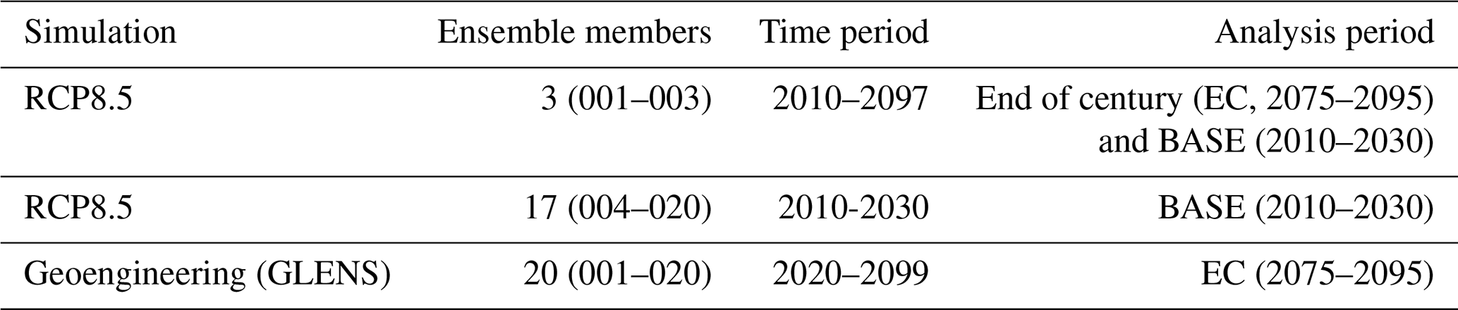
The complete GLENS dataset comprises three RCP8.5 simulations without geoengineering from 2010 to 2095 or 2099 and an additional 17 members from 2010 to 2030. Hence, there are a total of 20 simulations without geoengineering for a “control” period of 2010–2030, referred to as BASE. The 20-member SAI intervention simulations are branched from their corresponding BASE member in 2020 and are referred to here as GLENS. Results are presented for the differences between an end-of-the-century (EC) period of 2075–2095, when the differences between GLENS (EC) or RCP8.5 (EC) and RCP8.5 2010–2030 (BASE) are most readily discernible from natural variability.

We note that simulations represent geoengineering to moderate the extreme climate changes expected at the end of the century under RCP8.5, with no additional reduction in anthropogenic carbon emissions. While useful for extracting signals in a noisy climate system, deployments of geoengineering are likely to be more moderate and made in combination with other methods of addressing climate change, such as greenhouse gas emission reductions and negative emissions (Tilmes et al., 2020; MacMartin et al., 2018; Keith and Irvine, 2016; Honegger et al., 2021).

2.2 Extreme indices

A subset of the full set of ETCCDI indices (from here on referred to as ETCCDIs) is listed in Table 2 and discussed in this paper. Given the number of indices and global coverage of the analysis, only the annual ETCCDIs are discussed in this paper. However, some seasonality is implicit in indices such as the annual coldest and warmest temperatures.

Table 2 Selection of extreme indices developed by ETCCDI (Klein Tank et al., 2009). Percentiles marked with ^* were estimated from a base period of 2010–2030 and are only included in the Supplement; values are calculated as a climatological average for the end of the century (2075–2095).

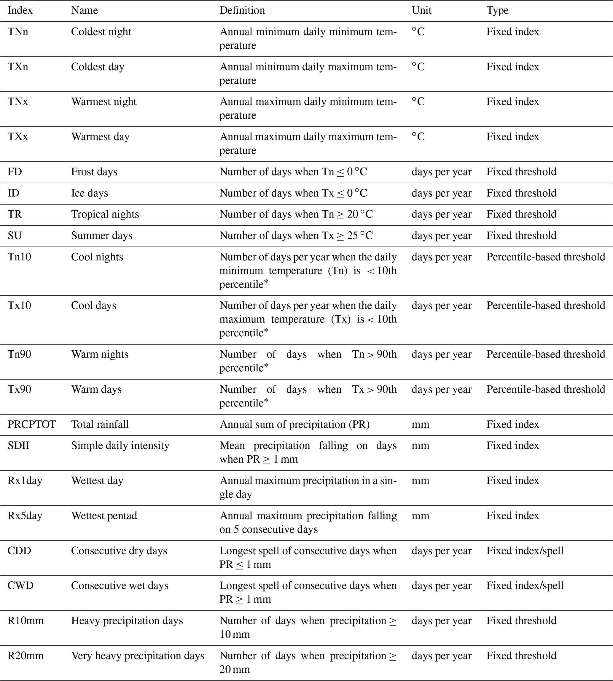
The ETCCDIs fall into three groups: fixed indices such as the annual minima and maxima and spell duration, fixed thresholds such as the annual frequency of days with >10 mm precipitation, and percentile thresholds such as the annual frequency of days with temperatures exceeding the 90th percentile. Fixed threshold indices are useful where they give a sense of the implications of changed temperatures and precipitation patterns. For instance, the number of days above zero may indicate the potential for vegetation growth. However, fixed threshold indices can be meaningless where they seldom occur and will not change (such as the number of days falling below 0 ^∘C in the Arabian Peninsula). The duration of the longest consecutive dry periods (CDD), or dry spells, serves as a simple proxy for drought conditions. Both CDD and the longest consecutive number of wet days (CWD) are calculated as the longest period in any given year in the 20-year analysis period with consecutive days of precipitation above or below 1 mm. In contrast with Silmann et al. (2013a, b) we did not allow the spell duration to extend beyond a year.

Changes in fixed threshold ETCCDIs can be critical indicators for health and environmental impacts (Mearns et al., 1984; Mitchell et al., 2016), and they tend to change more rapidly than changes in the mean (Meehl et al., 2000; Asadieh and Krakauer, 2015). While such indices are not always “extreme” in and of themselves, they have been demonstrated to be more sensitive to change (e.g., Alexander et al., 2006; Frich et al., 2002). Percentile-based ETCCDIs, including the frequency of cold or warm days and nights (TX10, TX90; TN10, TN90) and the proportional contribution of the heaviest events to the annual total precipitation (R95pTot, R99pTot), demonstrated very similar patterns as those of other ETCCDIs. For completeness they are referenced in Table 2, but for brevity the ETCCDIs that are in italic font are not shown in the main text.

To facilitate comparison with other analyses using the GLENS dataset (e.g., Simpson et al., 2019) and to provide the greatest signal-to-noise ratio, we present absolute difference anomalies in ETCCDIs between an end-of-the-century period (2075–2095; EC) for simulations with and without SO₂ injections (GLENS and RCP8.5, respectively) and the BASE (2010–2030). Regional means are calculated over the 46 land-only reference regions (Iturbide et al., 2020) produced for the Intergovernmental Panel on Climate Change Assessment Report 6 (IPCC, 2021) and illustrated in Fig. 1, with abbreviations colored by continent for ease of reference to other figures. We caution that using a control period of 2010–2030 prevents direct comparison with other projections of ETCCDIs from the CMIP5 archive (e.g., Sillmann et al., 2013b; Diffenbaugh and Giorgi, 2012).

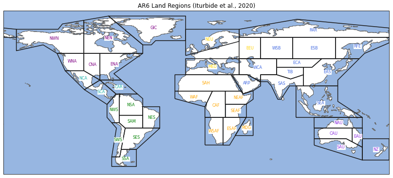
Figure 1 AR6 reference regions for land (source: Iturbide et al., 2020). Regional abbreviations are colored by continent to facilitate comparison with other figures.

Changes in precipitation patterns over land and associated changes in soil moisture are intrinsically linked to vegetation through processes like evapotranspiration, water consumption, and albedo effects (Cheng et al., 2019). Some of the ETCCDIs in Table 2 are more intuitively linked to vegetation responses than others. For instance, CDD and CWD are associated with droughts, FD and ID can be connected to growing potential, and TN90 and TX90 have important implications for heatwaves. Furthermore, the processes linking precipitation and temperature to impacts on vegetation are influenced by increasing atmospheric CO₂, which tends to increase vegetation productivity and decrease evapotranspiration (ET; Dagon and Schrag, 2016) through changes in plant water-use efficiency. In addition, the increase in diffuse radiation from SAI could also increase vegetation productivity (Xia et al., 2016). The effects of cloud cover have also been linked to differential rates of change in nighttime or daytime temperatures and the associated vegetative responses in different locations (Cox et al., 2020). These effects are explored further in Sect. 4.

3 Temperature and precipitation response

While we analyzed all of the ETCCDIs presented in Table 2, general spatial patterns of change are similar across many of them. A selection of the ETCCDIs or regions demonstrating the largest changes are presented in the following text, with additional figures included in the Supplement. The significance of the difference between GLENS EC and BASE, or RCP8.5 EC and BASE, was assessed using a two-sided Student's t test at the 5 % level.

3.1 Temperatures

3.1.1 Fixed indices

GLENS EC (2075–2095) generally projects the coldest night of the year (TNn) to be warmer across the Northern Hemisphere compared to the present climate (BASE; 2010–2030) and cooler in the Southern Hemisphere with the exception of Antarctica relative to BASE (see Figs. 2a, 3, and S1). For ease of viewing, Fig. 3 is laid out in three horizontal sections that approximately contain regions in the Americas along the zero meridian and in Asia. Also refer to Fig. 1 for color coding of regional abbreviations. The bars are composed of the regional and climatological mean TNn value for each model member, with the ensemble mean in white and full ensemble spread shown by the tails.

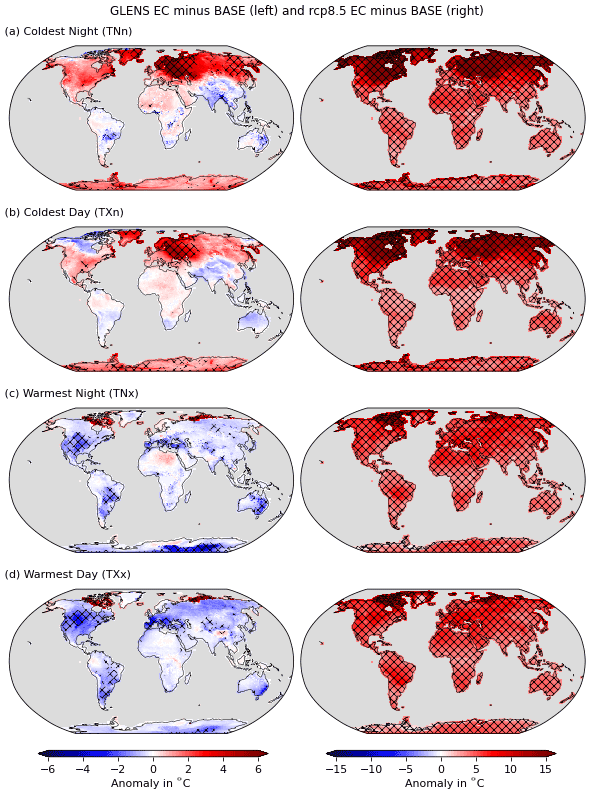
Figure 2 Projected anomalies between the GLENS EC scenario (2075–2095) and BASE (2010–2030) for the annual coldest night and day (TNn, TXn) as well as the warmest night and day (TNx, TXx) shown in the left column. Anomalies between RCP8.5 EC (2075–2095) and BASE (2010–2030) are shown in the right column. Note that the color bar is different in the right column. Hatching indicates significance at the 5 % test level using the Student's t test.

Reduction of the coldest night temperature (TNn) in GLENS EC is most noticeable across the tropics but is only of the order of 1 ^∘C and is not statistically significant. GLENS EC projects statistically significant increases in the temperature of the coldest night in central Europe by up to 8 ^∘C; this increase is around half of that projected by RCP8.5 EC. The strong winter warming in GLENS over Eurasia has been identified by others (Jiang et al., 2019; Tilmes et al., 2018) and has been linked to a strengthened Northern Hemisphere polar vortex (Banerjee et al., 2021). Similar to the coldest night, GLENS EC projects a pattern of warming for the coldest day (TXn) in the Northern Hemisphere and marginal cooling in the Southern Hemisphere, with the exception of a cooler region in the northern part of Canada (Figs. 2b, S2 and S3 in the Supplement). However, GLENS EC projects significant warming over Antarctica, with cooling in other parts of the Southern Hemisphere.

In contrast, GLENS warmest night of the year (TNx; Figs. 2c, S4 and S5 in the Supplement) projects a broad pattern of cooling across both hemispheres, with some statistically insignificant warming across the Sahara and the northern part of Canada as well as significant (albeit marginal) cooling over Eurasia. GLENS EC warmest day of the year (TXx; Figs. 2d; S6 and S7 in the Supplement) follows the same pattern of warming and cooling shown by TNx, with the greatest cooling occurring at 30–60^∘ N of around −3 ^∘C; exceptions are northern Siberia and northern Canada. The warming in very high latitudes (>80^∘ N or >80^∘ S) arises from the implementation of the Equator-to-pole temperature control in the feedback algorithm, whereby increased cooling in the high Arctic and Antarctica leads to warmer spots at slightly lower latitudes (Kravitz et al., 2017).

3.1.2 Fixed thresholds

Changes in the number of nights with a minimum below 0 ^∘C (frost days, FD; Figs. 4a, S8 and S9 in the Supplement) may reflect considerable impacts for human and ecological health. In some regions, maintaining or increasing the frequency of the coldest days could be beneficial by suppressing the growth of pests or transmission of vector- and zoonotic-borne disease (e.g., Logan et al., 2010; Mills et al., 2010). However, colder temperatures in combination with other socioeconomic factors can also increase the risk of winter mortality (Smith et al., 2014). Sillmann et al. (2013b) noted spatially consistent decreases in the projected frequency of FD across all climate models and emissions scenarios. CESM1 RCP8.5 projections were amongst the largest decreases, ranging from a global mean decrease of 30 d yr⁻¹ to over 100 d yr⁻¹ at high latitudes by the end of the century, as illustrated in the right column of Fig. 4a.

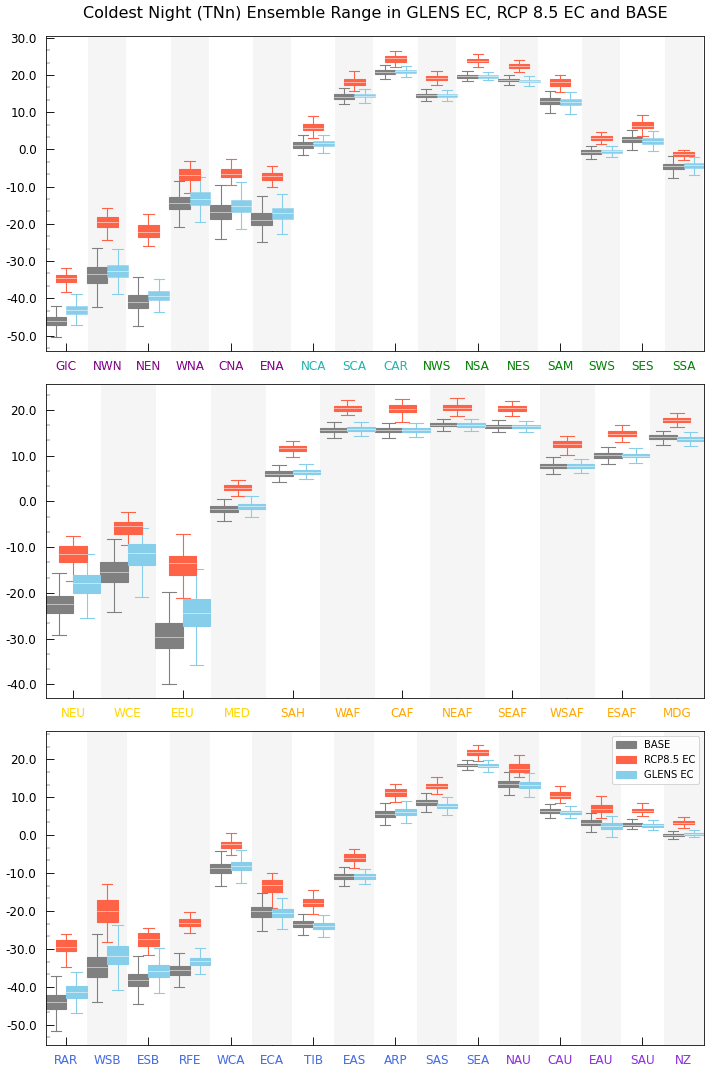
Figure 3 Climatological mean of the coldest night (TNn) for BASE (2010–2030) in gray, GLENS end of century (EC; 2075–2095) in blue, and RCP8.5 EC in red in each of the AR6 regions except Antarctica (Iturbide et al., 2020). Boxes show the ensemble mean in white with the limits set at 25 % and 75 % of the ensemble spread; whiskers denote 5 % and 95 % ensemble spread.

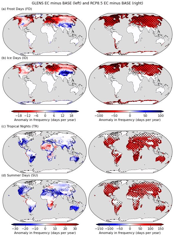
Figure 4 The same as Fig. 2, but containing projected anomalies in the frequency of daily minima <0 ^∘C (frost days, FD), daily maxima <0 ^∘C (ice days, ID), daily minima >20 ^∘C (tropical nights, TR), and daily maxima >25 ^∘C (summer days, SU). Hatching indicates significance at the 5 % test level using the Student's t test.

The pattern of GLENS EC changes in FD (Fig. 4a, left) differs in magnitude from RCP8.5 EC (Fig. 4a, right) and in some cases differs in sign, with some regions of increasing FD. Similar to projected changes in mean temperatures (Tilmes et al., 2018), GLENS EC projects cooler temperatures in the mountainous regions of Asia, with significant decreases in FD. Similarly, GLENS EC projects significant decreases in FD over northern Europe that also tally with projected changes in the frequency of cool nights (Figs. S10 and S11 in the Supplement) and increases in TNn. Projections for the frequency of daily maxima below 0 ^∘C (ice days; ID) in GLENS EC are very similar to those of FD frequency and to the projected changes in the coldest day (Fig. 2b), but they are only statistically significant across Europe (decreases) and parts of Asia (increases). Refer to Figs. 4b and S12 to S15 in the Supplement, including contextual changes in the frequency of cold days.

Nighttime low temperatures exceeding 20 ^∘C (tropical nights, TR) are a potential indicator of health-related impacts in extratropical regions (Mitchell et al., 2016) and in many locations have been observed to increase more rapidly than daytime temperatures (Cox et al., 2020). Of note is the projected increase in frequency in TR over the Middle East and North Africa region in GLENS EC (Figs. 4c; S16 and S17 in the Supplement) similar to the projected increase in TNx (Fig. 2c) but where other ETCCDIs, including warm nights (Figs. S18 and S19 in the Supplement), project little change in temperature. These increases are lower than those projected by RCP8.5 EC (Fig. 4c, right). In a pattern noted above, the frequency of daytime temperatures exceeding 25 ^∘C (summer days, SU) generally decreases, particularly in the tropics (Figs. 4d; S20 and S21 in the Supplement). The main exception to this pattern is southern Africa where increases in SU up to 20 d are projected in GLENS EC. Localized patterns of warming and cooling have also been linked to changes in cloud cover, humidity, and vegetative responses (Cox et al., 2020; Visioni et al., 2020). Prior research has indicated that medium-altitude clouds, which can have impacts on localized temperature differences, are more sensitive to the presence of sulfate aerosols than to climate-related warming (Visioni et al., 2021). However, these cloud effects were not explicitly examined in this research. While GLENS EC projects increases in SU, the increases are still substantially lower than those projected by RCP8.5 EC (Fig. 4d, right) and match the pattern of limited changes in daytime temperatures when compared to TXx and the frequency of hot days (Figs. S22 and S23 in the Supplement).

3.1.3 Temperature summary

While the changes in GLENS EC ETCCDIs for temperature generally reflect the same spatial patterns as those reported for mean temperature (Tilmes et al., 2018; Cheng et al., 2022), there are some notable differences. Figure 5 compares the GLENS EC projected changes in mean temperature, in the center, against projected changes in the warmest night (TNx) for selected regions. In all cases, the time series are dominated by the increases in TNx for RCP8.5 EC. However, where large increases in the mean are projected over Europe in GLENS EC, decreases are projected in TNx; in contrast, no change in the mean over northeastern North America is partnered by an increase in TNx. Climate change projections demonstrate that daily minimum temperatures (i.e., the nighttime low) often increase more rapidly than mean temperatures. While many increases are offset within GLENS EC, there are significant increases in the coldest night of the year (TNn) and a decreased frequency of frost and ice days (FD, ID), in conjunction with the reported winter warming over Eurasia (Banerjee et al., 2021). GLENS EC also projects increases in the frequency of tropical nights (TR) over much of Africa and parts of Central America, although these are lower than the increases projected in RCP8.5 EC. The projected increase in annual maximum temperature (TXx) over the Tibetan Plateau in GLENS EC is an interesting contrast to the projected cooling in this region but is consistent with other research (Muthalya et al., 2018b; Irvine et al., 2019). However, the change is not apparent in regional means due to the projected decrease in surrounding temperatures. As discussed below, the warming over the Tibetan Plateau and northern India is linked to changes in monsoonal rain (Visioni et al., 2020).

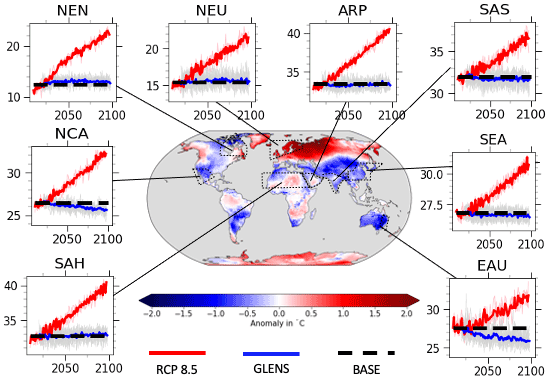
Figure 5 Ensemble mean of projected changes in mean global temperature for GLENS EC (2075–2095) minus BASE (2010–2030) with inset regional time series of the warmest night (TNx) for northeastern North America (NEN), northern Central America (NCA), Sahara (SAH), northern Europe (NEU), Arabian Peninsula (ARP), South Asia (SAS), East Asia (EAS), and eastern Australia (EAU). Regional time series comprise ensemble mean TNx for GLENS EC minus BASE in thick blue and individual members in light gray, ensemble mean TNx for RCP8.5 EC in thick red and individual members in light pink, and ensemble and climatological mean TNx for BASE in thick dashed black.

We note that many of the projected increases in temperature extremes in GLENS EC are not statistically significant with respect to the current climate (BASE). This is a positive result demonstrating that the mean climate state has been maintained at the nominal BASE climate in this set of simulations. However, these simulations represent only one snapshot of the potential response to SAI; other simulations that commence at a different time period or use different feedback controls may show other results. Furthermore, changes in the hydrological cycle and vegetative responses may be very different from changes in temperature, as discussed in Sects. 3.2 and 4.

3.2 Precipitation

Considerable variation in precipitation patterns tends to overwhelm any emergent climate signal, such that many of the changes discussed below are not statistically significant. Even though we are examining end-of-the-century changes (2075–2095), the differences are often not distinguishable from variability until approximately the second half of the climate period (i.e., 2085–2095).

3.2.1 Fixed indices

GLENS EC (2075–2095) global mean precipitation over land is projected to change very little with respect to BASE (2010–2030; Cheng et al., 2019; Simpson et al., 2019). However, there are spatial variations in this pattern that relate to orographic and oceanic processes, in addition to seasonal variations. For example, Simpson et al. (2019) reported a decrease in annual total precipitation (PRCPTOT) in regions where the mean daily precipitation ≥5 mm d⁻¹, with reductions over land affecting India, Indonesia, and northeastern South America as well as increases over central Australia. As with temperatures, a strong seasonal signal is apparent that affects the intensity of GLENS EC projected increases and decreases. The patterns of change in GLENS EC annual mean precipitation are accentuated during the Northern Hemisphere summer (JJA) and linked to a reduction in the east–west gradient of Pacific sea surface temperatures (SSTs) (Simpson et al., 2019). In contrast, those same regions are projected to experience little to no change during the Northern Hemisphere winter (DJF), while Indonesia and the northern territories of Australia are projected to experience increased precipitation. Again, this is linked to changes in the east–west gradient of Pacific SSTs (Simpson et al., 2019; Trisos et al., 2018).

GLENS EC projected changes in PRCPTOT (Figs. 6a; S24 and S25 in the Supplement) relative to BASE show little spatial change except in the tropics, and in general few of those changes are statistically significant. One of the few regions to project significant change in PRCPTOT is the coastal part of West Africa, where the decreases are on the order of 300 mm yr⁻¹. Another region with localized projected increases in PRCPTOT is the La Plata basin in southeastern South America, where increases are also projected in river discharge (Camilloni et al., 2022). Other regions project increases and decreases that replicate the general pattern of “wet gets drier, dry gets wetter” reported by Simpson et al. (2019), with considerable year-to-year variability. Haywood et al. (2013) reported a contraction in the Intertropical Convergence Zone (ITCZ) in geoengineering simulations that corresponds to the projected changes in annual moisture patterns. By design, the GLENS simulations aim to minimize changes to the ITCZ. However, recent evaluations have concluded that there is a very slight southward shift even when interhemispheric temperature gradients are maintained (Lee et al., 2020; Alamou et al., 2022; Cheng et al., 2019). This is also accompanied by a weakening (of the order of 10 %) of the Hadley cell intensity (Cheng et al., 2022). The simple daily intensity, or mean wet day total (SDII; Figs. 6b, S26 and S27 in the Supplement), starts to illustrate that the projected increases and decreases in PRCPTOT in GLENS EC arise from a change in the number of days with precipitation, not only the intensity on those days. For instance, parts of Western Australia, the MENA, and southern China project increases in SDII in GLENS EC where little or no change is projected in PRCPTOT.

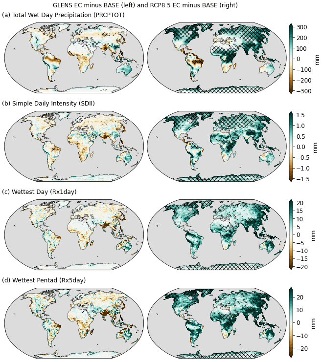
Figure 6 Similar to Fig. 2, but for projected changes in (a) annual precipitation (PRCPTOT), (b) the mean wet day volume (SDII), (c) annual maximum precipitation (Rx1day), and (d) annual wettest pentad (Rx5day). Hatching indicates significance at the 5 % test level using the Student's t test.

The greatest projected decreases in annual total precipitation within the ITCZ are, with the exception of the Indian monsoon region, projected to have little or no change in the annual wettest day (Rx1day; Figs. 6c, S28 and S29 in the Supplement) and wettest pentad (Rx5day; Figs. 6d, S30 and S31 in the Supplement). In contrast, RCP8.5 EC projects significant increases in PRCPTOT across much of the globe that are largely driven by increases in the most intense few events per year (Fig. 6, right). Under the RCP8.5 EC scenario there is projected to be greater volatility in the distribution of days with precipitation such that even regions that are projected to dry will also experience more intense extreme events (e.g., northern South America). This contrasts with GLENS EC for which changes in PRCPTOT and the most extreme events appear to move in the same direction (i.e., decreases in Rx1day, and lower PRCPTOT), leading to a more uniform distribution of precipitation.

The most striking change in GLENS EC is the projected drying over the northern part of India and Bangladesh, with changes in all extreme precipitation ETCCDIs. GLENS EC projects decreases in annual maxima over northern India (Fig. 6c) that are approximately co-located with projected cooling compared to BASE (e.g., Fig. 5), thus following the direction of change expected with changes in atmospheric moisture content. The related decreases in soil moisture and latent heat flux over northern India in GLENS are discussed further in Sect. 4.3. This has been linked to the seasonality of temperature changes over the Tibetan Plateau in response to annual rather than seasonal injection strategies, resulting in changes in the monsoon precipitation (Visioni et al., 2020).

3.2.2 Spells

Regions with projected decreases in PRCPTOT under RCP8.5 EC tend to project increases in the duration of the longest dry spells (CDD) and decreases in the duration of wet spells (CWD; Sillmann et al., 2013b; Giorgi et al., 2014), as shown in Fig. 7 (right column). However, GLENS EC projections of CDD (Figs. 7a; S32 and S33 in the Supplement) and CWD (Figs. 7b; S34 and S35 in the Supplement) are more complicated, with lower apparent correlation between changes in the longest dry and wet spells and changes in PRCPTOT. Given that other metrics (SDII, Rx1Day, R10mm) indicate that changes in frequency and intensity affect PRCPTOT, this suggests that dry day persistence decreases in GLENS EC in contrast with the increases found for non-SAI projections (Giorgi et al., 2019). Furthermore, increases or decreases in the longest dry spell do not necessarily correspond to changes in the longest wet spell (CWD). Projected decreases in the longest dry spell over the Sahara and Middle East (SAR, EAP) in GLENS EC are considerable but not statistically significant, and as noted by Pinto et al. (2020) these are accompanied by increases in the southeast (SEAF, ESAF) and highlight the dichotomy of regions that benefit from, or are further disadvantaged by, SAI. Furthermore, the projected changes in GLENS EC are spatially variable and may only become more understandable with a regional analysis (e.g., Camilloni et al., 2022)

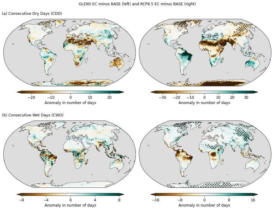
Figure 7 Similar to Fig. 2, but for projected changes in (a) the longest spell of dry days (CDD) and (b) longest spell of wet days (CWD). Hatching indicates significance at the 5 % test level using the Student's t test.

3.2.3 Fixed thresholds

Projected changes in GLENS EC and RCP8.5 EC in the frequency of heavy (R10mm) and very heavy (R20mm) precipitation days are shown in Fig. 8 (and Figs. S36–S39 in the Supplement). Within the ITCZ, where SDII is near 10 mm d⁻¹, the pattern of projected changes in GLENS EC (Fig. 8, left) is very similar to that of other metrics and indicates that the changes are proportional across the precipitation intensity distribution. Outside the ITCZ, GLENS EC projects a less disproportional shift than projected by RCP8.5 EC. That is, wet regions may become wetter, but not as a result of precipitation falling in fewer more intense events. Thus, regions such as northeastern South America and northeastern India that have considerable projected decreases in PRCPTOT under GLENS EC also have projected decreases in the number of R10mm and R20mm days, but not in the duration of the longest dry spells. Similarly, the GLENS EC projected increase in PRCPTOT over Indonesia is related to projected increases in heavy precipitation days and not to the intensity of the most extreme events (Rx1day, Rx5day). The projected decreases in R10mm and R20mm over South America and central Africa also correspond to regions of projected decreases in the annual maximum temperatures (TNx, TXx; Fig. 2), as anticipated under the Clausius–Clapeyron relationship.

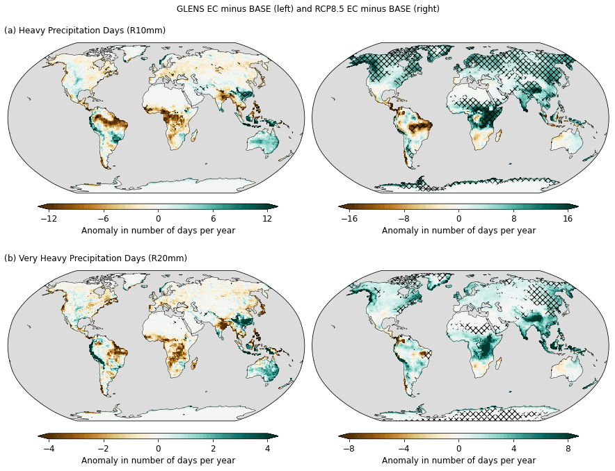
Figure 8 Similar to Fig. 2, but for projected changes in (a) the frequency of days with heavy precipitation (R10mm) and (b) days with very heavy precipitation (R20mm). Hatching indicates significance at the 5 % test level using the Student's t test.

3.2.4 Precipitation summary

As with temperature, patterns for the precipitation ETCCDIs are very similar to those seen in GLENS EC mean precipitation (Simpson et al., 2019), but the changes are not uniform across all indices or all locations. Figure 9 illustrates the change in mean precipitation between GLENS EC and BASE (Simpson et al., 2019) together with projected changes in the frequency of heavy rain days (R10mm) for several regions. While GLENS EC generally projects increases in precipitation while RCP8.5 EC projects decreases and vice versa, there are some exceptions to this pattern. In particular, some parts of South America and Africa are projected to experience enhanced drying compared to BASE under both GLENS EC and RCP8.5 EC (Cheng et al., 2019; Simpson et al., 2019; Pinto et al., 2020), and this is discussed further in the context of vegetative responses in Sect. 4. However, we find that many of the projected changes in GLENS EC are not statistically significant when compared to the current climate.

GLENS EC changes in PRCPTOT are related in part to changes in the intensity on the wettest days, but also to the frequency of days with precipitation. For instance, the greatest projected decreases in PRCPTOT within the ITCZ are accompanied by projected decreases in the number of days with more than 10 mm of precipitation (R10mm; Fig. 8a). That is, there is a shift towards more days with less intense rain and fewer very intense rain days, consistent with other experiments (Ji et al., 2018; Camilloni et al., 2022). Changes in the heavier events also follow the direction of change expected from changes in atmospheric moisture capacity, with changes in Rx1day largely corresponding to changes in daytime temperature such as decreases over northern South America (Fig. 5).

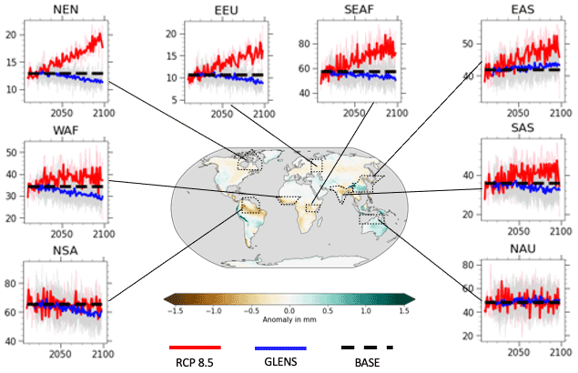
Figure 9 Ensemble mean of projected changes in mean daily precipitation for GLENS EC (2075–2095) minus BASE (2010–2030) with inset regional time series of frequency of days >10 mm (R10mm) for northeastern North America (NEN), northern South America (NSA), southeastern Africa (SES), western Africa (WAF), eastern Europe (EEU), South Asia (SAS), East Asia (EAS), and northern Australia (NAU). Regional time series comprise ensemble mean R10mm for GLENS EC minus BASE in thick blue and individual members in light gray, ensemble mean R10mm for RCP8.5 EC in thick red and individual members in light pink, and ensemble and climatological mean R10mm for BASE in thick dashed black.

4 Vegetation response

Relative to BASE, GLENS EC shows a mix of increases and decreases in latent heat flux (LHF; Fig. 10a), a mix of increases and decreases in soil moisture at the surface (SM10; Fig. 10b), and consistent increases in both leaf area index (LAI; Fig. 10c) and gross primary production (GPP; Fig. 10d). Examining the partitioning of evaporative fluxes shows mixed responses in GLENS EC relative to BASE, with changes in ground evaporation (Fig. 11a) and transpiration (Fig. 11c) generally following the sign of the changes in LHF and canopy evaporation generally increasing (Fig. 11b). When comparing these changes with the changes in RCP8.5 EC relative to BASE (center columns of Figs. 10 and 11), the vegetation changes in GLENS (left columns of Figs. 10 and 11) are generally more muted. LHF (Fig. 10a), ground evaporation (Fig. 11a), and transpiration (Fig. 11c) largely increase under RCP8.5, contrasting with smaller-magnitude decreases seen with GLENS.

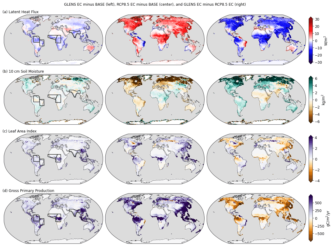
Figure 10 Projected changes between GLENS EC (2075–2095) and BASE (2010–2030) in the left column, changes between RCP8.5 EC (2075–2095) and BASE (2010–2030) in the center column, and changes between GLENS EC (2075–2095) and RCP8.5 EC (2075–2095) in the right column for (a) latent heat flux, (b) soil moisture in the top 10 cm, (c) total leaf area index, and (d) gross primary production. Black polygons in the left column highlight the following regions: northeastern South America (NSA), northern South America, western Africa (WAF), central Africa (CAF), and South Asia (SAS).

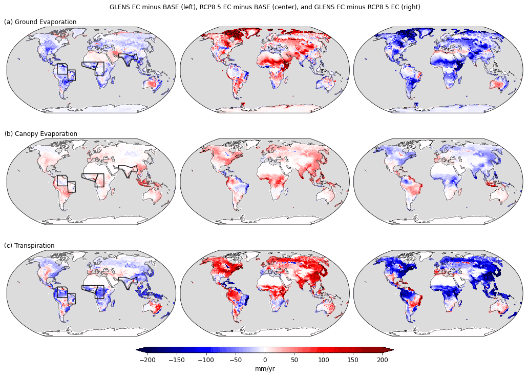
Figure 11 Projected changes between GLENS EC (2075–2095) and BASE (2010–2030) in the left column, changes between RCP8.5 EC (2075–2095) and BASE (2010–2030) in the center column, and changes between GLENS EC (2075–2095) and RCP8.5 EC (2075–2095) in the right column in (a) ground evaporation, (b) canopy evaporation, and (c) transpiration. Highlighted regions in the left column are as for Fig. 10.

Both comparisons are relative to BASE, so further examining the changes in GLENS EC relative to RCP8.5 EC (right columns of Figs. 10 and 11) reveals stronger-magnitude decreases in LHF and ground evaporation (likely due to decreases in solar radiation limiting the energy available for evaporation) and associated increases in SM10. This comparison shows that the overall GLENS EC responses are a combination of increases in LHF and ground evaporation as well as decreases in SM10 from unmitigated climate change, which are countered by larger-magnitude decreases in LHF and ground evaporation as well as increases in SM10 from changes in solar radiation. LAI (Fig. 10c) and GPP (Fig. 10d) increase at a larger magnitude under RCP8.5 EC minus BASE relative to GLENS EC minus BASE. In contrast, the changes in GLENS EC relative to RCP8.5 EC show large areas of decrease in LAI and GPP. This comparison does not include any change in CO₂, so the changes in solar radiation are isolated from the associated greenhouse warming under GLENS EC relative to RCP8.5 EC. Looking across all the columns of Fig. 10 shows that the overall GLENS EC increases in LAI and GPP largely come from CO₂ fertilization, which is countered by the decreases in LAI and GPP (and associated decreases in transpiration) from changes in solar radiation. Changes in solar radiation would likely impact vegetation through several pathways: (1) decreasing temperatures, which could inhibit growth (Dagon and Schrag, 2016), (2) increasing the fraction of diffuse radiation and thus potentially increasing photosynthesis (Xia et al., 2016), and (3) changing the availability of soil moisture locally, which could impact water fluxes at the surface and thus productivity (Cheng et al., 2019).

In this section, we focus on three regions where the GLENS EC vegetation responses and associated mechanisms are different, despite similarities in the projected temperature and precipitation. These regions further emphasize that despite the ability to maintain global mean temperature and precipitation at a target level, the effects of climate change cannot be completely offset and will have regional and temporal differences that could be considerable (Jones et al., 2018; Simpson et al., 2019; Tilmes et al., 2013). The three regions of interest are northern and northeastern South America, western and central Africa, and India (South Asia in AR6 regions), and they are marked in the first columns of Figs. 10 and 11. All of these regions have been highlighted as sensitive to the effects of changes in the hydrological cycle under SAI (Bhowmick et al., 2021; Camilloni et al., 2022; Da-Allada et al., 2020; Jones et al., 2018; Pinto et al., 2020; Simpson et al., 2019). Relative to BASE, GLENS EC projects decreases in LHF (Fig. 10a), together with increases in LAI (Fig. 10c) and GPP (Fig. 10d) in all three regions, but with different partitioning of the evaporative fluxes (Fig. 11) related to changes in soil moisture at the surface (Fig. 10b) and local changes in temperature and precipitation.

4.1 North and northeastern South America

The Amazon basin is projected to dry considerably under unmitigated climate change, with changes in evapotranspiration playing a large part in the hydrological cycle changes (Halladay and Good, 2017). Other research has also indicated that SAI may offset some of the projected drying but not the full effects (Cheng et al., 2019; Simpson et al., 2019), with plant feedbacks identified as the main contributing factor (Jones et al., 2018; Xia et al., 2016).

The GLENS projected decreases in mean precipitation occur across the full distribution of precipitation, with resultant decreases in soil moisture under GLENS EC relative to BASE in these regions (Fig. 10b). These decreases are accompanied by different rates of change in the daytime (TX) and nighttime (TN) temperatures with marginal increases in the coldest day TXn but decreases in the warmest day (TXx) and warmest night (TNx; see Figs. 2, 5, and 12). However, the projected changes in all metrics under GLENS EC are not statistically significant and well within the ensemble range of the BASE climate. Changes in all three metrics correlate with the posited relationship between cloud cover, vegetation, and precipitation, whereby more rapid nighttime warming is associated with decreased cloud cover and vice versa (Cox et al., 2020), and these reflect the potential for increases in cloud cover (Krishnamohan and Bala, 2022; Visioni et al., 2021). The projected change in water flux partitioning appears to be linked to the change in the persistence of wet and dry periods. That is, increases in vegetation LAI along with increases in atmospheric CO₂ and decreases in solar radiation under GLENS EC relative to BASE lead to more efficient water recycling, with less ground evaporation (Fig. 11a) and transpiration (Fig. 11c) but more canopy evaporation in parts of the region (Fig. 11b), coupled with lower atmospheric moisture content and shorter wet spells (CWD, Fig. 13). Figure 14 also illustrates that there is considerable year-to-year variability in projected precipitation but that overall mean daily precipitation (SDII) under GLENS EC fluctuates around the climatological mean SDII for both NSA and NES. Under RCP8.5 EC relative to BASE, the decreases in soil moisture in these regions are larger than in GLENS EC (Fig. 10b), along with stronger decreases in LHF (Fig. 10a). Thus, the greater increases in temperature extremes under RCP8.5 EC relative to BASE across all metrics (Fig. 12) could partially be due to a lack of evaporative cooling. Comparing GLENS EC relative to RCP8.5 EC in these regions shows that decreases in solar radiation lead to increases in soil moisture (Fig. 10b), coupled with longer wet spells (Fig. 13), which act to counter the drying from unmitigated climate change.

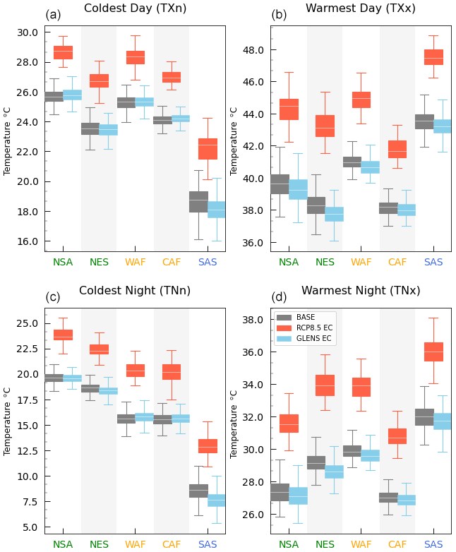
Figure 12 Regional box plots indicating the ensemble ranges of temperature indices for BASE (2010–2030; gray boxes), RCP8.5 EC (2075–2095; red boxes), and GLENS EC (2075–2095; blue boxes) for the annual minimum daily maximum (coldest day, TXn, a), annual maximum daily maximum (warmest day, TXx, b), annual minimum daily minimum (coldest night, TNn, c), and annual maximum daily minimum (warmest night, TNx, d) for northern South America (NSA), northeastern South America (NES), western Africa (WAF), central Africa (CAF), and South Asia (SAS).

Figure 13 Regional box plots indicating the ensemble ranges of temperature indices for BASE (2010–2030; gray boxes), RCP8.5 EC (2075–2095; red boxes), and GLENS EC (2075–2095; blue boxes) for the annual maximum daily precipitation (wettest day, Rx1day, a), number of heavy rain days per year (R10mm, b), longest consecutive spell of wet days per year (longest wet spell, CWD, c), and longest consecutive spell of dry days per year (longest dry spell, CDD, d) for the same regions as Fig. 12.

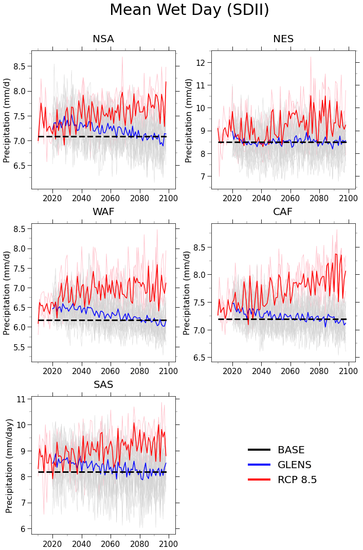
Figure 14 Time series indicating the ensemble ranges of temperature indices for BASE (2010–2030; black line), RCP8.5 (2010–2095; red lines), and GLENS (2020–2095; blue line) for the mean wet day precipitation (SDII) for the same regions as Fig. 12.

4.2 Western and central Africa

RCP8.5 EC precipitation patterns over the Sahel as well as central and western Africa are likely to be more extremely distributed, with increased intensity of the wettest days, shorter dry spells, and shorter wet spells. Similar to the Amazon basin, GLENS EC appears to offset some of the extremes in temperature and precipitation projected by RCP8.5 EC over the Sahel but would likely lead to decreases in precipitation over western Africa and southern Africa (Da-Allada et al., 2020; Pinto et al., 2020), as seen in the changes in SDII for WAF and CAF (Fig. 14). The increases in LAI and GPP (Fig. 10c, d) in GLENS EC relative to BASE in these regions are accompanied by decreases in LHF (Fig. 10a) and very marginal decreases in the most extreme daily temperatures (Fig. 12), with some warmer summer days (SU) and cooler tropical nights (TR) at the edges of this domain (Fig. 4) but decreases in mean and extreme precipitation (Figs. 13 and 14). This largely follows the anticipated asymmetric diel warming relationships whereby more rapid warming in nighttime minima than daytime maxima is attributed to reduced cloud cover (Cox et al., 2020; Krishnamohan and Bala, 2022; Visioni et al., 2021) together with increased persistence of dry spells (Pinto et al., 2020). As with other locations in the tropics, the decreases in LHF are also driven primarily by decreases in transpiration (Fig. 11c; Dagon and Schrag, 2019). Combined with projected decreases in precipitation, ground evaporation is also projected to decrease (Fig. 11a) and soil moisture to remain unchanged (Fig. 10b) in GLENS EC relative to BASE, pointing to the complexity of the hydrological cycle and the importance of assessing many different metrics for the full potential impact of SAI over any region. Under RCP8.5 EC relative to BASE in these regions, LHF increases (Fig. 10a), driven by increases in all three evaporative fluxes (Fig. 11), along with increases in LAI (Fig. 10c) and GPP (Fig. 10d) due to the CO₂ fertilization effect. This is in contrast to the decreases in evaporative fluxes, LAI, and GPP seen in these regions under GLENS EC relative to RCP8.5 EC, driven by the decreases in solar radiation. The evaporative flux decreases from less sunlight are larger than the associated increases from unmitigated warming, leading to overall decreases in LHF under GLENS EC relative to BASE in these regions. The opposite is true for LAI and GPP, for which the increases from unmitigated warming and increased CO₂ are larger than the decreases from less sunlight, leading to overall increases in LAI and GPP under GLENS EC relative to BASE.

4.3 India (South Asia)

The regional reductions in extreme precipitation metrics under GLENS EC relative to BASE (Figs. 13 and 14), i.e., drying, over India are confirmed by examining changes in latent heat flux and soil moisture (Fig. 10a, b). Away from the tropics, LHF is dominated by ground evaporation and soil moisture, both of which decrease in the GLENS EC projections relative to BASE. The reduction in LHF is also likely linked to reductions in cloud cover (Krishnamohan and Bala, 2022; Visioni et al., 2021). However, there is little change in LAI or canopy evaporation, coupled with a slight increase in the asymmetry of the rate of decrease in TX versus TN in GLENS EC (refer to Sect. 3.1 and Figs. 2, 5, and 12). The changes in all precipitation ETCCDIs over India are most closely related to the changes in mean JJA precipitation and hence the summer monsoon, with variability in the ITCZ and differential temperature gradients over the Tibetan Plateau playing a large role (Bhowmic et al., 2021; Visioni et al., 2020). Again, Figs. 13 and 14 highlight the temporal variability in the precipitation metrics, together with the spread of the model ensemble. Examining the breakdown of hydrologic responses in this region from changes in CO₂ versus changes in solar radiation follows what is seen previously, with changes in solar radiation dominating the overall changes in LHF and soil moisture leading to decreases under GLENS EC relative to BASE.

4.4 Vegetation summary

The contrast in vegetative responses in these three regions emphasizes the fact that several different mechanisms can be responsible for regional drying under SAI (Fig. 9). Jones et al. (2018) hypothesized three principal mechanisms that relate to changes in the hydrological cycle: an increased tendency for the ITCZ to favor the warmer hemisphere (India), changes in SST over the Atlantic and western Pacific that mimic an El Niño-like response (western and central Africa), or plant physiological responses (northern and northeastern South America). Similar to Jones et al. (2018), our results show that the main driver of Amazon drying, and likely other highly vegetated regions in the tropics, is the response of vegetation to the combination of increased CO₂ and decreased solar radiation, leading to more efficient water use and cloud development. Drying over central and western Africa reflects a combination of diel asymmetry in warming with reduced cloud coverage and decreased evaporative fluxes, which are likely influenced by changes in SST. Over India the contrast between day and night temperatures also acts to decrease cloud cover, with accompanying decreases in precipitation and soil moisture but little to no change in vegetation LAI. This suggests that drying over India is more closely related to the temperature gradients influenced by the equatorward shift of water-transporting systems than specific changes in vegetative behavior. All three regions show that decreases in solar radiation from SAI often lead to changes in the opposite direction from the projected changes from unmitigated climate warming and increased CO₂ and that the overall regional vegetation response in GLENS EC relative to BASE is a complex combination of these two factors.

5 Conclusions

SAI has been suggested as a possible mechanism to moderate some of the effects of climate change while more long-term and robust strategies to phase out anthropogenic carbon emissions take effect (Keith and Irvine, 2016; MacMartin et al., 2018; Tilmes et al., 2020; Honegger et al., 2021). It is also widely acknowledged that such a measure will bring benefits and disadvantages, thus necessitating a proper assessment of the different trade-offs and risks (Kravitz et al., 2021; Florin, 2021). To contribute to that discussion, we presented an assessment of the anticipated changes to temperature and precipitation ETCCDIs, as well as associated vegetation responses, under a geoengineering scenario intended to moderate the extreme climatic changes expected under RCP8.5. This ensemble explicitly simulates the responses from aerosols and offers the opportunity to determine whether the responses are distinguishable from internal variability.

We find that GLENS is generally successful at maintaining mean temperature and mean precipitation near 2020 levels. Where GLENS EC either does not offset or is too aggressive in compensating for projected changes in ETCCDIs under RCP8.5 EC, the changes are similar to those reported for mean temperature and mean precipitation (Tilmes et al., 2018; Simpson et al., 2019; Cheng et al., 2022). Furthermore, many of the projected changes in ETCCDIs in GLENS EC are not significantly different from the simulated current climate (BASE), indicating that SAI could offset the worst effects projected by RCP8.5 EC. However, we also note that SAI is preferentially more effective for daytime temperatures than nighttime due to the reduction in incoming solar irradiation, resulting in warmer minimum temperatures and cooler maximum temperatures (Curry et al., 2014; Malik et al., 2020). In addition to the winter warming over Europe, North America, and Asia (Banerjee et al., 2021), our results indicate asymmetric increases in nighttime temperatures (TNn, TR) compared to cooler days in the summer (TXx, SU). GLENS EC projects increases in warm nights over northern India, which contrast with the projected cooling in mean temperatures (Tilmes et al., 2018) and in extreme temperatures in the surrounding region (TNx, TXx) but are consistent with other research (Muthalya et al., 2018b; Irvine et al., 2019) and are likely driven by seasonal variations in the ocean–land temperature contrasts (Visioni et al., 2020; Krishnamohan and Bala, 2022). Furthermore, the projected amplitude of changes is greater at higher latitudes even though the changes scale with global mean temperatures (Kharin et al., 2018).

The asymmetry of changes in warm and cool events has been linked to a contraction or shift in the Intertropical Convergence Zone (ITCZ) in other geoengineering simulations (Haywood et al., 2013; Krishnamohan and Bala, 2022). By design, the GLENS simulations aim to minimize changes to the ITCZ. However, recent evaluations have concluded that there is a very slight southward shift even when interhemispheric temperature gradients are maintained (Lee et al., 2020; Alamou et al., 2020; Cheng et al., 2019). This is also accompanied by a weakening (of the order of 10 %) of the Hadley cell intensity (Cheng et al., 2022). Changes in the frequency and strength of El Niño and La Niña events as a result of SAI are difficult to confirm (Gabriel and Robock, 2015). However, GLENS EC projected equatorward shifts in westerlies and storm tracks (Karami et al., 2020), together with increasing precipitation over Australia and weakening of the African and Indian monsoons (Da-Allada et al., 2020; Bhowmick et al., 2021), support a weakened ENSO signal compared to present day (Malik et al., 2020). In keeping with these results, we find that projected changes in the annual total precipitation in GLENS arise from a change in the number of days with precipitation, not only the intensity on those days. Thus, GLENS EC projects precipitation on more days with fewer very intense events.

Vegetation responses are very sensitive to changes in precipitation and temperature. In particular, contrasting rates of change in day and night temperatures play a large role in the development of clouds and vegetation responses (Cox et al., 2020). We find that GLENS EC projected increases in leaf area index and gross primary production within the tropics (e.g., the Amazon) are associated with decreases in temperature and precipitation extremes. These also correspond to reductions in latent heat flux (LHF) that are dominated by the decreases in transpiration as a result of increased vegetation water-use efficiency (Dagon and Schrag, 2019). However, in regions where the changes in LHF are dominated by soil moisture and ground evaporation (e.g., India), the projected drying is accompanied by little change in vegetation and is likely a response to changes in ocean–land temperature contrasts (Visioni et al., 2020; Krishnamohan and Bala, 2022). A similarly complicated picture of drying over central and western Africa relates to the GLENS projected reductions in cloud cover, asymmetric warming, and changes in evaporative fluxes compared to present-day conditions. While we did not examine it explicitly, the integrated responses of diurnal temperatures, precipitation, and vegetative responses are likely the explanation for spatially inconsistent changes in soil moisture and evapotranspiration (Cheng et al., 2019) and will be the focus of future study.

It is important to note that the GLENS simulations evaluated here represent only one snapshot of the potential response to SAI. Other simulations that commence at a different time period, employ other Earth system models, or use different feedback controls may show contrasting results in both the mean and extremes of temperature and precipitation (e.g., Richter et al., 2022). Furthermore, the differing vegetative responses between three regions reporting similar changes in precipitation extremes highlight the complexity of the hydrological cycle, especially under simultaneous changes in solar radiation and CO₂. This emphasizes the importance of assessing more than hydrometeorological metrics to understand the full impacts of both climate change and SAI scenarios.