Present and future European heat wave magnitudes: climatologies, trends, and their associated uncertainties in GCM-RCM model chains

This study investigates present and future European heat wave magnitudes, represented by the Heat Wave Magnitude Index-daily (HWMId), for regional climate models (RCMs) and the driving global climate models (GCMs) over Europe. A subset of the large EURO-CORDEX ensemble is employed to study sources of uncertainties related to the choice of GCMs, RCMs, and their combinations.

We initially compare the evaluation runs of the RCMs driven by ERA-interim reanalysis to E-OBS (observation-based estimates), finding that the RCMs can capture most of the observed spatial and temporal features of HWMId. With their higher resolution compared to GCMs, RCMs can reveal spatial features of HWMId associated with small-scale processes (e.g., orographic effects); moreover, RCMs represent large-scale features of HWMId satisfactorily (e.g., by reproducing the general pattern revealed by E-OBS with high values at western coastal regions and low values at the eastern part). Our results indicate a clear added value of the RCMs compared to the driving GCMs. Forced with the emission scenario RCP8.5, all the GCM and RCM simulations consistently project a rise in HWMId at an exponential rate. However, the climate change signals projected by the GCMs are generally attenuated when downscaled by the RCMs, with the spatial pattern also altered.

The uncertainty in a simulated future change of heat wave magnitudes following global warming can be attributed almost equally to the difference in model physics (as represented by different RCMs) and to the driving data associated with different GCMs. Regarding the uncertainty associated with RCM choice, a major factor is the different representation of the orographic effects. No consistent spatial pattern in the ensemble spread associated with different GCMs is observed between the RCMs, suggesting GCM uncertainties are transformed by RCMs in a complex manner due to the nonlinear nature of model dynamics and physics.

In summary, our results support the use of dynamical downscaling for deriving regional climate realization regarding heat wave magnitudes.

1 Introduction

Heat waves can have adverse effects on health and have been reported to lead to excessive mortality rates among people in many regions of the world (Guo et al., 2017). In Europe, the heat waves in summer 2003 (Robine et al., 2008) and 2010 (Barriopedro et al., 2011) are prominent examples. Even in high-latitude areas, such as Scandinavia, heat waves can lead to excess mortality as reported by Åström et al. (2019) for the long and warm Scandinavian summer 2018 (Wilcke et al., 2020). In addition to health problems atmospheric heat waves are often related to water shortages, a decline in agricultural production, and increased risk of forest fires or dieback, all of which can have severe impacts both on natural ecosystems and human society (IPCC, 2014).

The Intergovernmental Panel on Climate Change (IPCC) concluded that the frequency and duration of heat wave lengths have increased in the observed past on a global scale (IPCC, 2018; Seneviratne et al., 2021). Part of the observed changes in frequency and intensity of daily temperature extremes on the global scale since the mid-twentieth century has been attributed to increasing anthropogenic forcing of the climate system. Furthermore, projections for the future under scenarios of increasing greenhouse gas forcing indicate a continued increase in both intensity and duration of heat waves (Molina et al., 2020). To alleviate future problems, adaptive measures are needed, even under scenarios with strong mitigation (IPCC, 2022). Climate change adaptation, in turn, requires relevant information about changes both in geographical and temporal extent as well as in intensity and duration of heat waves.

Climate model projections constitute the most prominent information about future climate. International coordinated Climate Model Intercomparison Projects (CMIP), such as CMIP5 (Taylor et al., 2012) and CMIP6 (Eyring et al., 2016), provide large ensembles of global climate model (GCM) projections; however, GCMs are most often run at coarse horizontal resolutions, implying that they have a crude representation of relevant local and regional processes and often come with strong biases at the regional scale (Luo et al., 2020). As a remedy, to improve the quality of the simulated climate and add value compared to GCMs, empirical statistical downscaling employing a wide range of approaches (Benestad et al., 2008, 2018; Hertig et al., 2019; Soares et al., 2019) and dynamical downscaling using regional climate models (RCMs) (Torma et al., 2015; Rummukainen, 2016; Strandberg and Lind, 2021) are used, each with its relative strengths and weaknesses. This study focuses on dynamical downscaling. Operated at a higher resolution than the driving GCMs, RCMs can more realistically represent orography, land-sea contrasts, and atmospheric processes, such as mid-latitude cyclones. Large ensembles of RCM climate change projections have been produced for different continents under the auspices of the Coordinated Regional Climate Downscaling Experiment (CORDEX, Giorgi et al., 2009). Specifically, for Europe joint efforts in EURO-CORDEX (Jacob et al., 2020) have resulted in more than 100 RCM projections at 0.11^∘ grid spacing under a range of different future scenarios that are now being used for building climate services (Sørland et al., 2020; Rennie et al., 2021).

Even if RCMs add value compared to GCMs, they do not come without biases of their own. Notably, when given input from coarse-resolution GCMs that have biases in their representation of the large-scale circulation and sea surface conditions, RCMs also show biases (e.g., Jacob et al., 2007; Vautard et al., 2020). As RCMs often describe physical processes differently, not only biases in the historical climate, but also future climate change signals can differ from those of the underlying GCM (Coppola et al., 2021). As an example, most EURO-CORDEX RCMs have a more rudimentary treatment of aerosols and their interaction with radiative fluxes and clouds than the CMIP5 GCMs they are forced with. Consequently, discrepancies in future trends for GCM-RCM chains as reported by (Sørland et al., 2018) have been suggested to be related to differences in aerosols and their impact on downwelling shortwave radiation (Jerez et al., 2021).

A univocal and optimal definition of heat wave can be subject to debate depending on impacts of interest (Perkins and Alexander, 2013; Horton et al., 2016). Most existing heat wave-related indicators describe only a single characteristic of heat waves. The Heat Wave Magnitude Index-daily (HWMId, Russo et al., 2015), a dimensionless magnitude that was designed to take into account both heat wave duration and intensity, represents an integrative approach in classifying heat waves. It has been successfully used in a growing number of heat wave studies (e.g., Russo et al., 2016; Zampieri et al., 2016; Ceccherini et al., 2017; Dosio et al., 2018; Molina et al., 2020). Being a relatively established approach, the HWMId is therefore utilized here for representing heat wave magnitudes.

The aim of this study is fourfold. First, we examine GCM-RCM combinations for Europe in a subset of the EURO-CORDEX collection to investigate to what degree the RCMs can represent heat waves in the historical climate when forced by reanalysis and GCMs. Second, we investigate if there is any added value in the representation of heat waves in the RCMs compared to the driving GCMs. Third, we investigate to what extent the RCMs modify the climate change signal of HWMId compared to the driving GCMs. Fourth, we explore the sources of uncertainties related to the choice of GCMs, RCMs, and their combinations.

2 Data and methods

2.1 Heat Wave Magnitude Index‐daily

The Heat Wave Magnitude Index‐daily (HWMId) is described as the maximum magnitude of heat waves occurring in a year, where a heat wave is defined as a period of at least 3 consecutive days with maximum temperature (T_max) above a percentile-based daily threshold for a reference period. Specifically, for a given day of the year d (from 1 to 366), the threshold is the 90th percentile of the set of data A_d defined by

$$\begin{array}{}\text{(1)}& A_{\mathrm{d}}={\cup }_{y\in Y_{\mathrm{ref}}}{\cup }_{i\in W_{\mathrm{d}}^{-\mathrm{15},\mathrm{15}}}{T}_{\max ,y,i},\end{array}$$

where ∪ denotes the union of sets, Y_ref represents the years within the reference period, $W_{\mathrm{d}}^{-\mathrm{15},\mathrm{15}}$ is the 31 d window centered at day d and $T_{\max ,y,i}$ is the daily T_max of day i in year y.

For each day in an identified heat wave the daily magnitude, M_d, is calculated following

$$\begin{array}{}\text{(2)}& M_{\mathrm{d}}=\left\{\begin{array}{ll}\frac{T_{\max ,\mathrm{d}}-T_{\max ,\mathrm{ref},\mathrm{25}\mathrm{p}}}{T_{\max ,\mathrm{ref},\mathrm{75}\mathrm{p}}-T_{\max ,\mathrm{ref},\mathrm{25}\mathrm{p}}}& \text{if }{T}_{\max ,\mathrm{d}}>T_{\max ,\mathrm{ref},\mathrm{25}\mathrm{p}};\\ \mathrm{0}& \text{otherwise,}\end{array}\right.\end{array}$$

where T_max,d is the daily T_max of day d, and $T_{\max ,\mathrm{ref},\mathrm{25}\mathrm{p}}$ and $T_{\max ,\mathrm{ref},\mathrm{75}\mathrm{p}}$ are the 25th and 75th percentiles, respectively, of the T_max time series over the reference period. Here, the calculation of $T_{\max ,\mathrm{ref},\mathrm{25}\mathrm{p}}$ and $T_{\max ,\mathrm{ref},\mathrm{75}\mathrm{p}}$ (utilized for normalization) differs slightly from Russo et al. (2015) who used annual data. This modification hardly influences the usage of HWMId, as we see similar spatial patterns of HWMId in E-OBS for the extreme years (Figs. S4–S7 in the Supplement) compared to those presented in Russo et al. (2015, Fig. 2 therein). The M_d is calculated at each grid point. According to the definition (Eq. 2), a daily magnitude M_d equal to n indicates that the temperature anomaly of day d with respect to $T_{\max ,\mathrm{ref},\mathrm{25}\mathrm{p}}$ is n times the climatological interquartile range (IQR) within the reference period.

For each heat wave, the magnitude is calculated as the sum of the daily magnitudes of the constituent days. Finally, the annual maximum is identified from the individual heat waves in a year. This number is the HWMId analyzed here. A demonstration with specific examples is available in the supplementary information for further assistance in understanding the HWMId.

2.2 Climate model simulations and other data

The large number of GCM-RCM combinations available from EURO-CORDEX enables us to examine RCM behavior (e.g., signal modification and uncertainty transformation) within the downscaling process for simulating heat wave magnitudes. For this we used only a subset of the available ensemble to gain a full GCM-RCM matrix without gaps, to ensure a fair comparison after aggregating along either the GCM dimension or the RCM dimension. It is worth noting that “GCM” here represents GCM data rather than GCM itself, since we are concerned about the role of driving data in influencing RCM simulation results, i.e., different ensemble members from one GCM model (e.g., EC-ERATH_r12i1p1 and EC-EARTH_r1i1p1) were not treated as the same “GCM”. Likewise, “RCM” here means no differences in dynamic core and physics parameterizations. Finally, we chose three GCMs that have been downscaled by four RCMs returning a 3 × 4 matrix of climate simulations, as listed in Table 1. The driving GCM simulations from CMIP5 include runs with historical forcing (up to 2005) and projection runs (since 2006) forced with representative concentration pathways (RCPs). Here, we focus only on RCP8.5 because there are fewer EURO-CORDEX simulations forced by other RCPs available for formulating such a full simulation matrix. A total of three periods were defined for the calculation of the climate change signals in simulated heat wave magnitudes (ΔHWMId), termed “recent past” (1981–2020), “nearest decades” (2021–2060), and “end of the century” (2061–2100). The uncertainty across simulations is roughly described here by the spread of values (maximum − minimum) considering the limited size of the simulation matrix. The spread along the RCM dimension represents the uncertainty associated with the RCM model physics while the spread along the GCM dimension corresponds to the uncertainty associated with the driving GCM simulations.

Table 1 The RCMs and the driving GCMs that form the simulation matrix in the study.

^* EURO-CORDEX rotated 0.11^∘ (about 12.5 km) grid.

In addition to the GCM-RCM combinations that compose the matrix, the EURO-CORDEX initiative also provides a set of evaluation runs, for which the participating RCMs are forced with boundary conditions from the ERA-Interim reanalysis (Dee et al., 2011). This type of simulation, which is often referred to as perfect boundary conditions run, allows an in-depth comparison with the observed climate including also its temporal evolution. In the first part of the study, we compared these evaluation runs to observations as well as to ERA-Interim. The observational data used in the study are from the E-OBS daily gridded data set version 20.0e of the European Climate Assessment & Data (Cornes et al., 2018, ECA&D, https://www.ecad.eu, last access: 17 August 2022), which covers Europe at a 0.1^∘ regular grid spacing for the period from 1950 to July 2019. When RCMs are driven by ERA-Interim the reference period for HWMId is the 20-year period 1989–2008 as limited by the short evaluation runs, and when driven by GCMs it is the 30-year period 1981–2010 following Russo et al. (2015). For each dataset, HWMId was calculated on the original grid points. The area of investigation is bounded by 10^∘ W–30^∘ E and 35–70^∘ N and is land only.

Mean bias error (MBE), root mean square error (RMSE), and Pearson's correlation coefficient (r) were adopted as performance indicators for a model in simulating HWMId compared to E-OBS. They quantify the degree of an overall overestimation or underestimation, the degree of closeness in values, and the association in variations, respectively. When these indicators were applied for spatial patterns, they were calculated after HWMId values of all the datasets accounted for other than ERA-Interim were conservatively remapped to the ERA-Interim grids. The RMSE and r were also used to determine the similarity in spatial patterns between simulations.

To better understand the underlying processes of the simulated ΔHWMId, a preliminary effort was made by exploring the simulated climate change signals in dry conditions and their connection with HWMId. We investigated atmospheric and soil dry conditions, as represented by dry days (with precipitation <1 mm) and precipitation − evaporation (P−E), respectively. The simulated climate change signals in annual mean T_max were also examined, showing the direct impact of warming.

3 Results

3.1 Evaluation of reanalysis-driven RCMs in simulating historical heat waves

Among various aspects of heat waves, we want to answer the following questions: (i) does the spatial pattern of the climatological mean reveal observed local information and (ii) does the regional mean show the same signal and/or response of large-scale climate variations as observations?

Figure 1a shows the comparison of the spatial pattern of the climatological mean of HWMId over 1989–2008 for the evaluation runs of the RCM considered. E-OBS indicates a clear west-east gradient, with HWMId values in western coastal areas on average 1.2 higher than those in eastern areas. The same pattern is confirmed by ERA-Interim. Driven by ERA-Interim, the RCM evaluation runs can reproduce the observed west-east gradient. Although all RCM simulations agree on the general spatial pattern, they differ from each other in representing details of some local features. For example, among the four RCMs, RCA4 has particularly high values over central Europe, while REMO2015 is the only RCM that captures the observed level of HWMId values (7–9) over eastern Europe. As the RCMs were driven by the same reanalysis, the differences among the RCM simulations should be related to differences in model physics, which is an important source of uncertainty in simulating extreme heat waves. Ignoring the spatial pattern and focusing on the percentage of the land area exceeding certain HWMId values (Fig. 1b), we find a close agreement between the RCM simulations, although a slight overestimation was found at the high-end tail of the HWMId distribution (HWMId ≥ 9 or 10) compared to E-OBS and ERA-Interim. The overestimation for RACMO22E is apparent for most of HWMId values (7–10). According to RMSE and r, REMO2015 has the best performance among the selected four RCMs in representing the spatial pattern of the climatological mean HWMId (Table 2). We also note that the multi-RCM mean has a generally smaller RMSE and a higher r than most of the individual RCMs, probably due to a compensation of deficiencies of each RCM in representing different processes.

Figure 1 Climatological mean HWMId over 1989–2008 in the four RCM evaluation runs, the multi-RCM mean, E-OBS, and ERA-Interim: (a) spatial pattern, and (b) percentage of the land area exceeding certain HWMId levels (HWMId ≥ 6, 7, 8, 9, or 10). The two numerals in each map show the area-weighted average over the entire domain and the difference between western and eastern parts divided by the white line.

Table 2 Spatial MBE, RMSE, and r for the climatological mean HWMId over 1989–2008 in ERA-Interim, the four RCM evaluation runs, and the multi-RCM mean (corresponding to Fig. 1), with E-OBS as reference.

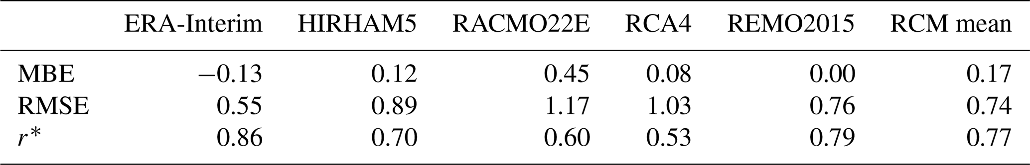
^* All are statistically significant at p<0.01.

Averaged in space, the RCM evaluation runs reproduce generally, but not perfectly, the temporal evolution of the E-OBS HWMId as shown in Fig. 2a. Years with high HWMId values (1994, 2003, 2006, and 2007) are captured by all the RCMs. However, the RCMs fail in reproducing the ranking of these years by occasionally overestimating or underestimating the HWMId values. For example, RACMO22E overestimates HWMId excessively in 1995 as does RCA4 in 1997. Reflecting on the distribution function as shown in Fig. 2b, the HWMId values simulated by the RCMs show an overestimation of the 75th percentile and the median, while deviations for the 25th percentile are smaller with REMO2015 showing an underestimation and HIRHAM5 and RACMO22E overestimations. Both HIRHAM5 and the multi-RCM mean show a better representation of the observed IQR but shifted to higher values and, in addition, with a shorter right tail, which means too weak heat wave extremes. At the same time, and in contrast to E-OBS and ERA-Interim, all the RCMs have individual years with HWMId values lower than the observations, indicating that there are also underestimations of heat waves. Among the selected RCMs, HIRHAM5 outperforms the others in reproducing the temporal evolution of the regional mean (Table 3). Like the case of spatial measures, the multi-RCM mean has also a generally smaller RMSE and a higher r of temporal measures than most of the individual RCMs.

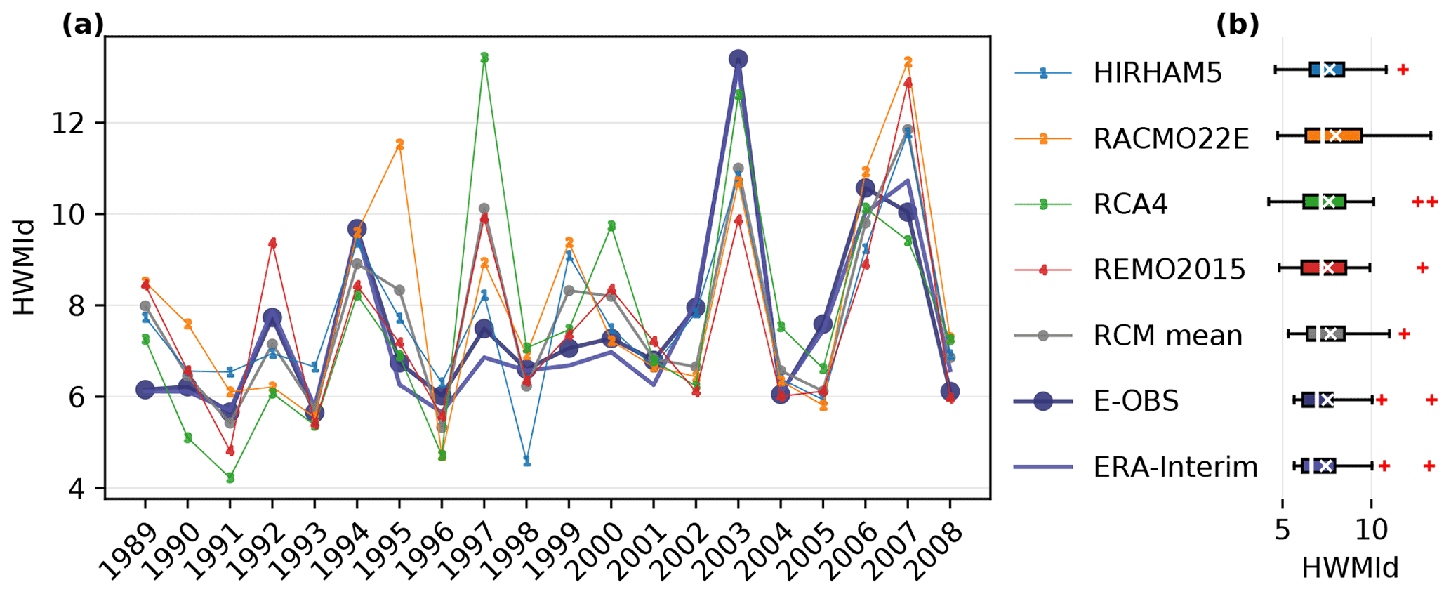
Figure 2 Regional mean HWMId from 1989 to 2008 in the four RCM evaluation runs, the multi-RCM mean, E-OBS, and ERA-Interim: (a) temporal evolution, and (b) corresponding box-plot. In each box-plot, the box limits represent lower and upper quartiles, the white line and “x” marker inside the box are the median and the mean, respectively and the outliers marked with red plus signs outside of the whiskers lie at least 1.5 times the IQR away from the box limits.

Table 3 Similar to Table 2 but with temporal measures for the time series of regional mean HWMId from 1989–2008 (corresponding to Fig. 2).

^* All are statistically significant at p<0.01.

3.2 Evaluation of heat waves in GCM-driven RCMs under the recent past climate

A similar comparison, as for the ERA-Interim-driven runs discussed above, was conducted for the GCM-driven runs but focused only on the spatial patterns. The influence of the shift of driving data from ERA-Interim to GCM simulations can be seen by comparing Table 4 with Table 2, where the reference period as the basis of HWMId is identically 1989–2008. The GCMs perform poorly in simulating spatial characteristics of HWMId compared to ERA-Interim (RMSE: 1.02–1.26 vs. 0.55, and r: 0.17–0.43 vs. 0.86), whereas GCM-driven RCM simulations show similar results as the ERA-Interim-driven ones, which is particularly obvious for RMSE (0.97–1.37 vs. 0.76–1.17). This implies an improvement in the representation of the spatial characteristics of HWMId introduced by the dynamical downscaling with RCMs. Moreover, the improvement seems to depend strongly on the model (e.g., RCA4 has a relatively weak spatial r).

Table 4 Spatial MBE, RMSE, and r for the climatological mean HWMId over 1989–2008 (with reference period also as 1989–2008) in the selected GCM simulations and the GCM-driven simulations that compose the RCM simulation matrix (columns for RCMs and rows for their driving GCMs), with E-OBS as reference. For each statistic, an additional row is given for the column mean (i.e., along the GCM dimension) of the driving GCM simulations and the RCM simulation matrix.

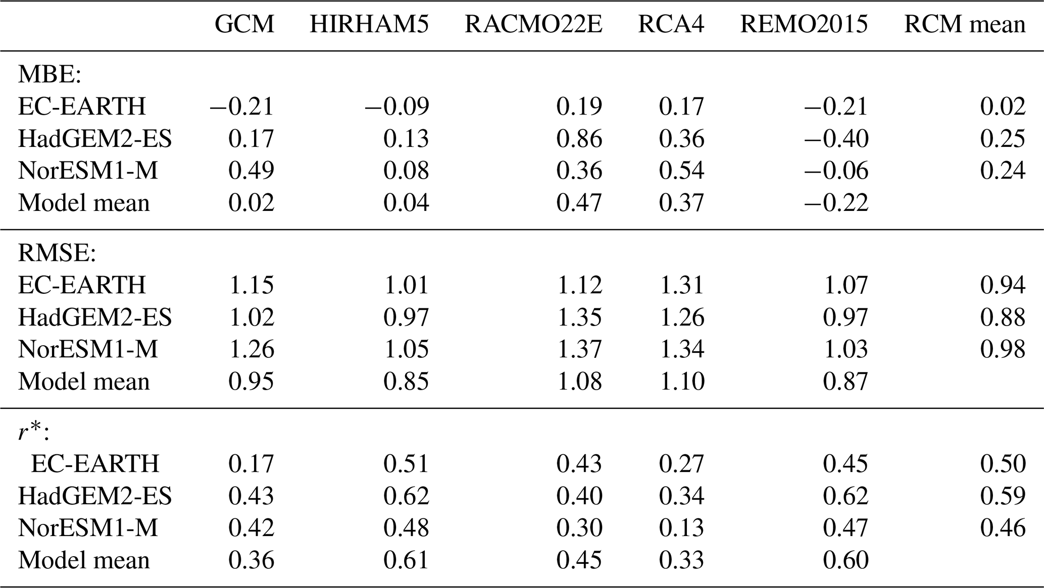
^* All are statistically significant at p<0.01.

Figure 3 presents the spatial pattern of climatological mean HWMId under the recent past climate. With reference to Fig. 1, a shift in time for both the reference period as the basis of HWMId and the period of investigation should be noted. As expected, due to the relatively large overlap in time, the observed spatial distribution under the recent past climate, as revealed by E-OBS (Fig. 3), is similar to that in the evaluation period (Fig. 1) but the shift in time has led to an increase from an average of about 7.5 to about 8.0 on a continental basis with an increase mainly in the Mediterranean parts of Europe. The GCMs capture some of the observed spatial pattern but miss out both in detailed structure and amplitude (Fig. 3). The observed west-east gradient is hardly seen in the GCM simulations: EC-EARTH and HadGEM2-ES report no difference between the western and eastern parts (divided by the white line on the map), while NorESM1-M shows a west-east gradient of 1.3, which is even higher than for E-OBS but simulates excessively high HWMId values in the easternmost part of the domain. The downscaling with RCMs improves the representation of the observed spatial pattern by reproducing the west-east gradient, as well as revealing small-scale processes, such as orographic effects which are not well represented by the GCMs due to their coarse resolution. In general, the RCMs (other than a few cases of RACMO22E and RCA4) show smaller RMSE and higher r compared to their driving GCMs (Table 5). Similar to the evaluation runs (Table 2), the multi-RCM (row) means driven by a GCM simulation show better performance compared to most of the individual RCMs. This is also true for the GCM dimension, i.e., for each RCM, the ensemble mean across the three driving GCMs outperforms the individual ensemble members.

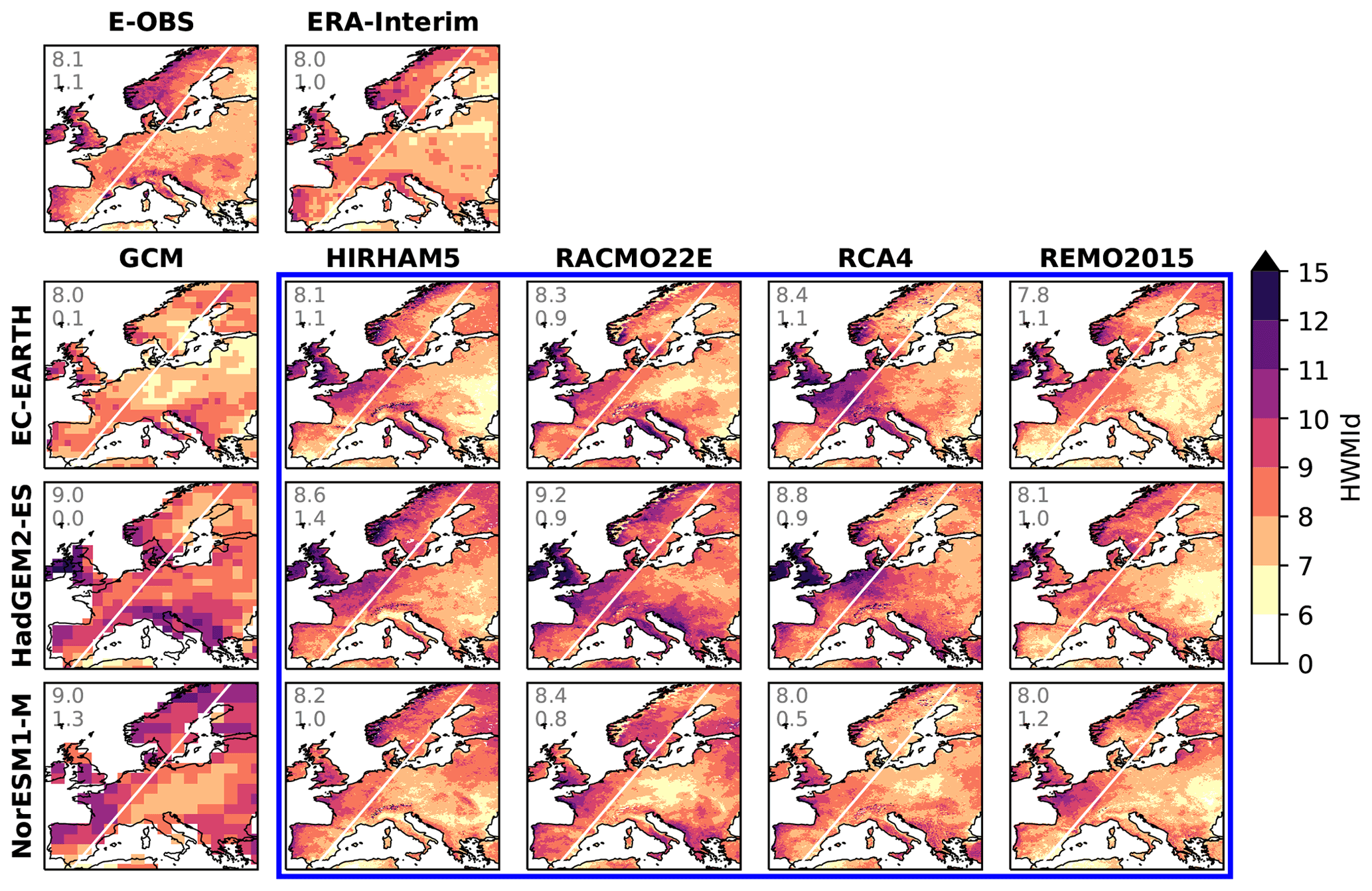
Figure 3 Climatological mean HWMId under the recent past climate (1981–2020) in the RCM simulation matrix (inside the blue rectangle; columns for RCMs and rows for their driving GCMs) as well as the driving GCM simulations. Data from E-OBS and ERA-Interim are also shown for comparison. The two numerals in each map show the area-weighted average over the entire domain and the difference between western and eastern parts divided by the white line.

Table 5 Similar to Table 4 but for the recent past climate (1981–2020, with the reference period of HWMId as 1981–2010).

^* All are statistically significant at p<0.01.

Furthermore, we also looked into the differences along the GCMs in representing HWMId and how the RCMs respond to them when driven by these GCMs. We want to point out that there is no accordance on which GCM performs best among the three in reproducing the spatial pattern of HWMId in E-OBS when considering different performance indicators, e.g., EC-EARTH has the smallest MBE/RMSE, whereas HadGEM2-ES has slightly higher r (Table 5). Meanwhile, the “best” GCM according to a performance indicator may not necessarily secure the best downscaling among the different driving GCMs for an RCM. We also observed a large spread in the regional average across the GCMs, which is reduced by all RCMs. Moreover, for each RCM driven by the three GCMs, the downscaling behaves consistently despite the large difference in the spatial pattern of HWMId between the driving GCMs. This can be reflected by the fact that for each RCM we observed lower RMSE and higher r (of spatial measures) between the RCM simulations than between the driving GCMs (Table S1). Likewise, when driven by one GCM, the simulations of different RCMs also most often tend to be more similar to each other than to the driving GCM (i.e., higher RMSE and lower r within the “GCM” column compared to other columns in Table S2). Thus, it is interesting to explore the influences of driving data versus model physics on the uncertainty for the RCMs in simulating heat wave magnitudes under the recent past climate.

Along the RCM dimension of the matrix (i.e., RCMs with the same driving GCM), the ensemble spread of HWMId values is on average close to one fifth of the ensemble mean on a continental basis (Fig. 4). A slightly lower spread/mean ratio is observed along the GCM dimension (Fig. 5), indicating that the uncertainties associated with driving data are of similar magnitude as those associated with model physics. However, different features can be observed in the spatial pattern of the ensemble spread along the two dimensions. As presented in Fig. 4, the ensemble spread along the RCM dimension shows high values mostly in mountainous areas such as the Scandinavian mountains and the Alps, suggesting the disagreement in the orographic effects on heat wave magnitudes across the RCMs as one of the major sources of uncertainty that is associated with model physics. Aggregating on the GCM dimension (i.e., calculating mean and spread for each RCM with different GCMs), the ensemble means (first row of Fig. 5) reveal a similar spatial pattern, whereas the spreads (second row of Fig. 5) show considerable differences in the spatial pattern. A quantitative analysis regarding the similarity based on RMSE and r is presented in Table S3. Higher r values between RCMs than between any RCM and the driving GCMs, in combination with lower RMSE scores (in all but one), indicate that the RCMs tend to converge in the ensemble mean and spread along the GCM dimension. Compared to the ensemble mean, however, the r values are much lower for the ensemble spread. This observation implies that the uncertainties of GCMs in simulating heat wave magnitudes are not simply inherited by RCMs but are transformed in a nonlinear manner due to the complex model dynamics and physics.

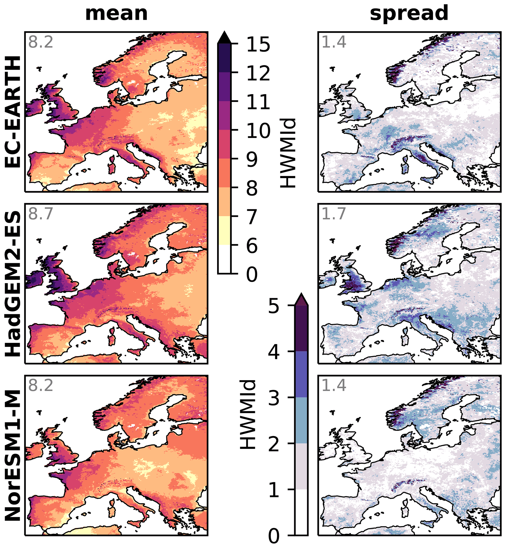
Figure 4 Ensemble mean and spread (maximum − minimum) of simulated HWMId under the recent past climate (1981–2020) for each row in the RCM simulation matrix indicating the uncertainty associated with different RCMs. The numeral in each map shows the area-weighted average.

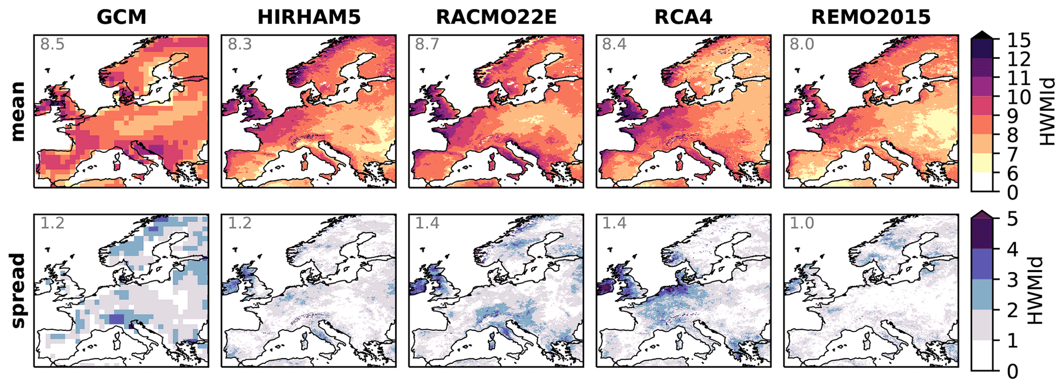
Figure 5 As Fig. 4 but for the columns of the RCM simulation matrix indicating the uncertainty associated with driving data (boundary and initial conditions). Ensemble mean and spread of the driving GCM simulations are also presented for comparison.

3.3 Simulated future change in heat wave magnitudes

The change in the climatological mean HWMId under RCP8.5 relative to the recent past climate was investigated for two future periods within the century: the nearest decades (2021–2060) and the end of the century (2061–2100). Figure 6 presents the spatial pattern in each of the simulations. The HWMId increases strongly at the end of the century, with approximately more than a factor of three compared the nearest decades. The HWMId patterns generally stay similar within the two observed time periods, according to the spatial r (Fig. 6b) for the two periods. Similar to the results of the recent past climate (Sect. 3.2), a large spread in ΔHWMId is seen across the GCMs (5.8–12.8 and 21.6–48.4 for the nearest decades and the end of the century, respectively; Fig. 6). The RCMs decrease the spread (4.9–8.7 and 15.0–31.9 for the nearest decades and the end of the century, respectively; Fig. 6), reflecting less change than two out of the three driving models (i.e., HadGEM2-ES, NorESM1-M). The spatial pattern of ΔHWMId among the RCM simulations is similar both along the RCM dimension and the GCM dimension, indicating a stronger rise in northern and southern Europe but comparatively moderate for the central domain. This partly differs from the GCM simulations, which tend to show a more pronounced south-north gradient in the increase in HWMId. It also differs from the climatological mean HWMId under the recent past climate, which displays a generally west-east gradient (Fig. 1). The ensemble spread, along either the RCM dimension (Fig. 7) or the GCM dimension (Fig. 8), has a magnitude most often exceeding half of the ensemble mean on a continental basis and to some extent follows the spatial distribution of the ensemble mean (with spatial r from 0.50 to 0.92; not shown). This suggests that the driving GCMs and the RCMs contribute about equally to the uncertainty in simulating climate change in heat wave magnitudes. For the ensemble spread, however, high values in mountainous areas are more common along the RCM dimension than along the GCM dimension. This underlines again that processes related to orography are a major source of uncertainty related to future changes in heat wave magnitudes in Europe.

Figure 6 Change in climatological mean HWMId in the nearest decades (a: 2021–2060) and in the end of the century (b: 2061–2100) relative to the recent past climate (Fig. 3), with results from the RCM simulation matrix placed inside the blue rectangles. The first numeral in each map shows the area-weighted average, and the second (only presented in b) is the spatial r between the two periods (with “^*” indicating statistical significance at p<0.05).

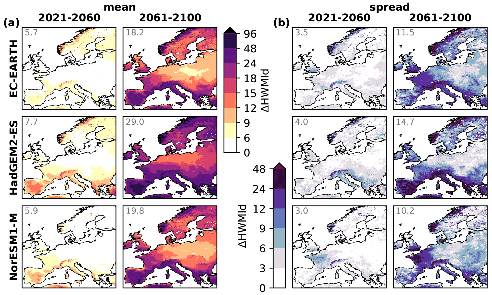
Figure 7 As Fig. 4 but for the climate change in HWMId.

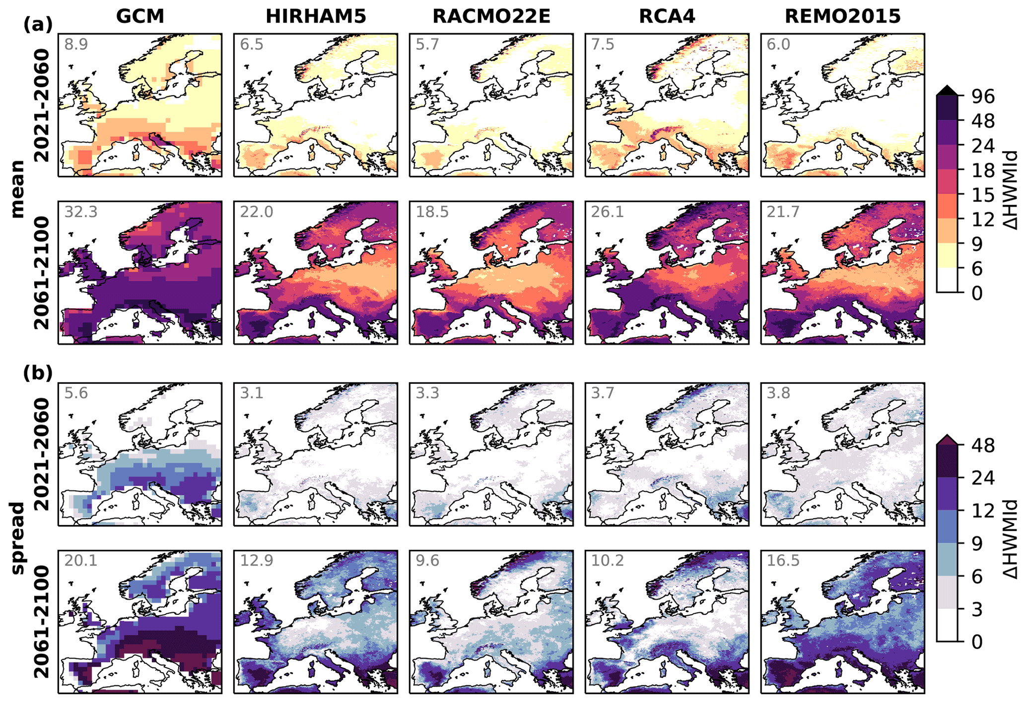
Figure 8 As Fig. 5 but for the climate change in HWMId.

The percentages of the land area exceeding certain HWMId levels (Fig. 9) provide a special form of survival function (complementary cumulative distribution function) to investigate the probability distribution of climatological mean HWMId values across the domain regardless of geophysical location. All model simulations can reproduce the E-OBS data probability distribution of HWMId values (solid lines) within ±15 %. A considerable rise in the future is projected by all the simulations. In the end of the century (2061–2100), the entire domain is projected to reach HWMId values higher than those experienced until now under the high emissions scenario RCP8.5. The rise occurs across the whole probability range at an approximately exponential rate, i.e., increases between every two neighboring periods are approximately the same as mapped to the logarithmic scale applied to Fig. 9. The rise is even stronger for the tail of HWMId distribution. As indicated in Fig. 6 the RCMs show a tendency to smooth the change signal in the driving GCM simulations, particularly when driven by HadGEM2-ES and NorESM1-M. The only exception is the RCA4 downscaling EC-EARTH. Again, we note that the RCMs generally are more alike than their driving GCMs, although RCA4 shows a pattern closest to the GCMs. Finally, we observe that the spread between the RCMs, and hence the uncertainty, greatly increase over time.

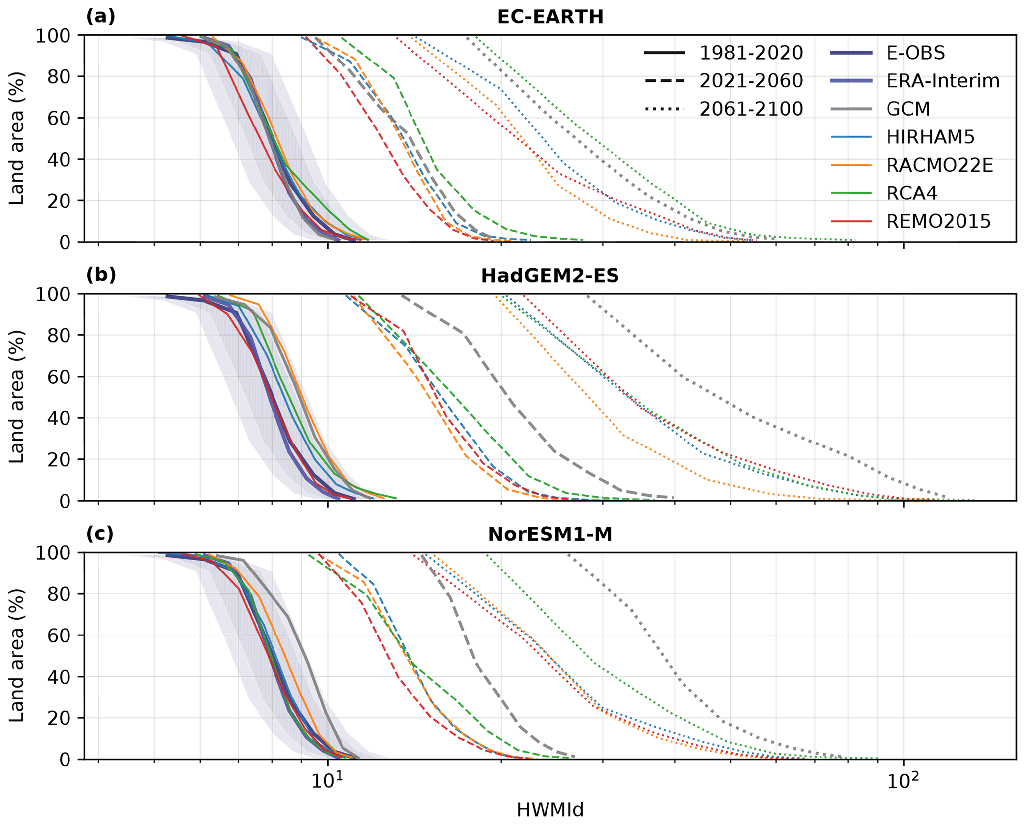
Figure 9 Percentage of the land area exceeding certain HWMId levels during the defined three periods (identified by the line styles), grouped by the driving GCMs: (a) EC-EARTH, (b) HadGEM2-ES, and (c) NorESM1-M. Colors represent different RCMs and gray the GCMs themselves. Data from E-OBS and ERA-Interim are also shown for comparison under the recent past climate. The shaded areas indicate within ±10 % (relatively dark) and ±15 % (light) of E-OBS data. Note that a logarithmic-scale x-axis is used.

Probability distributions are also investigated for the region-wide annual HWMId values in the defined three periods, as shown in Fig. 10. As revealed by E-OBS and ERA-Interim, the region-wide HWMId for the recent past climate is represented by a positively skewed distribution, or rather a quasi-log-normal distribution (as demonstrated by the quasi-normal shape of the distribution in Fig. 10b with a logarithmic scale x-axis). As discussed for the ERA-Interim driven simulations (Fig. 2), the GCM-driven RCMs can also to some extent capture the shape of the distribution as well as the median, but with a wider value range for each simulation. Most of the simulations keep the shape of distribution as the values increase in the future (especially for the nearest decades), whereas some (e.g., HadGEM2-ES, RCA4 driven by EC-EARTH, and RACMO22E driven by NorESM1-M) display a distribution even with a negative skewness for the end of the century (mostly visible with the logarithmic axis presented in Fig. 10b), which indicates that high HWMId values would become more common under the high emissions scenario RCP8.5. In addition to increasing levels of HWMId, the spread defined by the ranges also increases in the future. With a logarithmic scale x-axis, we observe interesting features in the change signal: (i) the mean and the median increase approximately at an exponential rate and (ii) the width of the logarithmically transformed distribution does not change much from one period to another, i.e., a rise approximately at an exponential rate for both the low and high ends of HMWId values.

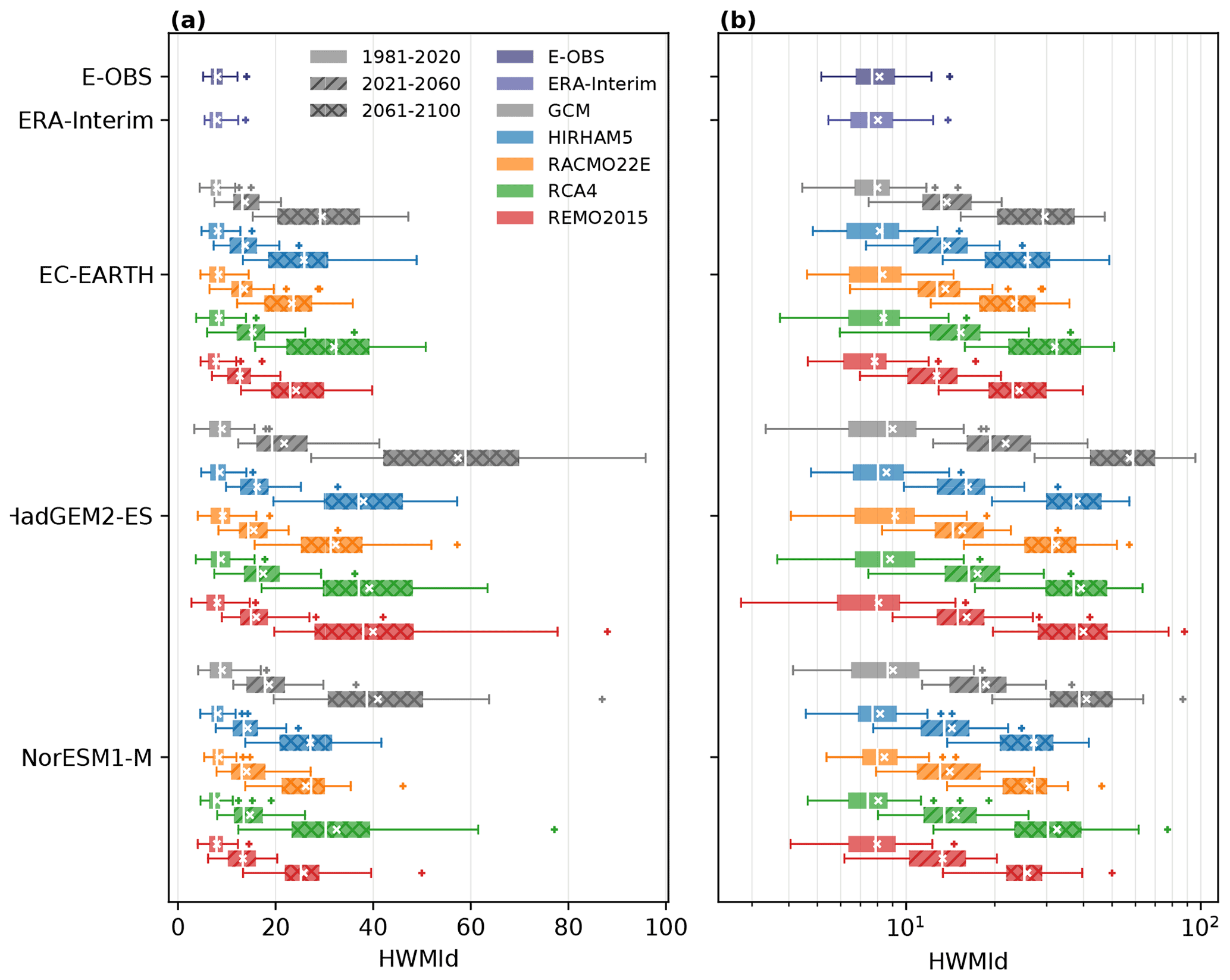
Figure 10 Box-plot for regional mean HWMId values under the defined three periods (indicated by filling patterns) in the simulation matrix of RCMs as well as the driving GCM simulations. Data are presented on different scales: (a) linear, and (b) logarithmic. Within each group (with one GCM), RCMs are identified by colors. Data from E-OBS and ERA-Interim are also shown for comparison under the recent past climate.

4 Discussion

4.1 Added value of RCMs compared to GCMs

With more small-scale processes being resolved, added value is expected from dynamical downscaling with an RCM compared to its driving GCM on the regional scale. Indeed, a large number of previous studies (e.g., Torma et al., 2015; Rummukainen, 2016; Strandberg and Lind, 2021) have reported such added value by RCMs in many respects. Thus, it is of great interest if RCMs create added value also for heat wave magnitudes. To realistically represent HWMId, a model must be able to capture not only the mean magnitude but also the intra-annual temporal evolution of daily T_max. Before discussing any potential added value we assess to what degree the studied RCMs can represent the observed HWMId under the historical climate when driven by reanalysis data (i.e., perfect boundary conditions). We showed in Sect. 3.1 that the ERA-Interim-driven RCM runs generally reproduce the spatial and temporal patterns of the observed annual heat wave magnitudes over Europe. However, the RCMs clearly add their own signatures to the results leading to a larger variability in the spatial distribution of HWMId than reflected in E-OBS and ERA-Interim (Fig. 1). Even larger variability was found in the HWMId spatial distribution of the years 1994, 2003, 2006, and 2007 (Figs. S4–S7) than for the climatological mean, although these events, which were reported by the news headlines (Russo et al., 2015), are generally captured (Fig. 2a) by the RCMs when driven by ERA-Interim. Another interesting observation is that RCA4, which performs worse than the other RCMs (Table 2) in representing climatological mean, best reproduces the HWMId spatial distribution of the year 2003 (Fig. S5 and Table S4). A more in-depth event-based analysis would be needed to see which events are large-scale triggered from the boundaries of the RCMs and thereby picked up by the RCMs, and which events are triggered inside the RCM domain and therefore possibly missed or reproduced differently by the different RCMs. One example of a large-scale-driven event could be the year 2003, where the HWMId is picked up clearly by all the RCMs in its high intensity (Fig. 2a).

The three GCM simulations accounted for roughly reproduce the observed patterns for the recent past climate, but miss out on details in structure and amplitude (Fig. 3). The RCMs downscaling these GCMs do well in adding more detailed geographical patterns and, furthermore, pull the results closer to the observations. Again, the RCMs add their own pattern, e.g., the lower HWMId values over eastern Europe in REMO2015. Signatures of the RCMs can also be demonstrated by the high similarity in HWMId spatial pattern between the simulations for each RCM despite a large difference between the driving GCMs (Table S1). Certainly, the RCMs also inherit signals from their driving GCMs. This is clearest for RACMO22E among the four RCMs, as the simulations with RCAMO22E show the highest r (except when driven by NorESM1-M) and the lowest RMSE against its driving GCMs (Table S2). Despite the inherited signals from the driving GCMs, the simulations of different RCMs when driven by the same GCM generally share higher similarities than with the driving GCM (Table S2), implicating a coherence for RCMs in representing heat wave magnitudes when downscaling GCMs.

Some studies (e.g., Schiermeier, 2010; Kerr, 2011) show that uncertainty may increase when downscaling GCMs with RCMs as biases from the GCMs are conveyed to the RCMs and RCMs additionally add their own biases, referred to as the “cascade of uncertainty” (e.g., Wilby and Dessai, 2010). However, many other studies (e.g., Torma et al., 2015; Di Luca et al., 2016; Rummukainen, 2016; Sørland et al., 2018; Strandberg and Lind, 2021) indicate that RCMs can also add value to the driving GCM simulations. This study demonstrates the added value for heat wave magnitudes that have so far not been studied as extensively as for other aspects of climate and climate change, reflected in adding more detailed geographical patterns and pulling the results closer to the observations (Fig. 3; Tables 4 and 5). Such added value confirms the usefulness of RCMs for downscaling coarse-scale GCM simulations, because downscaling can be considered as an act of adding useful details to those already provided by GCMs: details about how local geography influences the local climate (as in this case) and details about how local climates depend on the ambient large-scale conditions and teleconnections that the GCMs skillfully reproduce. Moreover, RCMs may also more realistically represent some atmospheric processes relative to the GCMs (e.g., Prein et al., 2016). Our analysis of the ensemble spread along the GCM dimension, reflecting uncertainty associated with driving data, reveals that the RCMs alter the spatial HWMId pattern from their driving GCM simulations, and that the alteration is different between the RCMs (Fig. 5 and Table S3). This, on the other hand, suggests that the uncertainties of GCMs in simulating heat wave magnitudes would be transformed by RCMs in a complex manner, rather than simply inherited, due to the nonlinear nature of model dynamics and physics, thus questioning the concept of “cascade of uncertainty”.

To reveal the specific factors and processes behind the added value of RCMs in simulating heat wave magnitudes, however, further analysis is required. Table 4 and Fig. 3 clearly show that RCMs capture the HWMId better than the GCMs for the recent past climate. Some spatial features of HWMId showing orographic traces, thereby considered to be related to orographic effects, can be seen as one aspect of the added value of RCMs as GCMs cannot represent such features due to a too coarse spatial resolution. An interesting finding of this study is that the orographic effects are, however, represented differently across the RCMs (i.e., the large ensemble spread along the RCM dimension; Fig. 4), suggesting that the representation of orographic effects, possibly related to dynamical and/or thermodynamical interaction with parameterizations, is meanwhile one of the major sources of uncertainty. This supports the statement by Sørland et al. (2018) that increasing the spatial resolution should not be the single factor contributing to the added value of RCMs.

4.2 Possible processes behind the simulated climate change signals

The RCMs, as well as the driving GCMs, project a rise in HWMId values at an exponential rate under RCP8.5 on the European continent, as we can observe the linear shape of time series when plotting on a logarithmic scale (Fig. S8). As a result, heat waves more severe than the most severe one that has been recorded until now are projected to occur almost every year at the end of the century if we follow the high-end emission pathway (RCP8.5). According to the definition of HMWId, the approximately exponential rise can be expected because the projected warming will on the one hand increase the daily magnitude (Eq. 2) and on the other hand simultaneously extend the duration. Apart from the agreement on the future severity of heat wave magnitudes under RCP8.5, the RCMs modify the future climate change signals projected by the driving GCMs, tending to moderate the rise in HWMId values and also deliver some different features in the spatial pattern. The underlying drivers of heat waves may be related to land-atmosphere interactions as well as atmospheric processes (Horton et al., 2016; Liu et al., 2020). For example, plant physiological CO₂ response may have a positive effect on T_max (Schwingshackl et al., 2019) and thereby on HWMId values. Understanding how RCMs differ from GCMs in representing processes that modify the climate change signals can have implications for how to utilize model projections in studies on climate change mitigation and adaptation.

Here, rather than directly looking into the associated processes, we investigate the corresponding climate change signals in annual mean T_max (Fig. S9), dry days (Fig. S10), and P−E (Fig. S11). As the HWMId is directly calculated from daily T_max, the increase in annual T_max provides a warming background that the surge in HWMId is associated with. An increase in the annual number of dry days may indicate a higher tendency for longer warm spells and hence a rise in HWMId. Compared to the number of dry days, P−E (or effective precipitation if we do not consider the variation in runoff) is more strongly related to dry soil conditions; the correlation between effective precipitation and HWMId may reveal the effect of land-atmosphere feedbacks, as the deficit in soil moisture may reduce latent heat flux allowing temperatures to rise further (Zhang et al., 2020).

The RCMs dampen the increase, and to some extent modify the spatial pattern, in the annual mean of daily T_max in HadGEM2-ES and NorESM1-M (Fig. S9 and Table S5). This could potentially explain the more moderate rise in HWMId simulated by the RCMs compared to the driving GCMs. EC-EARTH and its downscaling by the RCMs show a similar level of increase as well as a similar spatial pattern in the annual mean of daily T_max (Fig. S9 and Table S5), and we recognize that they also project a similar rise in HWMId (Fig. 6). According to Schwingshackl et al. (2019), these results may be linked to the positive effect of plant physiological CO₂ response on T_max, since the GCMs except for EC-EARTH consider this response but all the RCMs do not. That RCMs are better at representing near-surface processes that are important for reducing the drying feedback is also considered a reason (Sørland et al., 2018). For the annual number of dry days (Fig. S10), on a regional average the RCMs also reduce the increase from their driving GCMs, but with a few exceptions (e.g., HIRHAM5 downloading EC-EARTH and HadGEM2-ES). For annual P−E (Fig. S11), on a continental basis the RCMs, except for HIRHAM5, show a smaller decrease (or larger increase) than the driving GCMs. In general, these results are consistent with Coppola et al. (2021) who discussed similar indices.

We further examined the spatial correlation between the change in HWMId and that in each of the three indices accounted for, to find any trace of whether, and if so how, the drying processes (of either atmospheric or soil) regulate the spatial pattern of ΔHWMId. For the detailed spatial pattern of ΔHWMId, it cannot be explained by the change in the annual mean of daily T_max alone, even though HWMId is calculated based only on daily T_max. This is especially true for GCM simulations as they have a poor spatial correlation between ΔHWMId and ΔT_max (Fig. S9). All the GCM and RCM simulations agree on the high ΔHWMId in southern Europe (Fig. 3), which may be amplified by the local drying trend projected (Figs. S10 and S11), while in northern Europe where rapid warming is projected (Fig. S9), high ΔHWMId is seen in the RCM simulations only (Fig. 3). The r values in Figs. S9–S11 show that the general warming, compared to drying, plays a small role in regulating the spatial pattern of ΔHWMId in GCM simulations, different from the case of the RCMs. This echoes the varying importance of drying in influencing ΔHWMId in northern Europe for GCM and RCM simulations, i.e., the wetting trend in northern Europe, projected by both the GCM and RCM simulations (Figs. S10 and S11), seems to dampen the local ΔHWMId within the GCM simulations, but has little impact on the local ΔHWMId within the RCM simulations. It is interesting and deserves further study which factors cause the varying importance of drying in influencing heat wave magnitudes and how differently GCMs and RCMs represent these factors.

As a preliminary effort concerning only the spatial pattern, the above analysis is, however, far from building clear causal links. Moreover, we are not yet clear about what is leading to the weaker drying trend in the RCM simulations. Atmospheric blocking, with adiabatic warming of sinking air and anomalous clear sky radiative forcing, is an important driver of heat waves (e.g., Bieli et al., 2015; Schaller et al., 2018). According to Masato et al. (2013), the three CMIP5 GCMs assessed show a decrease in summertime North Atlantic blockings and an increase in blockings over eastern Europe or Russia indicating an eastward shift of the blocking activity. This implies that the underlying processes of ΔHWMId are possibly beyond the atmospheric dynamics. It is of interest whether, and if so how, the RCMs modify the climate change signals of atmospheric blocking from their driving GCMs, and whether this modification is related to the differences in ΔHWMId patterns between GCMs and RCMs as presented here, which is worth further study, although representing atmospheric blocking is considered a challenge (e.g., Masato et al., 2013; Davini and D'Andrea, 2016; Jury et al., 2019). Regarding the representation of the effect of land-atmosphere interactions, investigations detailed into different sets of parameterizations in GCMs and RCMs as well as some additional sensitivity experiments may be necessary for a better understanding.

4.3 Other matters

A full simulation matrix without gaps facilitates a fair comparison after aggregating along either the GCM or the RCM dimension. This prerequisite limits the size of the RCM simulation matrix available for analysis. The limited size of the GCM-RCM simulation matrix could be a shortcoming influencing the robustness of the results in the study, especially for the uncertainty analysis where the uncertainty is described by the spread (maximum −  minimum) across three or four ensemble members. In fact, we conducted the same analyses on another GCM-RCM simulation matrix (GCMs: EC-EARTH, HadGEM2-ES, and MPI-ESM-LR; RCMs: CCLM4-8-17, HIRHAM, RACMO22E, and RCA4) and derived similar results (not shown), which can alternatively support the conclusions herein.

The HWMId can also be applied to other temperature variables, but with different processes/impacts involved. For example, the HWMId applied to daily minimum temperatures serves as a measurement of heat wave magnitude also taking the nighttime cooling effect into account (Russo et al., 2015). As another example, the Apparent Heat Wave Index (AHWI, Russo et al., 2017) is the HWMId applied to daily apparent temperature, which also considers the impact of air humidity on human beings. Such variants of HWMId are being considered for future studies.

5 Summary and conclusions

By deploying the HWMId index, the study addresses how four different RCMs downscaling (i) reanalysis and (ii) three different GCMs, represent European heat wave magnitudes.

Initially, the performance of the RCMs in reproducing historical heat wave magnitudes is evaluated by comparing the ERA-Interim-driven evaluation runs of the RCMs with E-OBS. It shows that the RCMs generally capture most spatial and temporal features of the observed HWMId when considering climatological mean and regional mean, respectively. Our results also prove the added value of RCMs over GCMs in representing the observed heat wave magnitudes. Compared to the driving GCMs, the RCMs generally have lower RMSE and higher r against the observational data for the climatological mean of HWMId values under the recent past climate. The RCMs generally improve the spatial pattern of HWMId across the European continent compared to the driving GCMs. In addition, the RCMs reveal some small-scale features (e.g., relating to orographic effects) that the GCMs fail likely due to their coarse resolutions. The closest agreement with observations is seen for the RCM ensemble mean.

A rise in HWMId at an exponential rate is projected consistently by all the GCM and RCM simulations accounted for in the study, probably because the warming boosts both the intensity and duration of heat waves. However, the RCMs modify some features of the climate change signals in the driving GCM simulations. A somewhat more moderate rise across the European continent is projected by the RCMs, as a corresponding result of the reduced warming. The RCMs also differ from the driving GCMs in the spatial pattern of the climate change signals of HWMId.

We also analyzed the uncertainties of the GCM-RCM simulation matrix in simulating heat wave magnitudes. The results show that the uncertainty associated with choice of RCM is of similar importance as with driving data. The ensemble spread/mean ratio is approximately one fifth for the present climate HWMId and over half for the climate change signals. A major source of the uncertainty associated with the RCMs appears to be associated with the representation of orographic effects. The RCMs reduce the large ensemble spread across the GCM simulations though, especially for the climate change signals in HWMId. Moreover, no consistent spatial pattern is observed in the ensemble spreads along the GCM dimension for different RCMs. Consequently, the results indicate that the uncertainties of GCMs in simulating heat wave magnitudes would not be simply inherited by RCMs but are transformed in a complex manner due to the nonlinear nature of model dynamics and physics.