Modelling forest ruin due to climate hazards

Estimating the risk of forest collapse due to extreme climate events is one of the challenges of adapting to climate change. We adapt a concept from ruin theory, which is widely used in econometrics and the insurance industry, to design a growth–ruin model for trees which accounts for climate hazards that can jeopardize tree growth. This model is an elaboration of a classical Cramer–Lundberg ruin model that is used in the insurance industry. The model accounts for the interactions between physiological parameters of trees and the occurrence of climate hazards. The physiological parameters describe interannual growth rates and how trees react to hazards. The hazard parameters describe the probability distributions of the occurrence and intensity of climate events. We focus on a drought–heatwave hazard. The goal of the paper is to determine the dependence of the forest ruin and average growth probability distributions on physiological and hazard parameters. Using extensive Monte Carlo experiments, we show the existence of a threshold in the frequency of hazards beyond which forest ruin becomes certain to occur within a centennial horizon. We also detect a small effect of the strategies used to cope with hazards. This paper is a proof of concept for the quantification of forest collapse under climate change.

1 Introduction

Extreme events such as droughts and heatwaves are climate hazards that have short- and long-term effects on forests. The accumulation of drought and heat stress in forests due to recent events might lower their resilience to future extreme events (e.g. Wigneron et al., 2020; Flach et al., 2018; Bastos et al., 2020; Anderegg et al., 2015a). It has been observed that such events increase the chance of tree mortality (Anderegg et al., 2013). This increase in tree mortality probability challenges the survival of tree species in some regions of the world (Zeppel et al., 2011; Lindenmayer et al., 2016). The mechanisms leading to tree mortality include complex physiological processes that can depend on the tree species and type of hazards involved (e.g. Choat et al., 2012).

Most studies on tree death are based on direct or indirect observations of the behaviour and growth parameters of trees. They give precious information on the observed global response of forests to climate hazards, but they are also inherently limited to the observation period used and have mostly focused on a few key observed events (e.g. Rao et al., 2019). This can hinder the development of the statistical description needed to build projections or estimate risk (Field et al., 2012) as a response to climate change. Here, risk is considered to be the probability distribution of a failure (e.g. irreversible damage or death) due to climate hazards (Katz, 2016).

The potential disappearance of a whole forest or a given tree species due to changes in climate features can be considered a tipping point for climate change. There is ample literature on tipping points in the climate system, i.e. climate thresholds beyond which ecosystems change their behaviour (Lenton et al., 2008; Levermann et al., 2012). These papers have defined methodologies for identifying climate thresholds beyond which ecosystems are endangered. They have been used to infer tipping points of forests (Reyer et al., 2015; Pereira and Viola, 2018).

The key concept of this paper is the use of so-called ruin theory to provide estimates of the probability of such tipping points. Many papers in the econometrics literature that describe ruin models for insurance and finance have been published since the seminal work of Lundberg (1903). A mathematical and statistical framework (Asmussen and Albrecher, 2010) has been used to help determine the optimal parameters of such models, so that insurers or investors limit the risk of losing their investment and maximize their gain. Ruin models are used to describe the probability that a company which grows with regular income will become bankrupt due to external hazards. To the best of our knowledge, such models have never been adapted for use in the environmental sciences.

We chose to investigate trees or forests because trees are adapted to live for a long time and can survive adverse climatic conditions during a given year, in contrast to annual plants. Process-based growth models for trees can be devised (e.g. Han and Singh, 2020), and observations of tree mortality are available (e.g. Choat et al., 2012). Tree growth is affected by climate variations in various ways. Heatwaves and droughts can alter (and lower) tree reserves and the capacity of trees to grow during the years following an extreme climate event, which affects their average growth and can increase the probability of tree mortality (von Buttlar et al., 2018; Sippel et al., 2018). For this reason, trees contain a large amount of nonstructural carbohydrates (NSCs). These NSC reserves allow trees to rapidly build large surfaces of leaves (potential productivity is related to foliage area) at the time of leaf onset during the subsequent year. NSCs also help with leaf renewal following defoliation (caused by frost or insects, for instance) and, more generally, provide the necessary energy for metabolism (e.g. to protect the tree from pathogenic diseases). Hence, part of the annual productivity of a tree is devoted to its accumulation of carbohydrate reserves (i.e. these reserves are larger than required to initiate the leaf phenological cycle during the following year). As there is a competition between NSC reserves and plant growth for the allocation of assimilates, the plant does not accumulate reserves indefinitely; the reserves tend to reach an optimum level (Barbaroux et al., 2003). Climate hazards can reduce the quantity of assimilates allocated to the reserve (He et al., 2020). This can be caused directly by a reduction in productivity, but climate hazards can also indirectly cause plant damage, such as xylem embolism, which can kill trees in extreme cases (especially in young trees). This process kills only parts of mature trees, which affects the total amount of NSCs and the development of new foliage and jeopardizes the ability of the tree to grow in the following years. So, even though this effect does not directly impact NSC reserves, it has equivalent consequences for tree growth in the years following climate hazards. Several studies have investigated the physiological processes leading to tree mortality based on empirical observations (Adams et al., 2009; Bigler et al., 2007; Bréda and Badeau, 2008; Villalba and Veblen, 1998; Matusick et al., 2018). Those studies compared relative tree ring growth between dead and healthy surrounding trees of the same diameter during the years prior to tree death. Since it removes annual climate effects, such a comparison is a good proxy for the difference in NSC reserves. Those studies concluded that dying trees have a systematically lower level of reserves than living trees. Hence, even if trees are not fully depleted of NSCs, there is a critical level of NSCs below which trees cannot recover, so they die. These studies suggest that the levels of NSCs in trees are good indicators of possible forest dieback. Allocation to NSC reserves can hence be compared to an insurance system where, each year, part of the productivity is “paid” to the insurance (i.e. NSCs for trees) which, in return, can be mobilized in the case of damage. Therefore, “ruin” occurs when the amount of NSCs drops to a critical level below which the probability of tree death in the short term becomes very likely. This loosely justifies drawing a parallel between insurance and tree systems.

At present, full-size process-based models of tree growth forced by large ensembles of climate simulations (e.g. Massey et al., 2015) require large computing resources, limiting the number of numerical experiments that can be performed to reliably estimate probability distributions of key environmental variables. This paper addresses this limitation and uses a framework based on the Cramer–Lundberg toy model to generate probability distributions of climate hazards.

The goal of this paper is to formulate a simplified model of tree growth and the impacts of climate hazards, which can be interpreted as a ruin model, and to use multiple simulations to evaluate its sensitivity to hazard parameters. Our study investigates the probability of ruin for a population of trees that are subjected to heat and drought stress. In this context, tree ruin is reached when its carbon reserves fall below a critical threshold, meaning that the growth of trees is no longer guaranteed. In principle, this concept of ruin could be applied to a forest in general but also to a given tree species, which means that this species will disappear from the forest but more tolerant species in the forest can still survive. Such an application requires the determination of key physiological parameters that are adapted to the species and the determination of climate hazard statistical parameters.

Section 2 introduces a growth–ruin model for trees based on the Cramer–Lundberg ruin model and discusses the interpretation of its parameters (Sect. 2.1). Section 2.2 introduces a simple tree growth model based on the Cramer–Lundberg ruin model for insurance (Embrechts et al., 1997). We investigate its properties in order to evaluate the occurrence of ruin (i.e. when trees stop growing) within a fixed time horizon under the influence of extreme events in various climate scenarios. Here, the term “horizon” is the maximum (finite) date for which simulations are performed, which, in practice, can be viewed as the end of the 21st century. This approach is used to quantitatively tackle the issue of ruin tipping points for a specific field (forestry), although this concept could be extended to other domains. Here, “quantitative” implies that the probability distributions of key ruin parameters (e.g. ruin time and average carbon reserve) are determined explicitly. Unlike the Cramer–Lundberg ruin model, our tree model cannot be solved analytically, and extensive numerical simulations are therefore used. A standard sample for the insurance industry has to contain more than 10⁴ members for robust probability estimates. In Sect. 3, we detail the meteorological data that are used to construct a damage function (where the damage is due to climate hazards). Section 4 explains the experimental protocol for the analyses. The results and interpretations are provided in Sect. 5. An appendix is devoted to the development of a drought index based on precipitation and temperature.

2 Methods

2.1 Cramer–Lundberg ruin model

This section introduces the key concepts of ruin models. The insurance industry uses such statistical models to determine the premium rates that allow ruin (i.e., bankruptcy) to be avoided when hazards occur. Those statistical models are based on the simple Cramer–Lundberg model (Asmussen and Albrecher, 2010; Embrechts et al., 1997), which can be formulated as

$$\begin{array}{}\text{(1)}& R\left(t\right)=R_{\mathrm{0}}+p\cdot t-S\left(t\right),\end{array}$$

where R(t) is the insurance capital at time t, R₀>0 is the initial capital, p>0 is the premium rate that is collected every year t, and S(t)≥0 is a damage function that represents the (random) losses to hazards that occur up to time t. The only random part of the model in Eq. (1) stems from the damage function S(t). Ruin is declared and the process is stopped when R(t)≤0. If S(t) is always 0, the capital grows indefinitely. The literature on ruin theory describes how the probability distribution of R(t) depends on hypotheses about the hazards conveyed by the random damage function S(t).

One may be interested in the behaviour of the system before a finite horizon T>0, e.g. a few decades. We define the ruin probability Ψ before horizon T as

$$\begin{array}{}\text{(2)}& \mathrm{\Psi }(R_{\mathrm{0}},p,T)=\mathrm{Pr}\left(R\left(t\right)\le \mathrm{0},\mathrm{for}\mathrm{some}T\ge t>\mathrm{0}\right),\end{array}$$

and the ruin time $\mathit{\tau }(R_{\mathrm{0}},p,T)$ as the first positive time when ruin is reached:

$$\begin{array}{}\text{(3)}& \mathit{\tau }(R_{\mathrm{0}},p,T)=inf\mathit{\{}t>\mathrm{0},R(t)\le \mathrm{0}\mathit{\}},\end{array}$$

where infA is the infimum value of the set A. Since S(t) is a random variable, we are interested in E(τ), the expected value of τ with respect to the random variable S(t). If ruin never occurs during simulations of R then E(τ)=∞. Actuaries in insurance companies try to estimate the smallest premium rate p that avoids ruin from expert knowledge of the probability distribution of S(t), as it is assumed that using the lowest p would make the insurance scheme more attractive to clients. This gives the company a lead in the competition against more greedy companies (which are subject to the same damage S(t)).

In several instances, there is no acceptable value for p that prevents ruin, i.e. the expected value of τ can be lower than the value of T (with some low probability, say). This is why insurance companies resort to reinsurance to avoid bankruptcy after unexpectedly large losses S(t). Reinsurance companies are insurers of insurance companies (e.g. https://en.wikipedia.org/wiki/Reinsurance, last access: 9 September 2021). There is no obvious reinsurance mechanism for natural systems such as trees, other than human intervention.

The damage S(t) is generally represented as a random sum of random variables:

$$\begin{array}{}\text{(4)}& S\left(t\right)=\sum _{k=\mathrm{1}}^{N\left(t\right)}{X}_k,\end{array}$$

where N(t) is a Poisson random variable that accounts for the number of hazards occurring up to time t and X_k are random variables that account for the cost of each hazard. The Poisson distribution is used to express the number of events that occur over a fixed period of time. Hence, the probability distribution of N(t) can be written as

$$\begin{array}{}\text{(5)}& \mathrm{Pr}\left(N\right(t)=n)={\displaystyle \frac{{\mathit{\lambda }}^n}{n\mathrm{!}}}{e}^{-\mathit{\lambda }},\end{array}$$

where λ>0 is called the intensity of the Poisson distribution. Both the mean and variance of the Poisson distribution are λ.

The probability distribution of X_k can be modelled by an extreme value law, such as the generalized Pareto distribution (GPD) (Coles, 2001; Embrechts et al., 1997), when a hazard variable exceeds a high threshold u. The GPD describes the probability distribution of a random variable X when its value exceeds the threshold u. Its cumulative probability distribution function is

$$\begin{array}{}\text{(6)}& \mathrm{Pr}\left\{X>x|X>u\right\}={\left[\mathrm{1}+\mathit{\xi }\left({\displaystyle \frac{x-u}{\mathit{\sigma }}}\right)\right]}^{-\mathrm{1}/\mathit{\xi }},\end{array}$$

where σ>0 is a scale parameter and ξ is a shape parameter that states how fast extremes grow. The parameters of the Poisson distribution for N(t) and the GPD distribution are estimated from prior information, e.g. observations or expert knowledge.

There is ample statistical literature in finance on the relation between τ and the probability distribution of S (Embrechts et al., 1997; Asmussen and Albrecher, 2010). In practice, estimates of E(τ) or an optimal p can be obtained by simulating the model of Eq. (1) and estimating empirical probability distributions.

The notion of a finite horizon T is useful when considering that an investment (in the insurance sector) is made for a finite time. We are interested in generating many finite sequences of S(t) corresponding to a sample of all possible T-long trajectories.

2.2 A ruin model for trees

The goal of this subsection is to adapt the Cramer–Lundberg model in Eq. (1) to formulate a simple tree growth model that explicitly takes into account the damage S(t) due to a climate hazard such as a drought or heatwave.

Here, R(t) is the amount of nonstructural carbohydrates in a tree (hereafter called “reserves”; in kg C m⁻²) that allows tree growth at the beginning of the growing season, e.g. the start of spring in the Northern Hemisphere. We assume that trees spend a fraction of their reserves to grow their plant organs (e.g. roots, stem, leaves), depending on their previous state. As stated previously, we also assume that tree resources are bounded by a maximal value R_max (Barbaroux et al., 2003). The value of R_max sets the scaling of the reserves R(t). The value of R_max is estimated to be around 2 kg C m⁻² for beech and oak trees (Barbaroux et al., 2003). In order to maintain genericity (i.e. the model of ruin does not depend on the exact value of R_max) and simplicity, we normalize the reserve value R(t) by R_max so that the reserves are expressed as a percentage of R_max, leading to values between 0 % and 100 %.

There have been observations of legacy effects of a drought hazard on tree growth during the year after the drought (Anderegg et al., 2015b). This effect depends on the tree species. Because of this decrease in net primary production (NPP) due to a drought, we assume that it also affects the allocation to carbohydrate reserves. Hence, the yearly NPP allocated to reserves p(t) (in kg C m⁻² yr⁻¹) depends on the damage caused by the climate hazard during the previous year S(t−1) (in kg C m⁻²) as follows:

$$\begin{array}{}\text{(7)}& p\left(t\right)=p_{\mathrm{0}}-BS(t-\mathrm{1})/\mathrm{\Delta }t,\end{array}$$

where p₀ is the optimum average yearly NPP of a population of trees allocated to the NSC reserves, B≥0 is the memory factor of the damage function, and Δt=1 year. More generally, p₀ represents the fraction of NPP allocated to R when NPP is itself optimum. However, it has been observed from in-situ measurements that the total NPP decreases the year after a hazard (Anderegg et al., 2015b). In general, this is related to the fact that the plants have lower leaf areas or an increased respiration cost due to the investment involved in repairing tissues or defensive costs. Therefore, Eq. (7) can be interpreted by noting the fact that the total amount of carbohydrate allocated to reserves decreases because of the decrease in the total NPP (B and S are positive), assuming that the fraction allocated to R is unchanged on average. In principle, the value of p₀ can depend on the tree species or location.

We hence introduce a new growth–ruin model for trees that describes the variation in the carbon reserves R with time:

$$\begin{array}{}\text{(8)}& R\left(t\right)=min\left[(\mathrm{1}-b)R(t-\mathrm{1})+p\left(t\right)\mathrm{\Delta }t-S\left(t\right),R_{\max }\right],\end{array}$$

where b≥0 is the fraction of the previous resources (at time t−1) devoted to growth, and Δt is the time interval (here Δt=1 year).

In this model, the parameters b, B and R_max are called physiological parameters, as they describe tree growth. We define that tree ruin occurs when R=0, i.e. when the NSC value reaches a critically low level where tree death become almost certain. Taking a positive threshold value (e.g. a small percentage of R_max) would not change the results qualitatively. We recall that all physiological parameters are normalized by R_max and are therefore expressed in terms of a fraction (b) or percentage (p(t) in % yr⁻¹) of the actual R_max. The formulation of Eq. (8) is based on an iterative version of the Cramer–Lundberg model in Eq. (1).

In this paper, we assume that the type of hazard that can affect tree growth (or survival) is a summer drought (Allen et al., 2010; Choat et al., 2012; DeSoto et al., 2020). In Europe, major summer heatwaves are often concomitant with droughts. This combination of climate factors creates stress for trees, which lowers their NPP and can destroy branches and leaves and impact their growth and reserves. Other types of hazards could also be considered (storms, pests, etc.).

The hazards do not necessarily occur every year: they occur during years t that can be modelled by an exponential distribution with parameter Λ (Coles, 2001). Thus, we assume that the interarrival times follow a Poisson distribution with a mean value of $\mathit{\theta }=\mathrm{1}/\mathrm{\Lambda }$ (the average return time of hazards). This description, which is rather generic, has been widely used in atmospheric sciences or statistical climatology (e.g. von Storch and Zwiers, 2001; Smith and Shively, 1995). It implies that the number of hazards N(t) up to year t follows a Poisson distribution with parameter Λ, so that this formulation is consistent with the Cramer–Lundberg model (Eq. 1). When climate hazards occur (at random times), the corresponding damage S(t) during year t is written as

$$\begin{array}{}\text{(9)}& S\left(t\right)=A_h\sum _{k=\mathrm{1}}^{M\left(t\right)}{Y}_k.\end{array}$$

Equation (9) is slightly different from Eq. (4), in which hazard equates to damage, as the damage in Eq. (4) is the cumulative damage up to year t. This subtle difference stems from the iterative nature of Eq. (8), which generalizes the direct formulation of Eq. (1). In Eq. (9), Y_k are the hazards that occur during year t. Hence, the sum of the Y_k in Eq. (9) corresponds to the damage X in Eq. (4). A_h is a normalizing constant that translates the climate hazard conveyed by Y_k into the damage S(t). M(t) is the number of hazards (e.g. the number of very hot and dry days) during year t, and follows a Poisson distribution with parameter λ. The Y_k are inferred from climate variables such as the drought index for heatwaves or the wind speed for storms during hazards. We assume that they follow the generalized Pareto distribution (GPD) with scale parameter σ and shape parameter ξ. The GPD describes the probability distribution of X_k when it exceeds a high threshold u (Coles, 2001). The parameters of the GPD distribution (σ and ξ) and the parameters of the Poisson distributions (λ and Λ) are called the hazard parameters.

When no hazard occurs, S(t)=0. If b=0 (no use of the reserves for growth), B=0 (no memory of the previous hazard) and M(t)=1 (only one hazard occurs at a time at most), the model in Eq. (8) simplifies to the Cramer–Lundberg ruin model (Eq. 1), in which N(t) follows a Poisson distribution with parameter Λ. If hazards never occur (i.e. S=0 at all times), R(t) converges to (1−b)R_max.

The parameters of the Poisson distributions for M(t) and the Pareto distributions for Y_k can be estimated experimentally from meteorological observations or climate model simulations. The growth parameters p₀, b and R_max in Eq. (8) can be obtained from tree physiology databases (Allen et al., 2010; Cailleret et al., 2017) and should be adapted to the tree species present.

The difficult part is to estimate scales for the values of A_h and B. It has been observed that the strategies used by tree species to deal with heat and drought stress can differ (Adams et al., 2009; Teuling et al., 2010). One strategy allows some tree species to grow in spite of the occurrence of a hazard during year t. This can be achieved by keeping stomata open to maintain photosynthesis (anisohydric mechanism), which increases the risk of embolism (Mitchell et al., 2013), or by changing the allocation to maintain the growth of branches and roots at the expense of the carbohydrate reserves (van der Molen et al., 2011). In both cases, the trees pay a price for this growth the next year, even if there is no hazard then, because plant growth occurs at the expense of foliage surface and plant protection during the next year (van der Molen et al., 2011). This strategy implies that these trees have an interannual memory of hazards. Conversely, a second strategy is used by other tree species that stop growing during hazards: they close their stomata to avoid embolism (isohydric mechanism) or maintain the allocation to reserves at the expense of other pools. For these trees, growth is impacted during the year of the hazard, but this hazard has fewer impacts during the next year. This strategy implies that the trees do not have an interannual memory of hazards. There is more to these two strategies than simply anisohydric vs. isohydric mechanisms, as they also include possible changes in allocation to growth or reserves. However, to use botanical terminology, and for simplicity, we will use the terms anisohydric and isohydric to refer to these mechanisms below, as these terms are widely used to describe different responses to drought. It is possible to represent the different strategies in the model through the parameter B. The anisohydric strategy, which maintains growth during the year of the hazard at the expense of impacts in later years (i.e. the trees have an interannual memory), can be represented by a positive value of B in Eq. (7). Conversely, the isohydric strategy, in which growth is reduced during the year of the hazard but the hazard has less of an impact in later years (i.e. the trees do not have an interannual memory), can be represented by a B value of close to 0 in Eq. (7). We will investigate the sensitivity of the ruin probabilities to these tree strategies. To simplify the terminology, we draw a parallel with the insurance system: if B=0, the trees pay “cash” on their reserves (S(t) is then large when a hazard occurs); if B>0, the trees are allowed “credit” during the next year (S(t) is reduced in the current year, but this strategy implies a possibility of using the reserves the next year). Mitchell et al. (2013) note that there is a continuum between the two strategies, which can be represented by different values of B. The values of B are chosen such that the average value of the damage (i.e. the expected value of (1+B)S(t)) is a constant. This constant gives the scale of the impact parameter A_h.

In this paper, the values of A_h and B are arbitrarily chosen to scale with the expected behaviour of the trees. The ranges of these parameters can be estimated from in situ observations or expert knowledge. In this proof-of-concept paper, these two parameters are considered to be normalized and do not have units.

2.3 Sample trajectories

For simplicity, we normalize all the parameters to the optimum level of reserves R(t), fixed at an arbitrary value of 100. Therefore, R_max=100. R(t)=0 is the value for tree ruin. As explained in the “Introduction”, this does not necessarily imply totally depleted NSC reserves, but simply a reserve level that makes the probability of tree recovery very unlikely, even in good weather conditions, and so the trees will die in the short term. Barbaroux et al. (2003) evaluated the seasonal evolution of NSC for beech and oak trees. The amount of NSC in July (which corresponds to the minimum of the NSC cycle) reaches 75 % of its maximum. Hence, we assume that the annual allocation and use of the NSC is 25 % of the total (i.e. p₀=25 % yr⁻¹ and b=0.25). Likewise, He et al. (2020) evaluated the impact of several levels of drought on the total NSC. They estimated a decrease in NSC of 20 % in the case of a large drought. Therefore, we assume that A_h=1.2, so the average value of the damage is ≈20 % of R_max. The hazard parameters are σ=0.1, $\mathit{\xi }=-\mathrm{0.2}$ and the threshold u=1 (from the GPD distribution of the drought index), and λ=10 d and Λ=5 years for the hazard arrivals. The model is run with memory parameter values of B=0 (isohydric or “cash”) and B=0.4 (anisohydric or “credit”). We simulate 10⁴ trajectories with those parameters. For each ensemble, we compute the average of the reserve function R(t) before it reaches R(t)=0. We select four trajectories: those with the 95th quantile, median and 5th quantile of the average reserve function and one trajectory in which ruin occurs (i.e. the ruin time is τ<100 years).

Figure 1a and b show the time series for the damage S(t) and reserve R(t) functions for those four key trajectories when B=0 (isohydric). As the shape parameter ξ is negative, the damage values S(t) do not present large variability (i.e., are unbounded). The statistical properties of all trajectories of S(t) are supposed to be similar, as they are drawn from the same underlying distributions. Therefore, we only show two trajectories for S(t): one that achieves ruin (in red) and the one with the median value of the mean R(t). In this experiment, the reserve averages for the 5th quantile, median and 95th quantile trajectories are, respectively, 74, 84 and 88 reserve units.

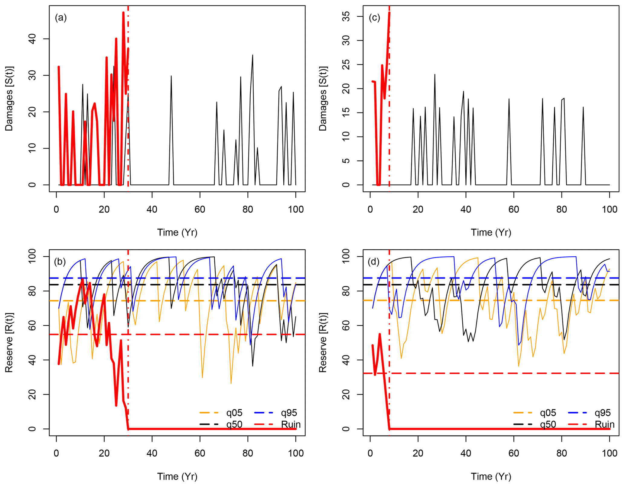
Figure 1 Sample of time series for simulations of S(t) (upper panels) and R(t) (lower panels) with B=0 (isohydric: panels a and b) and B=0.4 (anisohydric: panels c and d). The red lines show sample trajectories of S(t) and R(t) for which R(t) reaches 0 in t<100 years. A vertical dashed-dotted line indicates the ruin time. The black lines indicate trajectories of S(t) and R(t) (for B=0 and B=0.4) that achieve the median of the temporal mean of all 10⁴ trajectories of R(t). The orange and blue lines in panels (b) and (c) show the trajectories of R(t) that achieve the 5th and 95th quantiles of all 10⁴ simulation means. The horizontal dashed lines in the lower panels (b) and (d) represent the means of the represented trajectories before ruin.

Figure 1c and d show the time series of the damage S(t) and reserve R(t) functions for four key trajectories when B=0.4 (anisohydric). The damage function yields the same statistical properties but the scaling is different, so the integrated damage is similar in both cases: the hazard is scaled so that the damage at year t is distributed over t and t+1. For this sample of simulations, the reserve averages for the 5th quantile, median and 95th quantile trajectories are, respectively, 75, 84 and 88 reserve units. These values for the anisohydric strategy are similar to those for the isohydric strategy in Fig. 1a and b. The reserves R(t) with B=0.4 present slightly slower variability for the upper quantiles (the black and blue lines in Fig. 1b and d), which is explained by the memory induced by B>0. The empirical probability of a ruin within 100 years (see Eq. 2) is higher for B=0 ($\mathrm{\Psi }=\mathrm{4}\times {\mathrm{10}}^{-\mathrm{3}}$) than for B=0.4 ($\mathrm{\Psi }=\mathrm{1.5}\times {\mathrm{10}}^{-\mathrm{3}}$). In both cases, a ruin is a rare event for the chosen physiological parameters, and the return period of a ruin (i.e. the inverse of its probability) is larger than 100 years. This justifies our statistical approach of simulating a very large ensemble of trajectories, as the key difference between the tree strategies is a small probability that is difficult to assess from observations.

In principle, a physical evaluation of the model is difficult. The main reason for this is the nature of the phenomenon that is modelled – it does not occur very often. Ruin of insurance companies hardly ever occurs for complete validation of the Cramer–Lundberg model, which could represent a heuristic argument that this model works (at least in that domain of application). In practice, a lot of data have been collected from dead trees and surrounding trees that are still alive to evaluate how dead trees behave in the years before they die (e.g. Villalba et al., 1998; Bréda and Badeau, 2008). Hence, differences in tree ring width between dead and living trees can be considered a good proxy for tree reserves. Cailleret et al. (2017) synthesized data on differential tree growth and used it as a proxy for NSC in various climate hazard scenarios. There is good agreement between our simulated evolution of reserves in the case of ruin (Fig. 1b and d) and the observed evolution of relative tree ring growth before tree death. In particular, Cailleret et al. (2017) show that there is an observed relative decrease in growth between 20 and 50 years before tree death in most cases, which is consistent with our simulations.

3 Data

The goal of this section is to provide climate constraints on the parameters of the hazard function S(t).

3.1 Observations

Meteorological data are taken from the European Climate Assessment and Dataset (ECA&D) database (Haylock et al., 2008). We use daily maximum temperature (TX) and daily precipitation (RR) data from stations in Berlin, De Bilt, Orly, Toulouse and Madrid. This choice is motivated by the desire to cover a large area of Western Europe. We consider data from 1948 to 2019 (>70 years of daily data). Less than 10 % of the values are missing from this dataset.

3.2 Drought–heatwave damage index

We consider the drought–heatwave index I_YV (defined in Appendix A), which is based on precipitation frequency and temperature values from the ECA&D database. This index is computed for five ECA&D stations (Berlin, De Bilt, Orly, Toulouse and Madrid). This new index is considered due to the shortcomings of pre-existing indices that prevent reliable and relevant statistical modelling. On the one hand, the most physically relevant indices are based on soil moisture, but they do not cover a period that is long enough to determine the GPD parameters of its extremes. On the other hand, indices that use well-measured meteorological variables (e.g. temperature and precipitation) are not fully adapted to reflect drought (see Appendix A). This justifies the development of an index from which we can infer the GPD parameters of the damage function due to hazards. The index I_YV yields high values (more than 1.1 ^∘C) during summer drought and heatwave events and low values (less than 1 ^∘C) for wet and cold summers.

From the spring–summer variations of this index, we determine the generalized Pareto distribution parameters of the daily index I_YV when the (daily) values exceed the 95th quantile. As the daily values are temporally correlated (by construction, as the index is a running sum), we consider the maxima of clusters above the 90th quantile and determine the number of days that exceed the 95th quantile threshold. This procedure is advocated in the textbook of Coles (2001).

The values and standard errors of the GPD parameters (threshold, scale and shape) as well as the Poisson parameters for the event duration and return period are shown in Table 1. The values of the GPD parameters are consistent with the existing literature (e.g. Parey, 2008; Kharin et al., 2013).

Table 1 Parameter value ranges for the damage function S(t) obtained from the drought–heatwave (HW) index I_YV values computed for the five stations. The average GPD threshold is the average of the 95th quantiles of the index for the five stations. The average GPD scale and shape parameters are the averages of the estimates for the indices for each of the five stations. The ranges of the GPD parameters take uncertainties into account.

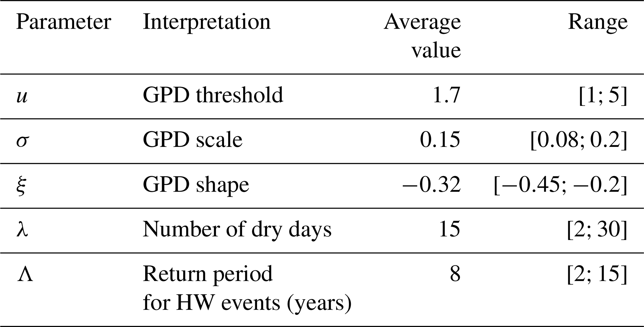
We consider the value ranges in the parameters obtained from the five stations and their uncertainties, and obtain the envelope for each parameter from their lower and upper uncertainties. This provides a conservative estimate of the range of variation for each parameter (i.e. a wide range). Using those ranges of the parameters, we simulate generalized Pareto distributions for the damage function in the model of Eq. (9).

4 Experimental design

The physiological parameters in Eq. (8) are fixed at b=0.25, p₀=25 % yr⁻¹ and R_max=100 (in % of ≈2 kg C m⁻²). We simulate N=10⁶ trajectories of R(t) for 100 years, with an initial condition of R(0)=60. For each trajectory, the parameters of the damage function S(t) are randomly sampled from a uniform distribution with a range that is estimated from the drought–heatwave stress index I_YV (in Sect. 3). The bounds of the uniform distributions are given in Table 1 and reflect the variability across Berlin, De Bilt, Orly, Toulouse and Madrid.

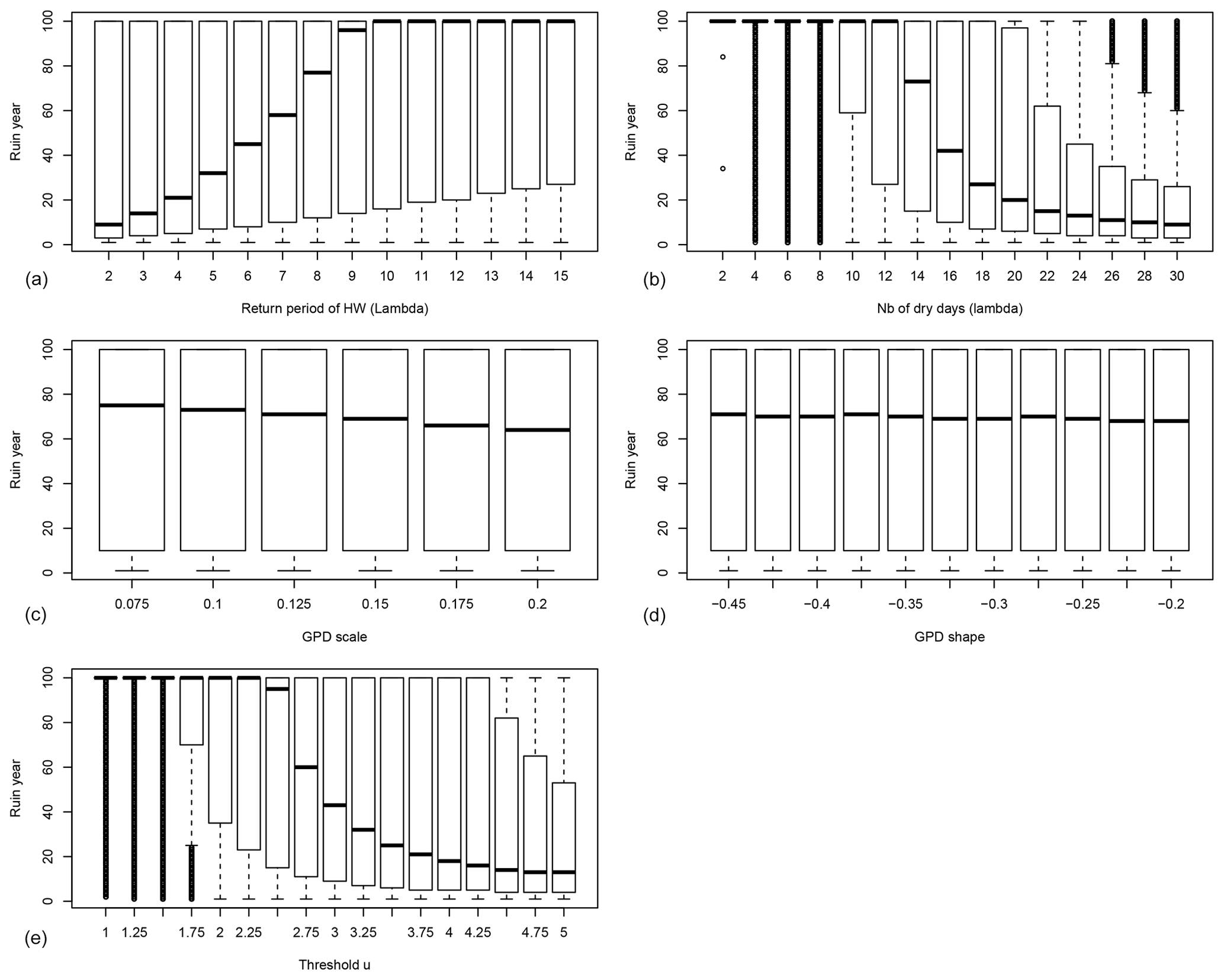
Figure 2 The probability distribution of the ruin year τ as functions of the drought–heatwave (HW) return period Λ (a), the number of days when I_YV exceeds the threshold u during summer λ (b), GPD scale σ (c), GPD shape ξ (d) and the threshold u above which damage S(t) is triggered (e). B=0 in all experiments. For each value of the control variable, a boxplot is given. The thick horizontal bar in each box represents the median (q50) of the distribution. The boundaries of each box represent the 25th quantile (q25) and the 75th quantile (q75). Each upper whisker represents $min[max(\mathit{\tau }),\mathrm{1.5}\times (q\mathrm{75}-q\mathrm{25})+q\mathrm{50}]$. The lower whiskers are $min[max(\mathit{\tau }),q\mathrm{50}-\mathrm{1.5}\times (q\mathrm{75}-q\mathrm{25}\left)\right]$. The small circles represent data that are above or below the whiskers; note that the circles below the lower whiskers tend to be close to each other and therefore appear like thick vertical lines.

From those ensembles of simulation trajectories, we determine the average reserve R(t) before ruin 〈R〉 and the ruin time T_ruin (if it ever occurs). Due to the way in which the model is constructed, R(t) evolves between 0 and 100 (the optimal reserve) and T_ruin is between 1 (immediate ruin) and 100 (no ruin during simulations of 100 years).

The large number of trajectories (10⁶) helps us to investigate the dependence of 〈R〉 and T_ruin on the parameters of S, namely σ, ξ, λ and Λ (see Table 1).

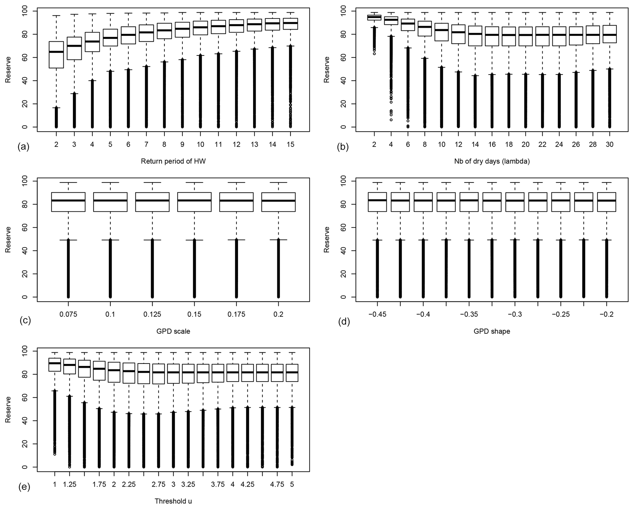
Figure 3 Probability distribution of the average reserves before ruin 〈R〉 as functions of the drought–heatwave (HW) return period Λ (a), number of hot days during summer λ (b), GPD fit scale σ (c), GPD fit shape ξ (d) and the GPD threshold u (e). B=0 in all experiments. For each value of the control variable, a boxplot is given. The thick horizontal bar in each box represents the median (q50) of the distribution. The boundaries of each box represent the 25th quantile (q25) and the 75th quantile (q75). Each upper whisker represents $min[max(\langle R\rangle ),\mathrm{1.5}\times (q\mathrm{75}-q\mathrm{25})+q\mathrm{50}]$. Each lower whisker has the symmetric formulation. Small circles represent data that are above or below the whiskers; note that the circles below the lower whiskers tend to be close to each other and therefore appear like thick vertical lines.

5 Results

The dependence of the ruin time on the four damage parameters when B=0 is shown in Fig. 2. Each boxplot depicts the probability distribution of the ruin time for a given value of one parameter and a random combination of the other parameters.

Figure 2 highlights the fact that the system can shift from a no-ruin state to probable ruin within a century upon making rather small changes to the frequency of extreme days in the index I_YV (either the frequency of dry and hot summers or the number of dry and hot days during a hot summer). The dependence on the scale parameter σ and the shape parameter ξ is rather weak (Fig. 2c, d). The prescribed ranges of variation for those GPD parameters are small in absolute value. The GPD threshold u has an important impact on the ruin time, as the probability distribution of the ruin time shifts from a median of 100 years to a median of 70 years with a 6 % change in the threshold u (i.e. upon changing from u=2.5 to u=2.75; Fig. 2e).

We define that bifurcation of the ruin probability occurs when the median ruin year τ becomes less than 100 years. From this experiment (B=0), we find that a “no ruin to ruin” bifurcation occurs when the return period threshold of 9 years is crossed (Fig. 2). If we focus on the last 20 years in Western Europe, extreme summer heatwaves and droughts occurred in 2003, 2006, 2018 and 2019. This might imply that European forests with trees that yield those physiological parameters are close to the threshold of positive ruin probability.

The threshold number of hot days per summer is 14 d (Fig. 2b). This parameter controls the magnitude of the random sum in S(t) because the daily hazards Y_k yield a bounded tail (ξ<0). This means that if heatwaves can exceed 14 d in duration, tree ruin becomes significantly likely before the end of the 100 years. Such an event occurred in 2018 in Europe (Yiou et al., 2020).

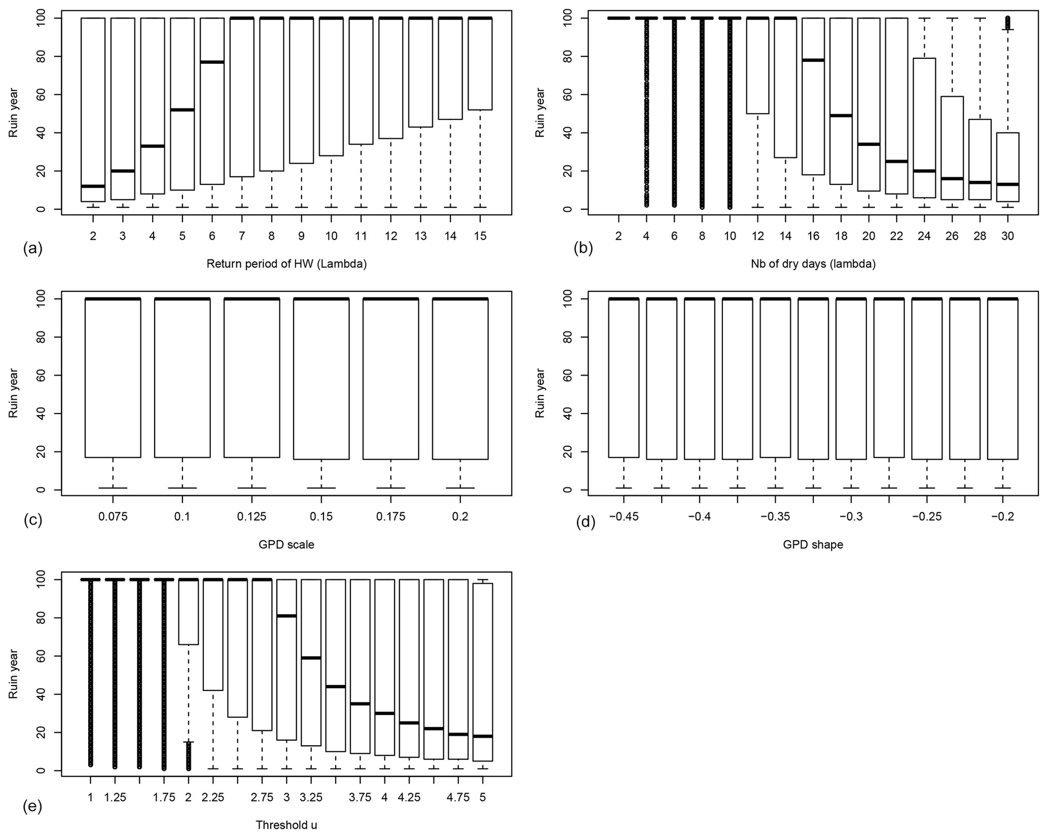
Figure 4 Probability distributions of the ruin year τ as functions of the drought–heatwave (HW) return period Λ (a), number of hot days during summer λ (b), GPD fit scale σ (c), GPD fit shape ξ (d) and the threshold u above which damage S(t) is triggered (e). B=0.4 in all experiments. For each value of the control variable, a boxplot is given. The thick horizontal bar in each box represents the median (q50) of the distribution. The boundaries of each box represent the 25th quantile (q25) and the 75th quantile (q75). Each upper whisker represents $min[max(\mathit{\tau }),\mathrm{1.5}\times (q\mathrm{75}-q\mathrm{25})+q\mathrm{50}]$. Each lower whisker has the symmetric formulation. Data that are above or below the whiskers are shown as small circles; these circles are close to each other and therefore appear like thick vertical lines.

The probability distribution of the average reserves before ruin 〈R〉 for trees with B=0 is shown in Fig. 3. This figure highlights that 〈R〉 weakly depends on the GPD parameters of the damage function (Fig. 3c, d). The average reserves strongly depend on the return period of heatwaves, the number of hot days during heatwaves and the GPD threshold u (Fig. 3a, b, e).

Figure 3a shows that when damage (due to droughts and heatwaves) occurs too often (i.e. the return period of events is short), the trees do not have enough time to build enough reserves to face the next extremes.

The behaviour of tree growth when B=0.4 (anisohydric) is qualitatively similar to its behaviour when B=0 (isohydric) (Fig. 4). The bifurcation threshold is 6 years for Λ, 16 d for λ and a value of 3 for u. This suggests a higher resilience of trees with interannual memory (B>0), as the bifurcations occur for higher values of Λ, λ and u.

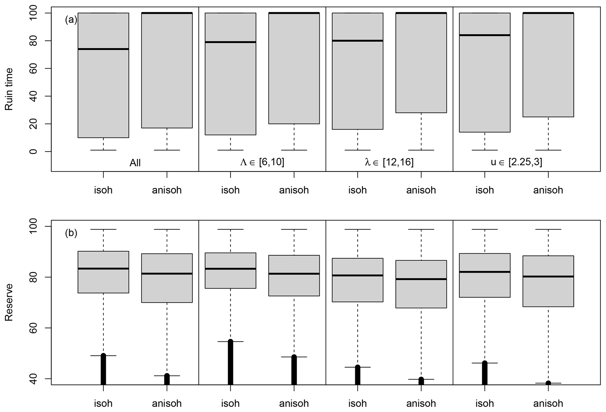
Figure 5 Conditional probability distributions of the ruin time (a) and the reserve (b). The boxplots in the first column (isohydric (isoh: B=0) and anisohydric (anisoh: B=0.4)) are for all simulations. The boxplots in the second column are for drought–heatwave return periods (Λ) of 6–10 years in the isohydric (isoh) and anisohydric (anisoh) simulations. The boxplots in the third column are for drought–heatwave durations during summer (λ) of 12–16 d. The boxplots in the last column are for GPD thresholds of 2.25–3. Data that are below the whiskers are shown as small circles; these circles are close to each other and therefore appear like thick vertical lines.

In a second set of experiments, we maintain the scale and shape parameters constant: σ=0.1 and $\mathit{\xi }=-\mathrm{0.3}$. The other hazard parameters are randomly sampled within the ranges indicated in Table 1. As observed in Fig. 2a and b, the median ruin time τ transitions from 100 years (i.e. ruin is unlikely or does not occur) to <100 years when the event return time Λ is between 6 and 10 years, the event duration λ is between 12 and 16 d, and the GPD threshold u is between 2.25 and 3. Therefore, we focus on the probability distributions of the ruin time and the reserve near these thresholds for the isohydric (B=0) and anisohydric (B=0.4) simulations.

Figure 5 summarizes the probability distributions of the ruin time and the reserve for all simulations and for simulations with hazard values $\mathrm{\Lambda }\in [\mathrm{6},\mathrm{10}]$ years, $\mathit{\lambda }\in [\mathrm{12},\mathrm{16}]$ d and $u\in [\mathrm{2.25},\mathrm{3}]$. On the whole, the probability of ruin Ψ is ≈0.53 for B=0 and Ψ≈0.47 for B=0.4. Figure 5a shows that the anisohydric simulations (B=0.4) yield a larger median ruin time (100 years vs. 74 years for B=0). This means that an anisohydric strategy leads to a longer life expectancy. The differences in the reserve are shown in Fig. 5b. A Kolmogorov–Smirnov test (von Storch and Zwiers, 2001) indicates a significantly higher average reserve for B=0 (83 vs. 81, p-value $<{\mathrm{10}}^{-\mathrm{15}}$). The differences amount to ≈2 units of reserve, which is small compared to the optimal value R_max=100.

On the whole, these results show the dependence of the ruin time on the coping strategy: spreading the damage over 2 years increases the time to ruin in various event scenarios (with different event return times, lengths and intensities). However, the response of the reserve depends on the parameters of the generalized Pareto and Poisson distributions: a higher frequency (or shorter return period Λ) favours isohydric strategies, while the higher intensity (linked to the duration or highest value) slightly favours anisohydric strategies.

6 Conclusions

This paper presents a paradigm based on ruin theory for investigating tipping points for trees using a statistical framework. The framework illustrates how the frequent occurrence of extreme events can fatally damage trees. We described the vulnerability of an idealized forest as its probability of dying through the loss of nonstructural carbohydrate reserves, and illustrated a statistical methodology for identifying climate parameters that control the ruin time. This proof of concept was applied to tree growth, but it could be extended to all types of ecosystems that are vulnerable to climate hazards over long time scales. Careful determination of the physiological parameters of the model from in situ observations is necessary for the operational application of our approach.

The example shown here illustrates how forestry decisions may be guided by a priori information on climate change. The framework shown here takes into account only one type of natural hazard. Others (including storms or fires) could be included, although the recovery rate (or “strategy”) must be specified for each type of hazard.

We have investigated how variations in the hazard parameters affect the damage function and the probability of ruin. The most critical parameters are linked to the frequency of extreme events and their average intensity, which affect the rate of recovery of the trees.

We have examined the impact of strategies to cope with extremes. Although small, this impact has differential effects on the average tree NSC reserve and the probability of ruin. For example, we obtain the counter-intuitive result that, on average, trees with a lower probability of ruin also have a lower average reserve if the hazard frequency changes (Fig. 5). However, if the average intensity of a hazard becomes longer or more intense, trees with a lower probability of ruin also have a (slightly) higher reserve. Hence, changes in hazard intensity or frequency do not have the same effects on isohydric and anisohydric coping strategies, although the differences in effects were found to be small in our experiments.

This subtlety shows that this simple model can yield different kinds of behaviour as a response to hazards. In particular, this emphasizes the need for a proper definition of the hazard (Cattiaux and Ribes, 2018), as this affects the Pareto or Poisson parameters of the hazard-damage function.

This study has obvious caveats. The growth–ruin model used here is exceedingly simple and does not reflect real trees, just as the Cramer–Lundberg model does not reflect the complexity of the insurance sector. The proposed tree model is mainly a proof of concept that could be improved by using parameters or processes with greater physical or biological meaning. A key point of this work is that complex processes which are adversely affected by climatic conditions can be modelled using the Cramer–Lundberg modelling framework, which illustrates the competition between annual regular growth and occasional abrupt damage.

Some of the parameters (especially the impact scale factor A_h in Eq. 9) we used were chosen heuristically. More detailed in situ studies and expertise would be necessary to fine-tune those parameters for each tree species.

Many mathematical papers have described the exact properties of the Cramer–Lundberg model (e.g. see Embrechts et al., 1997, for a review). Our tree growth–ruin model violates some of the simple assumptions of the basic Cramer–Lundberg model, namely the time independence of R(t) in the anisohydric mode. This forbids analytical computation of the ruin time. This is why we resorted to extensive numerical Monte Carlo simulations. Those simulations (≈10⁶ trajectories of 100 years) took less than 4 min on a 12-core computer.

The drought and heat stress index we used is also rather crude and could be refined, although it was only designed to determine the parameters of a Pareto distribution. We then simulated Pareto and Poisson distributions with parameters that were fitted to that index. All simulations were performed with the stationarity assumption (i.e. that the parameters of the GPD distribution do not change over time), albeit with random selections of parameters. Nonstationary simulations could be envisaged as a means to explicitly take climate change into account. Data from climate model simulations could be used to simulate hazards (e.g. Herrera-Estrada and Sheffield, 2017; Massey et al., 2015). This is left to future studies.

Appendix A: Drought–heatwave index definition

As this paper is more a proof of concept for a ruin model than a detailed study (which will be performed later), we consider a simplified drought–heat hazard index that can easily be computed from climatological observations. We are interested in an index that reflects a compound event (Zscheischler et al., 2020) with an extended dry period and high temperatures. There are a few indices of drought or aridity that consider precipitation and temperature (Baltas, 2007). The index of De Martonne (1926) normalizes the cumulative precipitation to the average temperature over a given season:

$$\begin{array}{}\text{(A1)}& I_{\mathrm{DM}}={\displaystyle \frac{P}{T+\mathrm{10}}}.\end{array}$$

Here, the numerator is the cumulative precipitation (in mm d⁻²) and T is the mean temperature (in degrees Celsius). This index was used to determine drought zones. The variation in this index over time can be obtained by considering yearly or seasonal averages of precipitation and temperature. The +10 term in the denominator of Eq. (A1) is included ad hoc to scale the respective variations in precipitation and temperature. Droughts are obtained with small values of this index (low precipitation and high temperature values).

Although easy to compute, this simple index suffers from a few drawbacks. The main one is that it mainly reflects wetness, not drought. Most of its variability is connected with the variability of the precipitation and the upper tail of its probability distribution. Therefore, seasons with little rain produce little variability in the index. One way to circumvent this would be to invert the index (i.e. consider $\mathrm{1}/I_{\mathrm{DM}}$). However, this is still not satisfactory because the values of I_DM for summers with notoriously dry heatwaves (e.g. 1976 and 2003) in Europe are within the average range – they do not stand out, contrary to what is expected (Ciais et al., 2005).

Thus, we propose an alternative drought index, still based on daily precipitation and temperature. For a given day j, we define D_j as the frequency of precipitation, with D_j=0 if precipitation P_j>0.5 mm d⁻¹ and D_j=1 if P_j≤0.5 mm d⁻¹. We then construct an aridity index based on the weighted drought frequency and temperature:

$$\begin{array}{}\text{(A2)}& I_{\mathrm{YV}}\left(t\right)=\sum _{j=t-\mathrm{30}}^t{T}_j\times (D_j+a)A\exp (-(t-j)/\mathrm{30}),\end{array}$$

where t is the time (in days), a≥0 is a scaling constant (similar to +10 in Eq. A1) and T_j is the maximum daily temperature (TX in ECA&D (Klein-Tank et al., 2002)). A≈30 is a scaling constant which ensures that the sum of the exponential weights is 1. In this paper, we chose a=1 after a few tuning tests to verify that the index yields high values during notoriously dry years (e.g., 1976, 2003 and 2018).

This daily index is analogous to the inverse of the De Martonne index. One refinement comes from the exponential weights, which give more importance to recent days than remote days. We can then compute the monthly median, upper quantiles and maximum of I_YV. We compute this index by starting on 1 March, as this is generally when the tree phenology resumes after the winter season at Northern midlatitudes. The daily index is computed until 30 September, when the vegetative cycle is almost finished.

With this new drought index, the extreme droughts and heatwaves of 1976 and 2003 do become exceptional, as expected from the literature (Ciais et al., 2005). Figure A1 compares the precipitation, temperature, de Martonne index and the new index I_YV for temperature and precipitation observations in Orly (near Paris, France). The precipitation or number of dry days does not yield extreme values for years with notorious heat stress in France (e.g. 1976, 2003 and 2019), as they are close to the 25–75th quantile values (Fig. A1b, d). Therefore, the De Martonne aridity index does not yield particularly extreme values for those years (Fig. A1c).

To better evaluate whether the newly defined index is a pertinent indicator of the impact of the climate on vegetation stress, we used the ORCHIDEE land surface model (Krinner et al., 2005) to simulate both soil moisture and tree net primary production (NPP). We performed a simulation using the ERA5 land atmospheric reanalyses at 0.1^∘ × 0.1^∘ resolution (Hersbach et al., 2020) for the gridcell including Orly between 1981 and 2019. After a spin-up of 200 years using the first 10 years of the forcing, the simulation was performed for the entire period. The variations in soil moisture served as input for the hazard function and were a refinement compared to using precipitation only. As an indicator of vegetation damage, we considered the number of days at which NPP is below the 10th quantile (0.15 g C d⁻² m⁻²), which corresponds to the “risk zone” for trees (Fig. A1f).

We found a significant negative correlation between the percentage of dry days and the relative humidity for the 1981–2019 period (Fig. A1c), with $r=-\mathrm{0.7}$ and the p-value $<{\mathrm{10}}^{-\mathrm{6}}$. The NPP variation was significantly (anti)correlated with I_YV ($r=-\mathrm{0.7}$, p-value $<{\mathrm{10}}^{-\mathrm{6}}$). The percentage of days for which NPP was below the 10th quantile corresponded to the percentage of days in which I_YV exceeded a high threshold (Fig. A1e). Therefore, we believe that our decision to use this index has a physical basis, and that it can be used as a proxy to compute the parameters of the damage function.

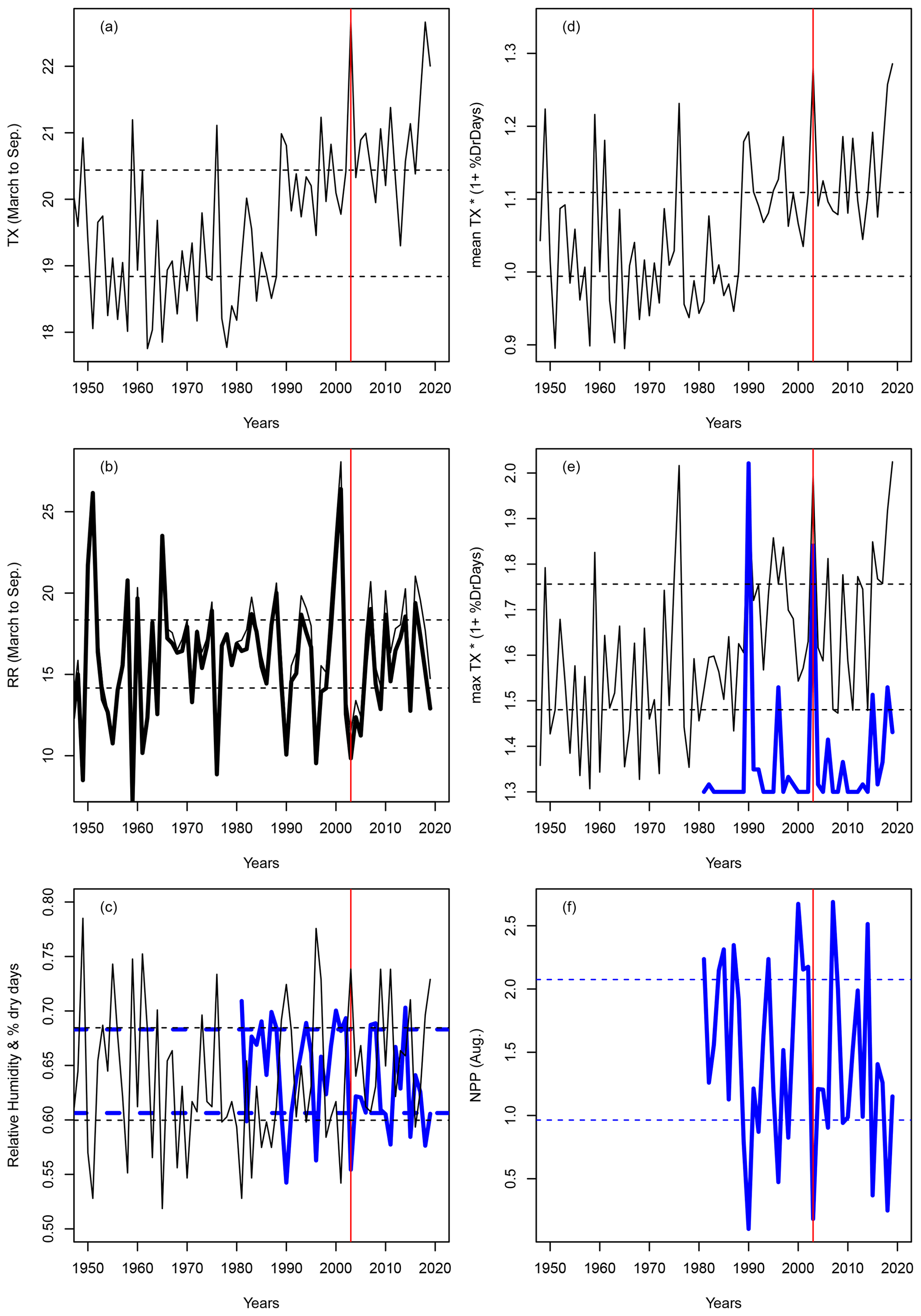
Figure A1 Variations in indices for Orly. Horizontal dashed lines show the q25 and q75 quantiles. The vertical red lines indicate the year 2003. (a) Average (March to September) temperature in Orly. (b) Average (March to September) precipitation in Orly (thin line) and the De Martonne index scaled by 28 (thick black line). (c) Percentage of dry days between March and September (black line) and relative humidity (thick blue line). (d) Mean value of I_YV from March to September. (e) Daily maximum I_YV (black line) and scaled number of days when NPP was below the 10th quantile (thick blue line). (f) NPP variations at Orly, as obtained from an ORCHIDEE model simulation forced by the ERA5 reanalysis.

We computed the index I_YV at five stations – Berlin, Orly, Toulouse, De Bilt and Madrid – from ECA&D (Klein-Tank et al., 2002). Those five stations cover a large part of Western Europe.