the Creative Commons Attribution 4.0 License.
the Creative Commons Attribution 4.0 License.
 | 23 Aug 2021
The potential for structural errors in emergent constraints
Benjamin M. Sanderson
Angeline G. Pendergrass
Charles D. Koven
Florent Brient
Ben B. B. Booth
Rosie A. Fisher
Reto Knutti
Studies of emergent constraints have frequently proposed that a single metric can constrain future responses of the Earth system to anthropogenic emissions. Here, we illustrate that strong relationships between observables and future climate across an ensemble can arise from common structural model assumptions with few degrees of freedom. Such cases have the potential to produce strong yet overconfident constraints when processes are represented in a common, oversimplified fashion throughout the ensemble. We consider these issues in the context of a collection of published constraints and argue that although emergent constraints are potentially powerful tools for understanding ensemble response variation and relevant observables, their naïve application to reduce uncertainties in unknown climate responses could lead to bias and overconfidence in constrained projections. The prevalence of this thinking has led to literature in which statements are made on the probability bounds of key climate variables that were confident yet inconsistent between studies. Together with statistical robustness and a mechanism, assessments of climate responses must include multiple lines of evidence to identify biases that can arise from shared, oversimplified modelling assumptions that impact both present and future climate simulations in order to mitigate against the influence of shared structural biases.
- Article
(432 KB) - Full-text XML
- BibTeX
- EndNote


Models of the climate system face a particular challenge: their primary purpose is to project the future response of the Earth system to forcings that have yet to be realised. Confidence in models' future projections cannot come from iterative verification and improvement but instead must be grounded in a combination of an understanding of the adequacy of simulation of relevant Earth system feedback processes, together with an assessment of the degree to which the models can represent historical behaviour. The latter can potentially provide metrics or constraints that can inform which configurations of each model are most defensible as tools to project future climates.
In climate model development and calibration, these types of constraints are utilised in an extended expert assessment where biases in climatology and historical trends are iteratively reduced and addressed through improved process representation and parameter adjustment (Hourdin et al., 2017; Mauritsen et al., 2012; Schmidt et al., 2017) or systematically through the use of perturbed ensembles and formal inference (Tett et al., 2017; Williamson et al., 2013; Zhang et al., 2018). Adequate performance on a subset of metrics is generally accepted as necessary for consideration as a member of the collection of climate models (Eyring et al., 2016) used to assess future change in IPCC assessment reports (Pachauri et al., 2014); for example, the need for models to conserve energy or to broadly reproduce the observed global mean temperature evolution of the 20th century. Other performance metrics may be of particular interest to specific modelling centres such as reducing biases in the simulation of a particular regional climate or for a particular application (for example, for simulating climate features relevant for energy infrastructure (Golaz et al., 2019) or optimising model performance at high latitudes (Tjiputra et al., 2020)).
Recent literature (Bretherton and Caldwell, 2020; Brient, 2019; Cox, 2019; Eyring et al., 2019; Hall et al., 2019; Klein and Hall, 2015) has also focused on a class of “emergent” constraints that differs conceptually in that the relevance of the metric is defended by the existence of a correlation between a potentially observable metric and a projected future climate response within an ensemble of Earth system model (ESM) simulations. Emergent constraints (ECs) are generally applied in a regression framework, where the ensemble is used to define a predictive relationship that can be combined with observations to produce an estimate of constrained projected values. Examples include constraints of equilibrium climate sensitivity (hereafter ECS) from aspects of natural variability (Cox et al., 2018b) and cloud properties (Brient and Schneider, 2016; Sherwood et al., 2014), transient climate response (TCR) from observed warming trends (Nijsse et al., 2020; Tokarska et al., 2020) and future carbon cycle (Cox, 2019) and ice-albedo feedbacks (Cox, 2019; Qu and Hall, 2007; Thackeray and Hall, 2019) from their observed seasonal variations.
There are a number of recognised factors that might lead to overconfidence in the projections from emergent constraints. The first is that because of the relatively small sample size in CMIP ensembles (or small effective sample size due to model interdependencies; Knutti et al., 2013; Masson and Knutti, 2011; Sanderson et al., 2015) and the large number of outputs, it is inevitable that some variables will be correlated with climate response metrics by chance (Caldwell et al., 2014). This means that our confidence in a constraint cannot arise from correlation across the ensemble alone, but must also include the plausibility of the proposed mechanism that relates the predictor to the future climate response (Caldwell et al., 2018). However, although many published emergent constraints propose a physical explanation for an underlying process that might jointly control the predictor and predictand, robust demonstration of a mechanism often requires tools that are not available, such as systematic sampling of parameters and process representations in models (Hall et al., 2019; Klein and Hall, 2015).
At least some emergent constraints can be shown to be overconfident using existing data by considering new models that are outliers in previously proposed relationships (Klein and Hall, 2015; Schlund et al., 2020) or by the lack of agreement of different constraints on the same quantity in the literature (Brient, 2019). Such disagreement might arise due to inconsistency in the definition of a climate response; for example, if ECS is in fact dependent on the climate state then the value inferred from cooling during the last glacial maximum would differ from that inferred from recent decades. But overconfidence could also arise from overly strong statistical assumptions on the robustness of ensemble-derived relationships (Williamson and Sansom, 2019). The standard regression model uses an ensemble-derived regression relationship between predictor (the potentially measurable variable) and predictand (the unknown climate response) to make a calibrated projection, implicitly assuming the real world is exchangeable with models in the ensemble, which is to say that the relationship is equally likely to apply to the real world as to members of the model ensemble.
It is generally understood that Earth system models, like any model, contain errors and approximations, which means we would not expect this assumption of exchangeability to hold. We know that the models that populate our ensembles are subject to limits of resolution and complexity. This means that they can be considered only as approximations of the real world, likely with more in common with each other than reality (an issue that can be compounded by replicated assumptions and components within the ensemble; Caldwell et al., 2014; Sanderson et al., 2015).
However, although the mean and variance of ensemble projections may be subject to biases, the standard regression model used in ECs makes a strong additional assumption of exchangeability that intra-ensemble relationships are applicable to the real world, potentially leading to a confident yet incorrect constrained projection. Even in the presence of a strong correlation and a plausible physical mechanism explaining the constraint in simulations (Caldwell et al., 2018), the correlation might only arise due to common simplifications throughout the ensemble. Such concerns have led to debate as to whether emergent constraints should be included in integrative assessments of uncertainty in ECS (Sherwood et al., 2020), underlining the need for a robust framework in which to consider emergent constraints as lines of evidence.
A first step towards more robust use of emergent constraints is to combine different lines of evidence (Bretherton and Caldwell, 2020; Brient, 2019), effectively relaxing the assumption that a single constraint is reliable (but maintaining that constraints have some potential value, even if they disagree). However, enacting this approach requires considering additional factors: the degree to which each component constraint has a plausible mechanism (Caldwell et al., 2018) and the degree of independence assumed between different constraints (Bretherton and Caldwell, 2020).
Uncertainties in the relationship and in the source ensemble can at least be represented by framing the problem in a Bayesian framework (Renoult et al., 2020) or using information theory approaches (Brient and Schneider, 2016). These frameworks can naturally allow the integration of multiple constraints by effectively weighting the climate responses of different models in the ensemble by a likelihood informed by a set of constraints; however, these approaches do not test the fundamental implicit assumptions of the regression framework used in most published ECs. Critically, they can also be expanded to represent the likelihood that ensemble members are exchangeable with reality (Williamson and Sansom, 2019), which is effectively assumed in most studies published to date. But even in an ideal case, elements of the calibration of the statistical model parameters would remain somewhat subjective, conditional on prior assumptions about climate responses and chosen metrics of model adequacy and interdependency.
In the following section, we discuss how emergent constraints could hypothetically arise due to structural deficiencies in how processes are represented in the model; a predictor–predictand relationship could exist within the common simplified framework of model parameterisations, which would be overly confident if applied to the real world. To illustrate this, we consider a situation where we know that our ensemble explores only a single model structure that is oversimplified compared to the real world.
Although the concept of emergent constraints as applied to multi-model ensembles has become popular in the last decade, the general formulation was used previously in the perturbed parameter literature. Piani et al. (2005) used a statistical formulation that might today be classified as an emergent constraint, identifying statistical modes of variability that were correlated with climate sensitivity in a large ensemble of perturbed parameter experiments (PPEs) then using observations to produce constrained estimates of ECS. The ensemble used in this case was sufficiently large (Stainforth et al., 2005) that the relationships were statistically robust in sample but were found to be inaccurate when applied to an out of sample set of simulations (in this case, predicting the climate sensitivity of members of the CMIP ensemble Sanderson, 2013).
To understand why this is the case, we must consider the conceptual differences between perturbed parameter and multi-model ensembles. In PPEs, a single model structure is used, and both predictors and predictands are functions of the parameters that are perturbed in the experiment. Emergent constraints in a PPE are generally easy to find (Knutti et al., 2006; Piani et al., 2005; Sanderson, 2011; Yokohata et al., 2010) because there is a low-dimensional functional relationship between predictors and the future response in the ensemble – both are, by construction, functions of the perturbed input parameters. Feedback variation in a PPE is a function of a subset of the parameters that have been perturbed; thus, if any potentially observable quantities are also functions of those same parameters, an emergent constraint is automatically present. Due to this underlying parametric structure, many emergent constraints can be found in a PPE, but they are not individually useful because there are no model versions that satisfy all constraints simultaneously due to the structural component of the model error, which cannot be tuned (Sanderson et al., 2008), and their predictions are generally not applicable to other models (Sanderson, 2011, 2013; Yokohata et al., 2010) (an effect that has been observed in multi-structure PPEs; Kamae et al., 2016).
In model calibration exercises, structural errors in a single model manifest through differences in optimal parameter configurations that arise from prioritising different observations in the cost function. For example, different optimal parameter configurations minimise errors in the Amazon and Indonesian rainforests (McNeall et al., 2016), implying an underlying structural error in the model, which requires that a global calibration must be a trade-off in biases in the two regions, leaving an irreducible error that cannot be eliminated by parameter adjustment alone.
It is understood that probabilistic predictions of future changes made from a PPE must be robust in the face of this irreducible error (Rougier, 2007). In some cases, the multi model ensemble (MME) has been used as an out of sample test to assess overconfidence in predictions made from relationships within the PPE (Sanderson, 2013; Sexton and Murphy, 2012). The correspondence between model errors and the model parameter space also allows for the conceptualisation and quantification of error trade-offs through “history matching” (McNeall et al., 2016; Williamson et al., 2013) (approaches that rule out parts of parameter space that perform poorly in multiple metrics). Such approaches can retain a subset of model variants with comparable net errors but with different trade-offs (in the simple example above, including model versions that minimise errors in either the Amazon or Indonesian rainforests).
Such strategies seek to incorporate model performance in reproducing a range of observables using a model that is imperfect, where it is understood that placing all emphasis on a single observable (as in an emergent constraint) would lead to overconfidence. In a PPE, this is demonstrable because we have a wider structural sample (the MME) in which predictions can be tested and because model errors can be represented as a function of model parameters, which helps us both conceptualise and quantify systematic errors.
In an MME, we do not have similar out-of-sample estimates to illustrate the limitations of ensemble-derived correlations, and there is not necessarily a simple underlying parametric structure that allows us to quantify how assumptions map onto errors. Our experience with PPEs has shown that emergent constraints can arise due to an underlying parametric structure, which is present by construction in a PPE, but may also be effectively present in an MME if the same parameterisations are used throughout the ensemble. This is a potential source of overconfidence in existing ECs that is not generally accounted for.
If an MME includes subsets of models with common structural assumptions, it is also possible that ECs may exist within a given subset. In such cases, confidence in the emergent constraint should be conditioned on the degree to which the models in the subset are plausible. Underlying these uncertainties is a requirement for independently assessing the likelihood or plausibility of model structures.
In short, we cannot easily quantify the impacts of structural error in MME-derived ECs, but it is equally not justifiable to assume that the MME is interchangeable with reality or that common structural errors are absent. Indeed, the very presence of an EC for a given process in an MME might be indicative of a lack of diversity of process representation because constraints are more likely to emerge if there are limited effective degrees of freedom represented in the ensemble. Robust multi-metric approaches that are a demonstrable necessity in a PPE are equally advisable in an MME.
How then do we assess whether an ensemble is sufficiently structurally diverse that an emergent constraint arising from it could be applicable to the real world? In a PPE, constraints can be tested to some extent by testing relationships in the MME, which we can assume contains a larger structural sample; but for an MME, we have no such superset. If an emergent constraint has been found in an MME (providing it has not been demonstrated to be statistically spurious by, for example, additional models that significantly weaken the correlation Klein and Hall, 2015), it then remains to assess the degree to which that emergent constraint can be applied to reality (Williamson and Sansom, 2019).
Here, we propose that ECs can be categorised conceptually into three distinct “kinds” and, by doing so, the nature of their potential structural errors can be better evaluated.
3.1 Constraints of the first kind: bias persistence or signal emergence
The first kind of constraint includes cases where the measured quantity and the unknown quantity are of the same nature, such that both are expressions of a system's response to a forcing with comparable spatial and temporal features. For example, if the observed historical warming in an MME is used to constrain the warming in a future scenario (Jiménez-de-la-Cuesta and Mauritsen, 2019), both predictor and predictand are expressions of global mean warming in response to a gradually increasing greenhouse gas forcing (constraining transient climate response through observed warming (Nijsse et al., 2020; Tokarska et al., 2020) could be argued to fall into this category). Other examples include the conditioning of future sea-ice extent trends on historical trends (Boé et al., 2009; Knutti et al., 2017; Mahlstein and Knutti, 2012), constraining the range of future soil moisture with its observed transient historical trends (Douville and Plazzotta, 2017) and the persistence of carbon dioxide concentration biases in emissions-driven simulations (Hoffman et al., 2014). Similarly, Kessler and Tjiputra (2016) show a relationship between the present day and future uptake of carbon in the Southern Ocean, while Goris et al. (2018) show that similar bias persistence exists for deep ocean carbon uptake in the North Atlantic.
These examples all broadly concern an emergent transient signal in response to a gradual increase in anthropogenic forcing over time, so they are effectively statements that a bias in transient response is likely to persist if forcing continues to increase at the same rate. Because these constraints directly measure the trend itself, they are relatively insensitive to model assumptions in how and why a trend is simulated, provided there exists a robust relationship between the given aspect of future behaviour and its historical trend.
This assumption is valid if it can be defended that both the predictor and projected quantity are describable as functions of the same emerging trend. The resulting EC is effectively a (potentially nonlinear) extrapolation, where the strength of the relationship is conditional on the degree to which models represent similar nonlinearities. The relationship is not strongly conditional on underlying structural assumptions because biases are manifested similarly in the historical and future trends. The strength of the correlation in the EC reflects the degree to which models agree on the form of the extrapolation; thus, the only concern for overconfidence is if the relationship between past and future trends is similarly biased in many models (through the common omission of a state-dependent nonlinearity, for example, or a missing forcing in one period in most models).
Constraints of this type are similar to the classical detection problem (Hegerl and Zwiers, 2011; Ribes et al., 2017) where the amplitude of an emerging signal in response to a forcing is estimated in the presence of noise arising from internal variability and other confounding forcers. There exists a large literature in performing such detection of a signal response to a forcing in the context of noise, model errors and other confounding forcings (Hegerl and Zwiers, 2011).
3.2 Constraints of the second kind: process isolation
The second kind of EC involves the identification of a primary mechanism that governs the future response and the subsequent proposal of an observable quantity that constrains the strength of that feedback within the ensemble. There are a large number of ECs that fall into this category for ECS (Brient et al., 2016; Lipat et al., 2017; Sherwood et al., 2014; Siler et al., 2018; Su et al., 2014; Tian, 2015; Trenberth and Fasullo, 2010; Volodin, 2008; Zhai et al., 2015b), in most cases involving mechanistic constraints on the response of shallow convective clouds to warming (considered to be the primary source of uncertainty in ECS in CMIP5 (Andrews et al., 2012) and CMIP6 (Zelinka et al., 2020)). Other studies propose to directly constrain individual cloud feedbacks (Brient et al., 2016; Gordon and Klein, 2014; Qu et al., 2014; Siler et al., 2018) or future precipitation changes (Allen and Ingram, 2002; Watanabe et al., 2018). In the ocean, similar process-based constraints were proposed in Terhaar et al. (2020), which found a relationship between ocean acidification and Arctic deepwater formation, which was in turn related to present day Arctic surface water densities.
Emergent constraints obtained by statistical data mining (either transparently or otherwise) can potentially fit into this category, though in order to be defensible, such constraints must be demonstrated to be statistically robust (Caldwell et al., 2014) and also provide a plausible mechanism to explain why the candidate process is the dominant factor in explaining ensemble variance in the future response and why the proposed observable is an expected metric of that process (Caldwell et al., 2018; Hall et al., 2019).
However, unlike constraints of the first kind, a process-based constraint does not describe uncertainty in the future response in a general sense – at best, it describes the leading order process, which explains variability in the future response across the ensemble. A plausible, robust, process-based EC is still conditional on the plausibility of the relevant process as it is represented in the class of models used in the ensemble. However, confidence in process representation can be assessed and potentially increased through consideration of plausibility of common model assumptions (Klein and Hall, 2015) or identification of independent observables that can be used to assess the degree to which models represent relevant processes (Terhaar et al., 2020).
3.3 Constraints of the third kind: frequency substitution
The third kind of constraint proposes that the future response to a given forcing represented by the variable A can be constrained using the response of the system to a different forcing represented by the variable B, the response to which is potentially observable. Unlike constraints of the second kind, this logic does not require a specific feedback mechanism. Unlike constraints of the first kind (a special case), it is also not a priori true that the response of the system to one forcing B is controlled by the same processes that control the future response A. There are thus a larger number of potential sources of structural error compared to the first kind of constraint, as the simulation of responses to both A and B may have ensemble-wide biases and missing components. In this case, those potential biases may arise only in the simulation of the predictor or only the predictand, and so errors have the potential to weaken the constraint.
In such cases, the forcing associated with B differs from A in terms of its timescale or mechanism. Examples of this third kind of constraint have taken B as the seasonal cycle (Covey et al., 2000; Knutti et al., 2006; Zhai et al., 2015b), the inter-annual variability simulated by the models (Cox et al., 2018b; Masson and Knutti, 2013a) (though it is arguable whether such unforced variability is in-fact measurable; Rypdal et al., 2018) or the response to paleoclimate forcings (Hargreaves et al., 2012; Hegerl et al., 2006; Royer et al., 2007; Schmidt et al., 2014) or volcanic events (Boer et al., 2007; Plazzotta et al., 2018; Wigley, 2005). Similar approaches have used the seasonal cycle in snow albedo to constrain sea-ice trends (Qu and Hall, 2014), future extreme precipitation (O'Gorman, 2012) and vegetation carbon responses to warming (Cox et al., 2013; Wang et al., 2014; Wenzel et al., 2014). Kwiatkowski et al. (2017) found that the sensitivity of tropical ocean productivity to internal variability driven temperature change was related to future changes in productivity under anthropogenic global warming. The concept can be taken further by using tendencies of forecasts on a timescale of hours to constrain long-term responses to climate change (Palmer, 2020; Rodwell and Palmer, 2007).
Because our confidence in the EC arises partly from the existence of the correlation within the ensemble itself, we must carefully assess the possibility that the emergent relationship arises due to common assumptions that are deployed throughout the ensemble. Furthermore, it is more likely that a relationship will emerge if the common assumptions are simple, with a small number of effective degrees of freedom in calibration (see Fig. 1 in the simple-model example that follows).
For example, many CMIP-class models use similar temperature-scaling assumptions for soil respiration (Shao et al., 2013). There is evidence that the majority of soil carbon stocks in the CMIP5 archive can be explained by a reduced order function of soil temperature and plant productivity, which notably fails to reproduce observed carbon stocks (Todd-Brown et al., 2013), implying a common structural bias. A constraint on the future temperature response in CMIP (Cox et al., 2013) could be argued to effectively be a calibration of a low-order soil respiration model.
In such a situation, where the CMIP models have a common and/or low-order structure differing only in their calibration, the MME is in fact a PPE in disguise. Our assumption that the ensemble represents a complete set of plausible structural variants interchangeable with reality is far from the truth, and, worse, an ensemble with such structural limitations is more likely to produce constraints of the third kind (as we see in the simple example that follows) because the response to any forcing is effectively governed by a small number of degrees of freedom. Although there may be a robust intra-ensemble relationship between the response to a short-timescale forcing and a long-timescale forcing, this relationship may be the direct product of a simple common structural framework. In order to have confidence in the constrained projection, it is then necessary to assess whether that common framework is both adequate and the only plausible mechanistic model for the process.
It should also be noted that these kinds of constraint might be potentially useful in an illustrative sense but they are not absolute. Some published constraints undoubtedly have elements of more than one type. For example, Zhai et al. (2015b) report elements of both the second and third kinds of constraints in that it isolates a primary long-term feedback process and constrains it using the response to short-term forcing (seasonal variability in this case). Another example is constraining the transient climate response from observed warming (Knutti and Tomassini, 2008; Nijsse et al., 2020; Schurer et al., 2018; Tokarska et al., 2020), which has elements of the first and third kinds of constraints. The transient warming response to an idealised forcing is constrained with its response to historical emissions, which is the first kind of constraint, but there are also conceptual differences between these forcing pathways (most notably the presence of transient aerosol forcing in the real world) and the resulting dominant feedback processes, which introduce elements of the third kind of constraint. Ultimately, the greater the differences between the forced response considered in the constraint and that measured in the predictand, the more the constraint itself depends on the structural assumptions present in the ensemble.
We can illustrate these concepts using ensembles created from two different classes of a simple climate model.
4.1 Heuristic model structures
4.1.1 Single-layer model
The first model uses a single timescale of response, corresponding conceptually to an ocean represented by a single thermodynamic slab:
where C is the heat capacity of the Earth system, T′ is the global mean temperature anomaly, F is the time-dependent climate forcing and λ is the climate sensitivity parameter.
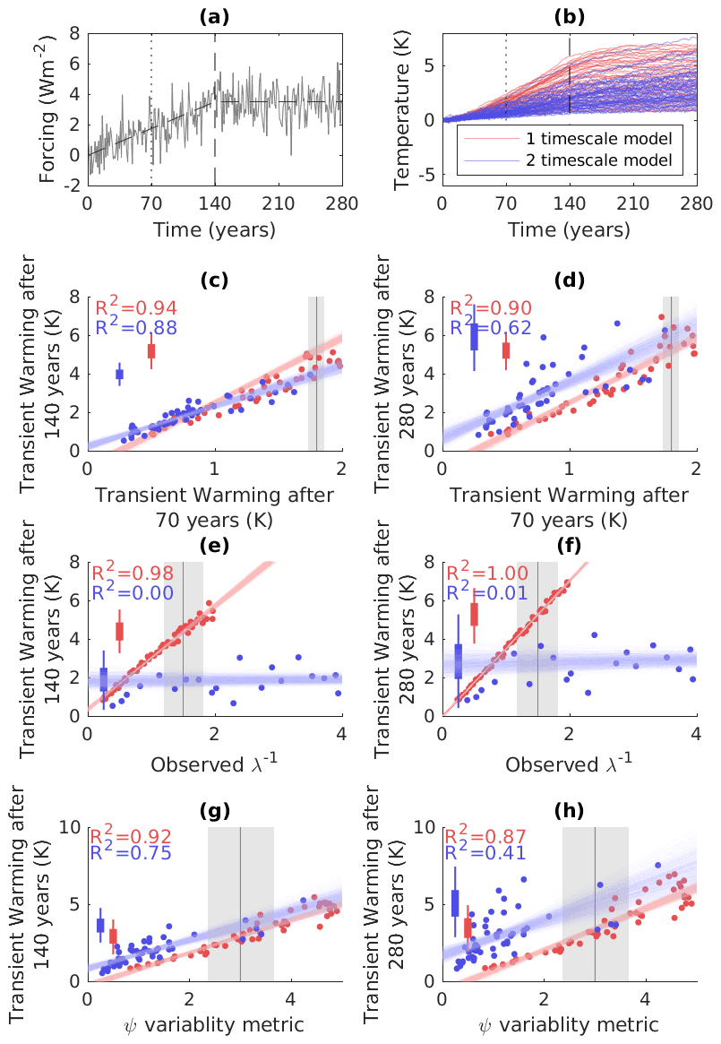
Figure 1An illustration of the three kinds of emergent constraint in two structurally different ensembles. (a) An idealised forcing time series used for each of the simulations – a (noisy) linear ramping of radiative forcing from years 0–140 followed by (noisy) constant forcing from years 140–280. Panel (b) shows the response in 50-member perturbed parameter ensembles of two energy balance models with one (red) and two (blue) timescales of response. (c) A constraint of the first kind showing TCR (warming after 70 years of 1 % annual increase in CO2 concentrations) as a predictor of T140 (warming at time of CO2 quadrupling, 140 years in the same experiment). (d) Warming after a further 140 years of constant (quadrupled) CO2 concentrations. (e, f) Constraints of the second kind using the feedback parameter “lambda” to predict warming after (140, 280) years. (g, h) Constraints of the third kind using a variability metric (Cox et al., 2018b) derived from detrended temperature time series in years 1–70 as a predictor warming after (140, 280) years. In each case, coloured points show members of the model ensemble, lines show bootstrap regression estimates, and grey vertical bars show the 10th, 50th and 90th percentile of the (hypothetical) observed uncertainty distribution. Coloured box and whisker plots show the th and th percentiles illustrating the prediction interval from each ensemble. Variance explained by the predictor for one- and two-layer models is printed in red and blue text respectively.
4.1.2 Two-layer model
The second model is slightly more complex, with the addition of a deep ocean layer (Geoffroy et al., 2013):
where C0is the heat capacity and is the temperature anomaly of a deep ocean layer, γis the thermal diffusion coefficient of heat exchange between the two layers, and ε is the efficacy of heat transfer to the deep ocean (see Geoffroy et al., 2013).
4.2 Idealised experiments
We conduct an idealised climate change experiment where for the first 140 years, CO2 concentrations are increased by 1 % each year resulting in a gradual linear increase in forcing over time, followed by an equilibration period:
A transient component of the forcing is provided by the first term, where a= 0.05 (corresponding approximately to the 1 % CO2 ramping experiment), and a random component is provided by the second term, where η(t) is white Gaussian noise scaled by the factor b= 0.5. In the second 140 years, the transient component of the forcing is held constant:
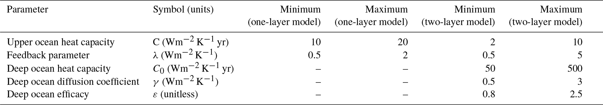
With each model, we produce a range of responses by creating an ensemble with parameters sampled in Latin hypercube: in the first case [Cλ] and in the second case [CCoλεγ]. Finally, we consider how different types of artificial “observation” would constrain the projected response. Parameter ranges for the two-layer model are informed by (Geoffroy et al., 2013) and manually adjusted in the one-layer model to produce a comparable range of transient warming after 140 years (T140 hereafter; see Table 1).
Table 1Parameters used in the one- and two-layer models in the idealised example, and the upper and lower bounds of the sampling range used in the ensemble construction.
In these simple models, we can test constraints of different types and illustrate their sensitivity to common structural differences between the two ensembles. We consider three constraints for the future response in each of these models and then interpret their relative skill.
A constraint of the first kind can be created by using the transient warming observed after 70 years (T70) to predict T140. In this example, the EC exists in both ensembles (though its slope differs a little between the two ensemble types). Transient warming is near-linear in time in both cases, so behaviour at year 140 can be extrapolated from years 1–70. However, for the case of warming at 280 years (T280, i.e. an additional 140 years after forcing is stabilised), we see a strong relationship between T70 and T280 only in the single-layer model (Fig. 1d). In the two-layer model, the temperature response in the first 140 years of linear forcing increase is a combination of both slow (deep) and fast (shallow) timescale components, and transient warming at year 70 can be extrapolated (even if we do not know the relative contribution of the slow and fast components of the warming). However, when the forcing stabilises at year 140, the shallow component quickly saturates and the remaining warming is due to deep ocean equilibration alone. Thus, this additional degree of freedom (shallow vs. deep contribution to transient warming) is unconstrained and T70 is a worse constraint on T280. The one-layer model does not have this additional degree of freedom; thus, T70 is a good constraint on T280 but only because of the structural simplifications present in the model. Because the nature of the forcing differs between the transient and equilibrium stages of the experiment, the constraint of T280 using T70 is a constraint of the third kind in our classification system.
We can consider a constraint of the second kind by assessing how independent data constraining a parameter in the models would constrain its projections. In Fig. 1e, f we illustrate how knowledge of the λ parameter would act as a constraint in two ensembles (as a proxy for information about physical processes in CMIP-class models). In the single-timescale model, λ acts as a near-perfect predictor of warming after 140 and 280 years, and constraining ensemble spread using that parameter would have a large effect. In contrast, in the two-timescale model, the correlation is weak. Although the lambda parameter controls feedbacks (and equilibrium response) in both models, transient response in the two-layer model is strongly governed by deep ocean heat uptake. We know that heat uptake by the deep ocean is an important mechanism for Earth's warming in transient scenarios (Geoffroy et al., 2013), so we have introduced a common structural flaw in models that do not account for the role of the deep ocean. That flaw allows for an apparently strong EC in the single-timescale model ensemble, which is not present in the more realistic ensemble.
The one-layer model ensemble samples a similar range of transient warming as the two-layer model in the first 140 years. For some applications, the one-layer model may be sufficient to model further transient warming, but the strength of an EC based on λ depends on the over-simplistic structure of the one-layer model, which leads to a demonstrably overconfident result in this case.
We can also construct a constraint of the third kind such as the ψ variability metric similar to that used by Cox et al. (2018b), where the variance and lag covariance of temperature variability is used as a predictor of climate sensitivity (though there are conceptual differences to Cox, 2018, given that our model does not have an internal source of noise). In this case, in Fig. 1g, h we consider the ψ metric as a predictor of T140 and T280 in our two ensembles. Once again, the metric is a strong predictor for both T140 and T280 in the one-layer ensemble. Meanwhile, in the two-layer ensemble, the correlation with T140 is weaker (with a different slope to the one-layer case). There is little to no correlation between T280 and ψ. As with the first kind of constraint, both the EC relationship slope and its strength as a predictor depend on common structural assumptions, with a stronger apparent relationship in the ensemble with fewer degrees of freedom.
In these simple examples, we can understand EC behaviour in the context of the model assumptions. Both model types can produce similar transient evolution until forcing is fixed but then the responses diverge, revealing very different equilibration behaviour (see Fig. 1b). The single-layer model equilibrates to a change in forcing over 1–2 decades (depending on the exact choices of C and λ), so that after 140 years most of the response to the forcing experienced to date has already been realised in the model temperature response and little additional warming is subsequently seen. T70, T140 and T280 are all (to first order) controlled by the λ parameter. On the other hand, the two-layer model does not fully equilibrate to a step change in forcing for centuries, so the transient response to forcing, which defines T70 and T140, is controlled by both λ and the deep ocean heat uptake parameters (Coεγ). In this model, neither T70 nor λ are singularly informative about how the model equilibrates.
This illustrates a key issue with the emergent constraint framework: if one has access only to the one-layer model ensemble, one would conclude that λ or T70 are strong emergent constraints on T280, and the strength of the relationship might be used as evidence for the physical plausibility of the EC. But instead, in this case, the strength of the relationship is indicative that the single-layer model is lacking (in this case a deep ocean), and the parameters of the shallow ocean have been adjusted to compensate for this bias in reproducing observed transient behaviour. Furthermore, if independent data on the real-world value of λ was available and used to constrain the response of the single-layer model (and the real world was in fact more appropriately modelled by including the deep ocean), the resulting constrained prediction would be precise but inaccurate because that prediction would be conditional on a common structural assumption that is incorrect.
More generally, the strength of an emergent relationship must be considered in the context of the degrees of freedom that are varied in the ensemble being considered. In the simple example considered here, the historical forced response can act as a constraint on the future response because the forcing term is held constant across the ensemble. In CMIP, the presence of uncertainty in the forcing time series due, in large part, to uncertain aerosol effects render historical warming a poor constraint on future warming (Forest et al., 2002; Knutti et al., 2002) due to compensating forcing and feedback terms in ensemble members (Kiehl, 2007; Knutti, 2008), except in cases where the aerosol forcing term is relatively constant over the time period considered (Nijsse et al., 2020; Tokarska et al., 2020) or additional information is included to disambiguate the responses to different forcings (Allen and Stott, 2003; Hegerl et al., 2000; Kettleborough et al., 2007). In effect, this suggests that the long-term historical warming in CMIP is not a useful constraint because it has already been “used” by model developers who consider reproducing historical warming to be a necessary condition for acceptability of a released model, leading to an ensemble that is converged on the observed global mean historical temperature record but with a range of trade-offs in forcing and net feedback.
Clearly, the models in the example above are vastly simpler than those used in CMIP, but these examples illustrate relationships that could emerge in those more complex models and how they might be incorrectly utilised. Such errors could occur in CMIP-derived ECs if there are processes that are parameterised in a common, overly simplistic fashion across the ensemble. Furthermore, irrespective of increasing model complexity, it is likely that this argument could always be made – one could always imagine a more complex or complete model than the standard at any given time. In this context, a single EC will continue to be at best a conditional statement that could be proved inaccurate or overconfident by the following generation of models.
But for the increasing body of ECs that have been published using CMIP data, how concerned should we be about overconfidence due to common structural errors? This question does not replace the credibility tests that have already been proposed in the literature (Caldwell et al., 2018; Hall et al., 2019): robustness to change in ensemble samples, plausibility of mechanism and evidence of the mechanism and feedback variability from supporting model diagnostics. But for ECs that appear to pass these tests, an assessment of the underlying model assumptions is then necessary. Here we assess a small number of ECs as case studies and how their applicability is to some degree conditional.
5.1 Persistent bias of CO2 concentrations
We consider first an example of an EC of the first kind (Hoffman et al., 2014), which uses the present day carbon dioxide concentration to constrain future carbon dioxide concentrations. Their primary finding is that a historical bias persists into the future in a transient emissions scenario. This exploitation of bias-persistence might be overconfident if the CMIP5 models were missing or misrepresenting key land surface or ocean processes that might differently alter future and historical CO2 concentrations.
The net carbon uptake by the Earth system represents the combined contributions of land and ocean components with greater agreement in models on the net effects than the constituents (Friedlingstein et al., 2014). In the ocean, there is evidence of common biases in CMIP5, for example, in mixing and the uptake of carbon in the Southern Ocean (Sallée et al., 2013). If such biases are compensated through other parameters in order to improve global estimates of net ocean carbon uptake, then ensemble-derived relationships between past and present carbon uptake have the potential to be biased by common errors in the Southern Ocean (Terhaar et al., 2021).
In the land surface representation, there are a number of processes missing from a subset or the entirety of the CMIP5 ensemble. For example, nitrogen limitation was implemented in only one model in the CMIP5 generation of models (Zaehle et al., 2015), where it was found to have the capacity to significantly alter land carbon uptake. For an emergent constraint exploiting the persistence of a CO2 concentration bias, this is potentially an issue if nitrogen availability is not currently limiting but becomes a limiting factor in a future state. A larger fraction of CMIP6 models include nitrogen limitation with diverse implementations. Nitrogen was not found to strongly influence historical carbon uptake but a future effect has not been explicitly ruled out by studies to date (Davies-Barnard et al., 2020), so a repeat of the Hoffman study would be a useful test of the robustness of the EC to a significant structural change between the CMIP5 and CMIP6 generation of land surface models.
There remain a number of additional processes that could potentially influence future carbon uptake that are not comprehensively implemented. Phosphorus limitation has potentially large impacts on the future Amazonian carbon sink (Fleischer et al., 2019) and is absent from CMIP5 models but present in a small subset of CMIP6 models (Arora et al., 2020). The impact on the carbon sink of potential changes in tree mortality in response to CO2 and forest productivity is both critical and absent from CMIP6 class models (Brienen et al., 2020; Needham et al., 2020), as are complex fire–vegetation feedback processes (Teckentrup et al., 2019), diversity in responses to drought (Fisher et al., 2010; Levine et al., 2016; Longo et al., 2018; Sakschewski et al., 2016), vegetation damage under unprecedented heat extremes (Teskey et al., 2015), wind events and pathogen damage (McDowell et al., 2018). These all have the potential to introduce climate–vegetation feedbacks that are currently not represented in the CMIP6 ensemble.
Thus, our confidence in the persistence of the models' present day CO2 bias persisting into the future is reduced because there are processes that are potentially highly significant and are broadly absent from current generation models. However, the nature of a constraint of the first kind means that the integrative carbon cycle response is used as both predictor and predictand, so this kind of constraint could remain robust as long as structural omissions had similar effects on CO2 concentrations in the past and the future. In short, it is a filter on models that have been accurate thus far in simulating the quantity we are ultimately interested in measuring – an arguably necessary (but not sufficient) condition for projecting that quantity into the future. Because the net carbon feedback is being constrained directly, the method is (somewhat) insensitive to the representation of processes that make up that feedback.
5.2 Historical constraints on soil–carbon temperature relationships
We next consider the study by Cox et al. (2013), which relates tropical land carbon uptake–temperature feedback and the historical relationship between the growth rate of atmospheric CO2 and tropical temperature anomalies. Other studies (Chadburn et al., 2017; Varney et al., 2020) have considered similar relationships using spatial variability as a predictor. In CMIP5 models, this constraint (of the third kind) was very strong (Cox et al., 2013). In this case, the focus on the carbon–temperature component of the total carbon feedback isolated the effect of soil respiration temperature response, which in CMIP5 dominates both the predictor and the predictand for the EC. Our confidence in the EC thus firstly depends on whether soil respiration is represented in a common, oversimplified fashion in the CMIP5 ensemble. Independent studies have found that inter-model differences in soil carbon uptake are dominated by the parameterisation choices for soil heterotrophic respiration rather than structural differences (Todd-Brown et al., 2013) and that a lack of ability to represent grid-scale variation in soil carbon levels indicates the potential missing processes. Non-coupled models representing higher levels of microbial complexity and vertical resolution suggest that CMIP-class models may be underestimating the range of potential future soil carbon uptake (Shi et al., 2018).
In CMIP6 models, there remains indication that spatial variability continues to provide predictive information on future soil carbon dynamics (Varney et al., 2020), but the role of soil respiration in the total carbon–temperature feedback is less dominant (Arora et al., 2020), with vegetation productivity responses also playing a role in the ensemble variance. This increases the structural diversity of the relevant model components and has the potential to weaken the strength of the CMIP5 correlation. A repeated analysis of the method of Cox et al. (2013) for the CMIP6 ensemble would therefore be of interest for testing whether the correlation remains equally strong in CMIP6.
5.3 Constraints on future ocean carbon uptake
There exist a number of studies that have considered relationships between aspects of present day and future ocean circulation. Kessler and Tjiputra (2016) propose a constraint between the contemporary and future uptake of carbon in the Southern Ocean, which in the framework laid out here would be recognised as a constraint of the first kind: a trend or rate observed today persists into the future. The Southern Ocean carbon uptake is conditional on both physical and biological model assumptions, and there are potential common CMIP biases in Southern Ocean mixed layer depths (Sallée et al., 2013) and seasonal sea surface temperature (SST) cycles and models with compensating biases in productivity (Mongwe et al., 2016). However, as discussed in Sect. 3.1, such trend extrapolation constraints can remain robust to such compensating biases in the absence of nonlinearities.
Goris et al. (2018) also constrain future oceanic carbon uptake, identifying that models that more efficiently mix carbon down into deeper layers in historical climate continue to do so in the future (a constraint of the first kind) and that such models show a larger seasonal cycle in North Atlantic shallow ocean carbon concentrations due to summer productivity and winter mixing of carbon into the deep ocean (a constraint of the third kind ). The process identification and multi-metric constraint potentially add robustness to this approach, but the constraints remain subject to potential common misrepresentation of ocean biota in the ensemble, such as the common underrepresentation of winter North Atlantic productivity in all CMIP models shown by Goris et al. (2018) and common underestimation of Atlantic meridional overturning circulation variability (Yan et al., 2018), both of which have the potential to bias the simulated seasonal carbon concentration anomalies as well as the derived emergent relationship slope.
Kwiatkowski et al. (2017) identify a strong relationship between the long-term sensitivity of tropical ocean primary production to rising equatorial sea surface temperatures and the interannual sensitivity of primary production to El Niño–Southern Oscillation (ENSO)-driven SST anomalies – a classical constraint of the second kind where the sensitivity of ocean biota temperature variation arising from natural variability is used to infer knowledge about the response to future warming. Such a relationship identifies that the parametric dependencies of tropical productivity are similar for long-term warming and internal variability but, once again, conclusions are subject to potential errors in assessing observed productivity (Stock, 2019) as well as common biases in the effect of the resolved scale on productivity (McKiver et al., 2015).
5.4 Constraining transient climate response with observed warming
The constraint of TCR detailed by Nijsse et al. (2020) (and also Tokarska et al., 2020) use observed transient warming as a predictor of future warming. In this case, the EC falls into the constraint of the first kind category – the predictor and predictand are conceptually similar in that they both represent the transient global mean warming response to a CO2 forcing that is monotonically increasing at broadly comparable rates – but there are differences in terms of the forcing magnitude (present day CO2 levels are less than the double pre-industrial level used in the formal TCR definition) and due to other forcing terms, for example, aerosols and land use change. The authors minimise the role of aerosol forcing changes by considering a time period (1975 to 2013) in which there is relatively constant global mean aerosol forcing, leaving a time period in which greenhouse gas forcing changes are dominant.
The strong correlation in CMIP6, if used as a constraint, tends to rule our upper end of the CMIP6 TCR range (values of 2.3 K and above). This observed warming constraint does not rule out high values of ECS to the same degree (Tokarska et al., 2020), potentially because models exhibit feedbacks on different timescales that are evident as models reach equilibrium in response to a step-change forcing (Rugenstein et al., 2020). However, in response to transient forcing, CMIP models tend to uniformly exhibit near-linear warming trajectories (Gregory et al., 2015), differing only in the temperature growth rate and thus making a strong constraint with effectively one degree of freedom. However, the CMIP5 ensemble indicates a weaker and more noisy relationship between observed warming and TCR, and combining the two ensembles leads to a weaker overall correlation in Tokarska et al. (2020). Until the origins of these differences are better understood, the application of the CMIP6 EC to rule out higher values should be treated with caution.
The TCR metric is, by construction, insensitive to carbon cycle dynamics and aerosol forcing plus potential “tipping points” (Lenton et al., 2019) if they are unrepresented in current generation models. TCR is also a combined function of climate feedbacks and ocean heat uptake dynamics, and models that share the same value of TCR can have different warming trajectories long after forcing levels stabilise (Sanderson, 2020). As such, inter-timescale relationships (such as those between TCR and warming in the last 30 years) are conditioned on the breakdown of composite feedback timescales in the ensemble. If the ensemble variance in TCR is attributable to varying fast timescale processes, this may result in a different slope than if slow timescale processes were varied.
As such, observed warming does not itself constrain equilibrium or post-2100 warming under mitigation (Sherwood et al., 2020), where large uncertainties in the interplay between ocean circulation dynamical responses to warming (Rose and Rayborn, 2016), nonstationary climate feedbacks (Rugenstein et al., 2020) and long-term carbon feedbacks (Koven et al., 2021) are areas of active research.
5.5 Process-based constraints on climate sensitivity
Here, we consider an example of a process constraint of the second kind (Sherwood et al., 2014) on equilibrium climate sensitivity in CMIP5 – though the arguments would be equally applicable to other plausible process-based constraints (Brient et al., 2016; Brient and Schneider, 2016; Zhai et al., 2015a). Sherwood proposes two indirect metrics of lower tropospheric mixing that are related to future reductions in boundary layer clouds (the cloud feedback, which is itself the largest component of inter-model spread in ECS Pincus et al., 2018). The postulated physical mechanism is that models with larger boundary layer mixing will experience stronger ventilation of moisture from the lower troposphere as the atmosphere warms and humidity increases, so these models ultimately experience the most extreme loss of boundary layer clouds. Independent studies have assessed the Sherwood constraints to have a plausible mechanism, with correlated warming patterns occurring in regions that are consistent with the constraint (Brient, 2019; Caldwell et al., 2018). Together with the relatively strong correlation proposed by Sherwood, this makes the study one of the more compelling examples of a physical constraint on ECS in a multi-model ensemble.
If indeed the constraint proposed by Sherwood et al. (2014) is a robust predictor of ECS within CMIP5, the structural robustness of the constraint concerns the degree to which CMIP5 is a representative sample for comparison with reality. This question can itself be divided into three questions: (1) is the process itself sufficiently well represented in CMIP5 to be informative, (2) are there other processes that are absent, undersampled or commonly misrepresented in CMIP5 models that might bias ECS and (3) are there common structural biases that might impact the predictors – the mixing proxies in this case – thus biassing the conclusion of the constraint?
For the first question of boundary layer process accuracy, there is a structurally rich selection of boundary layer schemes in CMIP5 (Edwards et al., 2020), which reduces the chance that the EC is a product of structural homogeneity in the ensemble. There is, however, some evidence that there exist ensemble-wide climatological biases in the current generation of models that can be attributed to common boundary layer mixing structural errors in CMIP5 (Wei et al., 2017). Most CMIP5 generation models rely on low-order turbulence closure schemes that assume, to some degree, a representative length scale for temperature and wind gradients based on Monin–Obukhov similarity theory (Monin and Obukhov, 1954), often complemented by bulk convection schemes or energy closure arguments to resolve remaining boundary layer mixing. The testing of the persistence of the EC in CMIP6, which includes models with higher order closure schemes that do not make this explicit assumption (Bogenschutz et al., 2018), thus broadens the diversity of representation of boundary layer mixing in the ensemble and creates a useful test of structural robustness for the CMIP5 era constraints.
The second question relates less to the representation of the process in question (shallow convection and boundary layer processes) and more to everything else in the model that could potentially influence ECS in CMIP5 but might be undersampled (or not represented at all). To put this another way, are boundary layer processes responsible for ECS variation in CMIP5 because they are the most uncertain in an absolute sense or because we have failed to adequately explore uncertainty in other feedback processes? For example, the transition from CMIP5 to CMIP6 saw many models shift in their representation of mixed-phase clouds, which are thought to explain high ECS values in a number of CMIP6 models (Zelinka et al., 2020), so it is unclear if Sherwood's constraint would represent that shift given that the process responsible differs from the primary axis of CMIP5 variability.
Perturbed parameter experiments have reported ranges in ECS that have been dominated by deep convective (Sanderson et al., 2010) or mid-layer cloud response (Shiogama et al., 2012), and hence it is not surprising that Sherwood's constraint on low cloud feedbacks has proven less effective at constraining ECS in a PPE (Kamae et al., 2016). If the range of deep convective and mid-layer cloud feedbacks seen in these PPEs cannot be otherwise ruled out, this raises a concern for the degree to which CMIP5 has sampled the climate feedback space and thus structural robustness of Sherwood's constraint used in isolation.
The final question for process-based constraints on ECS is the degree to which predictive metrics in the ensemble could be biased by the omission or misrepresentation of other processes. For boundary layer measurements in CMIP5, biases in the land surface scheme are known to project onto boundary layer climatologies (Holtslag et al., 2007), which in the case of CMIP5 was responsible for ensemble-wide systematic biases due to common soil moisture biases (Svensson and Lindvall, 2015), but given that the Sherwood constraint is focussed on ocean, it seems unlikely that these effects are highly influential. However, biases in boundary layer simulation have been attributed to cloud morphology (Bony et al., 2020), large scale flow, gravity wave and surface drag parameterisations (Sandu et al., 2013), so there remains the possibility of an ensemble-wide bias in the predictor if any of these processes are commonly misrepresented.
5.6 Constraining climate sensitivity with fluctuation–dissipation relationships
We finally consider a constraint of the third kind on ECS (Cox et al., 2018b) that relates a metric of internal variability (psi, a function of the lag-covariance structure of the global mean temperature time series) to the models' ECS. The constraint exploits the fluctuation–dissipation theorem (Kubo, 1966; Leith, 1975), which relates the linear response of a dynamical system to its noise characteristics. The result is somewhat dependent on subjective choices in the derivation of the unforced lag-covariance term (Brown et al., 2018), the length of sample used (Rypdal et al., 2018) and the subset of CMIP5 models used in the ensemble (Po-Chedley et al., 2018), which together might imply that there are uncertainties involved in the practical application of the constraint using the historical record that were not represented in the original study.
Setting aside for a moment these practical issues associated with measuring unforced variability in reality, there is reasonable evidence that there might exist a relationship between control model variability and climate sensitivity in the CMIP5 ensemble (Cox et al., 2018a) (whether that unforced variability is measurable in practice is a different question). The fact that this idealised relationship exists both in simple models (Williamson et al., 2019) and in the CMIP5 ensemble (where both internal variability and ECS are emergent properties of a large number of interacting processes that are diversely sampled within the ensemble) provide some additional confidence, but newer studies suggest a significantly weaker relationship in CMIP6 (Schlund et al., 2020) even though the CMIP6 models exhibit a wider range of ECS (Meehl et al., 2020).
Understanding the disagreement between a number of plausible (Caldwell et al., 2018) process-based ECs that constrain ECS to higher values (Brient and Schneider, 2016; Sherwood et al., 2014; Zhai et al., 2015b) and fluctuation–dissipation arguments that suggest lower values (Cox et al., 2018b) may thus require a joint consideration of structural and implementation errors. The process constraints are strongly conditional on the sampling of feedback processes in the CMIP ensemble itself. If the CMIP5 ensemble is under-sampling other types of radiative feedback (e.g. deep convection and mid-level cloud response), then this uncertainty is not represented within the constrained distribution obtained from using an EC on boundary layer processes. Such structural uncertainty might be expected to be less applicable to the fluctuation–dissipation constraint because the variability of global mean temperature is an integrative property of all feedbacks in the system; it is less conditional on any single feedback type being well sampled in the ensemble.
However, the practical limitations of the short historical record confounded by other climate forcers may prevent its useful application in practice because the unforced variability of the system is not sufficiently knowable to form a strong constraint on ECS. The results may also be sensitive to the metric and the set of models used; an earlier study using a similar idea found no constraint (Masson and Knutti, 2013b) and in some cases reversed signs of correlations between CMIP and PPEs, thus questioning the robustness of the approach. Other studies (Annan et al., 2020) have performed objective Bayesian constraint of ECS through climate variability in simple models, finding a wider constrained range than suggested by Cox et al. (2018b). The large discrepancy between the strength of the relationship in CMIP5 and CMIP6 further lowers our confidence in the constraint, implying either the fluctuation–dissipation relationship in CMIP5 was a sampling artefact or that the additional degrees of freedom in feedback variance in CMIP6 (Zelinka et al., 2020) compared with CMIP5 complicate the fluctuation–dissipation relationship that would be expected from simple models with a single feedback parameter.
We have highlighted here that common structural assumptions in the CMIP multi-model ensemble may lead to strong EC relationships – especially if assumptions have only a small number of degrees of freedom – and that such situations may arise from a lack of ensemble structural diversity. In such cases, ECs can play a powerful role in identifying the dominant ensemble feedback variation and mechanism, potentially illuminating the strengths and limitations of ensemble process representation and highlighting relevant observables. However, the direct application of ECs to constrain the range of projected outcomes relative to the original ensemble distribution may lead to significant overconfidence in these cases, where the presence of the EC itself may indicate a lack of structural diversity in process representation in the original ensemble.
It remains to be considered how an assessment of potential structural errors in an emergent constraint should be used. The focus of published papers and their use in e.g. IPCC assessments, has often been on the constrained result itself (Cox et al., 2013, 2018b), but these constraints may be overconfident in the face of a potential or demonstrated structural error. A more robust interpretation of an EC is that it provides potentially observable information related to aspects of ensemble response variation but not necessarily that the projection can be accurately constrained directly with that information. In our simple example, given the presence of a relationship between λ and T280 in the single-layer ensemble, it might be accurate to interpret that the processes represented within λ could be relevant to long-term temperature evolution but unjustified to actually constrain T280 directly.
If this logic is applied to the more complex models that are used in climate assessments, such information could potentially highlight which processes control ensemble spread in projections, where model development needs to assess whether current process representations are adequate and appropriately diverse, whether there are alternative process models that could be incorporated into CMIP-class models and where available observations have not been fully exploited to calibrate models.
This information could also motivate more focus on the simulation of the predictor variable: are there processes missing in the current generation of models that could be implemented in future versions? The presence of an emergent constraint should also act as a warning sign that a process in the ensemble may be represented in a structurally homogeneous fashion. Such an effect could be compounded if there are only a small number of effective degrees of freedom sampled in the ensemble. It is thus critical to assess whether common simplifications in the ensemble are creating or influencing emergent relationships.
The use of an EC as the sole constraint of a projected quantity is effectively a weighting of model projected outcomes that considers only a subset of potential performance metrics included within the EC itself and disregards other aspects of model performance even though that one metric may characterise many aspects of the climate or itself be a sum of different metrics. This should give us pause because studies of model weighting have demonstrated that using a single metric that only captures specific aspects of climate is likely to result in an overconfident result (Knutti et al., 2017; Lorenz et al., 2018). As such, care must be taken to recognise that even if an EC exists, structural biases may preclude a simple assessment that those models closest to the observed value have the most trustworthy response. For example, if calibration trade-offs prevent models from being tuned to match observations in two locations simultaneously, this may complicate the application of an emergent constraint that uses simulated climate in one of those locations as a predictor of response.
Persistence of ECs in successive generations of models should increase to some degree confidence that emergent constraints are not statistical artefacts (Caldwell et al., 2014; Schlund et al., 2020), but it remains possible that common structural simplifications could persist for multiple ensemble generations. The development of multi-metric approaches (Bretherton and Caldwell, 2020; Brient, 2019; Brunner et al., 2020; Huber et al., 2011; Karpechko et al., 2013; Schlund et al., 2020) could provide greater robustness to structural errors, given that a lesser reliance is placed on any single axis of inter-model variability. Even if two constraints are identified for the same physical process and the metrics are highly correlated within the ensemble (Caldwell et al., 2018), there may be some advantage in combining their results given the potential for differing and potentially independent biases in observations of the two quantities (Lorenz et al., 2018). Though uncertainty in observational products themselves must still be sampled where possible, multi-metric approaches have the potential to reduce observational uncertainty on constraints (Brunner et al., 2019). The idea of multi-variate metrics of model performance is not new and generic multi-variate metrics of model climatological errors are perhaps the default approach for assessing the skill and plausibility of different models during assessment (Baker and Taylor, 2016; Gleckler et al., 2008; de Wilde and Tian, 2011). But weighting models based on general climatological performance over a large number of variables has little effect (Sanderson et al., 2017) and does not tend to significantly decrease the projection uncertainty in the unweighted ensemble.
There is also a growing potential to improve structural robustness by moving from “top-down” emergent constraints, which use the ensemble to identify correlations between net system responses (such as climate sensitivity) and observables, and “bottom-up” constraints, which identify and constrain single identifiable processes. The former approach (as applied, for example, in Sherwood et al., 2014) might exploit the fact that ensemble variance in net response is dominated by one process (ECS variance dominated by lower tropospheric mixing in this case), but the resulting constraint ignores potential uncertainty in other feedbacks that might be inadequately sampled in the ensemble. Bottom-up approaches such as the process decomposition of factors controlling carbon uptake in the Southern Ocean (Terhaar et al., 2021) or the “cloud controlling factors” for individual types of cloud feedback (Klein et al., 2017) have the potential to isolate and quantify structural assumptions in composite elements of a net response, allowing the individual assessment of constraints in each component and the isolation of ensemble structural assumptions in the associated processes.
ECs could play a useful role by defining reduced-space metrics that consider only those aspects of model performance that are relevant to a particular future response. Multi-metric emergent constraints may provide a useful “third way”: they are less sensitive to structural errors than single-metric emergent constraints and can be targeted toward processes that may drive future responses more accurately than generic performance metrics, which do not explicitly account for the relevance of an observable to a given response (Baker and Taylor, 2016; Collier et al., 2018).
There is undoubtedly also rich information to be gained from ECs that disagree – a rare quantitative indicator of projection-relevant structural error in climate model simulations. If inconsistent constraints are proven to be statistically robust, these inconsistencies could provide guidance in future development cycles, highlighting key biases shared among models related to missing or misrepresented processes that might be important in properly representing feedbacks of interest.
The collection of simulations and projections available in CMIP represents a formidable amount of data (Williams et al., 2016), but its scale does not justify considering CMIP to be a comprehensive sample of possible representations of the Earth system. Parametric uncertainties and computational limitations on resolution and ensemble size limit the degree to which our current ensembles represent the tails of the distribution of possible future change, and any statement of uncertainty of the future evolution of the climate system can only be made robustly in the context of these uncertainties. Emergent constraints, if used less literally, could play a powerful role in understanding the ensemble we have; a combination of more robust statistical frameworks, better understanding of the ensemble's nature and multi-metric techniques could provide new opportunities for understanding how the Earth might respond to climate forcing.
Code for this study is available on an open GitHub repository at https://github.com/benmsanderson/structure_ec (last access: 12 August 2021) (https://doi.org/10.5281/zenodo.5093130, Sanderson, 2021).
BMS performed the analyses and wrote the main text. AGP provided text feedback and suggestions for analysis. BBBB provided text feedback and helped develop the conceptual basis for the paper. CDK, FB and RAF provided text feedback. RK provided extensive text feedback.
The authors declare that they have no conflict of interest.
Publisher’s note: Copernicus Publications remains neutral with regard to jurisdictional claims in published maps and institutional affiliations.
Thanks to Laurent Terray for useful conversations in developing this study. Dr Sanderson was funded by the French National Research Agency, grant number ANR-17-MPGA-0016. This material is based in part upon work supported by the National Center for Atmospheric Research, which is a major facility sponsored by the National Science Foundation (NSF) under Cooperative Agreement 1947282. Portions of this study were supported by the Regional and Global Model Analysis (RGMA) component of the Earth and Environmental System Modeling Program of the U.S. Department of Energy's Office of Biological & Environmental Research (BER) via NSF IA 1844590.
This research has been supported by the Agence Nationale de la Recherche (grant no. ANR-17-MPGA-0016).
This paper was edited by Christoph Heinze and reviewed by three anonymous referees.
Allen, M. R. and Ingram, W. J.: Constraints on future changes in climate and the hydrologic cycle, Nature, 419, 224–232, https://doi.org/10.1038/nature01092, 2002.
Allen, M. R. and Stott, P. A.: Estimating signal amplitudes in optimal fingerprinting, part I: theory, Clim. Dynam., 21, 477–491, https://doi.org/10.1007/s00382-003-0313-9, 2003.
Andrews, T., Gregory, J. M., Webb, M. J., and Taylor, K. E.: Forcing, feedbacks and climate sensitivity in CMIP5 coupled atmosphere-ocean climate models, Geophys. Res. Lett., 39, L09712, https://doi.org/10.1029/2012gl051607, 2012.
Annan, J. D., Hargreaves, J. C., Mauritsen, T., and Stevens, B.: What could we learn about climate sensitivity from variability in the surface temperature record?, Earth Syst. Dynam., 11, 709–719, https://doi.org/10.5194/esd-11-709-2020, 2020.
Arora, V. K., Katavouta, A., Williams, R. G., Jones, C. D., Brovkin, V., Friedlingstein, P., Schwinger, J., Bopp, L., Boucher, O., Cadule, P., Chamberlain, M. A., Christian, J. R., Delire, C., Fisher, R. A., Hajima, T., Ilyina, T., Joetzjer, E., Kawamiya, M., Koven, C. D., Krasting, J. P., Law, R. M., Lawrence, D. M., Lenton, A., Lindsay, K., Pongratz, J., Raddatz, T., Séférian, R., Tachiiri, K., Tjiputra, J. F., Wiltshire, A., Wu, T., and Ziehn, T.: Carbon–concentration and carbon–climate feedbacks in CMIP6 models and their comparison to CMIP5 models, Biogeosciences, 17, 4173–4222, https://doi.org/10.5194/bg-17-4173-2020, 2020.
Baker, N. C. and Taylor, P. C.: A Framework for Evaluating Climate Model Performance Metrics, J. Climate, 29, 1773–1782, https://doi.org/10.1175/JCLI-D-15-0114.1, 2016.
Boé, J., Hall, A., and Qu, X.: September sea-ice cover in the Arctic Ocean projected to vanish by 2100, Nat. Geosci., 2, 341–343, https://doi.org/10.1038/ngeo467, 2009.
Boer, G. J., Stowasser, M., and Hamilton, K.: Inferring climate sensitivity from volcanic events, Clim. Dynam., 28, 481–502, https://doi.org/10.1007/s00382-006-0193-x, 2007.
Bogenschutz, P. A., Gettelman, A., Hannay, C., Larson, V. E., Neale, R. B., Craig, C., and Chen, C.-C.: The path to CAM6: coupled simulations with CAM5.4 and CAM5.5, Geosci. Model Dev., 11, 235–255, https://doi.org/10.5194/gmd-11-235-2018, 2018.
Bony, S., Schulz, H., Vial, J., and Stevens, B.: Sugar, Gravel, Fish, and Flowers: Dependence of Mesoscale Patterns of Trade-Wind Clouds on Environmental Conditions, Geophys. Res. Lett., 47, e2019GL085988, https://doi.org/10.1029/2019GL085988, 2020.
Bretherton, C. and Caldwell, P.: Combining Emergent Constraints for Climate Sensitivity, J. Climate, 33, 7413–7430, https://doi.org/10.1175/JCLI-D-19-0911.1, 2020.
Brienen, R. J. W., Caldwell, L., Duchesne, L., Voelker, S., Barichivich, J., Baliva, M., Ceccantini, G., Di Filippo, A., Helama, S., Locosselli, G. M., Lopez, L., Piovesan, G., Schöngart, J., Villalba, R., and Gloor, E.: Forest carbon sink neutralized by pervasive growth-lifespan trade-offs, Nat. Commun., 11, 1–10, https://doi.org/10.1038/s41467-020-17966-z, 2020.
Brient, F.: Reducing uncertainties in climate projections with emergent constraints: Concepts, Examples and Prospects, Adv. Atmos. Sci., 37, 1–15, https://doi.org/10.1007/s00376-019-9140-8, 2019.
Brient, F. and Schneider, T.: Constraints on Climate Sensitivity from Space-Based Measurements of Low-Cloud Reflection, J. Climate, 29, 5821–5835, https://doi.org/10.1175/jcli-d-15-0897.1, 2016.
Brient, F., Schneider, T., Tan, Z., Bony, S., Qu, X., and Hall, A.: Shallowness of tropical low clouds as a predictor of climate models' response to warming, Clim. Dynam., 47, 433–449, https://doi.org/10.1007/s00382-015-2846-0, 2016.
Brown, P. T., Stolpe, M. B., and Caldeira, K.: Assumptions for emergent constraints, Nature, 563, E1–E3, https://doi.org/10.1038/s41586-018-0638-5, 2018.
Brunner, L., Lorenz, R., Zumwald, M., and Knutti, R.: Quantifying uncertainty in European climate projections using combined performance-independence weighting, Environ. Res. Lett., 14, 124010, https://doi.org/10.1088/1748-9326/ab492f, 2019.
Brunner, L., Pendergrass, A. G., Lehner, F., Merrifield, A. L., Lorenz, R., and Knutti, R.: Reduced global warming from CMIP6 projections when weighting models by performance and independence, Earth Syst. Dynam., 11, 995–1012, https://doi.org/10.5194/esd-11-995-2020, 2020.
Caldwell, P. M., Bretherton, C. S., Zelinka, M. D., Klein, S. A., Santer, B. D., and Sanderson, B. M.: Statistical significance of climate sensitivity predictors obtained by data mining, Geophys. Res. Lett., 41, 1803–1808, https://doi.org/10.1002/2014gl059205, 2014.
Caldwell, P. M., Zelinka, M. D., and Klein, S. A.: Evaluating Emergent Constraints on Equilibrium Climate Sensitivity, J. Climate, 31, 3921–3942, https://doi.org/10.1175/jcli-d-17-0631.1, 2018.
Chadburn, S. E., Burke, E. J., Cox, P. M., Friedlingstein, P., Hugelius, G., and Westermann, S.: An observation-based constraint on permafrost loss as a function of global warming, Nat. Clim. Change, 7, 340–344, https://doi.org/10.1038/nclimate3262, 2017.
Collier, N., Hoffman, F. M., Lawrence, D. M., Keppel-Aleks, G., Koven, C. D., Riley, W. J., Mu, M., and Randerson, J. T.: The International Land Model Benchmarking (ILAMB) System: Design, Theory, and Implementation, J. Adv. Model. Earth Sy., 10, 2731–2754, https://doi.org/10.1029/2018ms001354, 2018.
Covey, C., Abe-Ouchi, A., Boer, G. J., Boville, B. A., Cubasch, U., Fairhead, L., Flato, G. M., Gordon, H., Guilyardi, E., Jiang, X., Johns, T. C., Le Treut, H., Madec, G., Meehl, G. A., Miller, R., Noda, A., Power, S. B., Roeckner, E., Russell, G., Schneider, E. K., Stouffer, R. J., Terray, L., and von Storch, J.-S.: The seasonal cycle in coupled ocean-atmosphere general circulation models, Clim. Dynam., 16, 775–787, https://doi.org/10.1007/s003820000081, 2000.
Cox, P. M.: Emergent Constraints on Climate-Carbon Cycle Feedbacks, Curr. Clim. Change Rep., 5, 275–281, https://doi.org/10.1007/s40641-019-00141-y, 2019.
Cox, P. M., Pearson, D., Booth, B. B., Friedlingstein, P., Huntingford, C., Jones, C. D., and Luke, C. M.: Sensitivity of tropical carbon to climate change constrained by carbon dioxide variability, Nature, 494, 341–344, https://doi.org/10.1038/nature11882, 2013.
Cox, P. M., Williamson, M. S., Nijsse, F. J. M. M., and Huntingford, C.: Cox et al. reply, Nature, 563, E10–E15, https://doi.org/10.1038/s41586-018-0641-x, 2018a.
Cox, P. M., Huntingford, C., and Williamson, M. S.: Emergent constraint on equilibrium climate sensitivity from global temperature variability, Nature, 553, 319–322, https://doi.org/10.1038/nature25450, 2018b.
Davies-Barnard, T., Meyerholt, J., Zaehle, S., Friedlingstein, P., Brovkin, V., Fan, Y., Fisher, R. A., Jones, C. D., Lee, H., Peano, D., Smith, B., Wårlind, D., and Wiltshire, A. J.: Nitrogen cycling in CMIP6 land surface models: progress and limitations, Biogeosciences, 17, 5129–5148, https://doi.org/10.5194/bg-17-5129-2020, 2020.
de Wilde, P. and Tian, W.: : Towards probabilistic performance metrics for climate change impact studies, Energy and Buildings, 43, 3013–3018, https://doi.org/10.1016/j.enbuild.2011.07.014, 2011.
Douville, H. and Plazzotta, M.: Midlatitude Summer Drying: An Underestimated Threat in CMIP5 Models?, Geophys. Res. Lett., 44, 9967–9975, https://doi.org/10.1002/2017gl075353, 2017.
Edwards, J. M., Beljaars, A. C. M., Holtslag, A. A. M., and Lock, A. P.: Representation of Boundary-Layer Processes in Numerical Weather Prediction and Climate Models, Bound.-Lay. Meteorol., 177, 511–539, https://doi.org/10.1007/s10546-020-00530-z, 2020.
Eyring, V., Bony, S., Meehl, G. A., Senior, C. A., Stevens, B., Stouffer, R. J., and Taylor, K. E.: Overview of the Coupled Model Intercomparison Project Phase 6 (CMIP6) experimental design and organization, Geosci. Model Dev., 9, 1937–1958, https://doi.org/10.5194/gmd-9-1937-2016, 2016.
Eyring, V., Cox, P. M., Flato, G. M., Gleckler, P. J., Abramowitz, G., Caldwell, P., Collins, W. D., Gier, B. K., Hall, A. D., Hoffman, F. M., Hurtt, G. C., Jahn, A., Jones, C. D., Klein, S. A., Krasting, J. P., Kwiatkowski, L., Lorenz, R., Maloney, E., Meehl, G. A., Pendergrass, A. G., Pincus, R., Ruane, A. C., Russell, J. L., Sanderson, B. M., Santer, B. D., Sherwood, S. C., Simpson, I. R., Stouffer, R. J., and Williamson, M. S.: Taking climate model evaluation to the next level, Nat. Clim. Change, 9, 102–110, https://doi.org/10.1038/s41558-018-0355-y, 2019.
Fisher, R., McDowell, N., Purves, D., Moorcroft, P., Sitch, S., Cox, P., Huntingford, C., Meir, P., and Ian Woodward, F.: Assessing uncertainties in a second-generation dynamic vegetation model caused by ecological scale limitations, New Phytol., 187, 666–681, https://doi.org/10.1111/j.1469-8137.2010.03340.x, 2010.
Fleischer, K., Rammig, A., De Kauwe, M. G., Walker, A. P., Domingues, T. F., Fuchslueger, L., Garcia, S., Goll, D. S., Grandis, A., Jiang, M., Haverd, V., Hofhansl, F., Holm, J. A., Kruijt, B., Leung, F., Medlyn, B. E., Mercado, L. M., Norby, R. J., Pak, B., von Randow, C., Quesada, C. A., Schaap, K. J., Valverde-Barrantes, O. J., Wang, Y.-P., Yang, X., Zaehle, S., Zhu, Q., and Lapola, D. M.: Amazon forest response to CO2 fertilization dependent on plant phosphorus acquisition, Nat. Geosci., 12, 736–741, https://doi.org/10.1038/s41561-019-0404-9, 2019.
Forest, C. E., Stone, P. H., Sokolov, A. P., Allen, M. R., and Webster, M. D.: Quantifying uncertainties in climate system properties with the use of recent climate observations, Science, 295, 113–117, https://doi.org/10.1126/science.1064419, 2002.
Friedlingstein, P., Meinshausen, M., Arora, V. K., Jones, C. D., Anav, A., Liddicoat, S. K., and Knutti, R.: Uncertainties in CMIP5 Climate Projections due to Carbon Cycle Feedbacks, J. Climate, 27, 511–526, https://doi.org/10.1175/jcli-d-12-00579.1, 2014.
Geoffroy, O., Saint-Martin, D., Bellon, G., Voldoire, A., Olivié, D. J. L., and Tytéca, S.: Transient Climate Response in a Two-Layer Energy-Balance Model. Part II: Representation of the Efficacy of Deep-Ocean Heat Uptake and Validation for CMIP5 AOGCMs, J. Climate, 26, 1859–1876, https://doi.org/10.1175/jcli-d-12-00196.1, 2013.
Gleckler, P. J., Taylor, K. E., and Doutriaux, C.: Performance metrics for climate models, J. Geophys. Res., 113, D06104, https://doi.org/10.1029/2007jd008972, 2008.
Golaz, J., Caldwell, P. M., Van Roekel, L. P., Petersen, M. R., Tang, Q., Wolfe, J. D., Abeshu, G., Anantharaj, V., Asay-Davis, X. S., Bader, D. C., Baldwin, S. A., Bisht, G., Bogenschutz, P. A., Branstetter, M., Brunke, M. A., Brus, S. R., Burrows, S. M., Cameron-Smith, P. J., Donahue, A. S., Deakin, M., Easter, R. C., Evans, K. J., Feng, Y., Flanner, M., Foucar, J. G., Fyke, J. G., Griffin, B. M., Hannay, C., Harrop, B. E., Hoffman, M. J., Hunke, E. C., Jacob, R. L., Jacobsen, D. W., Jeffery, N., Jones, P. W., Keen, N. D., Klein, S. A., Larson, V. E., Leung, L. R., Li, H., Lin, W., Lipscomb, W. H., Ma, P., Mahajan, S., Maltrud, M. E., Mametjanov, A., McClean, J. L., McCoy, R. B., Neale, R. B., Price, S. F., Qian, Y., Rasch, P. J., Reeves Eyre, J. E. J., Riley, W. J., Ringler, T. D., Roberts, A. F., Roesler, E. L., Salinger, A. G., Shaheen, Z., Shi, X., Singh, B., Tang, J., Taylor, M. A., Thornton, P. E., Turner, A. K., Veneziani, M., Wan, H., Wang, H., Wang, S., Williams, D. N., Wolfram, P. J., Worley, P. H., Xie, S., Yang, Y., Yoon, J., Zelinka, M. D., Zender, C. S., Zeng, X., Zhang, C., Zhang, K., Zhang, Y., Zheng, X., Zhou, T., and Zhu, Q.: The DOE E3SM Coupled Model Version 1: Overview and Evaluation at Standard Resolution, J. Adv. Model. Earth Sy., 11, 2089–2129, https://doi.org/10.1029/2018MS001603, 2019.
Gordon, N. D. and Klein, S. A.: Low-cloud optical depth feedback in climate models, J. Geophys. Res.-Atmos., 119, 6052–6065, https://doi.org/10.1002/2013JD021052, 2014.
Goris, N., Tjiputra, J. F., Olsen, A., Schwinger, J., Lauvset, S. K., and Jeansson, E.: Constraining projection-based estimates of the future North Atlantic carbon uptake, J. Climate, 31, 3959–3978, https://doi.org/10.1175/jcli-d-17-0564.1, 2018.
Gregory, J. M., Andrews, T., and Good, P.: The inconstancy of the transient climate response parameter under increasing CO2, Philos. T. R. Soc. A, 373, 20140417, https://doi.org/10.1098/rsta.2014.0417, 2015.
Hall, A., Cox, P., Huntingford, C., and Klein, S.: Progressing emergent constraints on future climate change, Nat. Clim. Change, 9, 269–278, https://doi.org/10.1038/s41558-019-0436-6, 2019.
Hargreaves, J. C., Annan, J. D., Yoshimori, M., and Abe-Ouchi, A.: Can the Last Glacial Maximum constrain climate sensitivity?, Geophys. Res. Lett., 39, L24702, https://doi.org/10.1029/2012gl053872, 2012.
Hegerl, G. and Zwiers, F.: Use of models in detection and attribution of climate change, WIRES Clim. Change, 2, 570–591, https://doi.org/10.1002/wcc.121, 2011.
Hegerl, G. C., Stott, P. A., Allen, M. R., Mitchell, J. F. B., Tett, S. F. B., and Cubasch, U.: Optimal detection and attribution of climate change: sensitivity of results to climate model differences, Clim. Dynam., 16, 737–754, https://doi.org/10.1007/s003820000071, 2000.
Hegerl, G. C., Crowley, T. J., Hyde, W. T., and Frame, D. J.: Climate sensitivity constrained by temperature reconstructions over the past seven centuries, Nature, 440, 1029–1032, https://doi.org/10.1038/nature04679, 2006.
Hoffman, F. M., Randerson, J. T., Arora, V. K., Bao, Q., Cadule, P., Ji, D., Jones, C. D., Kawamiya, M., Khatiwala, S., Lindsay, K., Obata, A., Shevliakova, E., Six, K. D., Tjiputra, J. F., Volodin, E. M., and Wu, T.: Causes and implications of persistent atmospheric carbon dioxide biases in Earth System Models, J. Geophys. Res.-Biogeo., 119, 141–162, https://doi.org/10.1002/2013jg002381, 2014.
Holtslag, A. A. M., Steeneveld, G. J., and van de Wiel, B. J. H.: Role of land-surface temperature feedback on model performance for the stable boundary layer, in: Atmospheric Boundary Layers, edited by: Baklanov, A. and Grisogono, B., Springer, New York, NY, 205–220, https://doi.org/10.1007/978-0-387-74321-9_14, 2007.
Hourdin, F., Mauritsen, T., Gettelman, A., Golaz, J.-C., Balaji, V., Duan, Q., Folini, D., Ji, D., Klocke, D., Qian, Y., Rauser, F., Rio, C., Tomassini, L., Watanabe, M., and Williamson, D.: The Art and Science of Climate Model Tuning, B. Am. Meteorol. Soc., 98, 589–602, https://doi.org/10.1175/BAMS-D-15-00135.1, 2017.
Huber, M., Mahlstein, I., Wild, M., Fasullo, J., and Knutti, R.: Constraints on Climate Sensitivity from Radiation Patterns in Climate Models, J. Climate, 24, 1034–1052, https://doi.org/10.1175/2010JCLI3403.1, 2011.
Jiménez-de-la-Cuesta, D. and Mauritsen, T.: Emergent constraints on Earth’s transient and equilibrium response to doubled CO2 from post-1970s global warming, Nat. Geosci., 12, 902–905, https://doi.org/10.1038/s41561-019-0463-y, 2019.
Kamae, Y., Shiogama, H., Watanabe, M., Ogura, T., Yokohata, T., and Kimoto, M.: Lower-Tropospheric Mixing as a Constraint on Cloud Feedback in a Multiparameter Multiphysics Ensemble, J. Climate, 29, 6259–6275, https://doi.org/10.1175/JCLI-D-16-0042.1, 2016.
Karpechko, A. Y., Maraun, D., and Eyring, V.: Improving Antarctic total ozone projections by a process-oriented multiple diagnostic ensemble regression, J. Atmos. Sci., 70, 3959–3976, https://doi.org/10.1175/jas-d-13-071.1, 2013.
Kessler, A. and Tjiputra, J.: The Southern Ocean as a constraint to reduce uncertainty in future ocean carbon sinks, Earth Syst. Dynam., 7, 295–312, https://doi.org/10.5194/esd-7-295-2016, 2016.
Kettleborough, J. A., Booth, B. B. B., Stott, P. A., and Allen, M. R.: Estimates of uncertainty in predictions of global mean surface temperature, J. Climate, 20, 843–855, https://doi.org/10.1175/jcli4012.1, 2007.
Kiehl, J. T.: Twentieth century climate model response and climate sensitivity, Geophys. Res. Lett., 34, L22710, https://doi.org/10.1029/2007gl031383, 2007.
Klein, S. A. and Hall, A.: Emergent Constraints for Cloud Feedbacks, Current Climate Change Reports, 1, 276–287, https://doi.org/10.1007/s40641-015-0027-1, 2015.
Klein, S. A., Hall, A., Norris, J. R., and Pincus, R.: Low-cloud feedbacks from cloud-controlling factors: A review, Surv. Geophys., 38, 1307–1329, https://doi.org/10.1007/s10712-017-9433-3, 2017.
Knutti, R.: Why are climate models reproducing the observed global surface warming so well?, Geophys. Res. Lett., 35, L18704, https://doi.org/10.1029/2008gl034932, 2008.
Knutti, R. and Tomassini, L.: Constraints on the transient climate response from observed global temperature and ocean heat uptake, Geophys. Res. Lett., 35, L09701, https://doi.org/10.1029/2007gl032904, 2008.
Knutti, R., Stocker, T. F., Joos, F., and Plattner, G.-K.: Constraints on radiative forcing and future climate change from observations and climate model ensembles, Nature, 416, 719–723, https://doi.org/10.1038/416719a, 2002.
Knutti, R., Meehl, G. A., Allen, M. R., and Stainforth, D. A.: Constraining Climate Sensitivity from the Seasonal Cycle in Surface Temperature, J. Climate, 19, 4224–4233, https://doi.org/10.1175/jcli3865.1, 2006.
Knutti, R., Masson, D., and Gettelman, A.: Climate model genealogy: Generation CMIP5 and how we got there, Geophys. Res. Lett., 40, 1194–1199, https://doi.org/10.1002/grl.50256, 2013.
Knutti, R., Sedláček, J., Sanderson, B. M., Lorenz, R., Fischer, E. M., and Eyring, V.: A climate model projection weighting scheme accounting for performance and interdependence, Geophys. Res. Lett., 44, 1909–1918, https://doi.org/10.1002/2016gl072012, 2017.
Koven, C., Arora, V. K., Cadule, P., Fisher, R. A., Jones, C. D., Lawrence, D. M., Lewis, J., Lindsey, K., Mathesius, S., Meinshausen, M., Mills, M., Nicholls, Z., Sanderson, B. M., Swart, N. C., Wieder, W. R., and Zickfeld, K.: 23rd Century surprises: Long-term dynamics of the climate and carbon cycle under both high and net negative emissions scenarios, Earth Syst. Dynam. Discuss. [preprint], https://doi.org/10.5194/esd-2021-23, in review, 2021.
Kubo, R.: The fluctuation-dissipation theorem, Rep. Prog. Phys., 29, 255, https://doi.org/10.1088/0034-4885/29/1/306, 1966.
Kwiatkowski, L., Bopp, L., Aumont, O., Ciais, P., Cox, P. M., Laufkötter, C., Li, Y., and Séférian, R.: Emergent constraints on projections of declining primary production in the tropical oceans, Nat. Clim. Change, 7, 355–358, https://doi.org/10.1038/nclimate3265, 2017.
Leith, C. E.: Climate Response and Fluctuation Dissipation, J. Atmos. Sci., 32, 2022–2026, https://doi.org/10.1175/1520-0469(1975)032<2022:crafd>2.0.co;2, 1975.
Lenton, T. M., Rockström, J., Gaffney, O., Rahmstorf, S., Richardson, K., Steffen, W., and Schellnhuber, H. J.: Climate tipping points – too risky to bet against, Nature, 575, 592–595, https://doi.org/10.1038/d41586-019-03595-0, 2019.
Levine, N. M., Zhang, K., Longo, M., Baccini, A., Phillips, O. L., Lewis, S. L., Alvarez-Dávila, E., de Andrade, A. C. S., Brienen, R. J. W., Erwin, T. L., Feldpausch, T. R., Mendoza, A. L. M., Vargas, P. N., Prieto, A., Silva-Espejo, J. E., Malhi, Y., and Moorcroft, P. R.: Ecosystem heterogeneity determines the ecological resilience of the Amazon to climate change, P. Natl. Acad. Sci. USA, 113, 793–797, https://doi.org/10.1073/pnas.1511344112, 2016.
Lipat, B. R., Tselioudis, G., Grise, K. M., and Polvani, L. M.: CMIP5 models' shortwave cloud radiative response and climate sensitivity linked to the climatological Hadley cell extent, Geophys. Res. Lett., 44, 5739–5748, https://doi.org/10.1002/2017gl073151, 2017.
Longo, M., Knox, R. G., Levine, N. M., Alves, L. F., Bonal, D., Camargo, P. B., Fitzjarrald, D. R., Hayek, M. N., Restrepo-Coupe, N., Saleska, S. R., da Silva, R., Stark, S. C., Tapajós, R. P., Wiedemann, K. T., Zhang, K., Wofsy, S. C., and Moorcroft, P. R.: Ecosystem heterogeneity and diversity mitigate Amazon forest resilience to frequent extreme droughts, New Phytol., 219, 914–931, https://doi.org/10.1111/nph.15185, 2018.
Lorenz, R., Herger, N., Sedláček, J., Eyring, V., Fischer, E. M., and Knutti, R.: Prospects and Caveats of Weighting Climate Models for Summer Maximum Temperature Projections Over North America, J. Geophys. Res.-Atmos., 123, 4509–4526, https://doi.org/10.1029/2017JD027992, 2018.
Mahlstein, I. and Knutti, R.: September Arctic sea ice predicted to disappear near 2 ∘C global warming above present, J. Geophys. Res., 117, D06104, https://doi.org/10.1029/2011jd016709, 2012.
Masson, D. and Knutti, R.: Climate model genealogy, Geophys. Res. Lett., 38, L08703, https://doi.org/10.1029/2011gl046864, 2011.
Masson, D. and Knutti, R.: Predictor screening, calibration, and observational constraints in climate model ensembles: An illustration using climate sensitivity, J. Climate, 26, 887–898, https://doi.org/10.1175/jcli-d-11-00540.1, 2013a.
Masson, D. and Knutti, R.: Predictor Screening, Calibration, and Observational Constraints in Climate Model Ensembles: An Illustration Using Climate Sensitivity, J. Climate, 26, 887–898, https://doi.org/10.1175/JCLI-D-11-00540.1, 2013b.
Mauritsen, T., Stevens, B., Roeckner, E., Crueger, T., Esch, M., Giorgetta, M., Haak, H., Jungclaus, J., Klocke, D., Matei, D., Mikolajewicz, U., Notz, D., Pincus, R., Schmidt, H., and Tomassini, L.: Tuning the climate of a global model, J. Adv. Model. Earth Sy., 4, M00A01, https://doi.org/10.1029/2012MS000154, 2012.
McDowell, N., Allen, C. D., Anderson-Teixeira, K., Brando, P., Brienen, R., Chambers, J., Christoffersen, B., Davies, S., Doughty, C., Duque, A., Espirito-Santo, F., Fisher, R., Fontes, C. G., Galbraith, D., Goodsman, D., Grossiord, C., Hartmann, H., Holm, J., Johnson, D. J., Kassim, A. R., Keller, M., Koven, C., Kueppers, L., Kumagai, T., Malhi, Y., McMahon, S. M., Mencuccini, M., Meir, P., Moorcroft, P., Muller-Landau, H. C., Phillips, O. L., Powell, T., Sierra, C. A., Sperry, J., Warren, J., Xu, C., and Xu, X.: Drivers and mechanisms of tree mortality in moist tropical forests, New Phytol., 219, 851–869, https://doi.org/10.1111/nph.15027, 2018.
McKiver, W. J., Vichi, M., Lovato, T., Storto, A., and Masina, S.: Impact of increased grid resolution on global marine biogeochemistry, J. Marine Syst., 147, 153–168, https://doi.org/10.1016/j.jmarsys.2014.10.003, 2015.
McNeall, D., Williams, J., Booth, B., Betts, R., Challenor, P., Wiltshire, A., and Sexton, D.: The impact of structural error on parameter constraint in a climate model, Earth Syst. Dynam., 7, 917–935, https://doi.org/10.5194/esd-7-917-2016, 2016.
Meehl, G. A., Senior, C. A., Eyring, V., Flato, G., Lamarque, J.-F., Stouffer, R. J., Taylor, K. E., and Schlund, M.: Context for interpreting equilibrium climate sensitivity and transient climate response from the CMIP6 Earth system models, Sci. Adv., 6, eaba1981, https://doi.org/10.1126/sciadv.aba1981, 2020.
Mongwe, N. P., Chang, N., and Monteiro, P. M. S.: The seasonal cycle as a mode to diagnose biases in modelled CO2 fluxes in the Southern Ocean, Ocean Model. (Oxf.), 106, 90–103, https://doi.org/10.1016/j.ocemod.2016.09.006, 2016.
Monin, A. S. and Obukhov, A. M.: Basic laws of turbulent mixing in the surface layer of the atmosphere, Tr. Akad. Nauk. SSSR Geophiz. Inst., 24, 163–187, 1954.
Needham, J. F., Chambers, J., Fisher, R., Knox, R., and Koven, C. D.: Forest responses to simulated elevated CO under alternate hypotheses of size- and age-dependent mortality, Glob. Change Biol., 26, 5734–5753, https://doi.org/10.1111/gcb.15254, 2020.
Nijsse, F. J. M. M., Cox, P. M., and Williamson, M. S.: Emergent constraints on transient climate response (TCR) and equilibrium climate sensitivity (ECS) from historical warming in CMIP5 and CMIP6 models, Earth Syst. Dynam., 11, 737–750, https://doi.org/10.5194/esd-11-737-2020, 2020.
O'Gorman, P. A.: Sensitivity of tropical precipitation extremes to climate change, Nat. Geosci., 5, 697–700, https://doi.org/10.1038/ngeo1568, 2012.
Pachauri, R. K., Allen, M. R., Barros, V. R., Broome, J., Cramer, W., Christ, R., Church, J. A., Clarke, L., Dahe, Q., Dasgupta, P., Dubash, N. K., Edenhofer, O., Elgizouli, I., Field, C. B., Forster, P., Friedlingstein, P., Fuglestvedt, J., Gomez-Echeverri, L., Hallegatte, S., Hegerl, G., Howden, M., Jiang, K., Jimenez Cisneroz, B., Kattsov, V., Lee, H., Mach, K. J., Marotzke, J., Mastrandrea, M. D., Meyer, L., Minx, J., Mulugetta, Y., O'Brien, K., Oppenheimer, M., Pereira, J. J., Pichs-Madruga, R., Plattner, G.-K., Pörtner, H.-O., Power, S. B., Preston, B., Ravindranath, N. H., Reisinger, A., Riahi, K., Rusticucci, M., Scholes, R., Seyboth, K., Sokona, Y., Stavins, R., Stocker, T. F., Tschakert, P., van Vuuren, D., and van Ypserle, J.-P.: Climate Change 2014: Synthesis Report. Contribution of Working Groups I, II and III to the Fifth Assessment Report of the Intergovernmental Panel on Climate Change, edited by: Pachauri, R. K., and Meyer, L., IPCC, Geneva, Switzerland, available at: https://epic.awi.de/id/eprint/37530/ (last access: 30 January 2020), 2014.
Palmer, T.: Short-term tests validate long-term estimates of climate change, Nature, 582, 185–186, https://doi.org/10.1038/d41586-020-01484-5, 2020.
Piani, C., Frame, D. J., Stainforth, D. A., and Allen, M. R.: Constraints on climate change from a multi-thousand member ensemble of simulations, Geophys. Res. Lett., 32, L23825, https://doi.org/10.1029/2005gl024452, 2005.
Pincus, R., Winker, D., Bony, S., and Stevens, B. (Eds.): Shallow Clouds, Water Vapor, Circulation, and Climate Sensitivity, Springer International Publishing, https://doi.org/10.1007/978-3-319-77273-8, 2018.
Plazzotta, M., Séférian, R., Douville, H., Kravitz, B., and Tjiputra, J.: Land Surface Cooling Induced by Sulfate Geoengineering Constrained by Major Volcanic Eruptions, Geophys. Res. Lett., 45, 5663–5671, https://doi.org/10.1029/2018GL077583, 2018.
Po-Chedley, S., Proistosescu, C., Armour, K. C., and Santer, B. D.: Climate constraint reflects forced signal, Nature, 563, E6–E9, https://doi.org/10.1038/s41586-018-0640-y, 2018.
Qu, X. and Hall, A.: What Controls the Strength of Snow-Albedo Feedback?, J. Climate, 20, 3971–3981, https://doi.org/10.1175/jcli4186.1, 2007.
Qu, X. and Hall, A.: On the persistent spread in snow-albedo feedback, Clim. Dynam., 42, 69–81, https://doi.org/10.1007/s00382-013-1774-0, 2014.
Qu, X., Hall, A., Klein, S. A., and Caldwell, P. M.: On the spread of changes in marine low cloud cover in climate model simulations of the 21st century, Clim. Dynam., 42, 2603–2626, https://doi.org/10.1007/s00382-013-1945-z, 2014.
Renoult, M., Annan, J. D., Hargreaves, J. C., Sagoo, N., Flynn, C., Kapsch, M.-L., Li, Q., Lohmann, G., Mikolajewicz, U., Ohgaito, R., Shi, X., Zhang, Q., and Mauritsen, T.: A Bayesian framework for emergent constraints: case studies of climate sensitivity with PMIP, Clim. Past, 16, 1715–1735, https://doi.org/10.5194/cp-16-1715-2020, 2020.
Ribes, A., Zwiers, F. W., Azaïs, J.-M., and Naveau, P.: A new statistical approach to climate change detection and attribution, Clim. Dynam., 48, 367–386, https://doi.org/10.1007/s00382-016-3079-6, 2017.
Rodwell, M. J. and Palmer, T. N.: Using numerical weather prediction to assess climate models, Q. J. Roy. Meteor. Soc., 133, 129–146, https://doi.org/10.1002/qj.23, 2007.
Rose, B. E. J. and Rayborn, L.: The effects of ocean heat uptake on transient climate sensitivity, Curr. Clim. Change Rep., 2, 190–201, https://doi.org/10.1007/s40641-016-0048-4, 2016.
Rougier, J.: Probabilistic Inference for Future Climate Using an Ensemble of Climate Model Evaluations, Climatic Change, 81, 247–264, https://doi.org/10.1007/s10584-006-9156-9, 2007.
Royer, D. L., Berner, R. A., and Park, J.: Climate sensitivity constrained by CO2 concentrations over the past 420 million years, Nature, 446, 530–532, https://doi.org/10.1038/nature05699, 2007.
Rugenstein, M., Bloch-Johnson, J., Gregory, J., Andrews, T., Mauritsen, T., Li, C., Frölicher, T. L., Paynter, D., Danabasoglu, G., Yang, S., Dufresne, J., Cao, L., Schmidt, G. A., Abe-Ouchi, A., Geoffroy, O., and Knutti, R.: Equilibrium Climate Sensitivity Estimated by Equilibrating Climate Models, Geophys. Res. Lett., 47, 1029, https://doi.org/10.1029/2019GL083898, 2020.
Rypdal, M., Fredriksen, H.-B., Rypdal, K., and Steene, R. J.: Emergent constraints on climate sensitivity, Nature, 563, E4–E5, https://doi.org/10.1038/s41586-018-0639-4, 2018.
Sakschewski, B., von Bloh, W., Boit, A., Poorter, L., Peña-Claros, M., Heinke, J., Joshi, J., and Thonicke, K.: Resilience of Amazon forests emerges from plant trait diversity, Nat. Clim. Change, 6, 1032–1036, https://doi.org/10.1038/nclimate3109, 2016.
Sallée, J.-B., Shuckburgh, E., Bruneau, N., Meijers, A. J. S., Bracegirdle, T. J., Wang, Z., and Roy, T.: Assessment of Southern Ocean water mass circulation and characteristics in CMIP5 models: Historical bias and forcing response, J. Geophys. Res.-Oceans, 118, 1830–1844, https://doi.org/10.1002/jgrc.20135, 2013.
Sanderson, B.: Relating climate sensitivity indices to projection uncertainty, Earth Syst. Dynam., 11, 721–735, https://doi.org/10.5194/esd-11-721-2020, 2020.
Sanderson, B.: benmsanderson/structure_ec: (1.1), Zenodo [code], https://doi.org/10.5281/zenodo.5093130, 2021.
Sanderson, B. M.: A Multimodel Study of Parametric Uncertainty in Predictions of Climate Response to Rising Greenhouse Gas Concentrations, J. Climate, 24, 1362–1377, https://doi.org/10.1175/2010jcli3498.1, 2011.
Sanderson, B. M.: On the estimation of systematic error in regression-based predictions of climate sensitivity, Climatic Change, 118, 757–770, https://doi.org/10.1007/s10584-012-0671-6, 2013.
Sanderson, B. M., Knutti, R., Aina, T., Christensen, C., Faull, N., Frame, D. J., Ingram, W. J., Piani, C., Stainforth, D. A., Stone, D. A., and Allen, M. R.: Constraints on Model Response to Greenhouse Gas Forcing and the Role of Subgrid-Scale Processes, J. Climate, 21, 2384–2400, https://doi.org/10.1175/2008jcli1869.1, 2008.
Sanderson, B. M., Shell, K. M., and Ingram, W.: Climate feedbacks determined using radiative kernels in a multi-thousand member ensemble of AOGCMs, Clim. Dynam., 35, 1219–1236, https://doi.org/10.1007/s00382-009-0661-1, 2010.
Sanderson, B. M., Knutti, R., and Caldwell, P.: A Representative Democracy to Reduce Interdependency in a Multimodel Ensemble, J. Climate, 28, 5171–5194, https://doi.org/10.1175/jcli-d-14-00362.1, 2015.
Sanderson, B. M., Wehner, M., and Knutti, R.: Skill and independence weighting for multi-model assessments, Geosci. Model Dev., 10, 2379–2395, https://doi.org/10.5194/gmd-10-2379-2017, 2017.
Sandu, I., Beljaars, A., Bechtold, P., Mauritsen, T., and Balsamo, G.: Why is it so difficult to represent stably stratified conditions in numerical weather prediction (NWP) models?: STABLE CONDITIONS IN NWP MODELS, J. Adv. Model. Earth Sy., 5, 117–133, https://doi.org/10.1002/jame.20013, 2013.
Schlund, M., Lauer, A., Gentine, P., Sherwood, S. C., and Eyring, V.: Emergent constraints on equilibrium climate sensitivity in CMIP5: do they hold for CMIP6?, Earth Syst. Dynam., 11, 1233–1258, https://doi.org/10.5194/esd-11-1233-2020, 2020.
Schmidt, G. A., Annan, J. D., Bartlein, P. J., Cook, B. I., Guilyardi, E., Hargreaves, J. C., Harrison, S. P., Kageyama, M., LeGrande, A. N., Konecky, B., Lovejoy, S., Mann, M. E., Masson-Delmotte, V., Risi, C., Thompson, D., Timmermann, A., Tremblay, L.-B., and Yiou, P.: Using palaeo-climate comparisons to constrain future projections in CMIP5, Clim. Past, 10, 221–250, https://doi.org/10.5194/cp-10-221-2014, 2014.
Schmidt, G. A., Bader, D., Donner, L. J., Elsaesser, G. S., Golaz, J.-C., Hannay, C., Molod, A., Neale, R. B., and Saha, S.: Practice and philosophy of climate model tuning across six US modeling centers, Geosci. Model Dev., 10, 3207–3223, https://doi.org/10.5194/gmd-10-3207-2017, 2017.
Schurer, A., Hegerl, G., Ribes, A., Polson, D., Morice, C., and Tett, S.: Estimating the Transient Climate Response from Observed Warming, J. Climate, 31, 8645–8663, https://doi.org/10.1175/jcli-d-17-0717.1, 2018.
Sexton, D. M. H. and Murphy, J. M.: Multivariate probabilistic projections using imperfect climate models. Part II: robustness of methodological choices and consequences for climate sensitivity, Clim. Dynam., 38, 2543–2558, https://doi.org/10.1007/s00382-011-1209-8, 2012.
Shao, P., Zeng, X., Moore, D. J. P., and Zeng, X.: Soil microbial respiration from observations and Earth System Models, Environ. Res. Lett., 8, 034034, https://doi.org/10.1088/1748-9326/8/3/034034, 2013.
Sherwood, S. C., Bony, S., and Dufresne, J.-L.: Spread in model climate sensitivity traced to atmospheric convective mixing, Nature, 505, 37–42, https://doi.org/10.1038/nature12829, 2014.
Sherwood, S. C., Webb, M. J., Annan, J. D., Armour, K. C., Forster, P. M., Hargreaves, J. C., Hegerl, G., Klein, S. A., Marvel, K. D., Rohling, E. J., Watanabe, M., Andrews, T., Braconnot, P., Bretherton, C. S., Foster, G. L., Hausfather, Z., von der Heydt, A. S., Knutti, R., Mauritsen, T., Norris, J. R., Proistosescu, C., Rugenstein, M., Schmidt, G. A., Tokarska, K. B., and Zelinka, M. D.: An Assessment of Earth's Climate Sensitivity Using Multiple Lines of Evidence, Rev. Geophys., 58, e2019RG000678, https://doi.org/10.1029/2019RG000678, 2020.
Shi, Z., Crowell, S., Luo, Y., and Moore, B., 3rd: Model structures amplify uncertainty in predicted soil carbon responses to climate change, Nat. Commun., 9, 2171, https://doi.org/10.1038/s41467-018-04526-9, 2018.
Shiogama, H., Watanabe, M., Yoshimori, M., Yokohata, T., Ogura, T., Annan, J. D., Hargreaves, J. C., Abe, M., Kamae, Y., O'ishi, R., Nobui, R., Emori, S., Nozawa, T., Abe-Ouchi, A., and Kimoto, M.: Perturbed physics ensemble using the MIROC5 coupled atmosphere–ocean GCM without flux corrections: experimental design and results, Clim. Dynam., 39, 3041–3056, https://doi.org/10.1007/s00382-012-1441-x, 2012.
Siler, N., Po-Chedley, S., and Bretherton, C. S.: Variability in modeled cloud feedback tied to differences in the climatological spatial pattern of clouds, Clim. Dynam., 50, 1209–1220, https://doi.org/10.1007/s00382-017-3673-2, 2018.
Stainforth, D. A., Aina, T., Christensen, C., Collins, M., Faull, N., Frame, D. J., Kettleborough, J. A., Knight, S., Martin, A., Murphy, J. M., Piani, C., Sexton, D., Smith, L. A., Spicer, R. A., Thorpe, A. J., and Allen, M. R.: Uncertainty in predictions of the climate response to rising levels of greenhouse gases, Nature, 433, 403–406, https://doi.org/10.1038/nature03301, 2005.
Stock, C. A.: Comparing apples to oranges: Perspectives on satellite-based primary production estimates drawn from a global biogeochemical model, J. Mar. Res., 77, 259–282, https://doi.org/10.1357/002224019828474296, 2019.
Su, H., Jiang, J. H., Zhai, C., Shen, T. J., David Neelin, J., Stephens, G. L., and Yung, Y. L.: Weakening and strengthening structures in the Hadley Circulation change under global warming and implications for cloud response and climate sensitivity, J. Geophys. Res.-Atmos., 119, 5787–5805, https://doi.org/10.1002/2014jd021642, 2014.
Svensson, G. and Lindvall, J.: Evaluation of Near-Surface Variables and the Vertical Structure of the Boundary Layer in CMIP5 Models, J. Climate, 28, 5233–5253, https://doi.org/10.1175/jcli-d-14-00596.1, 2015.
Teckentrup, L., Harrison, S. P., Hantson, S., Heil, A., Melton, J. R., Forrest, M., Li, F., Yue, C., Arneth, A., Hickler, T., Sitch, S., and Lasslop, G.: Response of simulated burned area to historical changes in environmental and anthropogenic factors: a comparison of seven fire models, Biogeosciences, 16, 3883–3910, https://doi.org/10.5194/bg-16-3883-2019, 2019.
Terhaar, J., Kwiatkowski, L., and Bopp, L.: Emergent constraint on Arctic Ocean acidification in the twenty-first century, Nature, 582, 379–383, https://doi.org/10.1038/s41586-020-2360-3, 2020.
Terhaar, J., Frölicher, T. L., and Joos, F.: Southern Ocean anthropogenic carbon sink constrained by sea surface salinity, Sci. Adv., 7, eabd5964, https://doi.org/10.1126/sciadv.abd5964, 2021.
Teskey, R., Wertin, T., Bauweraerts, I., Ameye, M., McGuire, M. A., and Steppe, K.: Responses of tree species to heat waves and extreme heat events, Plant Cell Environ., 38, 1699–1712, https://doi.org/10.1111/pce.12417, 2015.
Tett, S. F. B., Yamazaki, K., Mineter, M. J., Cartis, C., and Eizenberg, N.: Calibrating climate models using inverse methods: case studies with HadAM3, HadAM3P and HadCM3, Geosci. Model Dev., 10, 3567–3589, https://doi.org/10.5194/gmd-10-3567-2017, 2017.
Thackeray, C. W. and Hall, A.: An emergent constraint on future Arctic sea-ice albedo feedback, Nat. Clim. Change, 9, 972–978, https://doi.org/10.1038/s41558-019-0619-1, 2019.
Tian, B.: Spread of model climate sensitivity linked to double-Intertropical Convergence Zone bias, Geophys. Res. Lett., 42, 4133–4141, https://doi.org/10.1002/2015gl064119, 2015.
Tjiputra, J. F., Schwinger, J., Bentsen, M., Morée, A. L., Gao, S., Bethke, I., Heinze, C., Goris, N., Gupta, A., He, Y.-C., Olivié, D., Seland, Ø., and Schulz, M.: Ocean biogeochemistry in the Norwegian Earth System Model version 2 (NorESM2), Geosci. Model Dev., 13, 2393–2431, https://doi.org/10.5194/gmd-13-2393-2020, 2020.
Todd-Brown, K. E. O., Randerson, J. T., Post, W. M., Hoffman, F. M., Tarnocai, C., Schuur, E. A. G., and Allison, S. D.: Causes of variation in soil carbon simulations from CMIP5 Earth system models and comparison with observations, Biogeosciences, 10, 1717–1736, https://doi.org/10.5194/bg-10-1717-2013, 2013.
Tokarska, K. B., Stolpe, M. B., Sippel, S., Fischer, E. M., Smith, C. J., Lehner, F., and Knutti, R.: Past warming trend constrains future warming in CMIP6 models, Science Advances, 6, eaaz9549, https://doi.org/10.1126/sciadv.aaz9549, 2020.
Trenberth, K. E. and Fasullo, J. T.: Simulation of Present-Day and Twenty-First-Century Energy Budgets of the Southern Oceans, J. Climate, 23, 440–454, https://doi.org/10.1175/2009JCLI3152.1, 2010.
Varney, R. M., Chadburn, S. E., Friedlingstein, P., Burke, E. J., Koven, C. D., Hugelius, G., and Cox, P. M.: A spatial emergent constraint on the sensitivity of soil carbon turnover to global warming, Nat. Commun., 11, 1–8, https://doi.org/10.1038/s41467-020-19208-8, 2020.
Volodin, E. M.: Relation between temperature sensitivity to doubled carbon dioxide and the distribution of clouds in current climate models, Izv. Atmos. Ocean. Phys., 44, 288–299, https://doi.org/10.1134/S0001433808030043, 2008.
Wang, J., Zeng, N., Liu, Y., and Bao, Q.: To what extent can interannual CO2 variability constrain carbon cycle sensitivity to climate change in CMIP5 Earth System Models?, Geophys. Res. Lett., 41, 3535–3544, https://doi.org/10.1002/2014GL060004, 2014.
Watanabe, M., Kamae, Y., Shiogama, H., DeAngelis, A. M., and Suzuki, K.: Low clouds link equilibrium climate sensitivity to hydrological sensitivity, Nat. Clim. Change, 8, 901–906, https://doi.org/10.1038/s41558-018-0272-0, 2018.
Wei, N., Zhou, L., and Dai, Y.: Evaluation of simulated climatological diurnal temperature range in CMIP5 models from the perspective of planetary boundary layer turbulent mixing, Clim. Dynam., 49, 1–22, https://doi.org/10.1007/s00382-016-3323-0, 2017.
Wenzel, S., Cox, P. M., Eyring, V., and Friedlingstein, P.: Emergent constraints on climate-carbon cycle feedbacks in the CMIP5 Earth system models, J. Geophys. Res.-Biogeo., 119, 794–807, https://doi.org/10.1002/2013JG002591, 2014.
Wigley, T. M. L.: Effect of climate sensitivity on the response to volcanic forcing, J. Geophys. Res., 110, D09107, https://doi.org/10.1029/2004jd005557, 2005.
Williams, D. N., Balaji, V., Cinquini, L., Denvil, S., Duffy, D., Evans, B., Ferraro, R., Hansen, R., Lautenschlager, M., and Trenham, C.: A Global Repository for Planet-Sized Experiments and Observations, B. Am. Meteorol. Soc., 97, 803–816, https://doi.org/10.1175/bams-d-15-00132.1, 2016.
Williamson, D., Goldstein, M., Allison, L., Blaker, A., Challenor, P., Jackson, L., and Yamazaki, K.: History matching for exploring and reducing climate model parameter space using observations and a large perturbed physics ensemble, Clim. Dynam., 41, 1703–1729, https://doi.org/10.1007/s00382-013-1896-4, 2013.
Williamson, D. B. and Sansom, P. G.: How Are Emergent Constraints Quantifying Uncertainty and What Do They Leave Behind?, B. Am. Meteorol. Soc., 100, 2571–2588, https://doi.org/10.1175/bams-d-19-0131.1, 2019.
Williamson, M. S., Cox, P. M., and Nijsse, F. J. M. M.: Theoretical foundations of emergent constraints: relationships between climate sensitivity and global temperature variability in conceptual models, Dyn. Stat. Clim. Syst., 3, dzy006, https://doi.org/10.1093/climsys/dzy006, 2019.
Yan, X., Zhang, R., and Knutson, T. R.: Underestimated AMOC variability and implications for AMV and predictability in CMIP models, Geophys. Res. Lett., 45, 4319–4328, https://doi.org/10.1029/2018gl077378, 2018.
Yokohata, T., Webb, M. J., Collins, M., Williams, K. D., Yoshimori, M., Hargreaves, J. C., and Annan, J. D.: Structural Similarities and Differences in Climate Responses to CO2 Increase between Two Perturbed Physics Ensembles, J. Climate, 23, 1392–1410, https://doi.org/10.1175/2009jcli2917.1, 2010.
Zaehle, S., Jones, C. D., Houlton, B., Lamarque, J.-F., and Robertson, E.: Nitrogen Availability Reduces CMIP5 Projections of Twenty-First-Century Land Carbon Uptake, J. Climate, 28, 2494–2511, https://doi.org/10.1175/jcli-d-13-00776.1, 2015.
Zelinka, M. D., Myers, T. A., McCoy, D. T., Po-Chedley, S., Caldwell, P. M., Ceppi, P., Klein, S. A., and Taylor, K. E.: Causes of Higher Climate Sensitivity in CMIP6 Models, Geophys. Res. Lett., 47, e2019GL085782, https://doi.org/10.1029/2019gl085782, 2020.
Zhai, C., Jiang, J. H., and Su, H.: Long-term cloud change imprinted in seasonal cloud variation: More evidence of high climate sensitivity, Geophys. Res. Lett., 42, 8729–8737, https://doi.org/10.1002/2015gl065911, 2015a.
Zhai, C., Jiang, J. H., and Su, H.: Long-term cloud change imprinted in seasonal cloud variation: More evidence of high climate sensitivity: Cloud Feedback and Seasonal Variation, Geophys. Res. Lett., 42, 8729–8737, https://doi.org/10.1002/2015GL065911, 2015b.
Zhang, T., Zhang, M., Lin, W., Lin, Y., Xue, W., Yu, H., He, J., Xin, X., Ma, H.-Y., Xie, S., and Zheng, W.: Automatic tuning of the Community Atmospheric Model (CAM5) by using short-term hindcasts with an improved downhill simplex optimization method, Geosci. Model Dev., 11, 5189–5201, https://doi.org/10.5194/gmd-11-5189-2018, 2018.
- Abstract
- Introduction
- A lesson from parameter perturbation experiments
- The nature of multi-model emergent constraints
- A simple example
- Assessing structural robustness in CMIP emergent constraints
- Conclusions
- Code availability
- Author contributions
- Competing interests
- Disclaimer
- Acknowledgements
- Financial support
- Review statement
- References