The thermal response of small and shallow lakes to climate change: new insights from 3D hindcast modelling

Small, shallow lakes represent the majority of inland freshwater bodies. However, the effects of climate change on such ecosystems have rarely been quantitatively addressed. We propose a methodology to evaluate the thermal response of small, shallow lakes to long-term changes in the meteorological conditions through model simulations. To do so, a 3D thermal-hydrodynamic model is forced with meteorological data and used to hindcast the evolution of an urban lake in the Paris region between 1960 and 2017. Its thermal response is assessed through a series of indices describing its thermal regime in terms of water temperature, thermal stratification, and potential cyanobacteria production. These indices and the meteorological forcing are first analysed over time to test the presence of long-term monotonic trends. 3D simulations are then exploited to highlight the presence of spatial heterogeneity. The analyses show that climate change has strongly impacted the thermal regime of the study site. Its response is highly correlated with three meteorological variables: air temperature, solar radiation, and wind speed. Mean annual water temperature shows a considerable warming trend of 0.6 ^∘C per decade, accompanied by longer stratification and by an increase in thermal energy favourable to cyanobacteria proliferation. The strengthening of thermal conditions favourable for cyanobacteria is particularly strong during spring and summer, while stratification increases especially during spring and autumn. The 3D analysis allows us to detect a sharp separation between deeper and shallower portions of the basin in terms of stratification dynamics and potential cyanobacteria production. This induces highly dynamic patterns in space and time within the study site that are particularly favourable to cyanobacteria growth and bloom initiation.

1 Introduction

Lakes and reservoirs represent 3.7 % of the Earth's non-glaciated continental area (Verpoorter et al., 2014) and often act as “sentinels” of climate change (Adrian et al., 2009). They have experienced considerable warming over the past few decades (O'Reilly et al., 2015; Schmid et al., 2014; Schneider and Hook, 2010; Piccolroaz et al., 2020), sometimes even accelerated in respect to the surrounding areas (Schneider et al., 2009). Climate change is expected to further deteriorate the ecological status of a number of lakes worldwide that already suffer from eutrophication. In particular, changes in water temperature and in the patterns of thermal stratification could have a strong influence on the development of harmful algal blooms. Warmer water temperatures might favour the dominance of certain phytoplankton species, such as cyanobacteria, whose increasing occurrence is a great concern in the management of water resources (Paerl and Huisman, 2008; Paerl and Paul, 2012; Wagner and Erickson, 2017). Furthermore, changes in the stratification and mixing regime could alter nutrient and light availability and sedimentation rates as well as enhance the risk of hypolimnetic oxygen depletion (Song et al., 2013; Wilhelm and Adrian, 2008; Jankowski et al., 2006; Winder and Sommer, 2012).

The global areal extent of lakes and impoundments is dominated by millions of water bodies smaller than 1 km² (Downing et al., 2006). These small lakes therefore have to be taken into account in large-scale climate change analyses (Downing et al., 2006) and elemental budgets such as the carbon budget (Mendonça et al., 2017). With the advance of urbanization, the presence of aquatic environments has become a key feature for the improvement of life quality in the urban landscape (Frumkin et al., 2017; van den Bosch and Sang, 2017). Small, shallow (i.e. surface < 1 km², with light potentially penetrating to the bottom; Meerhoff and Jeppesen, 2009) urban lakes often grant valuable ecosystem services and contribute to the preservation of biodiversity (Frumkin et al., 2017; Hill et al., 2017; Hassall, 2014; Higgins et al., 2019). They are often prone to ecological deterioration and harmful algal blooms (Biggs et al., 2016; Wilkinson et al., 2020).

For these reasons, small polymictic lakes have been gaining greater attention in scientific studies in recent years. However, to our knowledge, only a few studies can be found on the effect of climate change on such small, shallow water bodies (Biggs et al., 2016; Tan et al., 2018; Shatwell et al., 2019), whereas deeper monomictic or dimictic water bodies have received more attention. This lack of scientific studies is mirrored in a general lack of long-term in situ data, making it impossible to directly analyse how these environments respond to climate change solely through observations. Conversely, long-term meteorological data are available for most regions of the globe (e.g. global or regional reanalysis) as a result of a network of systematic observations that developed consistently since the beginning of the 20th century. These meteorological data can be used as external forcings in models, whose results will enable us to fill in gaps in sporadic series of observations or gain knowledge outside of the observation period (Magee and Wu, 2017; Vinçon-Leite et al., 2014; Kerimoglu and Rinke, 2013; Hadley et al., 2014). For a number of small, shallow lakes, this would enable us to compensate the lack of observation data, making it possible to evaluate their response to climate change.

Hydrodynamic models have been extensively used to simulate lake and reservoir thermal dynamics over both short and long periods in order to test changes in systems subject to given meteorological and border conditions, often through 1D simulations. However, most water bodies present a complex morphology, whose effects on the hydrodynamics can only be taken into account by 3D models. This is crucial to study the presence of local patterns and spatial heterogeneity, and to reconstruct the lake dynamics not only in time but in space as well. In particular, the hydrodynamics and thermal regime of small, shallow lakes is complex and strongly influenced by meteorological conditions. They are usually polymictic and cannot be simply considered as completely mixed reactors (McEnroe et al., 2013). In fact, they alternate between periods of complete mixing and periods of stable thermal stratification that, depending on the local meteorological conditions, can last up to a few weeks (Soulignac et al., 2017).

In this paper, we propose using 3D thermal-hydrodynamic models to evaluate the thermal response of small, shallow lakes to climate change. The objective is to characterize the evolution of their thermal regime in relation to stratification dynamics and potential primary production, focusing in particular on cyanobacteria. To do so, the thermal dynamics of a small urban lake over the past six decades was reconstructed (from 1960 to 2017) through a 3D model. In addition to temperature values, a series of indices that are well-adapted to the specificities of the thermal regime of small, shallow lakes has been proposed to characterize the stratification dynamics and phytoplankton growth. The presence of long-term trends and the evolution of spatial heterogeneity of these indices were assessed. Although the proposed methodology here was applied to a study site located in the Paris region, it is generic and could be applied to other similar sites.

2 Materials and methods

2.1 Study site and in situ measurements

Lake Champs-sur-Marne is a sandpit lake located on the east side of the greater Paris region next to the Marne River. It is a small, shallow water body with a surface of 0.12 km², mean depth of 2.5 m and maximum depth of 3.5 m. As shown in Fig. 1b, the southern part of the lake is the deepest part, while depth decreases to under 2 m around the island and in the northern part of the lake. Lake Champs-sur-Marne has no inflow or outflow and is fed primarily by groundwater and occasionally by rainfall runoff. Its water level varies weakly during the year, with monthly average oscillations lower than 0.2 m.

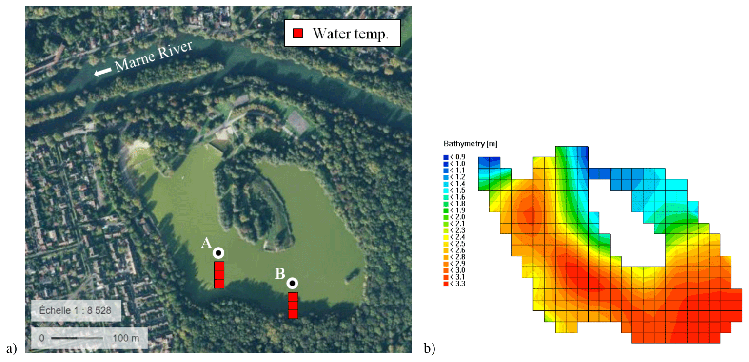
Figure 1 (a) Satellite picture of Lake Champs-sur-Marne (source: geoportail.fr) and sketch of the measuring system at the two locations (A and B). (b) Bathymetry and horizontal mesh of the study site as used in Delft3D.

The lake was formed in the 1940s by excavation and now represents a valuable and popular recreational area. However, it suffers from strong eutrophic conditions and experiences severe harmful algal blooms, especially between late spring and early autumn. In particular, cyanobacteria such as Microcystis and Aphanizomenon, capable of producing toxins, often proliferate and become the dominant species in the lake. This regularly leads to bathing bans and to access restrictions. For these reasons, the lake is subject to periodic monitoring. A high-frequency (every 10 min) in situ measuring system was installed at two different locations (A and B) during spring 2015. Each measuring site is equipped with sensors at three depths: below the surface at 0.5 m depth, in the middle of the water column at 1.5 m, and above the sediment at 2.5 m (Tran Khac et al., 2018). Water temperature is recorded at the surface and bottom layers with a precision of 0.02 ^∘C and a resolution of 0.05 ^∘C through the thermal sensor SP2T10 (nke INSTRUMENT^®), and through the MPx multi-parameter sensor (nke INSTRUMENT^®) at the middle of the water column with a precision and resolution of 0.05 ^∘C (see Fig. 1a). High-frequency water temperature observations are used here for the calibration and validation of the hydrodynamic model.

Lake Champs-sur-Marne is polymictic and its thermal behaviour is strongly influenced by meteorological conditions. Between March and November, periods of thermal stratification alternate with mixing and overturn of the water column. Depending on meteorological conditions, thermal stratification might form during the day and break up at night as well as last up to two or three consecutive weeks.

2.2 The model

2.2.1 Presentation of Delft3D-FLOW

The hydrodynamics of the study site were simulated with the FLOW module of the Delft3D modelling suite (Deltares, 2014). Delft3D-FLOW is a well known hydrodynamic model that has been applied in various contexts such as estuaries, rivers, lakes, and reservoirs (Piccolroaz et al., 2019; Chanudet et al., 2012; Soulignac et al., 2017). It solves the Reynolds-averaged Navier–Stokes equations for an incompressible fluid under the shallow water and the Boussinesq assumptions. The time integration of the partial differential equations is done through an alternate direction implicit method (Deltares, 2014; Leendertse, 1967). For the spatial discretization of the horizontal advection terms the cyclic scheme was selected (Stelling and Leendertse, 1992).

The bathymetry and the 2D mesh of the domain representing the study site are shown in Fig. 1b. The surface of the lake is divided into 255 20 m × 20 m cells. The Z model was implemented for the discretization of the vertical axes, with 12 fixed parallel horizontal layers of 30 cm thickness. It is generally accepted that horizontal layers help avoid artificial mixing, thus improving model results in terms of thermal stratification (Hodges, 2014). Turbulent eddy viscosity and diffusivity were computed through the k–ε turbulence closure model. Background values were set to zero [m² s⁻¹] for vertical viscosity and diffusivity, while they were set to 0.01 m² s⁻¹ for horizontal viscosity and diffusivity, after Soulignac et al. (2017) and according to the grid size. Bottom roughness was computed through Chézy's formulation with the default value for the Chézy coefficient of 65 m${}^{\mathrm{1}/\mathrm{2}}$ s⁻¹.

The computation of the heat exchange at the air–water interface is done through Murakami's model (Murakami et al., 1985). It requires, as input, the time series of relative humidity [–], air temperature [^∘C], net solar radiation [J s⁻¹ m⁻²], wind speed [m s⁻1], and wind direction [^∘ N] as well as constant values for sky cloudiness [–] and Secchi depth [m]. The heat flux model computes the heat budget at the air–water interface by taking into account the net incident solar radiation (Q_s), the heat losses due to back radiation (long wave, Q_b) and evaporation (latent heat flux, Q_e), and the sensible convective heat flux (Q_c). The total upward heat flux through the air–water interface (Q) is therefore

$$\begin{array}{}\text{(1)}& Q=-Q_{\mathrm{s}}+Q_{\mathrm{b}}+Q_{\mathrm{e}}+Q_{\mathrm{c}}.\end{array}$$

Finally, evaporative mass flux is here neglected and water volume and depth are therefore considered constants. These assumptions make it possible to exclusively analyse the impact of changes in the climatic forcing.

2.2.2 Meteorological input data

The meteorological forcing for this study comes from the spatialized SAFRAN (Système d'Analyse Fournissant des Renseignements Atmosphériques à la Neige) meteorological analysis system (Durand et al., 1993). SAFRAN is part of the SAFRAN-ISBA-MODCOU chain of reanalysis that covers the hydrological cycle over France, including meteorology, snow and ice formation, and hydrology (Habets et al., 2008). SAFRAN integrates spatialized data from meteorological models with various sources of observations through data assimilation techniques in order to create a consistent and spatially detailed record of meteorological data over the French territory. Its outcomes have been thoroughly validated against observed series (Quintana-Seguí et al., 2008) and tested as inputs to hydrological models (Raimonet et al., 2017). The data are spatialized on a regular square grid (8 km between each cell centre) that covers the entire French territory. The location of Lake Champs-sur-Marne falls midway on the axis connecting the centres of SAFRAN cells number 1457 (north of the lake) and 1566 (south of the lake). The average of these two cells was therefore considered representative of the conditions over the study site and used as input for the hydrodynamic model.

The data downloaded from the SAFRAN suite were temperature [^∘C], specific humidity [–], solar radiation (direct and diffused) [W m⁻¹], and wind speed [m s⁻¹]. All these variables are well reproduced by SAFRAN (Quintana-Seguí et al., 2008). Data were downloaded at an hourly time step, in order to accurately simulate the daily variability of the thermal profile and improve the model performance. This is crucial in shallow water bodies, where thermal stratification and mixing can alternate between day and night. Specific humidity (SH) data had to be converted into relative humidity (RH) to match the input dataset needed by Delft3D. This was done through the following formula:

$$\begin{array}{}\text{(2)}& \mathrm{RH}=\mathrm{100}\cdot {\displaystyle \frac{w}{w_{\mathrm{s}}}}\approx \mathrm{100}\cdot {\displaystyle \frac{\mathrm{SH}}{w_{\mathrm{s}}}},\end{array}$$

where w is the mixing ratio of water with dry air [kg kg⁻¹], the subscript “s” stands for saturation conditions, and SH is the specific humidity, numerically very close to the mixing ratio value. The saturation mixing ratio can be calculated as follows:

$$\begin{array}{}\text{(3)}& w_{\mathrm{s}}={\displaystyle \frac{R_{\mathrm{a}}}{R_{\mathrm{v}}}}\cdot {\displaystyle \frac{e_{\mathrm{s}}}{p_{\mathrm{atm}}-e_{\mathrm{s}}}},\end{array}$$

where the atmospheric pressure (p_atm) was considered to be constant and equal to the global average: p_atm=1013 hPa. The ratio between the air and vapour ideal gas constants (R_a and R_v, respectively) is equal to 0.622. The partial vapour pressure at saturation (e_s) is temperature dependent and can be estimated (in hPa) through the Magnus equation:

$$\begin{array}{}\text{(4)}& e_{\mathrm{s}}=\mathrm{6.1094}\cdot \exp \left({\displaystyle \frac{\mathrm{17.625}\cdot T}{T+\mathrm{243.04}}}\right),\end{array}$$

where T is air temperature [^∘C]. The numerical coefficients in Eq. (4) were issued from Alduchov and Eskridge (1997). Finally, in order to complete the set of meteorological input for Delft3D, daily wind direction data were downloaded from the closest available MétéoFrance station (ID: 78621001 located in Trappes, roughly 40 km west of the study site) through the INRAE CLIMATIK platform (https://intranet.inrae.fr/climatik/, last access: 5 March 2020, in French) managed by the AgroClim laboratory of Avignon, France.

2.2.3 Calibration and validation

Delft3D-FLOW stands on a robust mathematical and physical structure and only few parameters have to be calibrated. Here, only those directly involved in the heat-flux model and in the wind module were calibrated: the Secchi depth [m], the mean cloud cover [–], and the wind drag coefficient [–]. The Secchi depth (H_S) is the parameter that defines water transparency. It is correlated with the penetration of solar radiation in water through the light extinction coefficient ($\mathit{\gamma }=\mathrm{1.7}/H_{\mathrm{S}}$; Poole and Atkins, 1929) and therefore has a strong influence on the stratification of the water column. In order to get a first estimate for the sky cloudiness parameter, cloud cover data from the MétéoFrance station in Trappes (ID: 78621001) were averaged over the calibration period. The wind drag coefficient was calibrated in order to take into account the presence of tall trees surrounding the contour of the lake, locally reducing wind speed. The calibration was done through a trial and error procedure based on high-frequency water temperature data at the surface, middle and bottom layers (0.5, 1.5, and 2.5 m depth, respectively) during 2016. The model was then run for validation over the period during which both meteorological data and in situ observations were available, i.e. from 15 May 2015 to 31 December 2017.

Model results were compared to water temperature data at three depths (surface, middle, and bottom of the water column) and two different locations (A and B). The root mean square error (RMSE) was calculated to evaluate model performances. For this purpose, high-frequency data were first averaged every hour to match the model output time step and cleaned from the outliers that arise from periodic sensor maintenance. The latter were defined as sudden water temperature variations (>1 ^∘C) over the 10 min separating two successive measurements and consequently erased.

2.3 Indices for the characterization of the lake thermal regime

The thermal regime of the lake is assessed directly through the analysis of model results in terms of water temperature and through a series of indices that explore the phenology of stratification and highlight the relationship between temperature and cyanobacteria production, which is described below. All indices are computed both on an annual and on a seasonal basis according to the following definitions for the four seasons: (i) January–March (winter), (ii) April–June (spring), (iii) July–September (summer), and (iv) October–December (autumn).

2.3.1 Stratification indices

In order to thoroughly characterize the phenology of stratification in Lake Champs-sur-Marne, two indices for the stability of the water column were calculated: the Schmidt stability index and an index based on the temperature difference between surface and bottom layers. The Schmidt stability index is a parameter often used in limnological studies to estimate the resistance of a water body to mixing and therefore its stability. It has been extensively used in the scientific literature to describe the strength of stratification in lakes and, more recently, to analyse its evolution over time in relation to climate change (Vinçon-Leite et al., 2014; Niedrist et al., 2018; Kraemer et al., 2015; Livingstone, 2003) and algal blooms (Wagner and Adrian, 2009). The Schmidt stability index (S) represents the amount of work per unit area that would be required to mix the lake water column at one time instant. It was calculated here following Idso's formulation (Idso, 1973) in which the vertical axis z is considered positive downwards from the surface to the maximum lake depth z_M [m]:

$$\begin{array}{}\text{(5)}& S={\displaystyle \frac{g}{A_{\mathrm{0}}}}\underset{\mathrm{0}}{\overset{z_{\mathrm{M}}}{\int }}\left(z_{\mathrm{v}}-z\right)\left({\mathit{\rho }}_{\mathrm{i}}-{\mathit{\rho }}_{\mathrm{v}}\right)A\left(z\right)\mathrm{d}z\left[\mathrm{J}{\mathrm{m}}^{-\mathrm{2}}\right],\end{array}$$

where

$$\begin{array}{}\text{(6)}& z_{\mathrm{v}}={\displaystyle \frac{\mathrm{1}}{V}}\underset{\mathrm{0}}{\overset{z_{\mathrm{M}}}{\int }}zA\left(z\right)\mathrm{d}z\end{array}$$

is the depth of the centre of volume of the lake, ρ_v [kg m⁻³] is water density at the depth of the centre of volume z_v, ρ_i is the mean uniform density, g [m s⁻²] is the acceleration of gravity, V [m³] and A₀ [m²] are, respectively, the volume and the surface area of the lake, and A(z) is the surface of the horizontal section of the lake at depth z. Computed for each time step, the Schmidt stability can also be averaged over each year or season.

Water resistance to mixing as estimated by the Schmidt stability index is closely correlated to temperature stratification. However, universal thresholds for the onset and breakdown of stratification are difficult to define based on this index and cannot be found in the literature, especially for shallow polymictic lakes. In order to assess the succession of stratification events in a polymictic water body, the lake was considered to be stably stratified during a day if the minimum of ΔT is greater than 1 ^∘C (Kerimoglu and Rinke, 2013; Magee and Wu, 2017). This allows us to identify all stably stratified days (SSDs) and to compute their total number over a year (annual SSDs) or over a season (seasonal SSDs), as defined in Sect. 2.3.

2.3.2 Growth rate and growing degree days

Changes in the thermal regime might impact primary production. Here, we make use of two indices as proxies of the potential growth of phytoplankton species: the thermal growth rate (GR) and the growing degree days (GDDs). Under the assumption of nutrient and light availability, phytoplankton growth rate can be modelled, for different species, as a function of temperature (T) as in Bernard and Rémond (2012). $\forall T\in [T_{\min }$, T_max]:

$$\begin{array}{}\text{(7)}& {\displaystyle }\begin{array}{rl}& \mathrm{GR}\left(T\right)=k_{\mathrm{opt}}{\displaystyle \frac{\left(T-T_{\max }\right){\left(T-T_{\min }\right)}^{\mathrm{2}}}{\left(T_{\mathrm{opt}}-T_{\min }\right)}}\\ & \times {\displaystyle \frac{\mathrm{1}}{\left(T_{\mathrm{opt}}-T_{\min }\right)\left(T-T_{\mathrm{opt}}\right)-\left(T_{\mathrm{opt}}-T_{\max }\left(T_{\mathrm{opt}}+T_{\min }-\mathrm{2}T\right)\right)}};\end{array}\end{array}$$

where k_opt is the optimal growth rate, T_min the minimal temperature, T_opt the optimal temperature, and T_max the maximal temperature. The model parameters were calibrated by You et al. (2018) through experimental data to describe the response to water temperature of Microcystis aeruginosa, a species of cyanobacteria present in Lake Champs-sur-Marne and often dominant in freshwater bodies globally. The same values are used in this work:

$$\begin{array}{}\text{(8)}& {\displaystyle }\begin{array}{rl}& T_{\min }=\mathrm{0}{}^{\circ }\mathrm{C},T_{\mathrm{opt}}=\mathrm{27.5}{}^{\circ }\mathrm{C},T_{\max }=\mathrm{38.4}{}^{\circ }\mathrm{C},\\ & k_{\mathrm{opt}}=\mathrm{0.74}{\mathrm{d}}^{-\mathrm{1}}.\end{array}\end{array}$$

Microcystis aeruginosa is thought to be favoured by the warmer water temperatures induced by climate change. However, the curve obtained from Eqs. (7) and (8) (shown in Fig. 2), is more generally intended to be representative of the typical thermal response of cyanobacteria with high optimum temperature. Mean annual and seasonal (according to Sect. 2.3) growth rates are calculated through Eq. (7) using simulated surface water temperature and analysed over space and time.

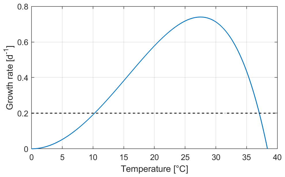
Figure 2 Thermal growth rate calculated after Eq. (7). The horizontal dashed line for GR = 0.2 d⁻¹ meets the curve at the temperature limits for the calculation of the GDDs (10 and 37 ^∘C, respectively).

The growing degree days are a weather-based indicator for biological growth, widely used in the field of agronomy. Based on air temperature, it gives an estimate of the rate of development and of the span of the growing season for terrestrial plants and insects. It is a useful indicator capable to link global warming and biology (Grigorieva et al., 2010; Schlenker et al., 2007). Approaches based on GDDs have been increasingly applied to phytoplankton communities and fisheries (e.g. Gillooly, 2000; Neuheimer and Taggart, 2007; Ralston et al., 2014; Dupuis and Hann, 2009) in order to correlate water temperature and phytoplankton growth while taking into account interannual variability. After Dupuis and Hann (2009), GDDs were calculated as follows:

$$\begin{array}{}\text{(9)}& {\displaystyle }\begin{array}{rl}\mathrm{GDD}\left(t\right)=& \sum _{i=t_{\mathrm{0}}}^t{a}_i\cdot \left(T_i-T_{\mathrm{base}}\right)\cdot \mathrm{\Delta }t,\\ & \mathrm{with}{a}_i=\left\{\begin{array}{cl}\mathrm{1}& \mathrm{if}{T}_{\mathrm{base}}<T_i<T_{\sup }\\ \mathrm{0}& \mathrm{elsewhere}\end{array}\right.,\end{array}\end{array}$$

where t is the time (here in days) and t₀ is the reference day to start the calculation, Δt is the time step (equal to 1 d), T_i is the daily average of the modelled surface water temperature of day i, and T_base (respectively, T_sup) is a physiological threshold below which (respectively, above which) growth does not occur. Compared to the formulation found in Dupuis and Hann (2009), an upper limit for growth was introduced here (T_sup) to take into account high-temperature stress. As for the GR, our focus here is on cyanobacteria. After Thomas et al. (2016) and based on the latitude of the study site, we set the base temperature at 10 ^∘C and the upper limit for growth at 37 ^∘C. For the calculation of the GDDs, this results in considering only temperatures that yield a GR above 0.2 d⁻¹ (see Fig. 2).

GDDs can be calculated on an annual or a seasonal basis by adjusting the values of t₀ and t. Annual GDDs are calculated from 1 January until 31 December. Seasonal GDDs are obtained according to the definitions in Sect. 2.3.

2.4 Long-term analysis

In the present paper we hindcast the long-term dynamics of a small, shallow urban lake between 1960 and 2017 in order to test the influence of climate change on such ecosystems.

2.4.1 Long-term trends

The long-term hydrodynamic simulation starts on 1 January 1960. No data were available to set the initial conditions of the model, neither in terms of water temperature, nor in terms of current velocities. However, the model is strongly driven by the meteorological data, and the influence of the initial condition vanishes after only a few days (Piccolroaz et al., 2019). Indeed, small perturbations in water temperature initial conditions (±2 ^∘C) were tested; these vanished in 5 to 7 d. The model was therefore initialized with water at rest and with a uniform water temperature of 7 ^∘C, the average of the water temperature recorded on the lake on 1 January in 2016–2019. Model results are stored at a hourly time step on every element of the mesh.

Model results at site A are analysed on an annual and seasonal basis for long-term trends in terms of water temperature (averaged over the water column) and through the indices defined in Sect. 2.3. The presence of long-term trends is tested (with a threshold for significance α=0.05) through the Mann–Kendall test (Mann, 1945; Kendall, 1975), a non-parametric test for the individuation of overall monotonic trends performed here through the MATLAB software (Burkey, 2020). The Mann–Kendall test is often preferred to simple linear regression in the analysis of meteorological and hydrological time series, as it does not require any assumptions on the distribution of the analysed dataset (Tímea et al., 2017; Wang et al., 2020). Once a trend is detected, its strength is evaluated through the Sen's slope estimator, which uses a linear model to evaluate the intensity of the trend (Sen, 1968).

Meteorological forcing is crucial for this work, as it drives the hydrodynamic model and represents the only source of variability in our modelling configuration. The presence of long-term trends in the meteorological dataset was also evaluated by applying the Mann–Kendall test and the Sen's slope estimator to their annual averages.

2.4.2 Spatial analysis

The long-term evolution and the spatial variability of the thermal regime of Lake Champs-sur-Marne was further analysed exploiting the 3D model simulations. Mean annual surface water temperature, annual SSDs, mean annual GR, and annual GDDs were computed on the whole computational domain, with the objective of investigating the relationship between climate change and time evolution of the spatial distribution of these variables. For each variable x, the overall mean annual value x_m (averaged over the complete domain) and the deviation from the mean value (x−x_m) were then computed. In order to quantify the spatial heterogeneity of these variables, the probability distribution of the deviation from the mean value of each variable was finally calculated on the computational domain and fitted, for each year, with a non-parametric Kernel probability distribution through the MATLAB pdf function. The resulting probability density function (PDF) was plotted over time as a heat map and the mean value as a simple line plot. This allows us to visualize both the time and the spatial evolution of the variable under consideration by looking at the mean value and at the range of values characterized by a non-zero probability.

During stably stratified periods, cyanobacteria are favoured over other algal groups because of their ability to move within the water column and possibly float towards the water surface (Humphries and Lyne, 1988; Wagner and Adrian, 2009; You et al., 2018). For this reason, the spatial analysis of the GRs and GDDs was completed by only calculating these two indices on stable stratified days during each year. The obtained GRs were further averaged for each cell over the local number of stably stratified days. Cells that showed an annual number of SSDs < 10 were discarded from this analysis. Finally, the resulting modified indices were analysed over space and time as described above by using a non-parametric Kernel probability distribution as an approximation of the PDF for each simulated year.

3 Results

3.1 Model calibration and validation

The model was calibrated on 2016 and validated on two other periods: from May to December 2015 and all of 2017. Field values for the Secchi depth in Lake Champs-sur-Marne vary between 0.5 and 3 m; using this range, the Secchi depth parameter was calibrated and finally set to 1.2 m. Sky cloudiness was calibrated and set to 80 % and a uniform wind drag coefficient was set to 0.005 [–].

Model performance during calibration and validation is shown in Fig. 3 relative to site A. Parity diagrams between observed and simulated water temperature are plotted for the surface, middle, and bottom layers (see panels a–c, respectively) and show an excellent agreement between observations and model results. A slight underestimation of surface water temperature can be noticed for the surface layer during the colder winter months as well as a slight overestimation of the highest values of water temperature by the model, especially for the middle and surface layers (see also Fig. 3d). However, the overall model performance is satisfactory for all three layers, with RMSE values between the simulated and observed water temperature of 0.85, 0.78, and 0.81 ^∘C at site A during calibration, respectively, for the surface (0.5 m), middle (1.5 m), and bottom (2.5 m) layers. Model results are also spatially robust and satisfactory for the validation periods, with similar RMSE values for sites A (surface: 1.0 ^∘C, middle: 0.96 ^∘C, and bottom: 0.96 ^∘C) and B (surface: 1.0 ^∘C, middle: 0.96 ^∘C, and bottom: 0.99 ^∘C).

Figure 3 Model performance during validation at site A. (a–c) Parity diagrams between simulations and observations for the surface, middle, and bottom layers, respectively. (d) Visual comparison of simulated and observed water temperature at the middle layer. (e) Modelled (orange) vs. observed (blue) temperature difference between the surface and bottom layer and relative comparison between the timing of observed and modelled stable stratification events (panels f and g, respectively).

Furthermore, the observed (blue) and simulated (orange) temperature difference between the surface and bottom layers is plotted in Fig. 3e, with a dashed lined representing the 1 ^∘C threshold for the definition of the SSD. Figure 3f and g shows the succession of stable stratification events as defined in Sect. 2.3.1 calculated through observations and model simulations, respectively. Some discrepancy is present, notably in spring 2016, which can be explained by a slight overestimation of surface temperature, combined with the threshold effect of the definition of the SSD. However, the model correctly captures the succession of stable stratification events both in terms of frequency and timing over the considered 3 year period.

Overall, the model results fit very well with the high-frequency water temperature data and accurately reproduce the water temperature dynamics, including the diurnal cycle and the stratification regime.

3.2 Long-term trend analysis

3.2.1 Meteorological input data

Annual averages of the SAFRAN dataset used as input in the Delft3D model were calculated from 1960 to 2017 and tested with the Mann–Kendall test. Strongly significant monotonic trends (p≪0.05) were found for the air temperature, solar radiation, and wind speed, as shown in Fig. 4. The Sen's slope estimator was used to test the intensity of the significant monotonic trends. Air temperature displays a considerable warming trend of 0.3 ^∘C per decade; solar radiation also shows a significant increasing trend, with an overall intensity of 3.5 W m⁻² per decade. Wind speed decreases quite sharply over time at an overall estimated rate of 0.2 m s⁻¹ per decade. While the increase in air temperature appears extremely linear (see Fig. 4a), a sharp shift in the behaviour of both solar radiation and wind speed appears around 1988 (Fig. 4b and c, respectively). A change-point detection was therefore performed on the latter two series and showed for both variables the existence of two significant sub-trends separated by a drastic shift towards the end of the 1980s. Both variables are characterized by a mild increase until 1987 (1988 for solar radiation) followed by a considerable decrease until the end of the available series. However, despite this piecewise linear behaviour, the presence of overall monotonic increasing (for solar radiation) or decreasing (for wind speed) trends is confirmed by the very low p values obtained for these variables through the Mann–Kendall test.

Figure 4 Annual averages of the three meteorological variables that exhibit significant monotonic trends: (a) air temperature, (b) solar radiation, and (c) wind speed. The relative overall trend intensity was evaluated through Sen's slope estimator for air temperature (orange dashed line, a), whereas a piecewise trend was calculated after change-point detection for solar radiation and wind speed (black dashed lines, b and c).

Finally, no significant trend was found for relative humidity and wind direction. These two variables appear to be stationary, with the former fluctuating around an annual average of roughly 80 % and the latter around an annual prevailing wind direction of 200^∘ N (southwest). Three of the five meteorological variables forcing the hydrodynamic model were therefore characterized by strongly significant monotonic trends over the past six decades, confirming changes in the climate of the region around the study site.

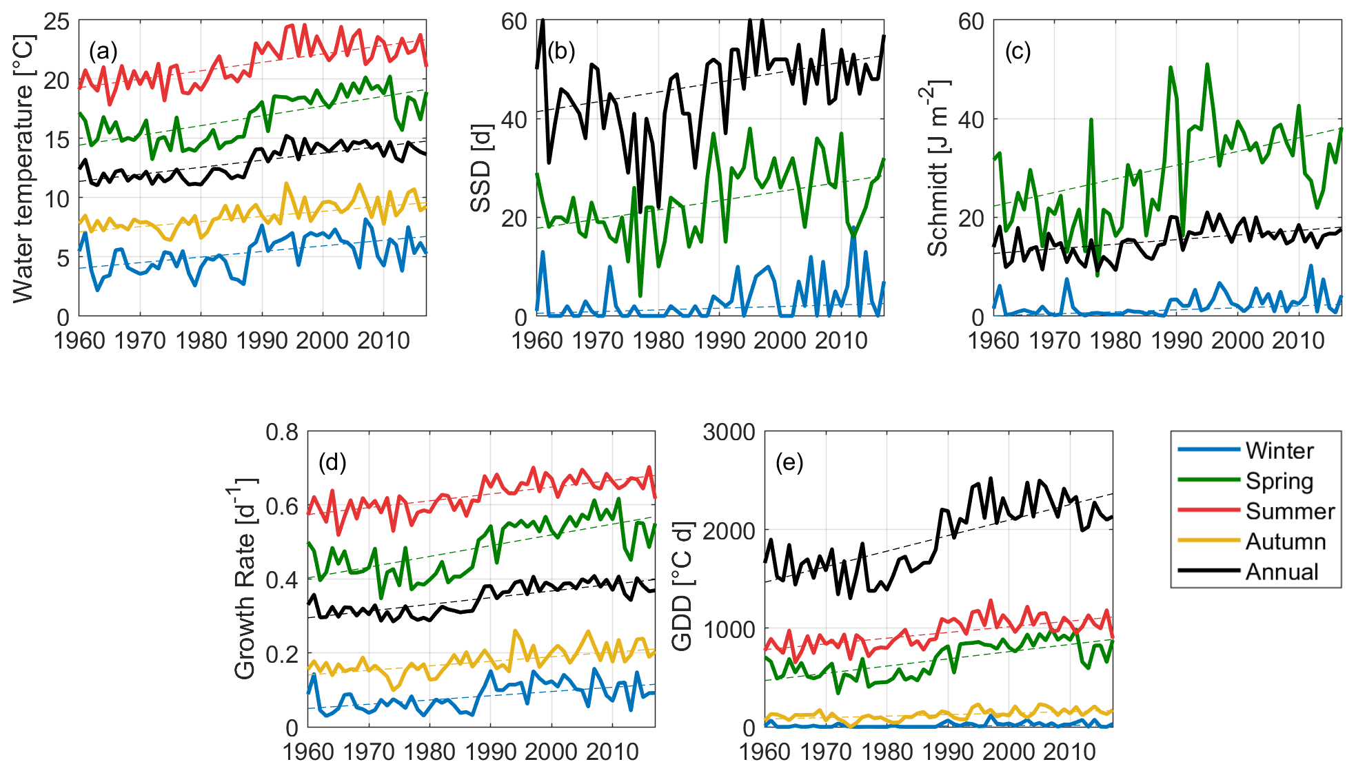
Figure 5 Statistically significant climate change trends at monitoring site A for the five indices, both on an annual (black) and seasonal (other colours) basis. (a) Water temperature (averaged on the water column); (b) number of stably stratified days (SSDs); (c) Schmidt stability; (d) Growth rate; and (e) growing degree days (GDDs). Blue lines represent the winter season, green lines represent spring, red lines are for summer trends, and yellow lines for autumn; black lines represent annual values.

3.2.2 Model results

Long-term monotonic trends were researched at site A on an annual and seasonal basis for: the mean water temperature (vertically averaged), number of stably stratified days (SSDs), mean Schmidt stability index, mean growth rate (GR), and growing degree days (GDDs). Figure 5 shows all the significant monotonic trends found from this analysis. On an annual basis, the Mann–Kendall test highlighted the presence of strongly significant increasing trends (p≪0.05) for all variables.

Mean annual water temperature shows a very sharp warming tendency of 0.6 ^∘C per decade (see Fig. 5a), even greater than what was found for air temperature (0.3 ^∘C per decade). The Pearson correlation coefficient (r) was calculated between water temperature and the five meteorological input variables in terms of annual averages in order to explain this behaviour. Modelled water temperature is strongly correlated with air temperature, solar radiation, and wind speed, with correlation coefficients of 0.8 for solar radiation and air temperature and −0.9 for wind speed. Water temperature shows a significant increase during all seasons, with higher slopes during spring and summer (0.8 and 0.7 ^∘C per decade, respectively), and a lower yet considerable intensity during autumn and winter (0.4 and 0.5 ^∘C per decade, respectively).

The warming trend is accompanied by reinforced stratification. An increase in water column stability is highlighted on an annual basis by both stratification indices: the annual number of SSDs increased on average of around two days per decade, while the Schmidt stability index increased by 0.9 J m⁻² per decade (Fig. 5b and c, respectively). Despite a warming trend being present in all seasons, both stratification-related indices only show significant increasing trends during winter (1 d per decade and 0.4 J m⁻² per decade) and spring (sharper trends of 1.8 d per decade and 2.6 J m⁻² per decade, for the seasonal SSDs and the Schmidt index, respectively). Furthermore, the number of stable stratification events (i.e. the count of the slots of consecutive SSDs during a year) was calculated to characterize the frequency of stable stratification. It did not show significant trends over time, varying between a minimum value of 8 to a maximum of 16 around an overall average of 12 stable stratification events. Similarly, the duration of the longest stable stratification event (i.e. the longest slot of consecutive SSDs in a year) did not show significant trends, but a high interannual variability. It varies around an average value of 11 d between a minimum value of 5 d and a maximum of 15 d.

The analysis of the growing degree days and of the mean growth rate shows the progressive improvement of conditions for cyanobacteria. The pattern of the mean annual GR is highly correlated to that of water temperature and shows a significant trend of 0.02 d⁻¹ per decade (black line in Fig. 5d). However, the stronger intensity of the trend for the GR during spring (0.03 d⁻¹ per decade) indicates an amplified effect of water temperature on the potential growth of cyanobacteria during this season. Annual GDDs (see Fig. 5e) show a considerable increasing rate of 157 d ^∘C per decade, with a strong shift around 1989. This behaviour cannot be regarded as linear and is highly influenced by the piecewise behaviour of mean annual solar radiation and wind speed. However, it corroborates the idea of a greater amount of thermal energy reaching the ecosystem at different rates but consistently throughout the four seasons.

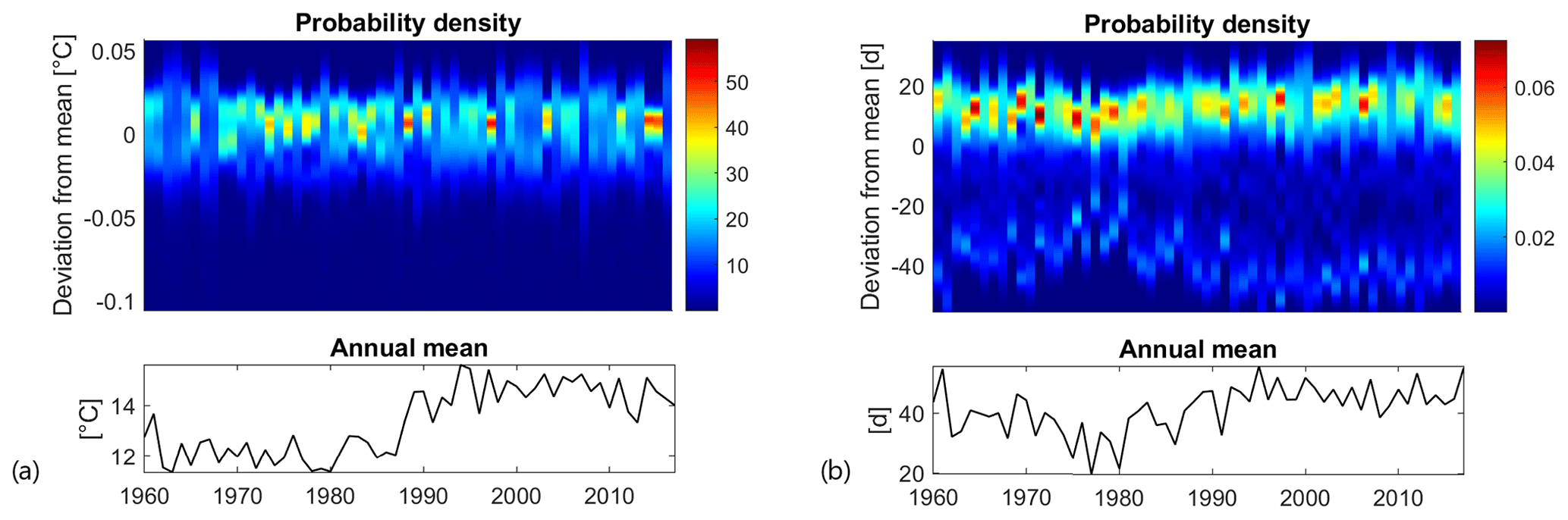
Figure 6 Top panels: time evolution of the probability density function of the anomalies (i.e. the spatial deviations of a variable to its annual mean over the lake). Bottom panels: time evolution of the annual mean calculated over the lake. (a) Mean annual surface water temperature; (b) annual SSDs.

The changes in the meteorological forcing clearly had an impact on the dynamics of the study site. The lake has sensibly warmed, its tendency to thermal stratification has increased, and the thermal conditions for cyanobacterial growth have improved. Spring shows the sharpest trends for all indices and might ultimately be the season suffering the strongest changes in terms of primary production and algal blooms.

3.3 Spatial analysis

Lakes are not spatially homogeneous systems. Heterogeneity can be generated by the interplay between bathymetric and morphological features or by particular meteorological conditions, especially in terms of wind direction.

In order to quantify the level of spatial variability in the lake, the deviations between local annual values (calculated for each computational cell) and their overall annual mean value (calculated on the complete domain) were calculated and fitted with a probability density function (PDF). As shown in Fig. 6a (top panel), mean annual surface water temperature is rather uniform over the study site. The difference between the maximum and minimum values is roughly 0.1 ^∘C (around 1 % of variability relative to the overall mean) and does not vary substantially over time. During the first half of the simulation period, and in particular between 1967 and 1987, the width of the PDFs (i.e. the domain on which PDFs are greater than 0) is narrower, reflecting a higher annual spatial uniformity than can be observed after 1990. After 1990, the width of the PDFs is indeed wider, with only a few exceptions where the PDFs are quite sharp. This change in the spatial distribution of annual surface water temperature before and after 1990 is accompanied by a sharp increase in the overall mean value (bottom panel in Fig. 6a), which is indeed greater (around 14.5 ^∘C) after 1990 than before (around 12 ^∘C).

The annual number of SSDs shows greater spatial heterogeneity (see Fig. 6b). The difference between the maximum and minimum SSD values varies between approximately 45 and 90 d. The spatial heterogeneity is mainly induced by bathymetry. Stable stratification only occurs in the deeper portion of the basin, while the northern part of the study site, namely the portion with a depth lower than 1.8 m (see Fig. 1b), remains constantly mixed according to our definition of SSDs. The PDF is dissymmetric, with the most probable value for the annual SSDs being higher than the overall annual mean by 10 to 15 d. As for the surface water temperature, the spatial heterogeneity of SSDs is higher after 1990 than before. In fact, a rather high correlation is present between the spatial distribution of the mean annual surface water temperature and SSDs. The correlation coefficient between the two variables in each simulated year varies between 0.4 and 0.8, with an overall mean of 0.62 and p values always lower than the threshold for significance (p=0.05). This suggests that surface water temperature tends to be slightly warmer in areas characterized by longer periods of stable stratification.

The thermal growth rate and the GDDs were analysed over the domain during stably stratified days, which are particularly favourable to the growth of cyanobacteria.

The thermal GR shows a low spatial heterogeneity that does not vary over time, as confirmed both by the PDF in Fig. 7a (top panel) and by the maps in Fig. 7b. The difference between the minimum and maximum GR values is around 0.03 d⁻¹ (around 5 % of the overall mean value), always rather centred around the overall mean. Calculated during stratification, the overall mean thermal GR takes high values (around 0.6 d⁻¹), comparable to those found at site A for the summer season (see the bottom panel of Figs. 7a and 5d).

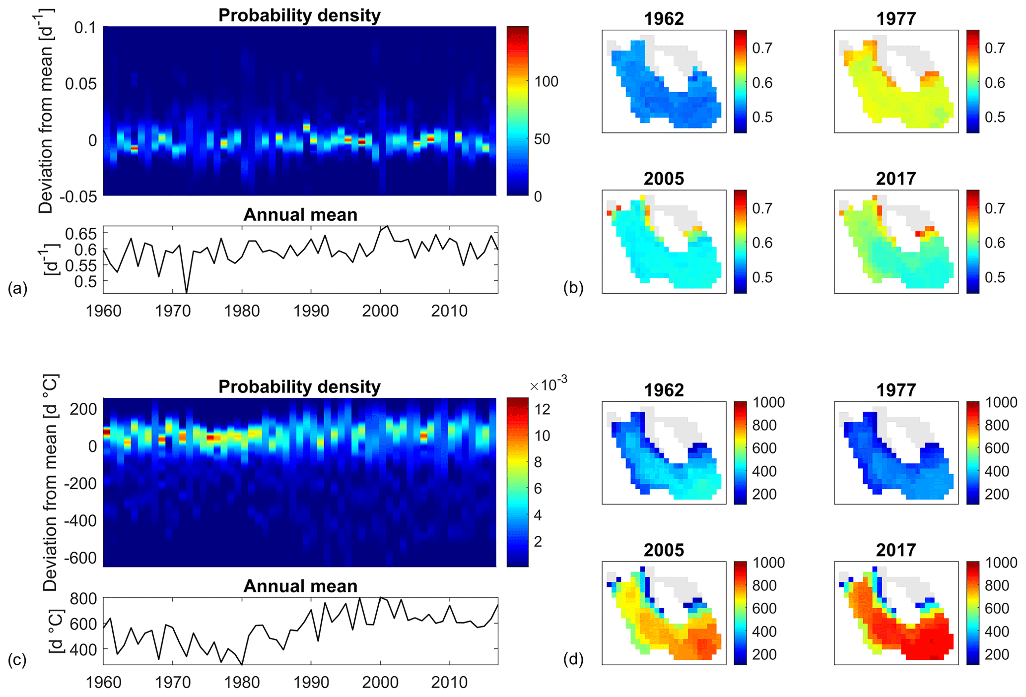
Figure 7 Spatial analysis of stratification. (a) Probability density function (PDF) for the mean GR during stratification over the computational domain and over time; (b) four examples of spatial distribution for the mean GR during stratification over the lake; (c) PDF for GDDs during stratification over the computational domain and over the years; (d) four examples of spatial distribution for annual GDDs during stratification over the lake. Grey cells in (b) and (d) do not stratify longer than 10 d over a year.

The overall mean annual GDDs increases over time (bottom panel of Fig. 7c) from around 400 d ^∘C before 1980 to 650 d ^∘C after. The PDF of the GDDs displays a clear increase in spatial heterogeneity (Fig. 7c). Its range increases substantially starting from the 1980s, roughly doubling from 100 d ^∘C before 1980 to around 200 d ^∘C afterwards. This is due to the concurring effects of warmer water temperature and higher number of stably stratified days in the calculation of the GDDs as defined in Sect. 2.3.2. In particular, part of the heterogeneity is induced by shallow areas of the water body that only account for a low number of SSDs and therefore for low values of GDD. The corresponding computational cells, not affected by stable stratification during the 1960s, are evermore likely to show stable stratification in the 2000s (see the maps in Fig. 7d). However, the maps for 2017 and 2005 also show a high heterogeneity in the deeper part of the water body.

4 Discussion

In the present paper, the thermal regime of a shallow urban lake was reconstituted over six decades (between 1960 and 2017) with a 3D thermal-hydrodynamic model. Simulation results were analysed over time (for long-term monotonic trends), and space (for spatial heterogeneity) through a series of indices that characterize the stratification and highlight the relationship between temperature and cyanobacteria production.

4.1 Meteorological forcing data

The model was forced with data from the SAFRAN meteorological reanalysis. Air temperature and solar radiation showed increasing monotonic trends (0.3 ^∘C per decade and 3.5 W m⁻² per decade, respectively), while wind speed showed a decreasing monotonic trend of −0.2 m s⁻¹ per decade. A shift was observed around 1987, especially in the data series of solar radiation and wind speed, and was confirmed by a change-point detection analysis. The existence of such shift in global climate during the 1980s has been highlighted by a number of studies using different data sources (Reid et al., 2016; Mariani et al., 2012; Gallagher et al., 2013).

Climate change in the Paris region has been assessed in the literature mainly in terms of air temperature (Perrier et al., 2005; Lemonsu et al., 2013). Compared to our result, a milder increasing trend of 0.1 ^∘C per decade was found based on ground measurements between 1900 to 1987, with a steeper increment of 0.7 ^∘C per decade appearing later on until 2005 (Perrier et al., 2005). Similarly, we also find a steeper trend of 0.55 ^∘C per decade during the years from 1987 to 2005. Less information can be found in the literature for solar radiation and wind speed. A decrease in wind speed on land has been found over Europe since 1980 (around −0.1 m s⁻¹ per decade) as part of a large-scale analysis of observations in the Northern Hemisphere (Vautard et al., 2010). On a global scale, an overall decreasing trend in wind speed was found over land in the period from 1985–2015 through meteorological reanalysis, principally over Europe, India, and western Africa (Torralba et al., 2017). In Southeast China, in the Lake Chaohu region, a strong decline in wind speed (China Meteorological station) was also found in the period from 1980–2016 (Zhang et al., 2020). An overall increase in surface solar radiation was recently found for Europe between 1983 and 2015, specifically 3 W m⁻² per decade for western Europe (Pfeifroth et al., 2018).

Meteorological reanalyses usually cover multi-decadal periods and have the great benefit of being spatialized over vast portions of the globe. Even though their use in limnological studies is quite recent, they have already been used to simulate water temperature (Layden et al., 2016; Piccolroaz et al., 2020), stratification dynamics (Frassl et al., 2018), and phytoplankton distribution (Soulignac et al., 2018). As shown in this work, their use as external forcing to thermal-hydrodynamic models can yield, provided that observations are available for calibration and validation, accurate simulations of the behaviour of water bodies even in the absence of local meteorological observations. This could open to a great range of applications in limnology and palaeolimnology (Jenny et al., 2016; Maier et al., 2019). The proposed methodology allows us to thoroughly reconstruct the behaviour of any water body both in time and space, independently of its proximity to meteorological stations. This is particularly interesting for small or remote water bodies that often lack long-term measurements.

4.2 Water temperature and stratification

Based on the 3D model results found for Lake Champs-sur-Marne, long-term trends were analysed in detail at site A. Significant increasing trends were detected for water temperature both on an annual and seasonal basis. The highest seasonal warming was found during spring and summer (0.8 and 0.7 ^∘C per decade, respectively). These trends are particularly intense and could have strong impacts on the ecosystem under examination. In particular, the intensity of these trends is greater than that suggested for summer water temperature in a large-scale analysis (0.53 ^∘C per decade) of lakes with similar changes in the meteorological forcing (O'Reilly et al., 2015). Furthermore, mean annual depth-averaged water temperature also increased at a considerable rate of 0.6 ^∘C per decade, greater than the rate found for air temperature, a behaviour also highlighted for other water bodies (Austin and Colman, 2007; Schneider et al., 2009). The piecewise linear behaviour of mean annual water temperature is induced by that of solar radiation and wind speed. In fact, similarly to what was found by Magee and Wu (2017), mean annual water temperature was highly correlated (i.e. $\left|r\right|>\mathrm{0.8}$) with air temperature, solar radiation, and wind speed. This suggests that meteorological variables have additive effects that enhance the response of the dependent variables. These effects might be particularly intense for wind over small, shallow lakes, due to their low volume-to-surface ratio.

Both stratification-related indices (SSDs and Schmidt stability) showed a significant mean annual increasing trend (3 d per decade and 1 J m⁻² per decade, respectively). Similar values were recently found for shallow water bodies in other long-term studies (Magee and Wu, 2017; Moras et al., 2019). However, despite a strong augmentation in water temperature, stratification did not show a significant increase during summer. In shallow polymictic lakes the water column is also mixed frequently during the warmer seasons. Summer surface and bottom water temperature increased at a very similar rate (0.7 ^∘C per decade) in the study site, resulting in small changes in Schmidt stability and number of SSDs. This result differs strongly from the behaviour of deeper monomictic or dimictic lakes, where the summer Schmidt stability often shows an increasing trend (e.g. Niedrist et al., 2018; Flaim et al., 2016) but it is not uncommon for shallow water bodies, where Schmidt stability can even show decreasing summer trends (Fu et al., 2020).

Stratification induces a separation between the sediment and the surface layers, influencing the distribution of nutrients and biomass over the water column. During stratification, due to the deoxygenation of the lake bottom layers, nutrients (phosphate in particular) are released from the sediment. In polymictic water bodies, when mixing occurs a replenishment of the whole water column with the nutrients released during previous stratification has been observed (Song et al., 2013; Wilhelm and Adrian, 2008). In Lake Champs-sur-Marne, neither the frequency nor the duration of the stable stratification events show a significant trend during the past decades. However, with a mean value of 12 annual separated stable stratification events lasting up to two consecutive weeks, the replenishment of the water column with nutrients is ensured. The multiple pulses associated with the alternation between mixing and stratification events are an important internal source of nutrients, especially in a lake such as the study site, whose water inflow is limited to underground waters.

The thermal regime was further characterized over the computational domain by analysing the spatial distribution of surface water temperature. While annual averages of surface water temperature are rather uniform over the domain, with around 0.1 ^∘C of difference between the maximal and minimal values, the bathymetric variations induced greater variability in the distribution of SSDs. The stratification regime drastically changes between the deeper portion of the water body and the shallower northern part. According to the definition of the SSD, stable stratification never occurs in cells with water depth lower than 1.8 m. In shallow water bodies, even small bathymetric variations can cause drastic differences in the thermal regime. Different regimes of mixing and stratification between shallower and deeper areas can result in considerable differences in the spatial distribution of nutrients, with effects on bloom initiation and phytoplankton growth, as well as on the resulting oxygen concentration. However, spatial heterogeneity of the mixing and stratification regime inside a water body is rarely addressed in the scientific literature, especially with regard to small, shallow lakes (e.g. Bachmann et al., 2000).

4.3 Indices for primary production

The thermal regime is a key factor in the regulation of the biogeochemical cycle and in the development of algal blooms. The worldwide intensification of harmful algal blooms over the past decades (Paerl and Huisman, 2008; Paerl and Paul, 2012; Wagner and Erickson, 2017) is often associated with climate change and nutrient enrichment (Zou et al., 2020; Huisman et al., 2018).

Due to their potential toxicity, cyanobacteria are of particular concern in freshwater management. Warmer water temperature can favour their growth because of their high optimal temperatures. However, they can proliferate under a wide range of temperatures (Lürling et al., 2013; Carey et al., 2012). The expression of the growth rate proposed by Bernard and Rémond (2012) (see Eq. 7) accounts for this dependence on water temperature. Based on this expression, the mean annual thermal growth rate of cyanobacteria showed a significant increasing monotonic trend of 0.02 d⁻¹ per decade. Compared to the initial annual value of roughly 0.3 d⁻¹ at the beginning of the 1960s, this results in a considerable total rate of change of +40 % at the end of the study period. Significant trends were also found during the four seasons, the highest being during spring (0.03 d⁻¹ per decade or +45 % of the initial value). The growing degree days (GDDs) of cyanobacteria were analysed here for a range of temperatures between 10 and 37 ^∘C, corresponding to thermal growth rates higher than 0.2 d⁻¹. However, given the temperate climate of the region under examination, the upper limit for growth did not have any effect on the results, while it could be an important parameter for species with lower optimum temperatures such as diatoms.

Whereas the growth rate gives an estimation of the mean value of cyanobacteria growth that can be computed on a seasonal and an annual basis, the GDD is a cumulative index that gives a measure of the amount of time and degrees available during a year for photosynthetic growth. Originating from the field of agronomy and forestry, it represents a “thermal time” and is considered a better descriptor of vegetal phenology than the simple Julian days (McMaster and Wilhelm, 1997). Under an appropriate temperature range, the GDD can be considered as representative for organism developmental time (Dupuis and Hann, 2009). The highest trend for GDDs was found on an annual basis (157 d ^∘C per decade), denoting that the temperatures favourable to cyanobacteria growth are more and more frequently reached. Seasonal trends varied greatly in intensity. The highest was found for spring (73 d ^∘C per decade) and represents, relative to the values in the early 1960s, a substantial increase of 90 % during the six decades under consideration. The trends found for winter and autumn are mild but denote an increased tendency to overpass the base temperature during these two seasons and therefore a dilatation of the season favourable to cyanobacteria growth.

Harmful algal blooms and phytoplankton dynamics depend on factors such as the settling or buoyancy rate of phytoplankton, the availability of nutrients over the water column, which can be enhanced by the release from the sediment, and the resuspension of particulate organic matter. In polymictic water bodies, the processes of sedimentation and resuspension are strongly influenced by the alternation between mixing and stratification (Song et al., 2013). Because of their ability to migrate within the water column, stratified environments are favourable to cyanobacteria (e.g. Carey et al., 2012; Aparicio Medrano et al., 2016). The co-occurrence of an increase of water temperature and of stable stratification could lead to an enhanced augmentation of cyanobacteria blooms. However, stratified conditions do not occur uniformly. Calculation of the thermal GR and GDDs quantifies the potential effect of water temperature on cyanobacteria growth under the hypothesis of nutrient and light availability. Their calculation during stratification allows us to address the combined effect of water temperature during a particularly favourable environmental conditions.

During stratification, the cyanobacteria GR was characterized by high values (around 0.6 d⁻¹) with a variability quite uniform over time of ±5 % over the study site. These values are comparable or even higher (until the 1990s) than those obtained during the summer season. The GDDs provide deeper insight into the interplay between temperature and stratification. The strong augmentation in the overall mean value of the GDDs during stratification confirms a concurring positive effect of the increase of water temperature and of the duration of stable stratification on the growth of cyanobacteria. Moreover, the greater spatial variability of GDD values during the second half of the simulation indicates that some parts of the lake will be more affected than others by the variation of water temperature and stratification. In particular, we observe the development over time of certain areas in the study site, especially the deeper part, with very high values of GDD under stratified conditions and that are therefore particularly favourable to cyanobacteria dominance and bloom initiation.

The combination of increasing trends for water temperature, stable stratification, and the widening of the growing season can favour the occurrence of harmful cyanobacterial blooms (Winder and Sommer, 2012; Jones and Brett, 2014; Noble and Hassall, 2015). If these trends are confirmed, cyanobacteria could become the dominant species in the study site in the future, seriously affecting the lake ecological network and its biodiversity (Rasconi et al., 2017; Toporowska and Pawlik-Skowronska, 2014).

4.4 Model-based approach

Through our modelling approach it was possible to reconstruct the thermal dynamics of a small, shallow lake and to thoroughly analyse its evolution over time and space. The use of an extensive dataset of high-frequency observations allowed us to test the model not only against the general seasonal water temperature pattern, but also against daily and sub-daily dynamics of stratification and mixing at two locations. Other works have focused on the hindcast of lakes thermal regime, successfully reconstructing their dynamics in order to analyse their evolution over time (e.g. Magee and Wu, 2017; Moras et al., 2019; Zhang et al., 2020; Stetler et al., 2020). Most of these studies, however, make use of a 1D approach. By means of a 3D model it is possible to aggregate information on both time and space (horizontal and vertical) through the use of appropriate indices. Our work demonstrates that even on a small water body spatial variations can be important and that their influence on the thermal and biological regime must be considered. It provides additional evidence that supports the hypothesis of a positive effect of climate change over cyanobacteria blooms.

Hydro- and thermal dynamics are at the core of the biogeochemical cycles, influencing transport, sediment resuspension, organic matter mineralization, and primary production. In this work, we focus on water temperature, quantifying its impact for stratification and primary production. The proposed methodology allows us to focus solely on the role of meteorological forcing, addressing its direct impact on the thermal regime and on primary production. However, other factors could have an even stronger impact: nutrient and light limitation or grazing could offset temperature-derived advantages (Elliott et al., 2006). These factors are not taken into account in this work, since it is focused on the impact of climate change from a thermal standpoint with all other factors being equal. This work opens up a wide range of possible additional analysis and further research. In particular, coupling with a biogeochemical model could give further insight into the impact of climate change on the ecological state of a water body. Such a study, however, would introduce additional sources of uncertainties, especially regarding the evolution of nutrient sources over time, and would only be useful if performed after a thorough analysis of the hydrodynamic and thermal regime.

5 Conclusions

In this work, the long-term thermal regime of a shallow urban lake is reconstructed through model simulations from 1960 to 2017. A series of indices are proposed with the objective of thoroughly describing the thermal regime of shallow water bodies in relation to stratification dynamics and cyanobacterial production. The meteorological dataset is derived from the SAFRAN reanalysis and shows a significant increase in air temperature and solar radiation and a significant decrease in wind speed, with a regime shift in the late 1980s. Simulation results show that small urban lakes react rapidly and strongly to external meteorological conditions, with only limited resilience to climatic shifts. The additive effect of increasing solar radiation and air temperature and decreasing wind speed acts on different terms of the heat budget at the lake surface, enhancing the changes found in the lake. The mean water warming of 0.6 ^∘C per decade represents an increase of 32 % in water temperature values between 1960 and 2017 and is much stronger than the air warming (0.3 ^∘C per decade, i.e. an increase of 18 % during the same period). The impact on stratification and cyanobacteria production is even more alarming, with an increase of over 30 % of the stability indices and over 60 % of the growing degree days during the past six decades. Spring shows the sharpest trends in terms of water temperature, water column stability (Schmidt and SSDs), and growing degree days, and might ultimately be the season suffering the strongest changes in terms of primary production and algal blooms. The spatial heterogeneity found for thermal stratification and growing degree days might also concur to locally create conditions particularly favourable for cyanobacteria blooms. These tendencies could favour early phytoplankton blooms (during late winter or spring) and contribute to the proliferation of cyanobacteria and ultimately to the degradation of the whole aquatic ecosystem. Our results highlight the importance of a 3D approach to thoroughly infer the dynamics of a water body. Horizontal patterns can be particularly strong for shallow lakes due to the relative importance of bathymetric variations.

Small, shallow lakes are extremely widespread ecosystems. Our results suggest that such systems experience considerable thermal stress caused by climate change and that, in nutrient-enriched systems, cyanobacteria dominance could become a widespread issue in the future decades.