Large ensemble climate model simulations: introduction, overview, and future prospects for utilising multiple types of large ensemble

Single model initial-condition large ensembles (SMILEs) are valuable tools that can be used to investigate the climate system. SMILEs allow scientists to quantify and separate the internal variability of the climate system and its response to external forcing, with different types of SMILEs appropriate to answer different scientific questions. In this editorial we first provide an introduction to SMILEs and an overview of the studies in the special issue “Large Ensemble Climate Model Simulations: Exploring Natural Variability, Change Signals and Impacts”. These studies analyse a range of different types of SMILEs including global climate models (GCMs), regionally downscaled climate models (RCMs), a hydrological model with input from a RCM SMILE, a SMILE with prescribed sea surface temperature (SST) built for event attribution, a SMILE that assimilates observed data, and an initialised regional model. These studies provide novel methods, that can be used with SMILEs. The methods published in this issue include a snapshot empirical orthogonal function analysis used to investigate El Niño–Southern Oscillation teleconnections; the partitioning of future uncertainty into model differences, internal variability, and scenario choices; a weighting scheme for multi-model ensembles that can incorporate SMILEs; and a method to identify the required ensemble size for any given problem. Studies in this special issue also focus on RCM SMILEs, with projections of the North Atlantic Oscillation and its regional impacts assessed over Europe, and an RCM SMILE intercomparison. Finally a subset of studies investigate projected impacts of global warming, with increased water flows projected for future hydrometeorological events in southern Ontario; precipitation projections over central Europe are investigated and found to be inconsistent across models in the Alps, with a continuation of past tendencies in Mid-Europe; and equatorial Asia is found to have an increase in the probability of large fire and drought events under higher levels of warming. These studies demonstrate the utility of different types of SMILEs. In the second part of this editorial we provide a perspective on how three types of SMILEs could be combined to exploit the advantages of each. To do so we use a GCM SMILE and an RCM SMILE with all forcings, as well as a naturally forced GCM SMILE (nat-GCM) over the European domain. We utilise one of the key advantages of SMILEs, precisely separating the forced response and internal variability within an individual model to investigate a variety of simple questions. Broadly we show that the GCM can be used to investigate broad-scale patterns and can be directly compared to the nat-GCM to attribute forced changes to either anthropogenic emissions or volcanoes. The RCM provides high-resolution spatial information of both the forced change and the internal variability around this change at different warming levels. By combining all three ensembles we can gain information that would not be available using a single type of SMILE alone, providing a perspective on future research that could be undertaken using these tools.

1 An introduction to SMILEs

A single model initial-condition large ensemble (SMILE; see Table 1 for a glossary of abbreviations) is a set of model simulations starting from different initial conditions but produced with a single climate model and identical external forcing. Over the last decade SMILEs have been increasingly utilised in climate science (e.g. Zelle et al., 2005; Branstator and Selten, 2009; Kay et al., 2015; Frankignoul et al., 2017; Kirchmeier-Young et al., 2017; Sanderson et al., 2018; Stolpe et al., 2018; Maher et al., 2019; Deser et al., 2020). The value of SMILEs comes from the ability to quantify and separate the internal variability of the climate system and the forced response to changes in external forcing (e.g. Kay et al., 2015; Maher et al., 2019). Additional value comes from identifying and robustly sampling extreme events (e.g. heatwaves, floods, and droughts), which potentially have large impacts on people despite their low probability of occurrence (e.g. Fischer et al., 2013; Suarez-Gutierrez et al., 2018; Haugen et al., 2018). Here, SMILEs allow a more accurate sampling of the entire probability distribution, including the tails of the distribution where extreme events occur. This sampling additionally allows for future projections of events with long return periods to be made (e.g. van der Wiel et al., 2019). Different applications require different types of SMILEs. For example, to investigate questions that involve the entire climate system, global climate model (GCM) SMILEs must be used. However, to investigate impacts at local scales, regionally downscaled climate model (RCM) SMILEs are more appropriate. Here, we provide an overview of the exciting new science published in the special issue “Large Ensemble Climate Model Simulations: Exploring Natural Variability, Change Signals and Impacts”. We also present a perspective on the value of combining different types of existing SMILEs, by presenting four simple examples combining a GCM, RCM, and a natural forcing only GCM SMILE.

(Kushner et al., 2018; Kirchmeier-Young et al., 2017)(Kay et al., 2015)(Leduc et al., 2019)(Martynov et al., 2013)(Ehmele et al., 2020)(Watanabe et al., 2010)(Maher et al., 2019)

Table 1 Glossary of acronyms presented in alphabetical order for three categories: large ensemble types, Earth system acronyms, and specific climate models and modelling projects.

A large body of literature already exists using individual GCM SMILEs. The majority of studies have used the Community Earth System Model Large Ensemble (CESM-LE; Kay et al., 2015) as it has been available for the longest period of time (since 2015). Many studies have utilised the power of SMILEs to investigate the internal variability of the climate system (e.g. Fasullo and Nerem, 2016; Frankignoul et al., 2017; Smith and Jahn, 2019; Dai and Bloecker, 2019) and extreme events (e.g. Diffenbaugh et al., 2015; Gibson et al., 2017; Kirchmeier-Young et al., 2017; Tebaldi and Wehner, 2018; Wang et al., 2018). Studies have also looked into all components of the climate system, including the biosphere, with oceanic biogeochemistry included in these models (e.g. Rodgers et al., 2015; McKinley et al., 2016; Lovenduski et al., 2016; Krumhardt et al., 2017; Li and Ilyina, 2018; Schlunegger et al., 2019). More recently studies have utilised a combination of multiple SMILEs (e.g. Maher et al., 2018; Fasullo et al., 2020; Schlunegger et al., 2020; Zhou et al., 2020), allowing the assessment of model agreement between the SMILEs for individual scientific questions. SMILEs from seven GCMs have now become publicly available (Deser et al., 2020). In the reference paper for this model archive, Deser et al. (2020) have demonstrated that this collection “offers an unprecedented opportunity for evaluating and comparing models’ forced responses and their internal variability”. Despite their recent availability these SMILEs are already widely used. Some examples include the investigation of the role of internal variability and model differences in affecting future projections (Maher et al., 2020; Lehner et al., 2020; Maher et al., 2021), trends in sea surface temperature patterns (Olonscheck et al., 2020) and South American summer rainfall (Díaz et al., 2021), the decadal modulation of global warming (Liguori et al., 2020), the time of emergence of ocean biogeochemical trends (Schlunegger et al., 2020), and Arctic extremes (Landrum and Holland, 2020). These SMILEs have also been investigated for use in adaption decision making (Mankin et al., 2020), hydroclimate uncertainty in east–central Europe (Topál et al., 2020), and uncertainty in projections of global land monsoon precipitation (Zhou et al., 2020).

GCM SMILEs have been used not just to investigate scientific questions, they have also been utilised as test beds for new approaches, and tools to inform policy makers. They have been used to create an observational large ensemble (McKinnon et al., 2017; McKinnon and Deser, 2018) and test dynamical adjustment techniques (Deser et al., 2016; Lehner et al., 2017). They have also been used to develop new methodologies such as utilising the ensemble dimension for analysis (Herein et al., 2017; Maher et al., 2018, 2019; Haszpra et al., 2020a, b) and to develop and test statistical methods for isolating the forced response (Sippel et al., 2020; Wills et al., 2020). Such ensembles have additionally provided important information for policy makers, such as whether emission reductions are likely to be detectable in the coming years, or whether they could be masked by internal variability (Lehner et al., 2016; Tebaldi and Wehner, 2018; Marotzke, 2019; Spring and Ilyina, 2020).

Targeted experiments that utilise the main advantage of SMILEs, i.e. to isolate the forced response and internal variability, have also been run that both build on and complement the GCM studies. Some examples of such targeted experiments include single-forcing SMILE experiments, which have been used for detection and attribution (e.g. Kirchmeier-Young et al., 2017), and RCM SMILEs, which are increasingly being used for impact studies (e.g. Leduc et al., 2016). Other complementary experiments include a large ensemble which is designed to test the sensitivity of the historical simulations to known uncertainties in aerosol forcing (Dittus et al., 2020). Atmosphere- or ocean-only large ensembles are also used to quantify the internal variability in select parts of the climate system when the rest of the climate system is fixed to observed values (Gates, 1992; Barnett et al., 1997; Penduff et al., 2014). In the following paragraphs we outline the utility of some of these targeted experiments, focusing on single-forcing and RCM ensembles as these are able to explore a wide range of possible past and future states as they include all components of the climate system.

Single-forcing SMILEs are used to separate the role of different forcings and to attribute change to different drivers. The first single-forcing SMILE was run as part of the Canadian large ensemble experiments (Kirchmeier-Young et al., 2017). This ensemble consists of a GCM run for 50 members with all forcings, 50 members with only anthropogenic aerosols, and 50 members with only natural (volcanic and solar) forcing. These experiments were completed for the period 1950–2020. The Canadian large ensemble has been used to show that extreme fire events in Canada are 1.5 to 6 times more likely under anthropogenic greenhouse gas forcing compared to a climate with natural forcing alone (Kirchmeier-Young et al., 2017). This ensemble has been used to show that anthropogenic aerosols offset the effects of anthropogenic greenhouse gases on ice cover in the mid-twentieth century (Gagné et al., 2017a) and that large volcanic eruptions result in an increase in Arctic sea ice following the eruption (Gagné et al., 2017b). This single-forcing SMILE has also been used in combination with another SMILE (CESM-LE) to investigate the detection timescale of tropospheric warming in single-ensemble members (Santer et al., 2019). Here, the authors provided an estimate as to how uncertainty due to internal variability can affect the time required to detect patterns of change and how dependent this detection time is on different types of forcing from the single-forcing simulations.

A different type of single-forcing SMILE has also been run where an individual forcing is set to a specific value but all others remain as in the full experiment as opposed to fixing all but one forcing as in the Canadian large ensemble (Pendergrass et al., 2019). By keeping aerosols fixed at the pre-industrial level Pendergrass et al. (2019) are able to identify the relationship between global warming and extreme precipitation. Previous studies have assumed that single-forcing experiments can be linearly added to recreate an all-forcing experiment result. Pendergrass et al. (2019) find that the relationship in their model is quadratic and stress that the response of extreme precipitation to aerosols is state dependent and as such the linearity assumption that is often used in the context of single-forcing experiments does not hold for this quantity. These results demonstrate the need for many different types of experiment to answer different questions and show that when there is large internal variability these experiments must be run as large ensembles.

RCMs allow for higher-resolution studies and smaller-scale impact-based studies than GCMs. Internal variability is found to be larger at smaller spatio-temporal scales (Aalbers et al., 2018) demonstrating the need for RCM SMILEs that can resolve these scales and provide a large sample size (Wood and Ludwig, 2020). RCMs have the advantage the they can better represent local values. For example Leduc et al. (2019) found a better representation of extreme temperature and precipitation locally in an RCM SMILE compared to its driving GCM SMILE. In applying machine learning techniques, RCM SMILEs were of great service to detect frequencies, intensities, and the temporal dynamics of Vb cyclones (a specific type of cyclone associated with extreme precipitation and flooding over Europe) and the associated patterns of extreme precipitation over central Europe (Mittermeier et al., 2019). Multiple RCM SMILEs are now becoming available (e.g. Aalbers et al., 2018; Leduc et al., 2019; Kirchmeier-Young et al., 2019; Lang and Mikolajewicz, 2020), which are currently run over European and North American domains. Having multiple RCM SMILEs is important as different RCMs have different magnitudes of internal variability. This was demonstrated by von Trentini et al. (2019), who found that internal variability of a single RCM SMILE covers some but not all of the spread in a multi-model RCM ensemble.

Large ensembles of RCMs are currently used for a variety of purposes. They can be used for event attribution at higher-resolution scales than GCMs (e.g. Kirchmeier-Young et al., 2019). They can also be used to look at local changes in internal variability (e.g. Leduc et al., 2019) and projected changes in the signal-to-noise ratio of both the mean and importantly extremes (Aalbers et al., 2018; Poschlod et al., 2020b). With the availability of SMILEs, impact studies, e.g. in hydrology, can assess new ways of analysing the impacts of climate change on hydrological processes, reaching from water balance studies and flow regime changes (Poschlod et al., 2020a) to extreme events, such as floods (Willkofer and Ludwig, 2020). In order to deal with the challenges of dynamically altered extreme events under climate change, often compound events, SMILEs can introduce the concept of analysing the relevance of climate variability by means of spatially explicit and process-based models, assessing the non-linear response to multiple meteorological drivers, such as in alpine snow cover dynamics (Willibald et al., 2020) and (managed) land surface responses (Zscheischler et al., 2018). SMILEs can be used as new instruments to provide the data density and the parameter space to deal with the high process complexity and (often) data scarcity, especially when operational flood forecasting or flood risk management is targeted (Willkofer and Ludwig, 2020). For all of these cases, SMILEs can serve as a provider of coherent and standardised data, providing a very useful extension to the existing top–down modelling chain concepts, by enabling the application of artificial intelligence, machine learning, and big data concepts for impact studies.

Given the recent availability of many of the aforementioned tools, SMILEs are currently only beginning to be utilised to their full power. There are unexploited opportunities for a wide range of disciplines, such as hydrology, biogeosciences, and climate dynamics. The special issue “Large Ensemble Climate Model Simulations: Exploring Natural Variability, Change Signals and Impacts” was open to submissions which exploited these new opportunities and explored how a combined analysis of the different types of existing large ensembles can advance our knowledge in different fields. Submissions were particularly invited to use new methods to investigate these topics. The new contributions published in this special issue will be summarised in the following section.

2 Advances in knowledge from this special issue

The nine studies published in “Large Ensemble Climate Model Simulations: Exploring Natural Variability, Change Signals and Impacts” have utilised a wide range of types of SMILEs including seven GCM SMILEs, three RCM SMILEs, hydrological models driven by RCMs, a SMILE for event attribution (prescribed sea surface temperature), a data-assimilated SMILE, and an initialised regional SMILE. As such the studies published in this special issue cover a wide range of SMILEs that can be used for a variety of purposes. The studies fall into the following categories: (1) novel methods, (2) RCM large ensemble evaluation and use, and (3) impacts of global warming. They will be presented in the following sections.

Novel methods

Four novel methodologies have been published in this special issue. The study of Haszpra et al. (2020a) entitled “Investigating ENSO and its teleconnections under climate change in an ensemble view – a new perspective”, uses a single GCM SMILE (CESM-LE) and the snapshot empirical orthogonal function (SEOF) analysis method to investigate the El Niño–Southern Oscillation (ENSO) pattern and amplitude changes in each individual season by applying an SEOF across the ensemble for each month of the year. Haszpra et al. (2020a) are then able to investigate teleconnections of ENSO (taken as the first principal component) with precipitation data by computing lagged regressions between the two variables. The use of this methodology has allowed Haszpra et al. (2020a) to identify an increase in the sea surface temperature (SST) fluctuations in the ENSO region that is most pronounced in June, July, August, and September but also occurs in December, January, and February. They have also used this methodology to identify which ENSO teleconnections are projected to change and to become more pronounced in this SMILE. For example they find enhanced positive precipitation correlations with ENSO in central Africa and on the western coast of South America and a more pronounced anticorrelation over Australia and the southern edge of South America that occur in June, July, August, and September.

Hawkins and Sutton (2009) originally proposed a methodology to partition uncertainty into that from model differences, internal variability, and scenario choices using a multi-model ensemble. Lehner et al. (2020) revisit this methodology in a study entitled “Partitioning climate projection uncertainty with multiple large ensembles and CMIP5/6”. Here, using seven GCM SMILEs and the Coupled Model Intercomparison Projects 5 and 6 (CMIP5 & 6), they show that the original approach works well at global and regional scales; however, for local scales a more accurate partitioning of uncertainty is needed, which can only be achieved using the SMILEs. They additionally demonstrate that differences between CMIP5 and 6 can to some extent be reconciled by normalising projections by global mean temperature or applying a simple model weighting that targets high climate sensitivities. This shows that the differences between CMIP5 and 6 results are largely due to the high climate sensitivities found in some of the CMIP6 models.

With the newly available CMIP6 data, where some models have one ensemble member and some models have many, the question of how to combine these data in the most meaningful way has been asked. Merrifield et al. (2020) use three GCM SMILEs and 88 members of CMIP5 to provide a comprehensive evaluation of five different weighting strategies for a multi-model ensemble that includes some SMILEs in “An investigation of weighting schemes suitable for incorporating large ensembles into multi-model ensembles”. They provide a comprehensive explanation of how one would determine weights for any application and demonstrate that reasonable weights can be generated when taking both model performance and independence into account. Having such a methodology that allows the use of all available information is highly valuable and will be applicable as the new CMIP6 data becomes available. Due to its importance for upcoming analyses of the CMIP6 simulations this article was published in ESD's highlight section.

With the recent availability of many SMILEs, which vary in size from as few as 15 members to as many as 200 members, it is now important to ask the following question: “How large does a large ensemble need to be?”. Milinski et al. (2020) do this, presenting a method to estimate the required ensemble size for any given problem using a single GCM SMILE (Max Planck Institute Grand Ensemble; MPI-GE) and a long pre-industrial control simulation to test the method. They demonstrate that the required ensemble size depends on both the question asked and the acceptable error to the user. In general the signal (response to external forcing) and the magnitude of the internal variability determine how large the ensemble needs to be. The smallest ensemble size is needed for estimating the forced response, with a larger size needed to quantify internal variability and the highest ensemble size required to detect changes in internal variability. They also demonstrate that more members are needed for regional than global quantities. This method can be used by any scientist to identify the ensemble size required before starting their study.

These novel methodologies demonstrate the utility of SMILEs as a test bed and show that when using SMILEs traditional methods can be redefined and new methods developed, which exploit the power of large ensembles.

RCM large ensemble evaluation and use

RCM SMILEs have been used extensively in this special issue with two studies specifically evaluating how well RCMs perform. Böhnisch et al. (2020) use the 50-member Canadian Regional Climate Model Large Ensemble (CRCM5-LE) to investigate the regional response to the North Atlantic Oscillation (NAO). In particular, they investigate how well the NAO signal propagates from the GCM domain to the RCM domain in a study entitled “Using a nested single model large ensemble to assess the internal variability of the North Atlantic Oscillation and its climatic implications for Central Europe”. They find that both models reproduce the NAO pattern, with the large-scale NAO propagating properly into the finer-scale RCM domain; however, the RCM produces more realistic spatial climate patterns, likely due to the additional topographic features. These features in the RCM are also found to provide value in evaluating regional NAO impacts, with the relationship between the NAO and climate over Europe predicted to slightly weaken in the future. This study highlights how dynamically downscaling a GCM SMILE can help to understand regional impacts of major modes of internal variability by combining the advantages of a large sample size with high resolution to represent regional processes.

A multi-RCM SMILE comparison over Europe was provided by von Trentini et al. (2020). They compare three RCM SMILEs with observations in “Comparing interannual variability in three regional single model initial-condition large ensembles (SMILEs) over Europe”. This study evaluates seasonal temperature, precipitation, dry periods, and heatwaves. They find that the three ensembles agree well with observations for interannual variability and that despite some model differences, the sign of projected future variability changes is similar across models. Specifically, they find an increase in summer temperature and precipitation variability as well as decreases in winter temperature and precipitation variability under strong global warming. They also find increased variability in summer in the number of heatwaves and the maximum length of a dry period in two of the three models. The study highlights the differences in projected interannual variability between ensemble members and shows that SMILEs are necessary to robustly quantify the significance of such changes.

These two studies – Böhnisch et al. (2020) and von Trentini et al. (2020) – have both demonstrated the value of using an RCM SMILE in addition to a GCM SMILE (Böhnisch et al., 2020) and provided some confidence in projections across the European domain (von Trentini et al., 2020).

Impacts of global warming

Many studies in this special issue address the changing probabilities of extreme events and their impacts under a changing climate. SMILEs are the perfect tool to investigate such events because they sample the probability distribution at each time step and allow assessment of changes in the probabilities of events such as floods, droughts, and heatwaves. In this special issue Canadian winter hydrometeorological extreme events are investigated by Champagne et al. (2020), European flooding events are investigated by Ehmele et al. (2020), and fire and drought in Asia are investigated by Shiogama et al. (2020).

Champagne et al. (2020) published “Winter hydrometeorological extreme events modulated by large-scale atmospheric circulation in southern Ontario”. In this study they use a single RCM SMILE (CRCM5-LE) to create a new winter compound index to investigate the contribution of the combination of rain and snowmelt to extreme events. They then use the output from the RCM SMILE as input to a hydrological model to identify the necessary conditions needed for high flows to occur in three southern Ontario watersheds and to project their future evolution. They find that the RCM output is realistic when compared to observational data and project an increase in the future number of heavy rain and warm events associated with high flows particularly in the vicinity of Lake Erie, especially when there are high 500mb geopotential height anomalies centred on the eastern Great Lakes and the Atlantic Ocean. Using the RCM SMILE they are able to investigate how the internal variability of climate will modulate the future evolution of these hydrometeorological extremes and show that the increase in events can be amplified or attenuated depending on the location of pressure systems modulated by internal variability.

Ehmele et al. (2020) use a single RCM SMILE (Large Ensemble of Regional Climate Model Simulations for Europe; LAERTES-EU) that consists of both long-term and initialised simulations as well as runs that assimilate reanalysis data to look at “Long-term variance of heavy precipitation across central Europe using a large ensemble of regional climate model simulations”. They find that the model represents observed extreme precipitation well. When considering future projections, the upcoming decade shows a continuation of past tendencies in Mid-Europe, with increasing heavy precipitation, with no clear signal for the Alps. Additionally they use the power of the large ensemble to show that there are phases of increased and decreased heavy precipitation that are due to internal variability alone. Generally, they emphasise the benefit of RCM SMILEs for an improved estimation of extreme values, building on robust statistics.

A large event attribution ensemble (Model for Interdisciplinary Research on Climate 5; MIROC5), where sea surface temperatures and ice are prescribed, is used to demonstrate the role of historical anthropogenic warming on droughts and fires in equatorial Asia (Shiogama et al., 2020). In the study entitled “Historical and future anthropogenic warming effects on droughts, fires and fire emissions of CO₂ and PM_2.5 in equatorial Asia when 2015-like El Niño events occur”, Shiogama et al. (2020) show significant increases in burned area, carbon dioxide, and PM_2.5 emissions at 1.5 and 2 ^∘C of warming, with the chance of exceeding the large 2015 event reaching 100 % under 3 ^∘C of warming. They also argue for including fires in future climate modelling scenarios as these can affect global carbon dioxide emissions.

Finally the previously discussed papers of Böhnisch et al. (2020) and Haszpra et al. (2020a) also investigate impacts of the modes of variability: NAO and ENSO respectively. Böhnisch et al. (2020) find an increasing the frequency of a negative NAO that favours colder and harsher winters in Europe. Haszpra et al. (2020a) demonstrate that some ENSO teleconnections can change, with some increasing in strength while others decrease, which will have different impacts in different regions. An example of the changes they find is an increase in precipitation teleconnections between ENSO and Australia and Africa in their respective winters at the end of the century.

Overall these studies on changing events and their impacts are made possible by the use of SMILEs, where extreme events are well sampled and changes in modes of variability can be separated from large internal variability. These studies are relevant for policy and planning, with Ehmele et al. (2020) demonstrating high variability in precipitation over different decades in Europe, Champagne et al. (2020) showing changes in flood risk in Ontario in their study, and Shiogama et al. (2020) finding an increase in the risk of large fires and their impacts in equatorial Asia under increasing warming.

3 Perspectives on new tools and their value

There are now many SMILEs available for use in the climate community. These include GCM SMILEs, atmosphere- and ocean-only SMILEs, single forced SMILEs, SMILEs forced with all except one forcing, RCM SMILEs, and SMILE experiments with different sets of forcing such as varying aerosols. In this section we present some simple examples to investigate the value of combining different types of SMILEs and demonstrate how future research can benefit from using the SMILEs which are already available. To do this we use the Canadian Earth System Model Large Ensemble (CanESM2; Kirchmeier-Young et al., 2017; Kushner et al., 2018) because it has 50 members of both the full forced ensemble (1950–2100; historical and RCP8.5) and 50 members of natural-only forcing (solar and volcanic forcing; 1950–2020). These SMILEs are henceforth referred to as GCM and nat-GCM. We combine the GCM and nat-GCM with the Canadian Regional Climate Model Large Ensemble (CRCM5-LE as part of the ClimEx project; Leduc et al., 2019), which uses the Canadian Regional Climate Model (12km resolution CRCM5; Martynov et al., 2013; Šeparović et al., 2013) with the CanESM2 GCM SMILE with all forcings used as boundary conditions. We utilise the European domain from this SMILE. This SMILE will be referred to as RCM for the rest of this study.

To investigate the value of combining the GCM and RCM SMILEs we will evaluate changes in both near-surface air temperature (SAT) and precipitation at multiple warming levels. The warming levels are 1 K (2002), 1.5 K (2015), 2 K (2028), 3 K (2048), and 4 K (2067). The years at which each warming level occurs are found using the ensemble mean from the GCM as compared to the pre-industrial control. We use an 11-year window centred on each warming level to analyse the data. Projected changes are always shown relative to the 1 K level (similar to the present day; Allen et al., 2018) and are computed individually for each ensemble member. This choice allows us to investigate future changes above the present day. This is particularly relevant in light of the targets of 1.5 and 2 K set by the Paris Agreement. In addition to SAT and precipitation we use the variable maximum daily temperature (tasmax in the ensemble output), henceforth referred to as max-SAT. For the GCM this variable is output as the monthly mean of the daily maximum temperature. We average the daily data from the RCM to be comparable. For the analyses presented in this editorial summer is computed as the average of June, July, and August (JJA) and winter as the average of December, January, and February (DJF).

The ensemble mean SAT and precipitation at 1 K of warming are shown for the GCM and RCM SMILEs in Fig. 1. The continental outlines highlight the resolution difference between the GCM and the RCM. The patterns of both SAT and precipitation are broadly similar between the GCM and the RCM, with warmer temperatures to the south and more precipitation to the north-west of the domain, particularly over the United Kingdom and western Norway. Figure 1 also shows that the increased resolution of the RCM allows the local patterns to be better resolved and highlights the effects of features such as coastlines and mountains. Subtracting the GCM from the RCM shows that the RCM tends to be slightly cooler and wetter than the GCM. While there has been no comprehensive validation of whether the GCM or RCM is more realistic, when compared to observations over Europe, Leduc et al. (2019) found a better representation of extreme precipitation and local extremes in the RCM than the GCM, particularly over coastal and mountain regions, due to the higher resolution. In general due to their higher-resolution RCMs provide a more realistic representation of smaller scales, such as land–sea contrasts and orography and, at higher resolutions, lakes and rivers (e.g. Lucas-Picher et al., 2017; Rummukainen, 2010; Christensen and Kjellström, 2020; Feser et al., 2011). This makes RCMs more suited for looking at impacts at local scales and more reliable than GCMs when looking at small regions and events on shorter timescales (Rummukainen, 2016).

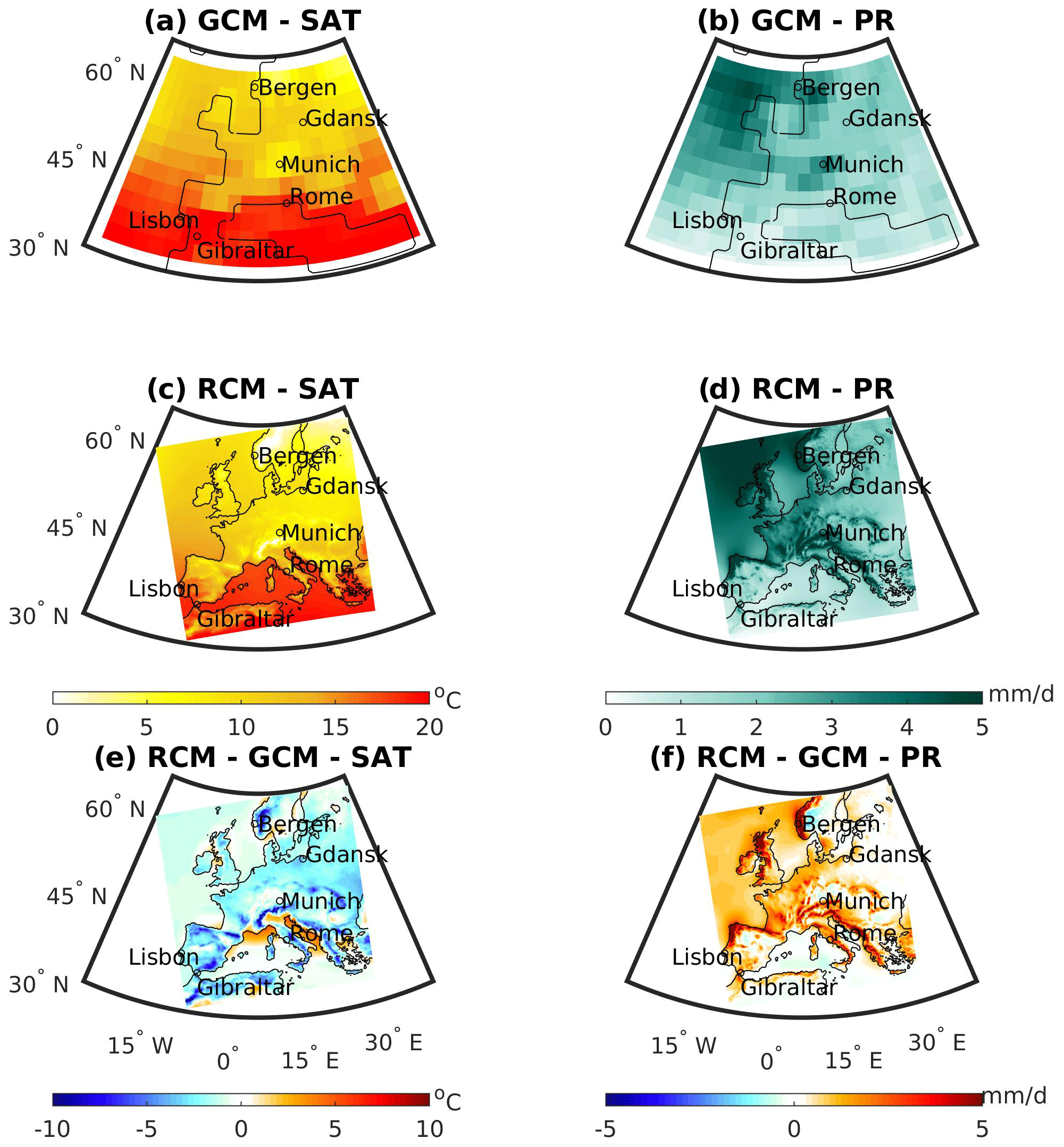
Figure 1 Ensemble mean surface air temperature (SAT) and precipitation in the GCM (a, b) and RCM (c, d) SMILEs over Europe at 1 K warming (2002). The difference between the RCM and GCM SMILEs is shown in (e) and (f). We use an 11-year window around the warming year to analyse the data. The cities investigated in Figs. 3 and 4 are shown on the maps. Continental borders are plotted for each model's native grid.

To demonstrate the utility of combining different types of SMILE we consider the following simple examples:

1. We ask whether the SAT and precipitation responses over Europe are linear with global warming in both the GCM and RCM.

2. We investigate SAT, max-SAT, and precipitation projections in a subset of European cities in both the GCM and RCM at 1.5, 2, 3, and 4 K global warming. These cities are shown in Fig. 1 and are chosen due to their location near the coastline or in mountainous regions, where the increased resolution of the RCM may provide additional information.

3. We investigate whether there are forced changes and, if so, their drivers in summer SAT variability at 1.5 and 4 K, by combining the GCM, nat-GCM, and RCM

4. Finally we investigate the European seasonal response to large volcanic eruptions using all three SMILEs.

Regional response to global warming

In this section we ask whether the European SAT and precipitation responses are linear with global warming. By using the GCM SMILE we can pinpoint specifically when the model has reached a given level of global warming. By computing the ensemble mean at each warming level, we can precisely identify the forced response at each warming level in both the GCM and RCM. Due to the large ensemble sizes, differences between the GCM and RCM can be directly attributed to differences in the forced response between the two SMILEs. Using an RCM for climate projections has previously been shown to both provide additional value, but to also introduce additional biases (Jacob et al., 2020). The added value has been shown to come from better representation of physical mechanisms as well as the better representation of underlying topography (Dudhia, 2014; Mearns et al., 2013; Di Luca et al., 2013; Evans and McCabe, 2013), suggesting the RCM projections may be regionally more reliable than the GCM.

We find that the scaled SAT and precipitation patterns at 1.5 K are very similar in the GCM and RCM (Fig. 2a, c, e, g). These patterns also resemble those found in the Coordinated Downscaling Experiment in the European Domain (EURO-CORDEX) experiment (Jacob et al., 2018). By looking at the scaled 4 K response as compared to the scaled 1.5 K response (Fig. 2b, f), we find that the SAT response is slightly non-linear with south-western Europe warming more at 4 K and northern and eastern Europe warming less relative to the scaled 1.5 K response. The RCM and GCM agree well on this non-linearity. When considering precipitation, the response is again non-linear (Fig. 2d, h), with the increase in precipitation over northern Europe not as large at 4 K as at 1.5 K, but the decrease over southern Europe larger. While there is agreement between the GCM and RCM on the broad-scale pattern, the RCM is needed to resolve the local precipitation non-linearity and the response over southern Europe. The result that there is more added value of the RCM for precipitation than SAT is in agreement with previous work as precipitation is more affected by orography and small-scale processes than SAT (Lucas-Picher et al., 2017; Christensen and Kjellström, 2020; Feser et al., 2011; Rummukainen, 2016).

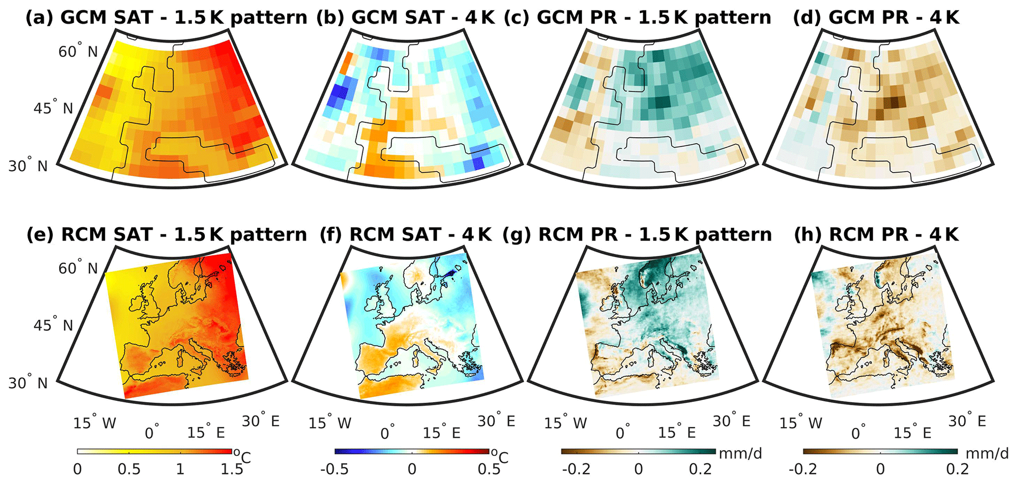
Figure 2 Surface air temperature (SAT) and precipitation change over Europe scaled by the globally averaged SAT change. (a) Scaled SAT change at 1.5 K in the GCM, (b) scaled SAT change at 4 K with scaled SAT change at 1.5 K subtracted in the GCM, (c) scaled precipitation change at 1.5 K in the GCM, (d) scaled precipitation change at 4 K with scaled SAT change at 1.5 K precipitation in the GCM, (e) Scaled SAT change at 1.5 K in the RCM, (f) scaled SAT change at 4 K with scaled SAT change at 1.5 K subtracted in the RCM, (g) scaled precipitation change at 1.5 K in the RCM, and (h) scaled precipitation change at 4 K with scaled SAT change at 1.5 K precipitation in the RCM. Changes are computed relative to the pattern at 1 K of global warming. Continental borders are shown for the each model's native grid. The scaled changes in panels (a) and (d) are computed as the pointwise SAT at 1.5 K minus the pointwise SAT at 1 K dived by the global mean warming above 1 K (i.e. 0.5 K) in each individual ensemble member. The patterns in (b) and (f) use the same calculation at 4 K, with the patterns from (a) and (e) subtracted from them. The ensemble mean is taken prior to the subtraction. The same process is computed in the right-hand panels for precipitation.

Projections in individual European cities

Given that the RCM provides the most additional information at local scales, particularly near the coastlines and orography, we next investigate some major cities across Europe (shown in Fig. 1), all of which are near the coastline or orography. Here, we investigate how the warming in an individual city compares to the global mean warming by utilising the power of the SMILEs and computing the forced response in each city. For example if we take a city such as Rome, we can ask the question of whether we expect Rome to warm more or less than the global mean. We can then ask whether this relative warming is linear with global warming; i.e. if at 2 K warming Rome warms more than the global mean, does it warm the same amount more at 4 K? Finally because we are using SMILEs we can look at the range of warming in Rome that we could observe due to internal variability. For example if the mean warming is the same as the global mean warming, how much more or less warming than the mean could we observe due to internal variability? Here, we will assess if the answers to these questions differ between the GCM and RCM.

We find a range of results across the three cities (Fig. 3). When we consider the ensemble mean warming, Lisbon warms less than the global mean, while Rome warms slightly more and Gdańsk warms similarly. Rome and Gdańsk warm more in summer and in the summer maximum temperature than the global mean, especially at larger levels of warming. This means that someone living in these cities would likely experience more warming than the global mean level would suggest. Surprisingly, we find that the RCM shows less non-linearity in the relative warming than the GCM. This gives slightly lower projected temperatures and a slightly more promising outlook when using the RCM as compared to the GCM.

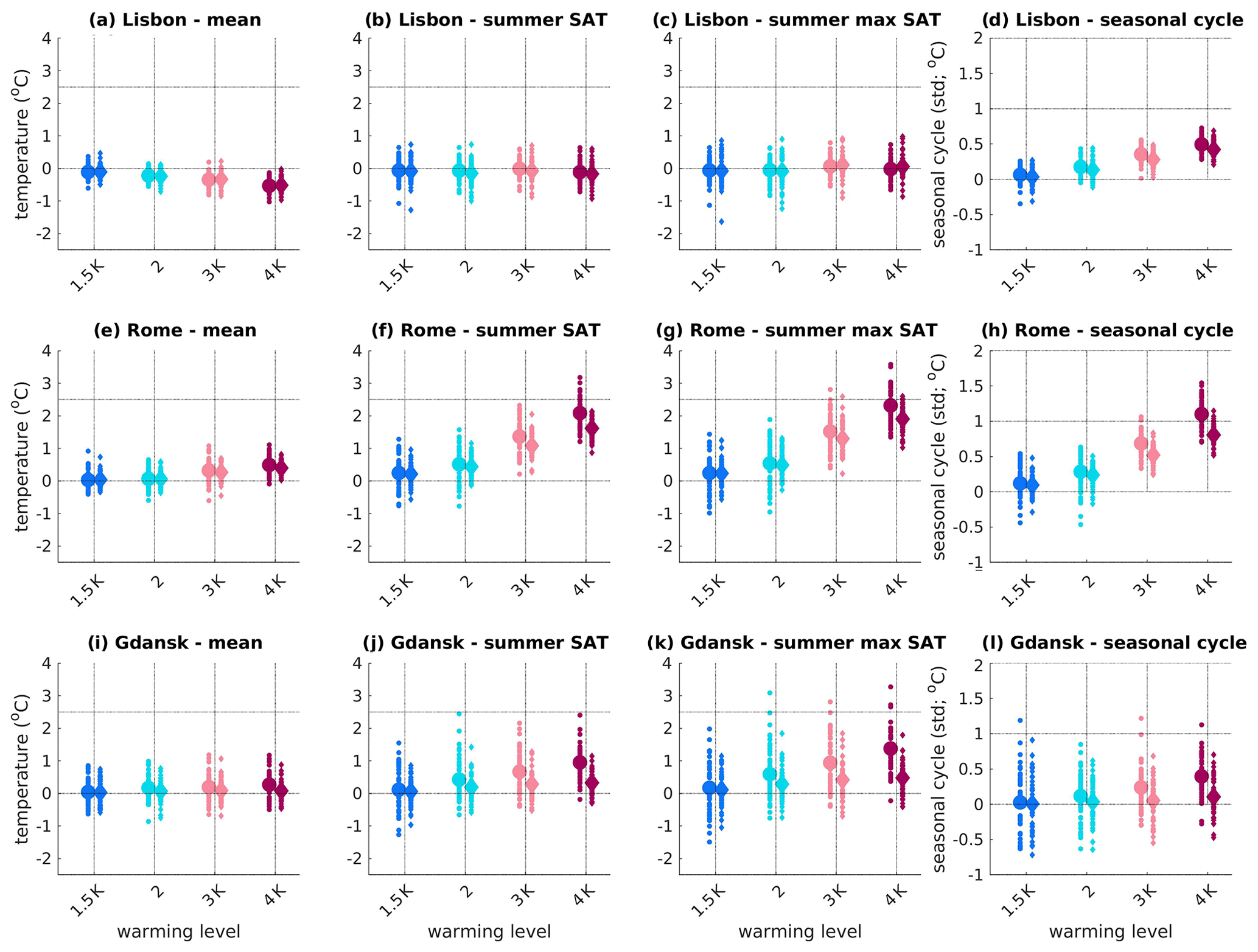
Figure 3 Annual-mean surface air temperature (SAT) (a, e, i), summer SAT (b, f, j), and summer max-SAT (c, g, k) and the seasonal cycle change (d, h, l) shown at each warming level relative to 1 K of global warming. Shown for the GCM (circles) and the RCM (diamonds). Each ensemble member is shown in the small symbols with the ensemble mean in the large symbol. Shown for (a–d) Lisbon (38.7223^∘ N, 9.1393^∘ W), (e–h) Rome (41.9028^∘ N,12.4964^∘ E), and (i–l) Gdańsk (54.3520^∘ N, 18.6466^∘ E). Each ensemble members change is computed relative to itself at 1 K, with the global warming above 1 K then subtracted for all variables except the seasonal cycle. The seasonal cycle is computed as the standard deviation over all 12 months after the 11-year period has been averaged.

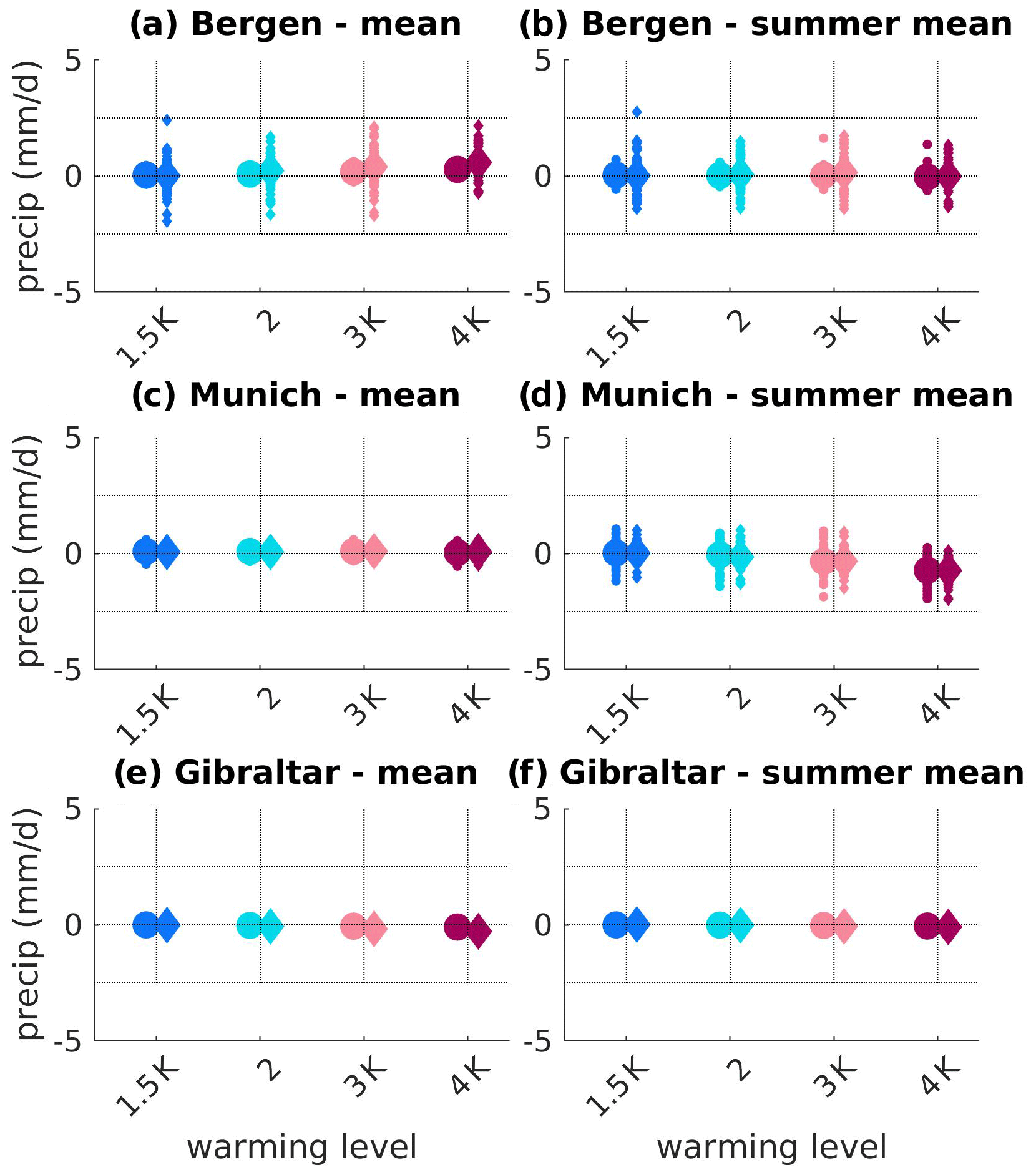
Figure 4 Annual-mean precipitation (a, c, e) and summer precipitation (b, d, f) shown at each warming level relative to 1 K of global warming. Shown for the GCM (circles) and the RCM (diamonds). Each ensemble member is shown in the small symbols with the ensemble mean in the large symbol. Shown for (a–b) Bergen (60.3913^∘ N, 5.3221^∘ E), (c–d) Munich (48.1351^∘ N, 11.5820^∘ E), and (e–f) Gibraltar (36.1408^∘ N, 5.3536^∘ W). Each ensemble members change is computed relative to itself at 1 K.

We next consider the seasonal cycle. Here, an increase means that summer warms more than winter. The seasonal cycle increases in Lisbon and Rome. This change and the internal variability of the change are slightly smaller in the RCM than the GCM, suggesting that the local range of possible observed changes could be smaller than expected from the GCM. Where the internal variability no longer crosses the zero line (e.g. 3–4 K warming for Rome and Lisbon), we expect to see an increase in the seasonal cycle in all members, although the magnitude of the change depends on how the system evolves in each individual member. This is an important advantage of using SMILEs as we can assess the range of possible futures that could be observed due to the combination of increasing greenhouse gases and internal variability.

Finally we investigate how precipitation is projected to change in a city on the coastline with high mean precipitation (Bergen, Fig. 4a, b), a city on the coastline with low mean precipitation (Gibraltar, Fig. 4e, f), and a city surrounded by high orography (Munich, Fig. 4c, d). We find limited changes in the forced response for both mean and summer precipitation in all three cities as compared to the precipitation at 1 K of warming. There is little difference in the mean changes between the GCM and RCM. However, the RCM can have very different internal variability than the GCM. We find larger variability in the RCM over Bergen. This means that while there is little mean change in Bergen, at any warming level the city could observe a 2.5 mm/d decrease or 3 mm/d increase in both the mean and summer mean precipitation in any given year due to internal variability alone. This demonstrates the additional value of an RCM SMILE in planning for potential observed changes in local locations.

Insights into forced changes in temperature variability

Using SMILEs we are now able to quantify changes in internal variability at different warming levels. This was not previously possible with single runs of climate models. By pooling the summer data for all ensemble members for the 11-year window around each warming level we can calculate the internal variability at each grid point in the European domain for each individual warming level. To do this we take a standard deviation across the pooled data. Figure 5 shows the GCM summer SAT internal variability at 1.5 K and the difference between the GCM and the RCM and the nat-GCM. We find that the GCM has slightly less variability over north-western Europe as compared to the nat-GCM, suggesting that summer variability at 1.5 K is decreased over this region as compared to natural unforced variability alone. The RCM generally has less variability than the GCM, which indicates that the GCM might overestimate summer SAT variability over Europe. We then consider the change in variability at 4 K as compared to 1.5 K in both the GCM and RCM. We find a projected increase in variability over all of the European land mass, except Portugal and Spain, that is larger in the RCM than the GCM. This tells us that local processes in the RCM result in a larger increase in summer temperature variability, although the overall increase in both the RCM and GCM displays the same pattern.

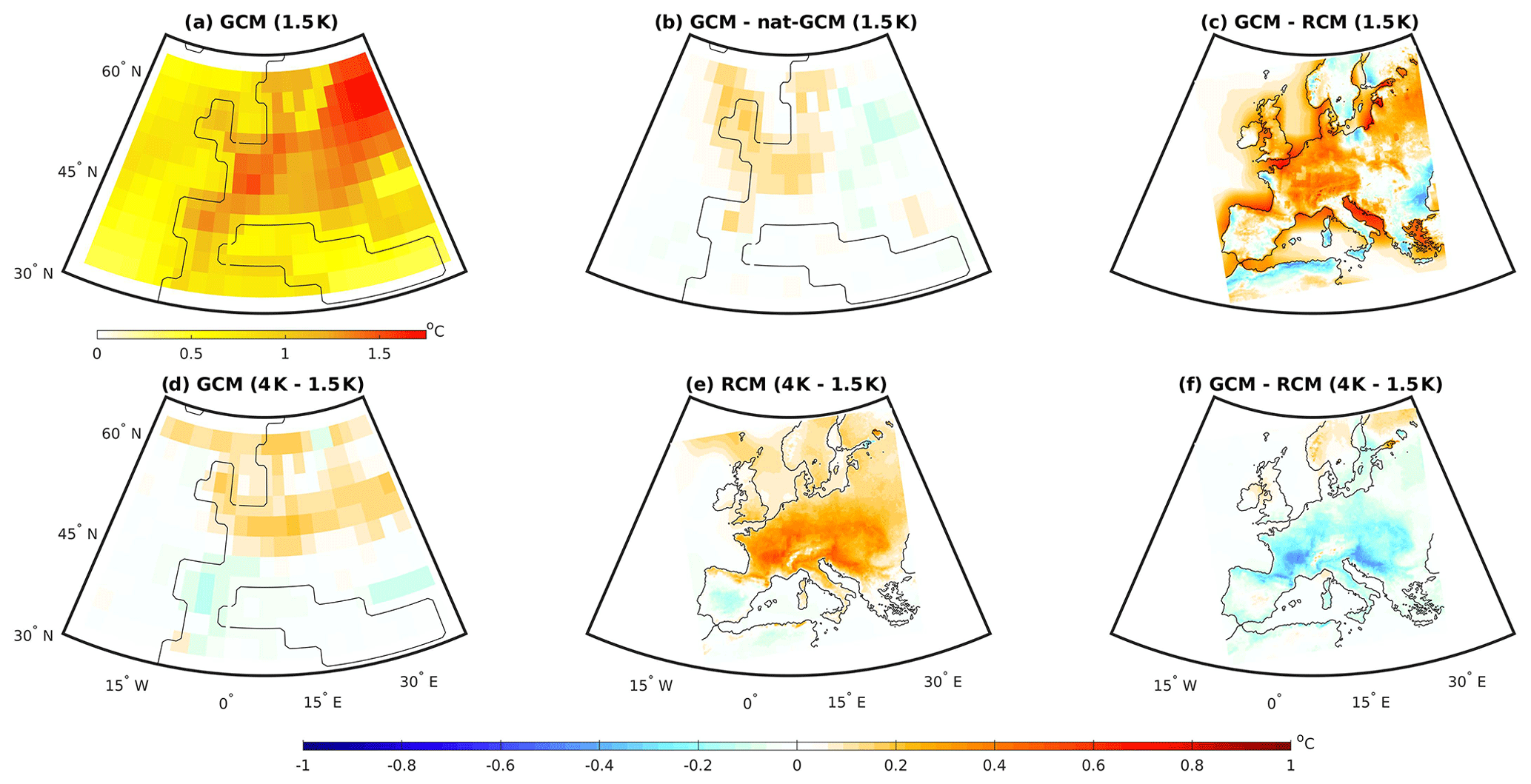
Figure 5 Summer surface air temperature (SAT) variability in (a) the GCM at 1.5 K warming, (b) difference between GCM and the nat-GCM at 1.5 K warming, (c) difference between the GCM and RCM at 1.5 K warming, (d) the GCM at 4 K warming, (e) the RCM at 4 K warming, and (f) difference between the GCM and RCM at 4 K warming. Before the RCM is subtracted from the GCM, the GCM is regridded to the RCM grid. We use an 11-year window around each warming year to analyse the data. SAT variability is calculated as the standard deviation across the pooled summer (mean over June, July, and August each year) SAT from all ensemble members and all years in the time period. The forced response in the mean state is removed by removing the ensemble mean for each summer from each ensemble member prior to the variability calculation. Continental borders are shown for each model's native grid.

Attributing climate responses to volcanic eruptions

By combining the GCM, RCM, and nat-GCM SMILEs we can further investigate the response of both SAT and precipitation to large volcanic eruptions over Europe. To investigate the response to volcanoes previous studies have shown that many ensemble members are needed to tease out the forced response (Maher et al., 2015; Pausata et al., 2015; Bittner et al., 2016; Milinski et al., 2020), meaning that SMILEs are an ideal tool to investigate this question.

By combining the GCM and RCM SMILEs after volcanic eruptions we can investigate the local structure of both the temperature and precipitation responses over Europe to these eruptions. Figure 6 demonstrates that the RCM and GCM give broadly similar response patterns but again that the RCM provides higher-resolution local information. Computationally GCMs are much more efficient than RCMs, making the GCM the perfect tool to run the natural-only forcing experiment with. By using nat-GCM we can precisely tease out which part of GCM and by proxy RCM response is forced by the volcanoes and what the contribution of other factors such as anthropogenic emissions is. The volcanic cooling is underestimated in the GCM and RCM SMILEs when using the standard method of removing the 5-year mean prior to the eruption, particularly in summer (e.g. Fischer et al., 2007; Maher et al., 2015; Liu et al., 2018; Zuo et al., 2018), as is demonstrated by the much stronger cooling found in the nat-GCM SMILE. This demonstrates that using nat-GCM adds to the GCM analysis by better identifying the full cooling response to volcanic eruptions. By using the nat-GCM we can conclude that cooling occurs in both the first summer and winter after the eruptions with more cooling occurring in summer. When considering the precipitation response, there is a general increase in the nat-GCM in summer and a decrease in winter over the domain. The non-volcano response is fairly similar in the two seasons leading to an amplification of the winter pattern and a damping of the summer pattern in the GCM and RCM that can only be identified by combining these SMILEs with the nat-GCM.

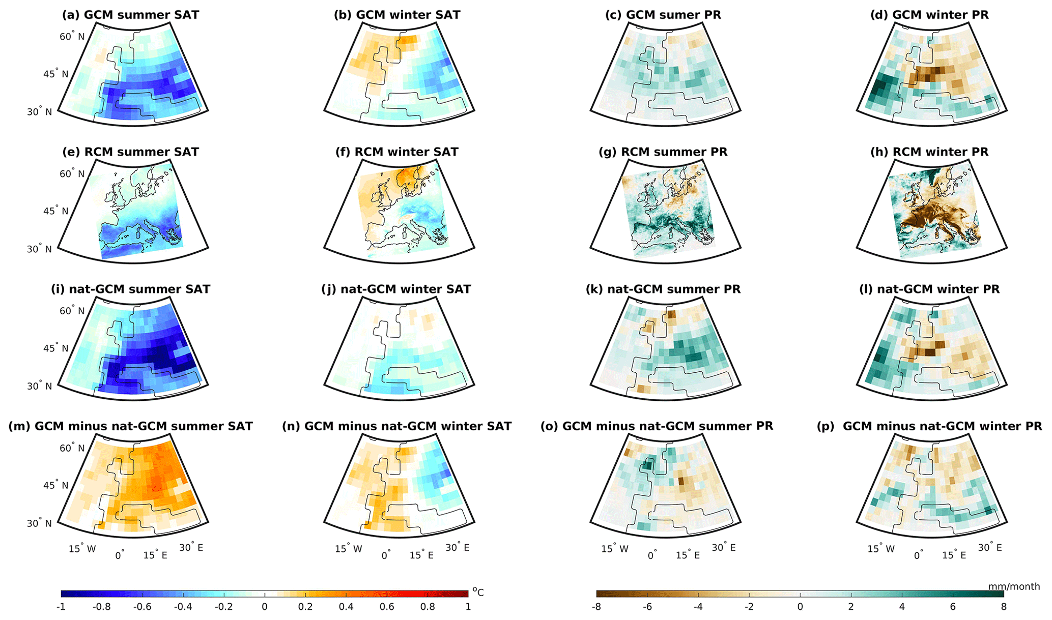
Figure 6 Multi-eruption mean surface air temperature (SAT) for the summer (a, e, i, m) and winter (b, f, j, n) and precipitation for summer (c, g, k, o) and winter (d, h, l, p) 1 year after the eruption. Shown for the GCM (a–d), RCM (e–h), nat-GCM (i–l), and the residual forcing (m–p; GCM minus nat-GCM). Anomalies are shown relative to the 5-year period directly prior to the eruptions. The three eruptions in the multi-eruption mean are Agung, El Chichón, and Pinatubo; the years plotted are 1964, 1983, and 1992 respectively (for winter this is 1963/64, 1982/83, and 1991/92) similar to Fischer et al. (2007). Continental borders are shown for each individual model.

By using nat-GCM SMILE we can investigate these volcanic responses even further. While most previous studies could only look at multi-eruption mean response due to small ensemble sizes (e.g. Maher et al., 2015), we can investigate individual eruption responses in nat-GCM (Fig. 7). We find that El Chichón and Pinatubo have qualitatively more similar responses over Europe, while Agung shows different patterns for both SAT and precipitation. This agrees well with a new study using a different SMILE (MPI-GE) that shows that the intertropical convergence zone and ENSO response is different after Agung due to its aerosol being located in the Southern Hemisphere as compared to the other two eruptions (Ward et al., 2020). By using the nat-GCM we can simply tease out the response over Europe to each individual eruption without needing to remove the anthropogenic signal. Here, using the three SMILEs together gives us additional insight into the European response to volcanic eruptions.

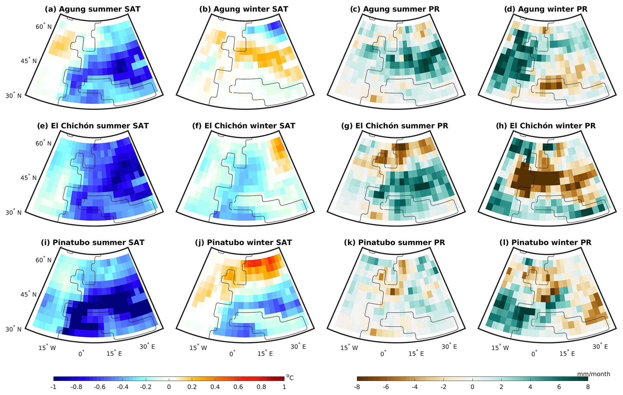
Figure 7 Surface air temperature (SAT) for the summer (a, e, i) and winter (b, f, j) and precipitation for summer (c, g, k) and winter (d, h, l) 1 year after (a–b) Agung, (c–d) El Chichón, and (e–f) Pinatubo shown for the nat-GCM. Anomalies are shown relative to the 5-year period directly prior to the eruptions. The years plotted are 1964, 1983, and 1992 respectively (for winter this is 1963/64, 1982/83, and 1991/92) similar to Fischer et al. (2007). Continental boundaries are shown for the GCM native grid.

4 SMILEs – new frontiers in climate science

The utility of different types of SMILEs has been highlighted in the studies published in this special issue, “Large Ensemble Climate Model Simulations: Exploring Natural Variability, Change Signals and Impacts”. Lehner et al. (2020) demonstrate where and when internal variability is most important for projections using seven GCM SMILEs. Böhnisch et al. (2020) show that RCM SMILEs are important due to the large range of results that can be obtained in single realisations, with von Trentini et al. (2020) finding that it is important to have multiple RCM SMILEs due to the combined role of both internal variability and model differences in causing the uncertainty that occurs on the regional scale as well as the global scale. Examples that use SMILEs to drive a hydrological model, event attribution large ensembles, and a combination of data-assimilated, initialised, and long-term large ensemble simulations and their utility are given by Champagne et al. (2020), Shiogama et al. (2020), and Ehmele et al. (2020) respectively, with Champagne et al. (2020) demonstrating how important SMILEs are for investigating the range of projections we may observe and Ehmele et al. (2020) highlighting the benefit of SMILEs for improving the estimation of extreme values.

While Deser et al. (2020) have demonstrated the utility of having comparable GCM SMILEs from different models, in this editorial we build on this to show the value of having multiple types of SMILEs. We use three types of SMILE (GCM, RCM, and nat-GCM), which all stem from the same modelling chain. While there is a wealth of literature on the added value of RCMs to GCMs that demonstrates that RCMs are most valuable when looking at smaller-scale projections around land–sea regions and orography as well as short-timescale events (Rummukainen, 2016), RCM SMILEs have only recently begun to be utilised in the literature. Single-forcing SMILEs (such as nat-GCMs) have been used more extensively to focus on and identify the role of individual forcings in driving specific events or changes (e.g Kirchmeier-Young et al., 2017; Gagné et al., 2017a, b; Pendergrass et al., 2019) but could be increasingly used in combination with other types of SMILEs, such as RCMs.

By using SMILEs we are able to precisely quantify the forced response, and internal variability in an individual model. By combining this key advantage with the three different types of SMILE we have shown that the European SAT and precipitation responses are non-linear with global warming, with the southern European and local-scale non-linearity in precipitation only identifiable using the RCM SMILE in combination with the driving GCM SMILE. We have investigated individual cities under different levels of warming and identified that the internal variability in precipitation can be quite different in the RCM compared to the GCM, demonstrating the added value of the RCM SMILE at local scales. By using SMILEs we have also been able to quantify forced changes in the summer SAT variability itself. Combining the GCM, RCM, and nat-GCM we have shown where changes in variability can be attributed to increasing greenhouse gas forcing and that the RCM has a larger increase in variability over Europe than the GCM. Finally using all three SMILEs we have investigated the European response to volcanic forcing. In this case the RCM provides a better-resolved response locally but the nat-GCM gives the most additional value and allows us to identify the response to the each eruption individually, while the GCM shows how this volcanic forcing combined with global warming impacts what could be observed.

Here, we have shown that dynamically downscaling a GCM SMILE provides valuable additional information, particularly at local scales compared to the GCM. The computationally cheaper GCM is needed to run the RCM and to compute the warming levels. It also has the advantage that additional sensitivity experiments are affordable. With the modelling chain of GCM, RCM, and targeted GCM (e.g. nat-GCM), we can better interpret some of the signals in the RCM, thus utilising the unique power of the RCM and targeted GCM experiments.

With the many SMILEs now becoming available, new studies that combine different types of ensemble will increasingly be able to answer unsolved questions in climate science, particularly focusing on separating and quantifying the forced response to external forcing and internal variability. Additionally due to the large computational expense of SMILE experiments, utilising the data available and combining experiments is more accessible to many users. Using simple examples and a small subset of the data available, in this editorial we have shown some interesting applications of combining multiple types of large ensemble. Future studies will be able to go well beyond this and push the boundaries of our understanding of internal variability and the forced response to external forcing at both global and local scales due the wealth of new data that has become available. The new methods published in the special issue already begin to push the boundaries of what can be done using large ensembles (Haszpra et al., 2020a; Lehner et al., 2020; Merrifield et al., 2020; Milinski et al., 2020) as do those that combine different ensemble types (Merrifield et al., 2020; Böhnisch et al., 2020; Champagne et al., 2020) and positively contribute to the new science around large ensemble climate modelling.