Assessment of a full-field initialized decadal climate prediction system with the CMIP6 version of EC-Earth

In this paper, we present and evaluate the skill of an EC-Earth3.3 decadal prediction system contributing to the Decadal Climate Prediction Project – Component A (DCPP-A). This prediction system is capable of skilfully simulating past global mean surface temperature variations at interannual and decadal forecast times as well as the local surface temperature in regions such as the tropical Atlantic, the Indian Ocean and most of the continental areas, although most of the skill comes from the representation of the external radiative forcings. A benefit of initialization in the predictive skill is evident in some areas of the tropical Pacific and North Atlantic oceans in the first forecast years, an added value that is mostly confined to the south-east tropical Pacific and the eastern subpolar North Atlantic at the longest forecast times (6–10 years). The central subpolar North Atlantic shows poor predictive skill and a detrimental effect of initialization that leads to a quick collapse in Labrador Sea convection, followed by a weakening of the Atlantic Meridional Overturning Circulation (AMOC) and excessive local sea ice growth. The shutdown in Labrador Sea convection responds to a gradual increase in the local density stratification in the first years of the forecast, ultimately related to the different paces at which surface and subsurface temperature and salinity drift towards their preferred mean state. This transition happens rapidly at the surface and more slowly in the subsurface, where, by the 10th forecast year, the model is still far from the typical mean states in the corresponding ensemble of historical simulations with EC-Earth3. Thus, our study highlights the Labrador Sea as a region that can be sensitive to full-field initialization and hamper the final prediction skill, a problem that can be alleviated by improving the regional model biases through model development and by identifying more optimal initialization strategies.

1 Introduction

Interest in seasonal to decadal climate predictions has grown in recent years due to their potential to provide relevant climate information for decision-making in different socio-economic sectors (e.g. Suckling, 2018; Solaraju-Murali et al., 2019; Merryfield et al., 2020). Scientifically, climate predictions have provided novel ways of evaluating and comparing climate simulations with observations and improve our understanding of the intrinsic predictability of the climate system, including the key mechanisms operating at interannual to decadal timescales.

On these timescales a large part of the predictable signal of climate variations during the observational period is attributable to changes in external radiative forcings (i.e. changes in the climate system energy balance), which can be of natural (e.g. solar irradiance and volcanic aerosols) or anthropogenic (e.g. greenhouse gas concentrations, land use changes and anthropogenic aerosols) origin. For example, at the global scale most of the surface temperature changes can be explained by the warming trend caused by the increasing atmospheric greenhouse gas concentrations, which are partly compensated for by a parallel increase in anthropogenic aerosols (e.g. Bindoff et al., 2013), and the sporadic cooling episodes that followed the major volcanic eruptions of Mt. Agung (1963), El Chichón (1982) and Pinatubo (1991) (e.g. Ménégoz et al., 2018; Hermanson et al., 2020). Estimates of past changes in these radiative forcings are prescribed as boundary conditions to drive the so-called historical climate simulations, which investigate the influence of the forcings on the recent climate variations. These experiments are continued into the future as climate projections with imposed anthropogenic radiative forcings that follow different theoretically derived socio-economic emission scenarios (O'Neill et al., 2016).

The other main source of predictability originates from internal variability, in particular in the slowly evolving components of the climate system, i.e. the ocean (e.g. Meehl et al., 2009). Besides being driven with external radiative forcings, climate predictions are also initialized from the observed state to put the model in phase with observed internal variability. Predictive skill of real-time forecast systems is assessed by producing retrospective predictions (or hindcasts), which are then contrasted with observations. At seasonal to annual timescales, hindcasts show high levels of predictive skill for El Niño–Southern Oscillation (ENSO) (e.g. Barnston et al., 2019). On decadal timescales, many climate models have also shown the capacity to skilfully predict the Atlantic multidecadal variability (AMV) (e.g. García-Serrano et al., 2015) and, to a lesser extent, the Interdecadal Pacific Oscillation (IPO) (e.g. Mochizuki et al., 2009; Chikamoto et al., 2015; Meehl et al., 2015, 2016). The North Atlantic Ocean, more precisely the Subpolar Gyre, has been identified as a region where different retrospective prediction systems skilfully predict the evolution of sea surface temperatures (SST) and upper-ocean heat content (OHC) (e.g. Pohlmann et al., 2009; Keenlyside et al., 2008; Robson et al., 2018; Yeager et al., 2018), although these same systems show a limited capacity to predict the climate of the neighbouring continents, which might be related to an inaccurate representation of key teleconnection mechanisms (e.g. Goddard et al., 2013; Doblas-Reyes et al., 2013). Encouragingly, a recent study by Smith et al. (2020) has shown that decadal predictions contributing to the Coupled Climate Model Intercomparison Project Phase 6 (CMIP6) can be skilful at predicting the low-frequency variations of the North Atlantic Oscillation (NAO), the leading mode of the winter atmospheric circulation in the Northern Hemisphere (Hurrell, 1996), when considering a large multi-model ensemble. Similarly promising results for predicting the NAO at multi-annual timescales has also been shown for the Decadal Prediction Large Ensemble from the National Center for Atmospheric Research (NCAR) (Athanasiadis et al., 2020). Smith et al. (2020) also conclude that the NAO and the related climate signals over Europe might be more predictable than models suggest and that large ensembles of predictions are necessary as current forecast systems can strongly underestimate the predictable signal (Scaife and Smith, 2018).

To reinforce the inter-comparability of the results and allow for the exploitation of large multi-model ensembles, the decadal climate prediction community has promoted the development of coordinated climate prediction exercises. The Decadal Climate Prediction Project (DCPP; Boer et al., 2016), as part of the Coupled Climate Model Intercomparison Project Phase 6 (CMIP6; Eyring et al., 2016), and building upon CMIP5 (Taylor et al., 2012) and the efforts of previous projects (e.g. SPECS and ENSEMBLES), provides such a framework for addressing different aspects and current knowledge gaps in decadal climate prediction. DCPP-A is the main component and consists of an ensemble of decadal hindcasts, initialized at yearly intervals from 1960 up to 2018 using prescribed CMIP6 external radiative forcings.

A crucial step to maximize the skill of decadal predictions is the realistic initialization of the climate system. It is of major importance to produce physically consistent initial conditions that reflect the observed state of climate as faithfully as possible: in particular, the three-dimensional ocean temperature and salinity fields, which determine the basin-wide density gradients and through them the large-scale ocean circulations and transports, which are essential for predictability on decadal timescales (e.g. Meehl et al., 2014; Brune and Baehr, 2020). However, observational records are sparse in time and space, especially in the deep ocean and before modern instruments (such as ARGO floats) were introduced, which poses a challenge with respect to accurately constraining the initial state from observations. For this reason, a typical approach in climate prediction is to use initial conditions from ocean and atmosphere reanalysis. These are produced with data assimilation techniques that ensure a dynamically consistent estimation of the climate state that takes observational uncertainties into account.

Due to structural errors in climate models and biases in their climatologies, when initialized from the observed state, predictions suffer from initial shocks and drifts (e.g. Magnusson et al., 2012; Sanchez-Gomez et al., 2016; Kröger et al., 2018; Meehl et al., 2014). In this paper, initial shocks refer to abrupt changes that occur soon after initialization as a result of the adjustment of the climate model to the initial state and/or to incompatibilities between the initial conditions of the different components, whereas model drift refers to the mean evolution of the forecasts towards an imperfect mean model climate, which is tightly linked to how systematic model errors develop (Sanchez-Gomez et al., 2016). When their occurrence is consistent across start dates, initial shocks (which are not present in all systems) are part of the drift and can even condition its development. Two main initialization approaches are often used: “full-field initialization”, which uses direct observational estimates to initialize the model (e.g. Pohlmann et al., 2009), and “anomaly initialization”, which imposes the observational estimate anomalies on the model climatology (e.g. Smith et al., 2007; Keenlyside et al., 2008). No clear advantage of one approach with respect to the other has been found in terms of forecast quality (e.g. Magnusson et al., 2012; Weber et al., 2015; Boer et al., 2016). The latter was specifically designed to reduce the forecast drift, as it implies initialization from a state closer to the model climatology. However, incompatibilities between the imposed anomalies and the model variability have been shown to cause dynamical imbalances leading to skill degradation in the predictions (e.g. Magnusson et al., 2012; Hazeleger et al., 2013; Volpi et al., 2017). The occurrence of forecast drifts and biases compromises the quality of the predictions, a problem that can be partly circumvented by correcting the predictions a posteriori – for example, by computing forecast-time-dependent anomalies (e.g. Meehl et al., 2014; Goddard et al., 2013; Choudhury et al., 2017).

With the objective of reducing initial shocks, several decadal forecast centres consider the production of in-house assimilation experiments with the same model or model components used for the forecasts from which the initial states are derived. The simplest and most commonly used assimilation framework consists of producing assimilation runs with individual model components (referred to as “weakly coupled”), typically of the ocean model, as it is the most important for the predictability on decadal timescales (e.g. Sanchez-Gomez et al., 2016; Servonnat et al., 2015). This method may benefit the initialization of an individual model component; however, initialization shocks may occur due to incompatibilities among the initial conditions. For this reason, many forecast centres are moving towards fully coupled assimilation (referred to as “strongly coupled”), which is more technically challenging but assures the physical consistency of the initial conditions of all the components, among other advantages (e.g. Brune and Baehr, 2020). For assimilation, a range of different techniques have been used to produce the reconstructions, from classical nudging approaches based on Newtonian relaxation (e.g. Sanchez-Gomez et al., 2016; Servonnat et al., 2015) to more complex and computationally expensive methods like the ensemble Kalman filter approach (e.g. Counillon et al., 2014; Dai et al., 2020), which take aspects of the observational uncertainty into account.

The aim of this paper is to present and analyse a decadal prediction system within the EC-Earth3 model contributing to the CMIP6 DCPP-A. The paper is organized as follows: Sect. 2 provides a description of the EC-Earth3 forecast system, the initialization approach considered, the skill evaluation metrics and the observational datasets used. In Sect. 3, we characterize the predictive capacity for the surface temperatures and investigate the importance of the initialization on surface temperatures, upper-ocean heat content and several interannual to decadal indices of climate variability, followed by an analysis of the predictive skill in the North Atlantic. This section illustrates that the low skill in the central subpolar North Atlantic appears to be related to a strong initial shock and the subsequent model drift. The final section summarizes the key results and conclusions of this study.

2 Data and methodology

2.1 EC-Earth3 decadal forecast system

All experiments analysed in this study were performed with the CMIP6 version of the EC-Earth version 3 atmosphere–ocean general circulation model (AOGCM) in its standard resolution (Döscher and the EC-Earth Consortium, 2021). Its atmospheric component is the Integrated Forecast System (IFS) from the European Centre for Medium-Range Weather Forecasts (ECMWF), cycle cy36r4, with a T255 horizontal resolution (grid size of approximately 80 km) and 91 vertical levels. The HTESSEL (Hydrology Tiled ECMWF Scheme for Surface Exchanges over Land; Balsamo et al., 2009) land surface scheme is integrated in IFS, and the vegetation fields are prescribed and have been derived from an EC-Earth historical simulation coupled with the LPJ-GUESS dynamic vegetation model (LPJGuess; Smith et al., 2014). The ocean component is the version 3.6 of the Nucleus for European Modelling of the Ocean (NEMO; Madec and the NEMO Team, 2016), which is itself composed of the OPA (Ocean PArallelise) ocean model and the Louvain-La-Neuve sea ice model (LIM3; Rousset et al., 2015), both run with an ORCA1 configuration (a tripolar grid defined for NEMO with a 1^∘ horizontal nominal resolution) and 75 vertical levels. The atmospheric and oceanic components are coupled through OASIS (Craig et al., 2017).

Our decadal prediction system follows the CMIP6 DCPP-A protocol (Boer et al., 2016) and, therefore, consists of 10-member ensembles of 10-year-long predictions initialized every year in November from 1960 to 2018 (referred to as PRED hereafter). To determine the impact of initialization, PRED is compared with an ensemble of 15 CMIP6 historical simulations (1960–2015) (Eyring et al., 2016) continued with the SSP2-4.5 (Shared Socioeconomic Pathway 2-4.5) scenario simulations (2015–2100) (O'Neill et al., 2016) and performed with the same model version as PRED. These experiments (referred to as HIST hereafter) correspond to the CMIP6 members 2, 7, 10, 12, 14 and 16–25, which were all performed at the Barcelona Supercomputing Center (BSC). PRED and HIST are both performed with prescribed CMIP6 radiative forcing estimates (i.e., solar irradiance, and green house gas, anthropogenic aerosol and volcanic aerosol concentrations) for the historical period (1960–2014) and the SSP2-4.5 scenario on the subsequent years (Eyring et al., 2016).

In PRED, the different components (atmosphere, land, ocean and sea ice) have been initialized using full-field initialization. The atmospheric and land initial conditions have been interpolated from ERA-40 reanalysis outputs (Uppala et al., 2005) for the 1960–1978 period and from ERA-Interim (Dee et al., 2011) for the 1979–2018 period. The ERA-Interim land surface fields were replaced by the ERA-Interim/Land offline land surface reanalysis (Balsamo et al., 2015) driven by ERA-Interim surface fields and bias-corrected using precipitation from the Global Precipitation Climatology Project (GPCP, Adler et al., 2018). The ocean and sea ice initial conditions come from a NEMO-LIM reconstruction, forced at the surface with fluxes from the DRAKKAR forcing set v5.2 (DFS5.2 Brodeau et al., 2010) up to 2015 and with ERA-Interim (Dee et al., 2011) thereafter. In this reconstruction, ocean temperature and salinity fields from the ECMWF Ocean Reanalysis System 4 (ORAS4) (Mogensen et al., 2012) are assimilated through a standard surface nudging approach (e.g. Servonnat et al., 2015), using temperature and salinity restoring coefficients of $-\mathrm{40}\mathrm{W}{\mathrm{m}}^{-\mathrm{2}}{\mathrm{K}}^{-\mathrm{1}}$ and $-\mathrm{150}\mathrm{mm}{\mathrm{d}}^{-\mathrm{1}}$, respectively. Even if no direct assimilation of sea ice products is performed, the atmospheric surface fluxes combined with the surface ocean temperature nudging are sufficient to bring the initial sea ice state close to observations (e.g. Guemas et al., 2014). Below the mixed layer, a Newtonian relaxation term is also applied to assimilate three-dimensional ORAS4 temperature and salinity fields. For this, a relaxation timescale that increases monotonically with depth is used, which takes approximate values of 10 d at 1000 m, 100 d at 3000 m and 330 d at 5000 m. Subsurface relaxation is applied everywhere except within the 3^∘ S–3^∘ N band to prevent spurious vertical velocity effects (Sanchez-Gomez et al., 2016).

To generate the 10 members of PRED, different strategies are followed depending on the model component. The ensemble spread for the atmospheric initial conditions is generated by adding infinitesimal random perturbations to the three-dimensional temperature field. For the ocean and sea ice initial conditions, five different reconstructions are performed following the nudging strategy previously described, each assimilating one of the five members of ORAS4. The five ocean and sea ice states generated are combined with two different atmospheric initial conditions each to produce the 10 ensemble members.

All the simulations completed in this study were performed with the MareNostrum 4 supercomputer, hosted at the BSC, using the “Autosubmit” workflow manager (Manubens-Gil et al., 2016), a Python toolbox specifically developed at the BSC to facilitate the production of experimental protocols with EC-Earth. This toolbox can easily handle experiments with different members, different start dates and different initial conditions. Autosubmit is hosted in the GitLab repository of the BSC Earth Sciences Department (https://earth.bsc.es/gitlab/es/autosubmit, last access: 29 January 2021). The scripts to run the model and all subsidiary tools are also included in the GitLab repository under version control, and the tool that generates the perturbations saves the seed employed for each member, both contributing to guarantee the reproducibility of the experiments within the maximum fidelity permitted by the model.

The raw model outputs were formatted following the Climate Model Output Rewriter (CMOR)/CMIP6 conventions to ensure efficient use and dissemination within the scientific community. This was done with “ece2cmor” (https://github.com/EC-Earth/ece2cmor3, last access: 29 January 2021), a Python tool for post-processing and cmorisation developed for EC-Earth3 that was implemented in the Autosubmit workflow. After reformatting, the model data were systematically quality checked with various tools to ensure no missing files and scientific validity. Both PRED and HIST experiments are published on the BSC data node of the Earth System Grid Federation (ESGF) where they are publicly available.

2.2 Observational data for verification

Various datasets are used as reference for estimating the forecast quality of the two EC-Earth3 ensembles HIST and PRED. To evaluate surface temperature, we use the NASA GISTEMPv4 (Lenssen et al., 2019) and the Met Office HadCRUT4 (Morice et al., 2012) gridded temperature anomaly products. Both datasets combine near-surface air temperature (SAT) over land and sea surface temperature over the ocean (SST). For indices related to SST only, we use the Met Office HadISSTv3 (Kennedy et al., 2011). For upper-ocean heat content we use the Met Office EN4.2.1 gridded ocean temperature (Good et al., 2013). For comparing spatial fields with observations, EC-Earth3 predictions and historical simulations are re-gridded to the observational grid in the case of the surface temperature variables corresponding to a $\mathrm{2}{}^{\circ }\times \mathrm{2}{}^{\circ }$ regular grid for NASA GISTEMP4 and a $\mathrm{5}{}^{\circ }\times \mathrm{5}{}^{\circ }$ regular grid for HadCRUT4. Ocean heat content is re-gridded to a $\mathrm{2}{}^{\circ }\times \mathrm{2}{}^{\circ }$ regular grid. Model simulations are masked in regions where and when observations have missing values. The regions with missing values in observations remain similar over the investigated period, especially for NASA GISTEMPv4.

2.3 Forecast drift adjustment and verification metrics

In the full-field initialization approach, models are initialized close to the observed state and as the forecasts progress they experience a drift towards the (imperfect) model attractor. This drift needs to be corrected to prevent systematic errors in the prediction. To avoid drift-related effects, the evaluation of climate predictions against observations is performed in the anomaly space (e.g. Meehl et al., 2014). In this paper, we use the “mean drift correction” method which consists of computing the anomalies relative to the forecast-time-dependent climatology. This implies that the drift is assumed to be insensitive to the background climate state (e.g. García-Serrano and Doblas-Reyes, 2012; Goddard et al., 2013), which might not always hold.

Observed and HIST anomalies are computed with respect to their climatologies. In the case of HIST, it is computed from the ensemble mean. All climatologies are computed for the common reference period from 1970 to 2018. This is the longest period for which predictions at all forecast years (1 to 10) can be produced; thus, this period allows us to compute a climatology that is consistent across the whole forecast range. For forecast quality assessment purposes, we use the longest period available for each forecast year (e.g. 1961–2018 for forecast year 1 and 1970–2018 for forecast year 10) in order to produce the most accurate estimate of the predictive skill in each case. This implies that the skill of PRED and HIST may change with the forecast time as the verification period changes.

To measure the forecast quality we use the anomaly correlation coefficient (ACC) and the mean square skill score (MSSS). The ACC measures the linear association between the predicted mean and the observations, but it is insensitive to the scaling. The MSSS metric takes differences in magnitude into account, as it compares the mean square errors of a given forecast with those from a benchmark prediction (e.g. persistence), both evaluated against observations.

The impact of initialization on predictive skill is first assessed by computing the ACC differences between the decadal hindcasts and historical simulations. These differences are deemed to be statistically significant according to the methodology developed by Siegert et al. (2017), which corrects for the independence assumption when two forecasts are strongly correlated. The MSSS is used as well to evaluate the impact of initialization. To do so, we compute it for PRED, using HIST as the reference forecast to beat. Following Eq. (5) from Goddard et al. (2013),

$$\begin{array}{}\text{(1)}& \begin{array}{rl}& \text{MSSS}(P,H)\\ & ={\displaystyle \frac{{\text{ACC}}_{\mathrm{P}}^{\mathrm{2}}-[{\text{ACC}}_{\mathrm{P}}-({\mathit{\sigma }}_{\mathrm{P}}/{\mathit{\sigma }}_{\mathrm{O}}){]}^{\mathrm{2}}-{\text{ACC}}_{\mathrm{H}}^{\mathrm{2}}+[{\text{ACC}}_{\mathrm{H}}-({\mathit{\sigma }}_{\mathrm{H}}/{\mathit{\sigma }}_{\mathrm{O}}){]}^{\mathrm{2}}}{\mathrm{1}-{\text{ACC}}_{\mathrm{H}}^{\mathrm{2}}+[{\text{ACC}}_{\mathrm{H}}-({\mathit{\sigma }}_{\mathrm{H}}/{\mathit{\sigma }}_{\mathrm{O}}){]}^{\mathrm{2}}}},\end{array}\end{array}$$

where ACC_P and ACC_H are the ACC for PRED and HIST respectively, and σ_O, σ_P and σ_H are the standard deviations for the observations, PRED and HIST respectively.

A positive MSSS value indicates that PRED is more accurate than HIST, whereas a negative value indicates the opposite; however, caution is recommended for its interpretation as MSSS is not symmetric around zero and positive and negative values of the same magnitude are not comparable. The statistical significance of the MSSS is estimated using a random walk test following the methodology developed by DelSole and Tippett (2016).

The terms in brackets in Eq. (1) represent the conditional bias of the predictions (CB). We can, therefore, rewrite the numerator of Eq. (1) in terms of the difference between the squared ACC values in PRED and HIST (ΔACC) and the difference between the respective squared CB values (ΔCB):

$$\begin{array}{ll}{\displaystyle }& {\displaystyle }\text{MSSS}(\mathrm{P},\mathrm{H})={\displaystyle \frac{[{\text{ACC}}_{\mathrm{P}}^{\mathrm{2}}-{\text{ACC}}_{\mathrm{H}}^{\mathrm{2}}]-[{\text{CB}}_{\mathrm{P}}^{\mathrm{2}}-{\text{CB}}_{\mathrm{H}}^{\mathrm{2}}]}{\mathrm{1}-{\text{ACC}}_{\mathrm{H}}^{\mathrm{2}}+{\text{CB}}_{\mathrm{H}}^{\mathrm{2}}}}\\ \text{(2)}& {\displaystyle }& {\displaystyle }={\displaystyle \frac{\mathrm{\Delta }{\text{ACC}}^{\mathrm{2}}-\mathrm{\Delta }{\text{CB}}^{\mathrm{2}}}{\mathrm{1}-{\text{ACC}}_{\mathrm{H}}^{\mathrm{2}}+{\text{CB}}_{\mathrm{H}}^{\mathrm{2}}}}.\end{array}$$

These final two terms in the numerator, which compare different characteristics of the forecasts, will be later used to aid the interpretation of the MSSS results. While the correlation term focuses on phase variability disregarding the signal amplitude, the conditional bias term reflects both the magnitude (amplitude) of the respective time series as well as their linear trends (Goddard et al., 2013).

The spread–error ratio (SER; Ho et al., 2013) has also been used as an indicator of the forecast reliability, which is defined as the ratio between the mean intra-ensemble standard deviation and the root mean square error of the forecast ensemble mean. When the SER is greater (lower) than one, the ensemble is overdispersed (under-dispersed) and the predictions will be under-confident (overconfident).

For data retrieval, loading, processing and calculation of verification measures, the “startR” and “s2dverification” (Manubens et al., 2018) R libraries have been used, which were both developed at the BSC.

2.4 Climate indices and diagnostics

Global mean surface temperature (GMST) is derived by blending the SST over ocean and SAT temperatures over land. This allows for a consistent comparison with the aforementioned NASA GISTEMPv4 and HadCRUT4 observational datasets. The use of GMST over global surface air temperature at 2 m height (GSAT) is particularly favourable when assessing long-term climate trends (e.g. Richardson et al., 2018).

In the Pacific Ocean, to distinguish between seasonal to interannual and decadal variability, we look at the ENSO and IPO respectively. For ENSO, we use the NINO3.4 index, which is defined as the area weighted average over the region from 5^∘ N to 5^∘ S and from 170 to 120^∘ W. For the IPO we use the tripolar Pacific index (Henley et al., 2015), which corresponds to the average of SST anomalies over the central equatorial Pacific (region 2: 10^∘ S–10^∘ N, 170^∘ E–90^∘ W) minus the average of the SST anomalies in the northwestern (region 1: 25–45^∘ N, 140^∘ E–145^∘ W) and southwestern Pacific (region 3: 50–15^∘ S, 150^∘ E–160^∘ W). To describe the decadal variability over the Atlantic Basin, we use the AMV definition from Trenberth and Shea (2006). The AMV is calculated as the spatial average of SST anomalies over the North Atlantic (Equator–60^∘ N and 80–0^∘ W) minus the spatial average of SST anomalies averaged from 60^∘ S to 60^∘ N (Trenberth and Shea, 2006; Doblas-Reyes et al., 2013). In addition to the AMV, we also compute the subpolar North Atlantic (SPNA; 50–65^∘ N, 60–10^∘ W) ocean heat content in the upper 300 m (referred to as SPNA-OHC300 hereafter). As the IPO, AMV and SPNA-OHC300 are decadal modes of variability, we filter out part of the interannual variability by considering 4-year temporal averages along the forecast time (i.e. forecast years 1–4, 2–5, 3–6 …) for these indices.

Likewise, density has been computed using the International Equation of State of Seawater (EOS-80) that refers to the level of 2000 dbar (sigma-2), which is a level that represents the deep-water properties. In addition, the contributions of temperature (sigma-T) and salinity (sigma-S) to density were computed using the thermal expansion and haline contraction coefficients, the latter of which were estimated as the density change (in the EOS-80 equation) associated with a small increase in temperature (0.02 ^∘C) and salinity (0.01 psu) respectively.

All ocean diagnostics have been computed using “Earthdiagnostics”, a Python-based package developed at the BSC.

3 Results

3.1 Characterizing the predictive capacity of surface temperature

3.1.1 Global mean surface temperature

First we compare the predicted GMST evolution for different forecast periods (Fig. 1), estimated by combining SAT over land and SST over the ocean (see Sect. 2). PRED reproduces the observed variability and shows very high ACC skill values: 0.96, 0.97 and 0.95 for forecast years 1, 1–5 and 6–10 respectively (similar values are obtained with comparisons to other observational products like HadCRUT4). As expected, HIST does not capture most of the interannual variability (Fig. 1), as it is largely of internal origin and, therefore, averages out by construction. Nevertheless, HIST shows very high skill (0.94, 0.96 and 0.95 for forecast years, 1–5 and 6–10 respectively) associated with the global warming trend and the cooling episodes in response to the volcanic eruptions of Agung (1963), El Chichón (1982) and Pinatubo (1991). The differences in ACC skill between PRED and HIST are not statistically significant, indicating that the high skill of PRED is mainly associated with the external forcings. When the simulations are detrended (a simple attempt to remove the warming signal), PRED shows higher ACC skill values than HIST, revealing the benefit of the initialization, especially for the earlier forecast years (ACC values of 0.75 and 0.5 in forecast year 1 for PRED and HIST respectively).

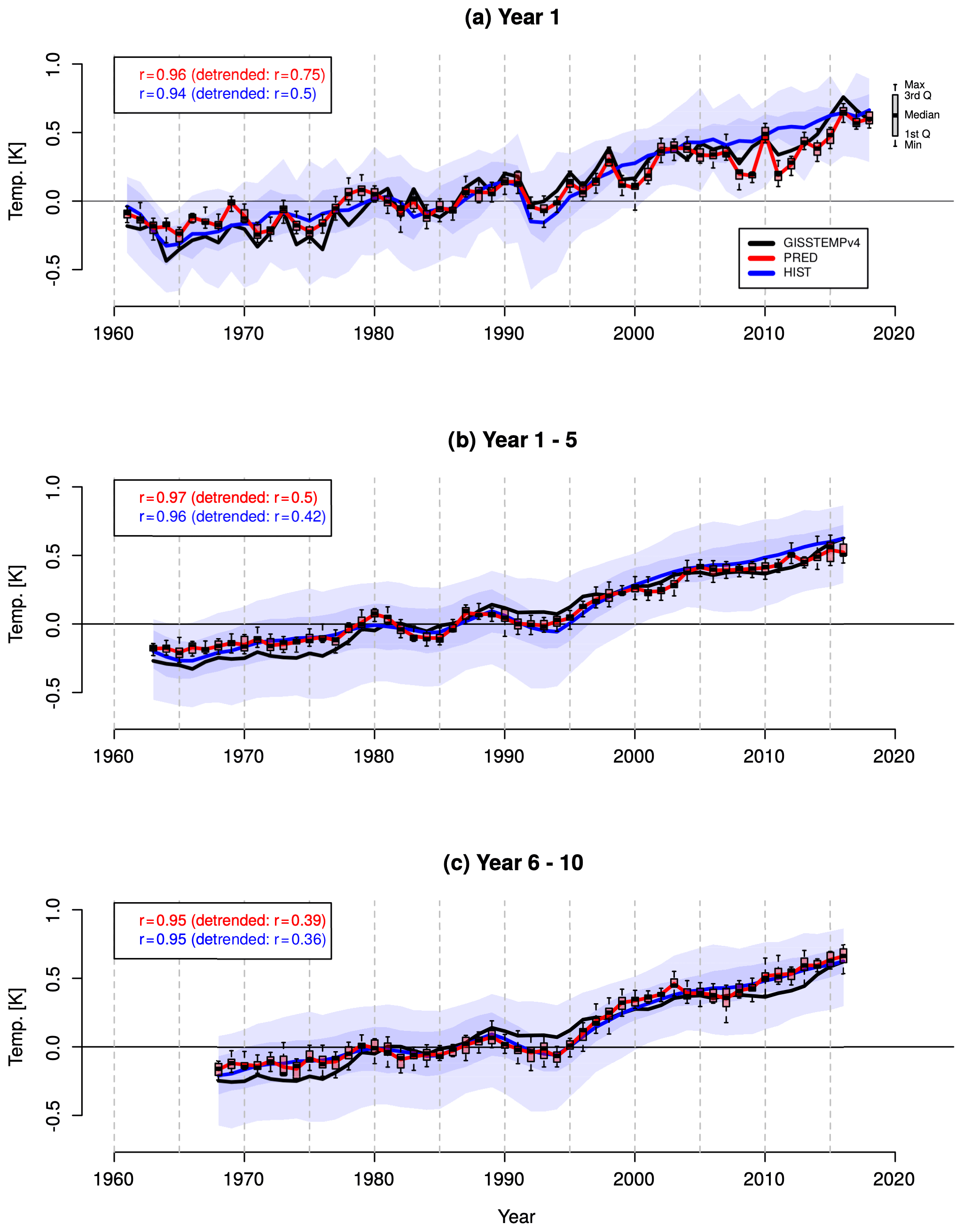
Figure 1 Global mean surface temperature (GMST) annual mean anomaly time series (K) for PRED, HIST (historical+SSP2-4.5) and GISTEMPv4 for (a) forecast years 1, (b) 1–5 and (c) 6–10. The anomalies cover the 1961–2018 period and are referenced to the 1971–2000 mean. Multi-year means (b, c) are plotted on the central year (e.g. 2000 represents the values from 1998 to 2002 in panels b and c). For a fair comparison with observations, PRED and HIST have been masked where and when GISTEMPv4 has missing values. The intra-ensemble spread for PRED and HIST is represented by the box-and-whisker plots and shading respectively. The ACC for PRED and HIST is shown in the top-left corner of each panel, including the ACC after removing a linear trend from the time series (shown in parentheses). All ACC values are statistically significant at the 95 % level.

Comparing the intra-ensemble spread of PRED and HIST (shown by the box-and-whisker plots for PRED and shading for HIST in Fig. 1) shows that PRED has considerably smaller spread even on the longer forecast times. For example, the mean intra-ensemble standard deviation of PRED is 0.05 K, whereas it is 0.20 K for HIST for the first forecast year. This is probably due to the initialization of PRED, which puts the simulated internal and observed variability in phase and may also help to correct systematic errors in the model response to external forcing (e.g. Doblas-Reyes et al., 2013). This difference in spread remains comparable when the ensemble size of HIST is reduced to 10 members, i.e. the same ensemble size of PRED.

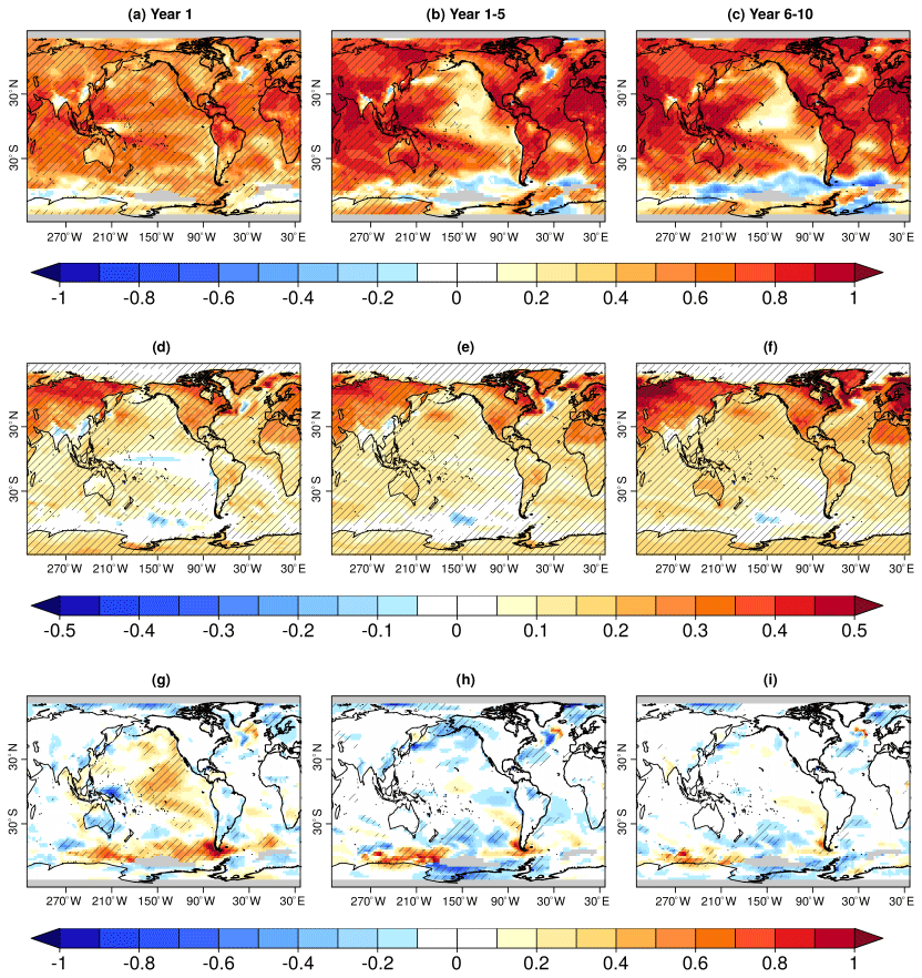
Figure 2 Anomaly correlation coefficient (ACC) for the annual surface temperature (SAT and SST blend) in PRED for forecast years (a) 1, (b) 1–5 and (c) 6–10. The ACC is computed between the model ensemble mean of the blended SAT (over land) and SST (over the ocean) fields and GISTEMPv4. Grid points with missing values in observations are masked in grey. Panels show surface temperature linear trends (in K per decade) in PRED for the same forecast years as in panels (a–c). Panels (g–i) show the ACC difference between PRED and HIST in the same forecast years as above. In all rows, hatching indicates significance at the 95 % confidence level. Both ACC and trends are computed for annual mean values of all available years for the respective forecast period referenced to the 1970–2018 climatology.

3.1.2 Added value of initialization at the regional scale

At the regional level, PRED shows high skill at predicting surface temperature at different forecast ranges (Fig. 2a–c), as expected from the presence of long-term warming trends (Fig. 2d–f). In the first forecast year, most regions show significant skill (Fig. 2a), with a few exceptions such as the central subpolar North Atlantic and some regions of Asia, Australia and the Southern Ocean, where the simulated trends are small and mostly not statistically significant (Fig. 2d). By contrast, the eastern Pacific shows no significant trends but does show significant skill in the first forecast year associated with the initialization of ENSO. On longer timescales (forecast ranges from 1 to 5 and 6 to 10 years) PRED also shows significant skill in many regions worldwide with greater ACC values compared with forecast year 1 (Fig. 2b, c). This is probably a consequence of considering 5-year averages for validation, which reduces the influence of the unpredictable part of interannual variability. There is, however, an important degradation of the skill in some regions for these forecast ranges, in particular in the eastern tropical Pacific, where the model might not be representing the correct ENSO low-frequency variability, and in the North Pacific, where generally low levels of skill have been related to model biases in ocean mixing processes (Guemas et al., 2012). Comparing the forecast periods for years 1–5 and 6–10, two major differences are apparent. First, in the Southern Ocean, skill degrades dramatically with forecast time, which is probably associated with the development of a warm bias due to the incorrect representation of cloud feedbacks in the region (Hyder et al., 2018). Second, the central subpolar North Atlantic seems to exhibit an opposite change in skill, from negative ACC values during the first 5 forecast years to positive but insignificant ACC values in the 5 following years, which might reflect the recovery from an initial adjustment that affects the North Atlantic. This adjustment might be responsible for the strong negative trends over the regions in forecast years 1–5, which are substantially reduced in forecast years 6–10 (Fig. 2e, f). This will be further discussed in Sect. 3.3.

To determine whether there is a benefit of initialization on the surface temperature skill, we compute the difference in ACC between PRED and HIST (Fig. 2g–i) as well as the MSSS of PRED using HIST as the reference forecast (Fig. 3a–c). Moreover, to aid in the interpretation of the MSSS values, we show the two terms that determine its sign, the first being the difference between the squared ACC values of PRED and HIST (Fig. 3d–f), and the second being the difference between their squared conditional biases (Fig. 3g–i). The colour scales in all panels have been adjusted so that red colours represent a contribution to improved skill from initialization (i.e. the colour bar was inverted for the conditional bias plots).

Figure 3 Mean square skill score (MSSS) of the annual mean surface temperature (SAT and SST blend) in PRED using HIST as the reference forecast (see Sect. 2.3) for forecast years (a) 1, (b) 1–5 and (c) 6–10. Hatching indicates where the MSSS is significant using a random walk test (see Sect. 2.3). Its sign is determined by the difference between the terms in panels (d–f) and (g–i) (see Eq. 2). Panels (d–f) show the difference between the squared ACC values in PRED and HIST for the same forecast years. Panels (g–i) show the difference between the squared conditional biases in PRED and HIST for the same forecast years. Note that the colour scale in panels (g–i) is reversed with respect to the other rows so that positive values contribute to improved skill from initialization. GISTEMPv4 is used as the observational reference for all calculations. Annual mean anomalies are computed by masking PRED and HIST with the GISTEMPv4 missing values (masked in grey) and using the common 1970–2018 climatology period.

In the first forecast year, both ACC differences (Fig. 2g) and MSSS (Fig. 3a) show added value from initialization in the Pacific Ocean, the neighbouring region of the Southern Ocean and the eastern subpolar North Atlantic, with MSSS also showing positive impact of initialization in the subtropical Atlantic. The MSSS terms reveal that in the first forecast year, the positive MSSS values (indicative of added value of initialization) are mostly associated with the squared ACC term (Fig. 3d), whereas the squared conditional biases contribute mostly to negative MSSS skill, in particular over the whole SPNA region and the northern North Pacific (Fig. 3g). These negative contributions of the squared conditional bias term are also present at forecast years 1–5, in which both the ACC and MSSS differences become predominantly negative, supporting better predictive capacity in HIST than in PRED and, therefore, indicating that only a few areas, such as the northeastern SPNA and the tropical Pacific (Fig. 3b), are benefiting from initialization. While the skill improvement in the northeastern SPNA is clearly due the higher ACC in PRED (Figs. 2h, 3e), the improvement in the tropical Pacific is due to a reduction in the squared conditional bias of PRED with respect to HIST (Fig. 3h). At longer forecast times (6–10 years), added value from initialization remains very limited. Positive MSSS values are almost exclusive to the eastern tropical Pacific and the southeastern Atlantic, due to a reduction in the squared conditional bias in PRED with respect to HIST (Fig. 3i). In the northeastern SPNA, although the ACC is greater in PRED (Figs. 2i, 3f), the squared conditional bias in PRED is considerably larger than in HIST, leading to very negative MSSS values (Fig. 3i), which suggest that some regional key physical processes (e.g. the gyre and overturning ocean circulations) might not be well represented in EC-Earth3 predictions.

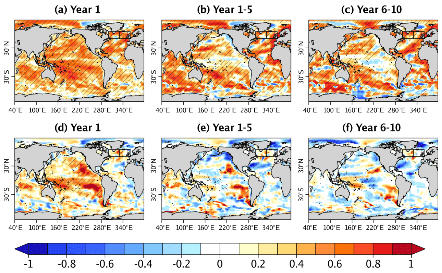
Figure 4 Upper 300 m ocean heat content (OHC300) anomaly correlation coefficient (ACC) of PRED computed with the EN4 observations for (a) forecast years 1, (b) 1–5 and (c) 6–10. The impact of initialization is shown as the difference in ACC between PRED and HIST for (d) forecast years 1, (e) 1–5 and (f) 6–10. In panels (a–c), the hatching indicates the statistical significance of the correlation at the 95 % confidence level. For panels (d–f) hatching indicates the regions where the difference in correlation between HIST and PRED is statistically significant at the 95 % confidence level. The black boxes in the North Atlantic delimit the region over which the SPNA indices have been defined. It also includes the central boundary used to distinguish between its western and eastern sides.

To complement the analysis of surface temperature, we also consider the upper-ocean heat content, a quantity that better represents the thermal inertia of the ocean and a source of decadal variability and predictability for the surface climate (e.g. Meehl et al., 2014; Yeager et al., 2018). As previously shown for surface temperature, in the first forecast year high and significant ACC values are obtained in all major basins for the ocean heat content in the upper 300 m (referred to as OHC300 hereafter; Fig. 4a). A region of negative skill values is evident over the central subpolar North Atlantic, as for the surface temperatures (Fig. 2a). Forecast years 1–5 and 6–10 show that the skill in the tropical and eastern Pacific is lost, as is also the case for some regions in the Atlantic and Pacific sectors of the Southern Ocean (Fig. 4b, c). As for surface temperature, the skill in the central subpolar North Atlantic moderately improves in forecast years 6–10 with respect to forecast years 1–5.

Comparing the ACC difference between the PRED and HIST ensembles reveals that the initialization increases the forecast skill of OHC300 in the eastern subpolar North Atlantic in all the three forecast times (and ranges) considered (Fig. 4d–f); this is a result that is consistent with other forecast systems (e.g. Robson et al., 2018; Yeager et al., 2018). The Pacific Ocean shows significantly improved skill from initialization basin-wide in the first forecast year (i.e. ENSO); however, for forecast years 1–5 and 6–10, the added value of initialization is limited to parts of the eastern subtropical Pacific and the western tropical Pacific. The initialization improves the skill in most of the Indian Ocean at all forecast times considered (although it is not statistically significant for forecast years 6–10), which is consistent with previous studies showing the high skill of decadal predictions in this region (Guemas et al., 2013).

3.2 Skill for the main ocean modes of variability

We further evaluate the predictive capabilities of the EC-Earth3 PRED experiment by considering the skill for predicting several modes of interannual to decadal variability (Fig. 5). In the Pacific Ocean, ENSO is the main mode of climate variability on seasonal to interannual timescales and can help the predictive capacity worldwide through its well-known climate impacts (e.g. McPhaden et al., 2006; Yuan et al., 2018). Figure 5a shows that PRED captures the year-to-year evolution of the observed ENSO, whereas HIST does not; this is due to the dat that ENSO events are out of phase across the HIST ensemble and average out. This is confirmed by the high ACC values during the first 4 forecast months in PRED (ACC>0.9), which are followed by a typical loss of skill that many dynamical forecast systems experience during the spring season (i.e. the spring barrier; Webster and Yang, 1992) and by a recovery in summer through the next winter, in which ACC values remain positive and significant (Fig. 5b). Added value for ENSO due to initialization is evident up to the second forecast year, as indicated by the positive MSSS values and the statistically significant difference in ACC values between PRED and HIST (Fig. 5b). The lack of skill in HIST is expected, because ENSO is barely influenced by the external forcings and the ensemble mean averages the phases of the individual members out. In the predictions, the spread–error ratio reveals that the ENSO predictions tend to be overconfident in the first 2 years, in contrast to HIST which tends to be under-confident. On decadal timescales, the dominant mode of climate variability in the Pacific Basin is the IPO. Figure 5e shows that neither PRED nor HIST is capable of skilfully predicting it – a lack of skill that has been documented in many other prediction systems (e.g. Doblas-Reyes et al., 2013). Nonetheless, initialization does seem to improve the reliability of the IPO (Fig. 5f).

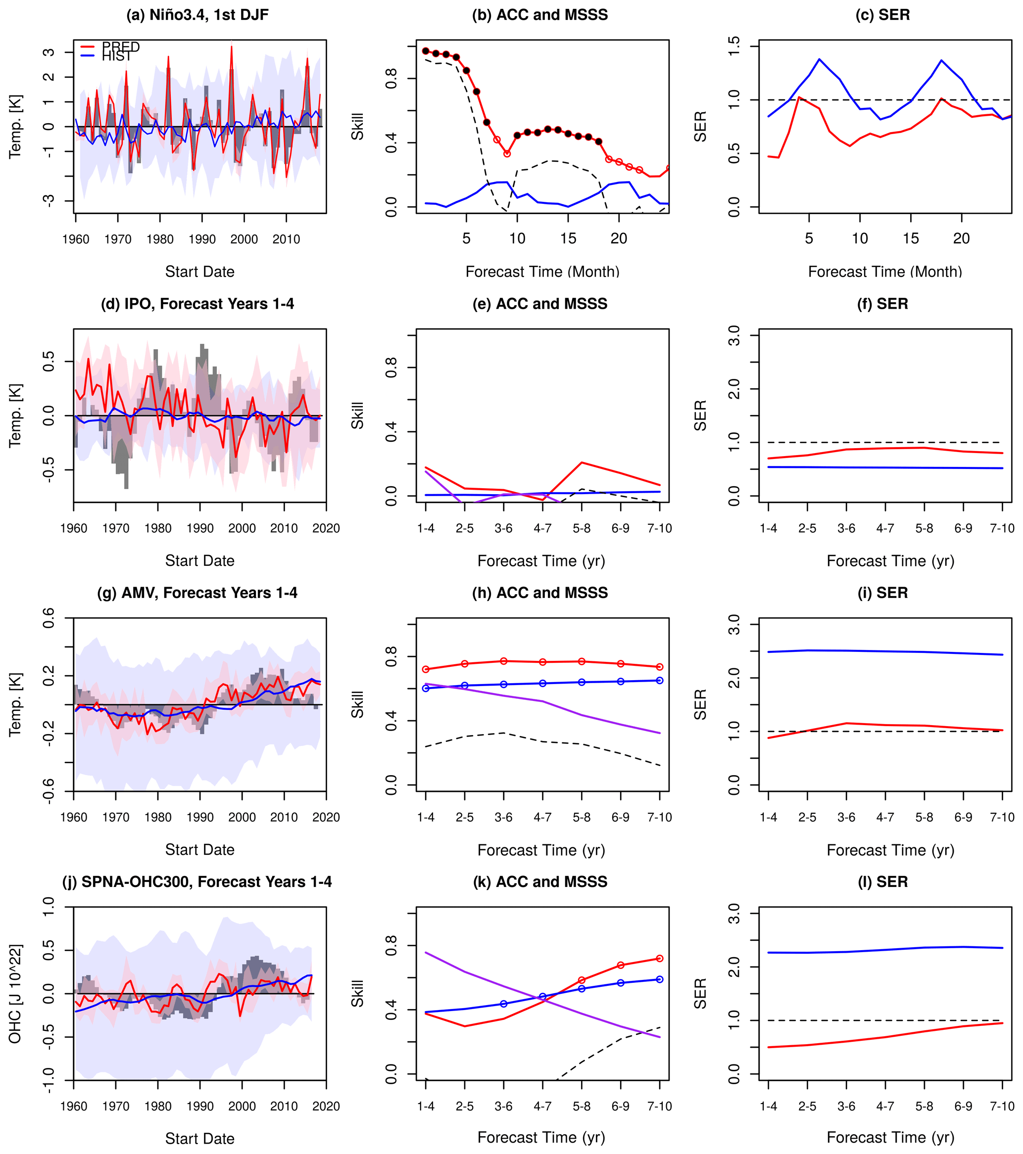
Figure 5 Skill of the selected modes of ocean variability: (a–c) ENSO (Niño3.4 index), (d–f) IPO, (g–i) AMV and (j–l) SPNA-OHC300. Panels (a), (d), (g) and (j) show the observed (grey bars) and predicted (PRED in red and HIST in blue) time series of the indices. The ensemble means are represented using lines, and the ensemble spread is shown using coloured shading. Panel (a) shows the ENSO index for the first winter (DJF), whereas panels (d), (g) and (j) show the average of the first 4 forecast years for the other indices. Panels (b), (e), (h) and (k) show the ACC of PRED (red) and HIST (blue), the MSSS of PRED considering HIST the baseline prediction (black dashed line) and the ACC of a persistence forecast (purple). Statistically significant ACC values (at the 95 % confidence level) are shown using empty circles. ACC differences that are statistically significant (at the 95 % confidence level) between the PRED and HIST are shown using filled circles. Panels (c), (f), (i) and (l) show the spread–error ratio of PRED (red) and HIST (blue).

In the Atlantic Ocean, the AMV is the dominant mode of decadal climate variability and has been linked to several climate impacts over Europe, North America and the Sahel (Zhang and Delwoth, 2006; Sutton and Dong, 2012; Ruprich-Robert et al., 2017, 2018) as well as to Atlantic tropical cyclones (e.g. Caron et al., 2015, 2018). Both PRED and HIST are capable of skilfully predicting the AMV, and they show better performance than a persistence forecast (except for the forecast range from 1 to 4 years in HIST), as shown by the ACC (Fig. 5h). PRED however, is consistently better than HIST, as shown by the MSSS, even though the ACC differences are not statistically significant. The spread–error ratio shows that initialization improves the reliability of the AMV predictions at all forecast ranges (Fig. 5i), as the historical simulations are overdispersive, which is probably due to excessive intra-ensemble spread, as previously described in Sect. 3.1.1.

As the subpolar North Atlantic has been shown to be a region where forecast systems exhibit skill on decadal timescales, we analyse the SPNA-OHC300 index (see Sect. 2.4). As for the AMV, the initialization improves the reliability of the PRED and shows that the HIST intra-ensemble spread may be too large and, therefore, under-confident (Fig. 5l). In terms of predictive capacity, PRED exhibits a lack of skill for the SPNA-OHC300 index up to the forecast range of 4 to 7 years, with significant ACC values emerging for longer forecast ranges, coinciding with the time in which the system outperforms persistence. ACC values in the HIST ensemble (which are not statistically different from those in PRED) also increase with forecast time. In HIST, this is due to the fact that the skill for each forecast range is computed over a different verification period (the same one used for PRED), which used the longest period available for each forecast range. For the longest forecast ranges (e.g. 7–10 years), the first start dates cannot be used, thereby excluding some of the earliest years (e.g. 1960–1966; for which the warming trend was less prominent) and, thus, producing an artificial increase in skill for longer forecast times. Repeating the calculations for PRED over a common verification period to all forecast ranges (i.e. 1970–2018) reveals that lower skill values are still present for the first forecast years (see Fig. S1 in the Supplement), suggesting that the differences in skill with forecast time are not due to differences in the verification period but to other causes. If we determine the skill in OHC300 in the western and eastern SPNA separately (see Fig. S2), we can then see that the skill in PRED is initially poor and then gradually increases reaching significant values in the last forecast years in the western SPNA, whereas the eastern SPNA maintains a high and relatively stable predictive skill. The poor initial predictive skill in the western SPNA might arise from a potential initialization shock, which is a possibility that is discussed in the next subsection. The final skill recovery in the region might be related to the arrival of OHC anomalies from the eastern SPNA, which are slowly advected by the mean gyre circulation.

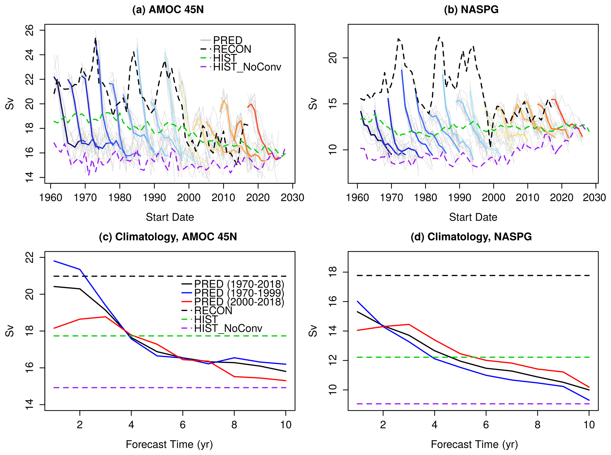
Figure 6 Evolution of the (a) AMOC45N and (b) NASPG in the raw forecasts, historical ensemble and reconstruction. Ensemble mean forecasts (10 members) of PRED are shown from blue to red every four start dates, with individual ensemble members shown in grey. The ensemble mean RECON (5 members) is shown with the black dashed line. The ensemble mean of all HIST (15 members) is shown in green, and the ensemble mean of the HIST members that do not exhibit convection are shown in purple. Panels (c, d) show the PRED climatological values as a function of forecast time for the AMOC45N and NASPG respectively. Three time periods are considered for PRED: the climatology for the 1970–2018 period (black), the climatology for the 1970–2000 period (red) and the climatology for the 2000–2018 period (blue). The black, green and purple dashed lines indicate the climatology computed over the 1970–2018 period for RECON, all HIST members, and HIST members that do not show convection respectively.

3.3 Understanding the limited predictive skill in the subpolar North Atlantic

In the previous section, we have shown the overall detrimental effect of initialization in the EC-Earth3 predictions over some regions of the North Atlantic at all forecast ranges (Fig. 3), leading to lack of predictive skill in the specific case of the central subpolar North Atlantic, as shown by the ACC maps of surface temperature (Fig. 3) and upper-ocean heat content (Figs. 4, 5). Decadal variability in the subpolar North Atlantic is highly influenced by the changes in the ocean circulation, both meridional and barotropic (e.g. Ortega et al., 2017). To understand the role of the ocean circulation, we analyse the evolution of the Atlantic Meridional Overturning Circulation at 45^∘ N (defined as the overturning stream function value at 45^∘ N and at 1000 m depth; referred to as AMOC45N hereafter) and North Atlantic Subpolar Gyre strength index (NASPG, defined as the regional average of the barotropic stream function in the Labrador Sea (52–65^∘ N, 58–43^∘ W), multiplied by minus one to make the values positive so as to aid the comparison) in PRED and HIST (Fig. 6a , b). Additionally, we include the ocean-only reconstruction from which the initial conditions are obtained (referred to as RECON hereafter) to determine how the predictions depart from the initial conditions. Actual model values are used to illustrate how the forecast drift develops. The mean forecast drift is also shown for completeness, estimated as the climatological value as a function of forecast time (Fig. 6c, d). Figure 6 shows that decadal changes in the AMOC and NASPG are highly correlated (e.g. R=0.8 in RECON) – a relationship that has been shown in previous studies (Ortega et al., 2017).

Comparing PRED and RECON allows us to identify several interesting features. In the first forecast year, the predicted AMOC45N is of equal value with respect to RECON, whereas the predicted values tend to be weaker for the NASPG index (Fig. 6). As the forecasts evolve and the model transitions towards its free-running attractor both indices diverge from RECON and experience a pronounced weakening. By forecast year 10, the indices in PRED reach a weaker mean state than in HIST (green dashed lines in Fig. 6c and d respectively). These differences between PRED and HIST suggest either that the forecasts in PRED need to be run for longer to reach their attractor (i.e. HIST) (e.g. Sanchez-Gomez et al., 2016) or that more than one model attractor exists.

For both indices, we also note a clear difference in the way the forecast transitions to the model attractor before and after year 2000. For the first 30 start dates, the AMOC45N and NASPG in PRED start at stronger values than HIST (c.f. RECON values in Fig. 6a and b), and the individual predictions exhibit a fast decline that surpasses the HIST mean state. In year 1995 of RECON, both indices experience a sharp decrease and eventually stabilize around a substantially lower mean state, which is a transition that has been shown to be partly predictable in previous studies (Robson et al., 2012; Yeager et al., 2012; Msadek et al., 2014). Due to this weaker initial state, all predictions after the year 2000 start much closer to the HIST mean state. As a consequence, the drift in PRED is smoother for this period. The fact that there are two distinct periods in which the model drifts in different ways (Fig. 6c, d) may compromise the applicability of the drift correction methods used to compute the forecast anomalies, which assume a stationary forecast drift. This is particularly evident for the AMOC45N, which shows important differences in the PRED climatologies during the first 3 forecast years when the climatologies are computed for the time periods preceding and following the year 2000 (Fig. 6c red and blue lines respectively). Thus, in the case of the AMOC, applying the standard mean drift correction leads to an underestimation of its intensity over the first period and an overestimation over the second period within the first 3 forecast years. In light of this problem, refining the current drift correction techniques to account for this sensitivity to the period and/or initial state considered, or exploring other alternative statistical drift models to recalibrate the predictions (e.g. Nadiga et al., 2019) might help to better estimate the true prediction skill. Interestingly, other variables like the NASPG seem to be less affected by non-stationary drifts (Fig. 6d).

Figure 7 The same as in Fig. 6 but for the mixed layer depth (MLD) in the Labrador Sea in February–March–April (FMA), the sea ice extent (SIE) in the Labrador Sea during the same months and the western SPNA-OHC300 annual mean.

To understand why the AMOC45 and NASPG are not stabilizing in the predictions around the mean HIST state, we focus on the Labrador Sea. The Labrador Sea is a key region of deep-water formation, in which climate models show limitations with respect to representing realistic oceanic convection, which can happen too often, too deep or can be completely absent in some cases (Heuzé, 2017). Figure 7a shows the mixed layer depth (MLD) evolution in the Labrador Sea, which is a proxy for the convection activity in this region. The MLD index is computed as the average of February–March–April, which are the months with the deepest mixing. In PRED, MLD systematically collapses within the first 3 forecast years, which is in stark contrast with the typical behaviour in the HIST ensemble, in which deep convection happens regularly. In the HIST ensemble mean, Labrador convection remains active throughout the whole period, although it exhibits a long-term weakening trend, consistent with the increase in local stratification caused by the externally forced ocean surface warming. The Labrador MLD index also allows us to identify three HIST members with a distinct evolution from the rest, characterized by no convection during most of the historical period with a slight increase from 2005 onward (purple line in Fig. 7a). These simulations have a remarkable similarity to the state towards which PRED appears to be drifting. The ensemble mean of these three HIST members is also compatible with the AMOC45N and NASPG states at the end of the forecasts (purple lines in Fig. 6), suggesting that the attractor towards which PRED converges is associated with a suppressed Labrador Sea convection state. Note also that, in the first forecast year of PRED, the Labrador Sea MLD is stronger than in RECON. All of the above suggest the existence of an initial adjustment in PRED, which initially boosts convection and subsequently brings the model towards a non-convective mean state.

Other key indices are also affected by the Labrador Sea convection collapse in PRED. For example, we see that sea ice grows to occupy the whole Labrador Sea as soon as convection ceases (Fig. 7b, e). As for the MLD, the sea ice extent of the HIST members with no convection is remarkably similar, whereas convection in the other members maintains a relatively reduced sea ice coverage. The western SPNA-OHC300 (50–65^∘ N, 60–30^∘ W) also seems to experience an abrupt initial change, as shown in Fig. 7c; the PRED climatological value at a forecast time of 1 year is lower than in the RECON climatology (Fig. 7f). In forecast years 2–3, this index tends to increase, approaching the HIST mean state, which is higher than in RECON. However, this trajectory changes drastically after forecast year 3 (Fig. 7f), and a quick cooling begins towards the no-convection HIST state. This sudden change could be explained by a delayed response to the convection collapse in the predictions, which is expected to drive a weakening of the SPG intensity by decreasing the density of its inner core and its associated geostrophic current (Levermann and Born, 2007). For all of these indices, we again note that their climatological drifts seem non-stationary (Fig. 7d, e, f) and that predictions started after the year 2000 might not be well bias corrected. This, together with the effect of the strong initial shock, could explain the low (negative) predictive skill in the western SPNA (Figs. 2 4), a region that is key for predicting the NAO (e.g. Athanasiadis et al., 2020), for which PRED also shows low skill (not shown).

3.4 Insights into the Labrador Sea initialization shock and drift

Full-field initialization can sometimes produce strong initialization shocks and drifts, as the climate model adjusts from an initial state that might be substantially far from its attractor (e.g. Sanchez-Gomez et al., 2016). This section focuses on Labrador Sea convection, for which Fig. 7a shows a clear readjustment marked by an initial increase and a subsequent decline. Both aspects of the predicted Labrador Sea evolution are investigated separately. We focus on the preconditioning role of Labrador Sea density stratification on convection and investigate the role of temperature and salinity, two variables that might be experiencing a different initialization adjustment and forecast drift over the region.

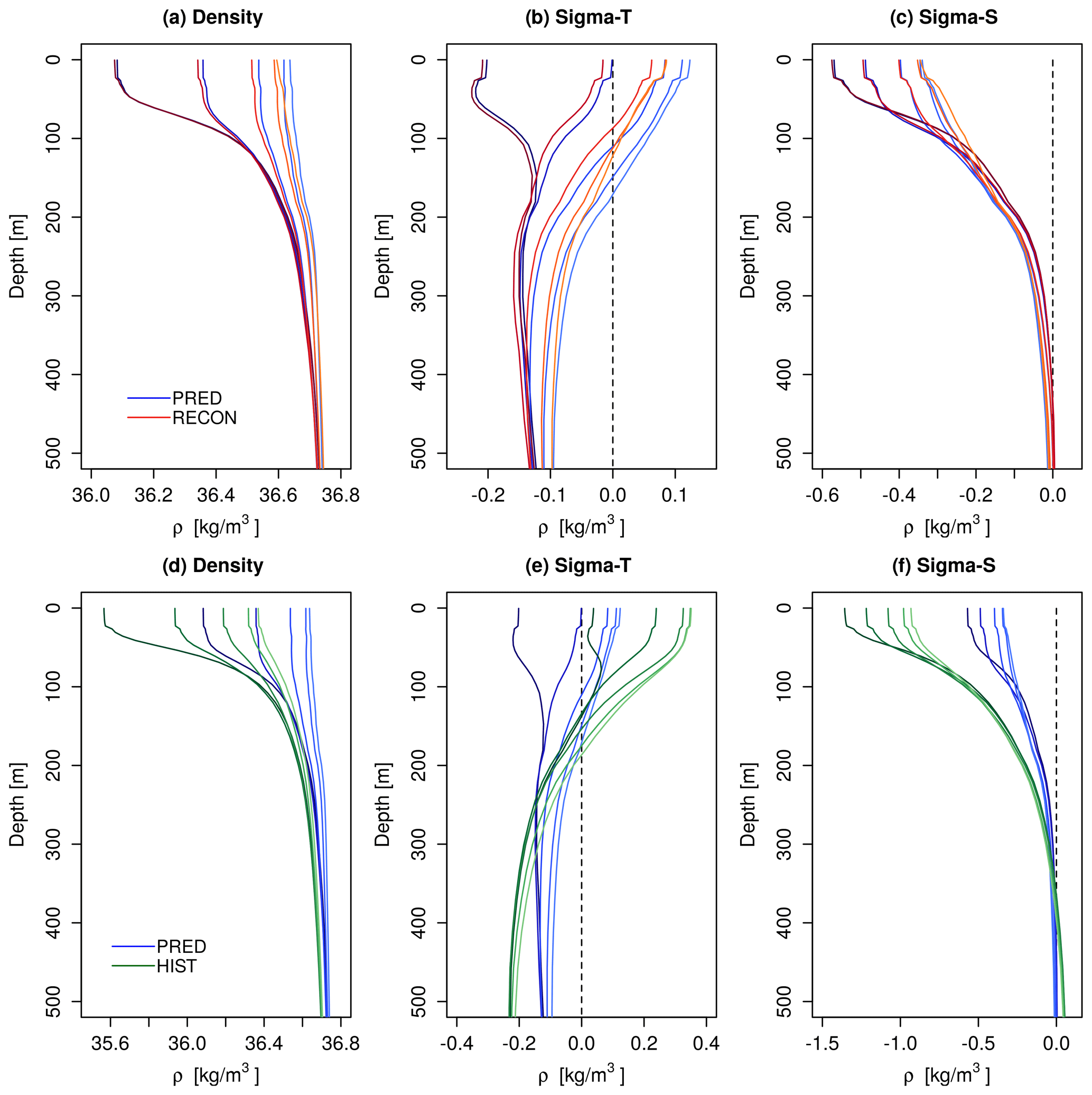
Figure 8 Labrador Sea (a) density, (b) sigma-T and (c) sigma-S climatological profiles in the first 5 forecast months (November–March) of PRED, and the equivalent calendar months of RECON. Panels (d–f) are the same as in panels (a–c) but for PRED and HIST (different panels are used to increase visibility). The colour intensity of the profiles from dark to light refers to increasing the forecast month.

The initial enhancement of convection is explored in Fig. 8, describing the evolution of stratification in the Labrador Sea for the first 5 months of the forecast (November–March). At the time of initialization (November), the density profiles of PRED and RECON are almost identical (dark red and blue lines in Fig. 8a). Differences start to emerge in the subsequent forecast months, in which the density stratification weakens at a different pace, with PRED becoming more weakly stratified and, therefore, more favourable to deep convection. HIST (green lines in Fig. 8d) also shows a similar tendency to reduce density stratification from November to March, although the Labrador Sea density remains more strongly stratified than in PRED and RECON, which would explain why convection is also weaker. By considering the temperature and salinity contributions to density stratification (sigma-T and sigma-S, Fig. 8b, c), we find that even though the overall density structure is dominated by salinity, with temperature largely opposing the mean density stratification, the major differences between PRED and RECON occur in the sigma-T profile and are more notable at the surface. During the first 5 months of the forecast, sigma-T fully accounts for the differences between PRED and RECON in Labrador Sea density (e.g. 0.038 kg m⁻³ at the surface by March), with virtually no differences arising in sigma-S (0.005 kg m⁻³), which fails to counterbalance the temperature-driven changes. As a result, the destabilizing role of temperature on density stratification in the deep convection months is stronger in PRED than in HIST (Fig. 8e, f), promoting deeper convection.

To understand why Labrador Sea stratification diverges from RECON to PRED in the first forecast months, we inspect the local surface restoring fluxes in the former, which, on average, are indicative of systematic model biases in the ocean component. In RECON, the heat-flux-restoring term is consistently positive and, thus, contributes to maintain a warmer surface in these months of deep convection (Fig. 9). These fluxes are not present in PRED because the simulations are fully coupled, which will quickly adjust to a new free-running state with a colder upper Labrador Sea, explaining the relative surface cooling (and associated weakening of density stratification) with respect to RECON (Fig. 8). By contrast, the freshwater fluxes from the salinity-restoring term are negative in the Labrador Sea, and they contribute to maintaining a saltier (and denser) surface in RECON than in PRED. Its effect, however, appears to be small in magnitude, as no remarkable differences emerge in sigma-S between RECON and PRED.

Figure 9 Labrador Sea (52–65^∘ N, 58–43^∘ W) monthly climatology of the nudging correction fluxes in RECON of (a) heat and (b) freshwater. In both cases the fluxes are defined from the atmosphere into the ocean.

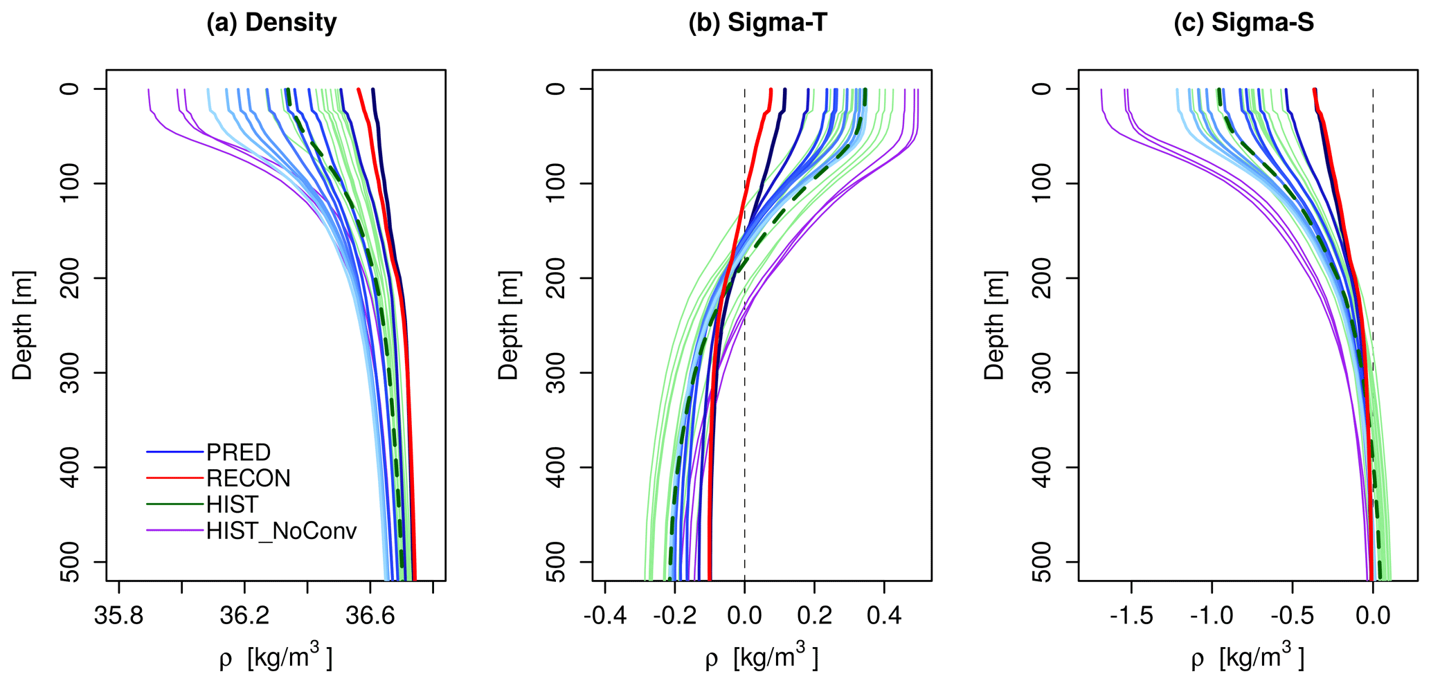
Figure 10 Labrador Sea (a) density, (b) sigma-T and (c) sigma-S climatological profiles for the convection season (February–March–April) in PRED, RECON and HIST. In PRED, the intensity of the blue lines is used to represent the changing forecast time: the darkest blue line corresponds to the 1st forecast year, and the lighter blue line corresponds to the 10th forecast year. The HIST members have been divided into two sub-ensembles: those with and without convection in the Labrador Sea – HIST (green lines) and HIST-NoConv (purple lines). The green dashed line is the HIST ensemble mean using all members.

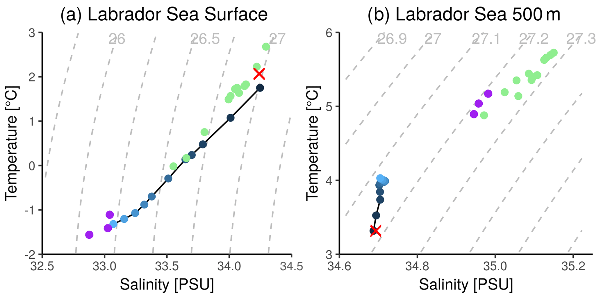
Figure 11 Scatter plot between the climatological Labrador Sea temperature and salinity during the convection season (February–March–April) both (a) at the surface and (b) at 500 m. Blue dots of different intensity represent the climatological PRED values as a function of forecast year: the red cross represents RECON, and the green (purple) dots represent the HIST members with (without) active Labrador Sea convection. Isopycnals are represented by dashed grey lines in the background.

After better understanding the process behind the initial shock in the first winter, we now investigate the origin of the weakening in the Labrador Sea convection after the first forecast year of PRED. Again, we analyse the evolution of the Labrador Sea density profile in PRED, but for each convective season (February–March–April, FMA) as a function of the forecast year (Fig. 10). The corresponding profiles for RECON and the ensemble members of HIST are included to contextualize the predictions. The sigma-T and sigma-S profiles are also shown to disentangle the contributions from temperature and salinity to density. After the first forecast FMA (darkest blue line in Fig. 10), for which we showed a decrease in stratification that favoured deeper convection with respect to RECON, the density stratification becomes increasingly stronger with forecast time. This evolution is explained by the changes in salinity (Fig. 10c), as temperature contributes to decrease stratification at all forecast ranges (Fig. 10b). In the second forecast FMA, density stratification in PRED is already stronger than in RECON (red line in Fig. 10a). By the third forecast FMA, it becomes stronger than in most of the HIST members with active convection (green lines), and by the sixth FMA, it is already higher than in all of them. Interestingly, the stratification of sigma-S is not particularly different in PRED than in the HIST ensemble members with convection, which suggests, once again, that the counterbalancing effect of sigma-T is important to understand the absence of convection in the forecasts. By the 10th (last) forecast FMA (lightest blue line in Fig. 10), the density stratification is remarkably similar to that in the HIST ensemble members without convection. This may suggest that PRED is stabilizing around this particular HIST state. However, this hypothesis is contradicted by the vertical profiles of sigma-T and sigma-S, which appear to be more comparable to the HIST members with convection in the final forecast FMA. Therefore, it is possible that the forecast drift is bringing PRED to a different equilibrium state than in HIST.

To investigate the model drift in the Labrador Sea and how it affects its stratification, we use scatter plots of the climatological Labrador Sea FMA temperature and salinity both at the surface and at 500 m of depth (Fig. 11). At the surface, the mean temperature and salinity for the first forecast FMA remain close to those in RECON, as well as to the values in several HIST members with active convection, all placed along the same isopycnal (27 kg m⁻³). With increasing forecast time, PRED drifts towards a state with lower temperature and fresher conditions – the same one as the HIST members with no convection. During this transition, the surface in PRED also becomes lighter, contributing to increase the stratification in the region. Important differences are observed in the subsurface (i.e. 500 m). For example, unlike for the surface, all the HIST members (i.e. the convective and non-convective ones) show rather similar climatological temperature and salinity (T–S) values, roughly aligned along the same isopycnal (27.25 kg m⁻³). In this case, PRED starts far away from the HIST state (Fig. 11c), although with similar density conditions. The main difference with respect to the surface is that with the subsequent forecast years, the subsurface does not converge towards the typical mean HIST states. By the sixth forecast FMA, the mean temperature and salinity values appear to stabilize along a weaker isopycnal (27.1 kg m⁻³). This suggests that the forecast drift has brought the model to a different equilibrium state, at least in the Labrador Sea. The shock and the later drift may be caused by RECON being far from the EC-Earth3 model climate state in the Labrador Sea subsurface. In particular, in terms of temperature and salinity (Fig. 11), as the mean density profiles are rather comparable due to the compensation between the temperature and salinity contributions (Fig. 10). Similar T–S diagrams, using HIST as a baseline, will be used in the future when evaluating the suitability of different ocean reconstructions to initialize our next decadal prediction systems.

4 Summary and conclusions

In this paper, we have presented and evaluated the predictive skill of a decadal forecast system with EC-Earth, based on full-field initialization, that contributes to the Decadal Climate Prediction Project – Component A (DCPP-A). The main findings of the skill assessment are as follows:

• In agreement with other decadal forecast systems (e.g. Yeager et al., 2018; Robson et al., 2018), EC-Earth3 is able to skilfully simulate the global mean surface temperature at short (forecast year 1) and long (forecast years 6–10) forecast times, with a large part of the skill arising from changes in the external forcings.

• Comparing different skill metrics (i.e. anomaly correlation coefficient and mean square skill score; ACC and MSSS) in the predictions and in an ensemble of historical simulations, we have shown a beneficial effect of initialization. In the first forecast year, surface temperature anomalies in regions like the tropical Pacific, the eastern subpolar North Atlantic and the Southern Ocean show added value from initialization in the predictions. At longer forecast times, only a few localized regions show improvements in terms of MSSS due to initialization, which is exemplified by the eastern equatorial Pacific and the equatorial Atlantic. ACC differences show more limited improvements, from which we highlight a narrow band in the eastern subpolar North Atlantic.

• The added value of initialization is more easily discernible when considering both vertically and regionally integrated ocean quantities. For example, skill maps of the upper 300 m ocean heat content (OHC300), which is more persistent than surface temperature as it is less affected by atmospheric perturbations, show larger areas of improved skill both in the Pacific and Atlantic oceans. Likewise, skill metrics are systematically better in the initialized predictions for the Atlantic multidecadal variability, although the improvements are not statistically significant.

• Another beneficial effect of initialization is the reduction in the ensemble spread in the predictions with respect to the historical simulations, at least for the variables and indices analysed. Therefore, the spread of the predicted anomalies is better constrained at all forecast times.

• In contrast with other studies, the central subpolar North Atlantic is a region of poor forecast skill in the EC-Earth3 forecast system. Both SST and the OHC300 show a detrimental effect of initialization on its regional skill in the first 5 forecast years, which could be explained by an initialization shock and the related long-term drift.

To investigate this potential shock, we have further explored the forecast evolution in a selection of key ocean variables controlling multidecadal variability in the North Atlantic. The analysis showed that Labrador Sea convection collapses by forecast year 3 in the predictions, leading to a rapid weakening of the Atlantic Meridional Overturning Circulation (AMOC) and the Subpolar Gyre circulation. This causes a cooling tendency of the western SPNA and a local expansion of sea ice, which occupies the entire Labrador Sea by forecast year 10. Although a similar state of suppressed convection is found in 3 out of 15 of the historical experiments, the mean of the historical ensemble (which in our case might not exactly correspond to a preferred model state) exhibits higher AMOC and subpolar gyre strength values, regular convection in the Labrador Sea and a more realistic sea ice extent. This suggests that the Labrador Sea convection collapse and subsequent North Atlantic changes are associated with an initialization shock and drift that brings the predictions apart from their expected trajectory as represented by the historical ensemble mean.

We have further related the Labrador Sea convection collapse to the evolution of local density stratification and the separate contributions from temperature and salinity. During the first 3 forecast years, the Labrador density profile becomes more strongly stratified than in most of the historical members with active convection, following an intense surface freshening. This increase in stratification continues with forecast time, approaching but not reaching the strong density stratification levels from the three historical members without convection. To assess if the forecasts actually drift to an attractor characterized by these three historical members, we have additionally evaluated the climatological temperature and salinity in the region as a function of forecast time at the surface and 500 m. At the surface, the predictions start with mean temperature and salinity conditions within the range of those in the historical members with active convection; by the end of the forecast, they approach the typical state of the members without convection. At the subsurface, however, the forecasts remain far from either of the typical historical states, stabilizing at forecast year 10 around a different (and lighter) attractor.

Thus, these results highlight the risk of initializing a sensitive region for decadal prediction, such as the Labrador Sea, too far from its preferred model state; this is a problem that, in this case, could have been minimized by applying a weaker nudging in the subsurface when producing the reconstruction that provided the ocean and sea ice initial conditions. Our findings also underline the importance of reducing the mean model biases in the Labrador Sea as much as possible, in particular at the subsurface. The problems described herein are particularly important when considering full-field initialization (e.g. Magnusson et al., 2012; Smith et al., 2013) – an approach in which initial imbalances of this kind are more likely to occur. In this sense, anomaly initialization emerges as a potential alternative to minimize the drifts and, more importantly here, to minimize the occurrence of initialization shocks. However, as previous studies have shown (e.g. Volpi et al., 2017), this approach is not exempt from problems, and it does not prevent initial model imbalances from happening, whose effect on Labrador Sea convection remains unknown. A complementary alternative is to devote new efforts in climate model development to reduce the model biases over the region and, thus, reduce the mismatches with the observation-constrained products used for initialization. Indeed, an appropriate model tuning in the Labrador Sea would benefit decadal prediction in two ways: first, by improving the model realism in a source region of decadal skill, and second, by helping to prevent or reduce problems associated with initialization.