the Creative Commons Attribution 4.0 License.
the Creative Commons Attribution 4.0 License.
 | 04 Feb 2021
A new view of heat wave dynamics and predictability over the eastern Mediterranean
Sebastian Scher
Julian Quinting
Joaquim G. Pinto
Gabriele Messori
Skillful forecasts of extreme weather events have a major socioeconomic relevance. Here, we compare two complementary approaches to diagnose the predictability of extreme weather: recent developments in dynamical systems theory and numerical ensemble weather forecasts. The former allows us to define atmospheric configurations in terms of their persistence and local dimension, which provides information on how the atmosphere evolves to and from a given state of interest. These metrics may be used as proxies for the intrinsic predictability of the atmosphere, which only depends on the atmosphere's properties. Ensemble weather forecasts provide information on the practical predictability of the atmosphere, which partly depends on the performance of the numerical model used. We focus on heat waves affecting the eastern Mediterranean. These are identified using the climatic stress index (CSI), which was explicitly developed for the summer weather conditions in this region and differentiates between heat waves (upper decile) and cool days (lower decile). Significant differences are found between the two groups from both the dynamical systems and the numerical weather prediction perspectives. Specifically, heat waves show relatively stable flow characteristics (high intrinsic predictability) but comparatively low practical predictability (large model spread and error). For 500 hPa geopotential height fields, the intrinsic predictability of heat waves is lowest at the event's onset and decay. We relate these results to the physical processes governing eastern Mediterranean summer heat waves: adiabatic descent of the air parcels over the region and the geographical origin of the air parcels over land prior to the onset of a heat wave. A detailed analysis of the mid-August 2010 record-breaking heat wave provides further insights into the range of different regional atmospheric configurations conducive to heat waves. We conclude that the dynamical systems approach can be a useful complement to conventional numerical forecasts for understanding the dynamics and predictability of eastern Mediterranean heat waves.
- Article
(14423 KB) - Full-text XML
-
Supplement
(996 KB) - BibTeX
- EndNote


Heat waves are recognized as a major natural hazard (e.g., Easterling et al., 2000), causing detrimental socioeconomic impacts (e.g., “Feeling the heat”, 2018), including excess mortality (e.g., Batisti and Naylor, 2009; Benett et al., 2014; Peterson et al., 2013; Ballester et al., 2019), agricultural loss (e.g., Deryng et al., 2014) and ecosystem impairment (e.g., Williams, 2014; Caldeira et al., 2015). Moreover, heat waves are projected to increase in frequency, intensity and persistence under global warming (e.g., Meehl and Tebaldi, 2004; Stott et al., 2004; Fischer and Schär, 2010; Seneviratne et al., 2012; Russo et al., 2014). The eastern Mediterranean has experienced several extreme heat waves in recent decades (e.g., Kuglitsch et al., 2010), and their frequency and intensity are expected to increase in the coming decades (e.g., Giorgi, 2006; Seneviratne et al., 2012; Lelieveld et al., 2016; Hochman et al., 2018a) upon a background of regional warming and drying (e.g., Barchikovska et al., 2020).
The eastern Mediterranean climate is characterized by wet conditions and mild air temperatures during the winter season and dry and hot weather conditions during summer (e.g., Kushnir et al., 2017). The summer season is characterized by very small inter-daily variability, which is attributable to the dominant and persistent influence of the Persian trough and subtropical high-pressure systems. The interaction between these systems leads to persistent northwesterly winds of continental origin blowing across the Aegean Sea. These winds have been known as “Etesian winds” since ancient times (Tyrlis and Lelieveld, 2013). Together with the Mediterranean Sea breeze, moist air can be transported inland (Alpert et al., 1990; Bitan and Saaroni, 1992) as far as the Dead Sea (Kunin et al., 2019). In the upper levels of the Troposphere, large-scale subsidence is dominant, thereby further hampering the development of clouds and precipitation (Rodwell and Hoskins, 1996; Ziv et al., 2004). In spite of this generally low variability, heat waves are not infrequent during the summer (Harpaz et al., 2014). Still, episodes when the temperature drops to below normal values do occur, some of which are accompanied by summer rains (Saaroni and Ziv, 2000).
Saaroni et al. (2017) detected weaknesses in the ability of earlier synoptic classifications (Alpert et al., 2004a; Dayan et al., 2012) to describe local weather conditions during the eastern Mediterranean summer season. The authors proposed a “climatic stress index” (CSI), which is a combination of the national heat stress index, used operationally by the Israeli Meteorological Service, and the height of the marine inversion base height (see Sect. 2.2). The authors argued that this novel index improves the classification of heat wave days relative to earlier classifications and additionally links directly to the potential impacts.
A notable heat wave in recent years was the 2010 so-called “Russian heat wave”, which caused ∼55 000 excess deaths in eastern Europe and western Russia (e.g., Barriopedro et al., 2011; Katsafados et al., 2014). The 2010 Northern Hemisphere summer saw a strong and persistent blocking ridge at 500 hPa over the Middle East and eastern Europe (e.g., Grumm, 2011; Schneidereit et al., 2012; Quandt et al., 2017), leading to unprecedented temperatures at numerous locations (Barriopedro et al., 2011). The eastern Mediterranean and Israel experienced a record-breaking (with respect to temperature) heat wave during mid-August of that year (https://ims.gov.il/sites/default/files/aug10.pdf, last access: 2 November 2020), which interestingly coincided with what is considered the decay phase of the Russian heat wave (Quandt et al., 2019). In fact, the Zefat Har-Knaan station (Table S1; Fig. S1) recorded a temperature of 40.6 ∘C – the highest temperature since 1939 – while the Jerusalem station (Table S1; Fig. S1) logged a remarkable 41 ∘C – the absolute record for this station since 1942. The ability to predict and issue appropriate warnings for these types of events (and more generally weather events lying in the tails of the respective distributions) is of crucial importance to mitigate the impacts on human life, agriculture and ecosystems (IPCC, 2012; Siebert and Evert, 2014; Williams, 2014).
A general framework that allows a quantitative understanding of processes leading to extreme temperatures during heat waves is that based on Lagrangian backward trajectories. In this framework, the temperature of an air parcel increases by (i) adiabatic warming related to descent and (ii) diabatic heating including latent and sensible heat fluxes, short-wave radiation and long-wave radiation (Holton, 2004). Recent studies have revealed that extreme temperatures during heat waves are most often a combination of adiabatic warming related to descent and diabatic heating near the surface (e.g., Black et al., 2004; Bieli et al., 2015; Santos et al., 2015; Quinting and Reeder, 2017; Zschenderlein et al., 2019). The adiabatic warming is typically associated with upper-level ridges, which promote subsidence. The strongest diabatically driven heating does not necessarily occur at the location of the heat wave itself but rather in geographically remote regions (e.g., Quinting and Reeder, 2017; Quinting et al., 2018; Zschenderlein et al., 2019).
Focusing more directly on the prediction of the evolution of specific atmospheric configurations, which may lead to heat waves, one may consider a partly model-dependent perspective (practical predictability) or a model-independent perspective (intrinsic predictability; Melhauser and Zhang, 2012). The practical predictability is heavily reliant on the availability of initialization data (Lorenz, 1963) and on the correct representation of relevant physical processes in the numerical model being used. However, it also reflects some characteristics of the atmospheric dynamics (e.g., Ferranti et al., 2015; Matsueda and Palmer, 2018). A commonly used method for quantifying the practical predictability is the spread or skill of ensemble forecasts (e.g., Loken et al., 2019).
As opposed to the practical predictability, the intrinsic predictability only depends on the characteristics of the atmosphere itself. However, it is important to note that the atmosphere is influenced and sometimes even controlled by interactions with the land and oceans, albeit mostly at longer timescales than those considered in this study (Entin et al., 2000; Koster et al., 2010; Dirmeyer et al., 2018). Recent developments in dynamical systems theory allow us to quantify the intrinsic predictability of instantaneous atmospheric states using two metrics: persistence (θ−1) and local dimension (d). These reflect how the atmosphere evolves in the neighborhood of a state of interest (Faranda et al., 2017a). High (low) θ−1 (d) implies high intrinsic predictability, whereas low (high) θ−1 (d) suggests low intrinsic predictability. The two forms of atmospheric predictability depend on different factors and, therefore, offer different information. While there is some relation between the two (e.g., Scher and Messori, 2018), one should not expect them to always match for individual cases (Hochman et al., 2020a).
In the present study, we perform a systematic dynamical systems investigation of the temporal evolution of eastern Mediterranean summer heat waves and evaluate whether this may provide insights complementary to a more conventional analysis of the numerical weather forecasts of such events. Specifically, we hypothesize that the dynamical systems analysis captures relevant features of these extremes, such as their persistence, which are not always reflected in the numerical weather forecast. The dynamical systems framework has recently been leveraged for the study of cold spell dynamics (Hochman et al., 2020a).
The paper is organized as follows: Sect. 2 provides a brief description of the methodology, including the used datasets, the CSI index, the dynamical systems and forecast skill metrics as well as the method for backtracking air parcels. Section 3 describes the dynamics of heat waves from both the dynamical system and the numerical weather prediction perspectives and further provides a detailed analysis of the mid-August 2010 heat wave over the eastern Mediterranean as a case study. Finally, Sect. 4 provides the main conclusions and discusses ideas for future research.
2.1 Data
The bulk of our analysis is based on the National Centers for Environmental Prediction/National Center for Atmospheric Research (NCEP/NCAR) Reanalysis project daily and 6-hourly reanalysis data for 1979–2015 (satellite era), on a 2.5∘ × 2.5∘ horizontal grid (Kalnay et al., 1996). Faranda et al. (2017a) showed that the conclusions one may infer from the dynamical systems analysis are generally insensitive to the dataset's horizontal spatial resolution, as long as the major structures characterizing the atmospheric field of interest are resolved. On the contrary, the air parcel tracking (Sect. 2.5) requires data on a relatively high horizontal and vertical grid spacing. Thus, air parcel trajectories are computed from 6-hourly ERA-Interim data for 1979–2015, on a 1∘ × 1∘ horizontal grid and 60 vertical levels (Dee et al., 2011).
The numerical forecasts are acquired from the Global Ensemble Forecast System (GEFS) reforecast v.2 dataset produced by NCEP/NCAR (Hamill et al., 2013). Operational numerical weather prediction (NWP) models are frequently updated. Therefore, archives of operational NWP models are usually inhomogeneous and are consequently not appropriate for studying predictability over long time periods. This problem can be mitigated by using so-called reforecasts. For reforecasts, one fixed version of an NWP model is used in order to create a standardized set of past forecasts. The GEFS reforecast dataset provides a set of daily reforecasts from December 1984 to present. Each reforecast consists of a control forecast and a 10-member ensemble on a 0.5∘ × 0.5∘ grid spacing.
Finally, we make use of a homogenized station dataset over Israel to assess the forecasts. Instrumental meteorological records may be influenced by non-meteorological events, such as station relocation, defects in the instrumentation and environmental changes near the station. The detrimental effects that these may have on the quality of the recorded data can be reduced by homogeneity procedures (Aguilar et al., 2003). Our dataset includes five representative, homogenized stations in Israel with an uninterrupted record of maximum temperatures over 1979–2015 (Table S1, Fig. S1; Yosef et al., 2018).
2.2 Heat wave definition according to the climatic stress index (CSI)
Saaroni et al. (2017) proposed a new index for classifying the summer days over the eastern Mediterranean based on the “environment to climate” approach (Yarnal, 1993; Yarnal et al., 2001). The CSI is comprised of the national heat stress index, used operationally by the Israel Meteorological Service, and the marine inversion base height, which is a major factor influencing the summer weather conditions over the eastern Mediterranean (Ziv et al., 2004). The index suits the identification of heat waves as it does not merely consider the daily temperature but rather additional variables, e.g., humidity and circulation, which directly relate to the impacts of a heat wave on factors such as human physiology (Epstein and Moran, 2006). Saaroni et al. (2017) rigorously evaluated the CSI index with respect to observations and tested a variety of different combinations of predictors, which ultimately resulted in a simple multiple regression equation:
Here, T1000–850 is the average regional lower-level temperature over the region from 31 to 34∘ N and 33 to 37∘ E. Δp is the average sea level pressure over the region from 36 to 44∘ N and 42 to 54∘ E subtracted from the average sea level pressure over the region from 24 to 29∘ N and 33 to 37∘ E, which is an estimate for the intensity of the Etesian winds (see Sect. 1). pIraq represents the average sea level pressure over northern Iraq (35–44∘ N, 46–54∘ E), which is a proxy for the depth of the Persian trough.
The analysis described in the next sections is specifically implemented for extremes of the CSI index, i.e., days during which the CSI exceeds the 90th percentile of the July and August climatological distribution (hereafter referred to as the “upper 10 % of CSI” or heat waves) versus days when the CSI is below the 10th percentile of the July and August distribution (hereafter referred to as “lower 10 % of CSI” or cool days). The onset of a heat wave (cool days) is taken to be the first day on which the CSI exceeds (drops below) the 90th (10th) percentile threshold at 12:00 UTC (0 h in the figures), which ought to roughly match the time of maximum daily temperature. Alpert et al. (2004b) argued that July and August represent the midsummer months, in which the Persian trough occurs on more than 9 d out of 11 d on average. For additional details on the computation of the CSI index and its evaluation, the reader is referred to Saaroni et al. (2017).
2.3 Dynamical systems metrics
We view the atmosphere as a chaotic dynamical system and leverage a recently developed method combining extreme value theory with Poincaré recurrences (Lucarini et al., 2016; Faranda et al., 2017a) to estimate the dynamical properties of atmospheric states. The temporal evolution of the atmosphere can be represented as a long trajectory in a suitably defined phase space. When we use temporally discretized data, such as reanalysis data, we are effectively sampling this trajectory with a given time period, for example 6 or 24 h. An example would be analyzing daily latitude–longitude maps of sea level pressure (SLP) over the eastern Mediterranean (technically a special Poincaré section of the full dynamics): each 2-D map corresponds to a single point along the aforementioned trajectory, for which we seek to compute instantaneous (in time) and local (in phase space) properties. We specifically consider two metrics, which describe instantaneous atmospheric states: the local dimension d and the persistence θ−1. In order to compute the local dimension and persistence for a given state of interest ξ, which in our example would correspond to a specific SLP map in our dataset for a dynamical system with trajectory x(t), we first define logarithmic returns as follows:
where dist is the Euclidean distance between two vectors. Thus, we define g such that it is large when the system is in states close to ξ and small when the system is in states far from ξ. In other words, g is large whenever the SLP map on a given day resembles the SLP map of the day corresponding to the state of interest ξ.
We next consider all cases in which g exceeds a high threshold s(q,ξ), where q is a high quantile of the series g itself. Here, we select q to be the 98th percentile of g. For these cases, which correspond to days whose SLP map is very similar to that of ξ, we can then define exceedances as
Given g above the threshold, we compute how far g is above the threshold. The cumulative probability distribution F(u,ξ) of these exceedances converges to the exponential member of the generalized Pareto distribution (GPD; Freitas et al., 2010; Lucarini et al., 2012). In other words, given a sufficiently long series of SLP maps, we know that the exceedances u computed from these maps obey the following:
Here, ϑ is the extremal index (Moloney et al., 2019), which we calculate using the Süveges maximum likelihood estimator (Süveges, 2007), and u and σ are parameters of the distribution, which depend on the chosen ξ. The local dimension is then obtained as follows:
Persistence is given by
where Δt is the time interval between successive time steps in our dataset. In practice, we choose each SLP map in the dataset in turn as state of interest ξ, which enables us to obtain a value of d and θ−1 for each time step in our dataset.
In practical terms, d reflects the geometry of the trajectories in a small region (neighborhood) of the system's phase space around the state of interest. It is, therefore, related to the number of active degrees of freedom that the system can explore about the state. In other words, it provides information on the way the system evolves around the state of interest, and a higher d will correspond to a less predictable evolution of the system. The persistence θ−1 quantifies how long the system resides in the neighborhood of the state of interest. An infinite persistence implies a fixed point of the system, such that all successive time steps bring no change to the state of the system. At the opposite end of the spectrum, 1 corresponds to a nonpersistent state of the dynamics. The dynamical systems persistence tends to be very sensitive to small changes in the state of the system. In atmospheric sciences, persistence is often computed as the residence time of the atmosphere within a given cluster of states. For example, when computing the persistence of weather regimes, one usually counts how long the atmosphere remains within one given weather regime cluster. However, there are typically a small number of clusters, such that each one contains a relatively large fraction of the total number of time steps within the dataset. In our case, we define recurrences based on a high threshold such that only a small fraction of time steps within our dataset qualify as recurrences. Thus, by design, θ−1 is more sensitive to small changes in the atmosphere than the conventional definition of persistence of weather regimes. The two are, nonetheless, related, and relative differences in θ−1 often reflect relative differences in more conventional atmospheric persistence metrics (Hochman et al., 2019).
The above derivations hold under a specific set of conditions, which are seldom satisfied by climate, or indeed any real-world datasets – such as having infinitely long time series. However, there are both formal (Caby et al., 2020) and empirical (Messori et al., 2017; Buschow and Friedrichs, 2018) results, which support the application of this framework to natural data. In particular, Buschow and Friederichs (2018) have shown that d successfully reflects the dynamical characteristics of the atmosphere even for datasets where the universal convergence to the exponential member of the GPD is not achieved. Messori et al. (2017) further showed that the persistence estimates for atmospheric data issuing from the Süveges estimator are very stable under bootstrap resampling of the intra- and inter-cluster times (i.e., the residence times of the trajectory within and outside the neighborhood of the state of interest). For more details on the estimation of the dynamical systems metrics, the reader is referred to Lucarini et al. (2016) and Faranda et al. (2017a, 2019a).
The dynamical systems perspective has been fruitfully applied to a range of geophysical and other datasets (e.g., Faranda et al., 2019b, c; Brunetti et al., 2019; Faranda et al., 2020; Hochman et al., 2020b; De Luca et al., 2020a; Pons et al., 2020). It has also been explicitly shown that d and θ−1 can offer an objective characterization of synoptic systems over different geographical regions, including the Mediterranean (Hochman et al., 2019; De Luca et al., 2020b), the North Atlantic (Faranda et al., 2017a; Messori et al., 2017; Rodrigues et al., 2018) and the full Northern Hemisphere (Faranda et al., 2017b). In this study, we compute d and θ−1 for daily and 6-hourly 500 hPa geopotential height (Z500) and SLP fields from the NCEP/NCAR Reanalysis, over the eastern Mediterranean, placing Israel in the middle of the domain (27.5–37.5∘ N, 30–40∘ E; Fig. 1). To understand the differences between heat waves and cool days, we analyze both the CDFs (cumulative distribution functions) and the mean temporal evolution of the two groups of days in terms of d and θ−1. The Wilcoxon rank-sum (comparing the medians) and Kolmogorov–Smirnov (comparing the CDFs) tests are used for estimating the differences between the upper and lower 10 % of CSI days at the 5 % significance level. A bootstrap sampling test with 104 samples is used to evaluate the 95 % confidence intervals of the mean temporal evolutions.
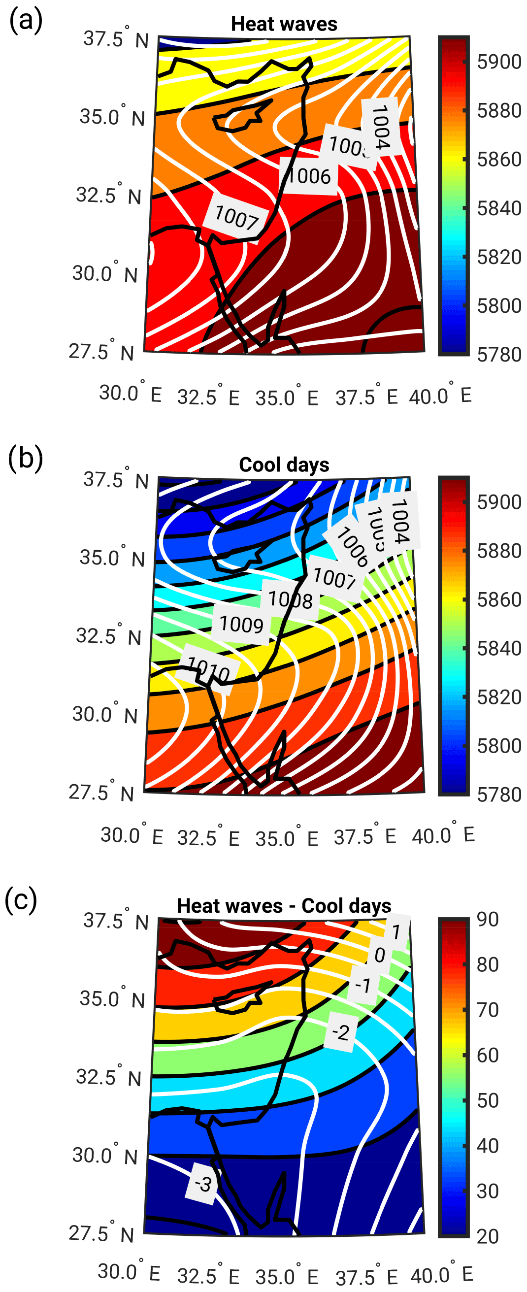
Figure 1Mean sea level pressure (SLP, in hPa, white contours) and 500 hPa geopotential height (Z500, in m, colored shading) for the 10 % of days with the highest (heat waves) and lowest (cool days) climatic stress index (CSI) values: (a) heat wave days mean composite; (b) cool days mean composite; (c) heat waves minus cool days.
Previous studies have shown that the dynamical systems metrics d and θ−1 have a strong seasonal cycle (Faranda et al., 2017a, b; Rodrigues et al., 2018; Hochman et al., 2020a). Thus, we remove the seasonal cycle before comparing the various events. As we are comparing individual days/events during different parts of the summer season, it is better to de-seasonalize the metrics in order to study the anomalies. In other words, we test whether heat waves are synoptically and dynamically unusual with respect to the cool days in the same part of the season. The seasonal cycle is estimated by averaging the metrics for a given time step (e.g., 15 August at 12:00 UTC) over all years, repeating this for all time steps within the year and ultimately smoothing the series with a 30 d moving average.
2.4 Forecast spread and skill
To obtain an ensemble forecast, a set of numerical forecasts are performed with either different initial conditions, and/or perturbation of physical parameterizations. Ensemble forecasts offer an efficient way of estimating uncertainty by computing the ensemble spread. This is quantified by estimating the standard deviation between ensemble members. The spread can be taken as an indicator of practical predictability: in a perfect ensemble, a small spread would generally indicate that we can determine the future weather with a good degree of confidence, whereas a large spread would point towards a larger uncertainty (e.g., Buizza, 1997). This type of approach is commonly used when investigating atmospheric predictability (e.g., Hohenegger et al., 2006; Ferranti et al., 2015), although it does have limitations (e.g., Whitaker and Lough, 1998; Hopson, 2014).
An additional frequently used forecast diagnostic is the absolute error, which provides a measure of forecast skill. The correlation between the ensemble spread and skill of the NWP model indicates the extent to which the ensemble can be used to provide an a priori estimate of the practical predictability of the atmospheric configuration that we are considering. Here, we use the homogeneous station archive mentioned in Sect. 2.1 above as ground truth to estimate the forecasts' absolute error. In order to remove biases due to topographic differences between the model and the stations, the GEFS reforecast gridded data are bilinearly horizontally interpolated to the location of the stations. The bias computed over the whole period is then removed for each station.
The GEFS reforecasts are initialized at 00:00 UTC and are available at 3 h intervals. As our analysis focuses on heat waves, we estimate the spread and skill for maximum temperature and SLP at a lead time of 69 h, and the maximum temperature is defined between 45 and 69 h. Given the 3 h interval of the forecast data, bearing in mind that each station's maximum temperature is recorded between 20:00 and 20:00 UTC of the next day, this time window roughly corresponds to the definition of maximum temperature for the station data. As the dynamical systems metrics offer information on the temporal evolution of the atmosphere in the neighborhood of a given reference state, we argue that using the time of forecast initialization as the temporal coordinate when plotting spread and error is most indicative for comparing the dynamical systems and numerical forecasts. In the Supplement, we also plot the spread and skill for the forecasts initialized 69 h before the marked time. Thus, the plots in the main text show forecast initialization times, whereas those in the Supplement show the forecast valid times. Statistical inference is accomplished by the same tests mentioned in Sect. 2.3.
2.5 Air parcel tracking
In order to identify typical pathways of air masses leading to situations with high and low CSI values, 10 d backward trajectories are computed using the Lagrangian analysis tool (LAGRANTO; Wernli and Davies, 1997; Sprenger and Wernli, 2015). The reader is referred to Fig. 2 in Sprenger and Wernli (2015) for a schematic overview of the typical steps taken to compute trajectories. The tracking of temperature and potential temperature along the trajectory further allows for the quantification of the contribution of adiabatic and diabatic processes to the anomalous temperatures. The vertical and horizontal wind components required for the trajectory computations are acquired from the ERA-Interim reanalysis (Sect. 2.1; Dee et al., 2011). The trajectories are initialized at 12:00 UTC from fixed points in the whole study region on the first day of a heat wave or cool days (Fig. 1). In order to analyze the near-surface air masses, i.e., those related to the hot and cool conditions, we consider trajectories that are initialized between the surface and 90 hPa above the surface. According to recent studies, the planetary boundary layer height in Israel during summer is ∼600–900 m above the surface (Uzan et al., 2016, 2020). Assuming hydrostatic balance and, thus, a pressure decrease of approximately 1 hPa every 8 m height difference, 90 hPa corresponds to about 720 m. Therefore, this can be considered a reasonable choice.
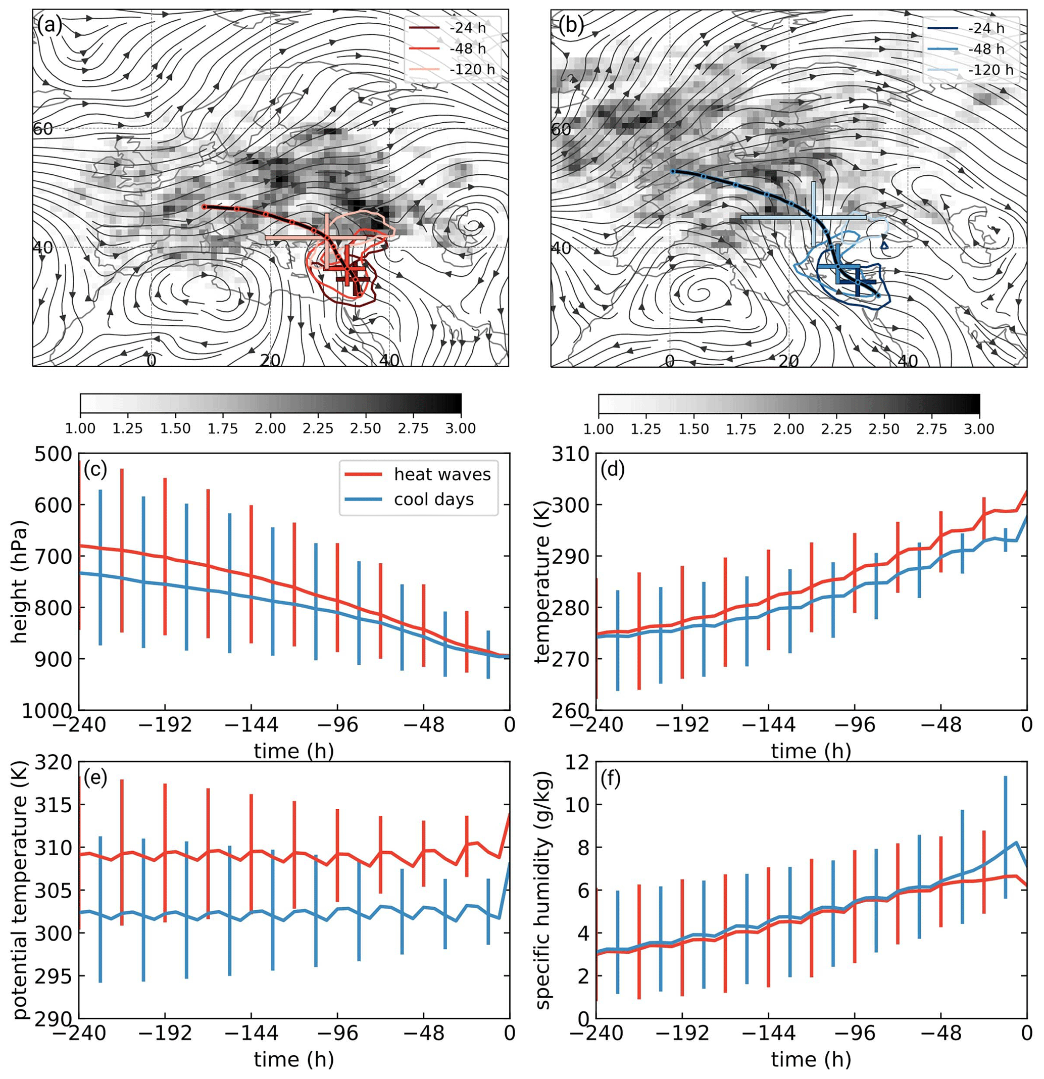
Figure 2Median backward trajectory for (a) heat waves (upper 10 % of CSI) and (b) cool days (lower 10 % of CSI), with circles indicating days (from 10 d before onset to onset). Gray shading shows the trajectory density 10 d before onset (number of trajectories per 1000 km2), and contours show the trajectory density for the indicated time lags (5, 2 and 1 d before onset; contours denote a density of 20 trajectories per 1000 km2). Streamlines of 800 hPa winds averaged between −5 and −1 d are included. The interquartile range of the trajectory positions is shown using crosses for the different time lags. The median evolution of (c) pressure (hPa), (d) temperature (K), (e) potential temperature (K) and (f) specific humidity (g kg−1) of air parcels is also shown. Heat waves are indicated in red, and cool days are shown in blue. The interquartile range is plotted for the physical properties of the air parcels. A value of 0 h corresponds to the first day of CSI ≥ 90 % or CSI ≤ 10 % and at 12:00 UTC.
The trajectories are calculated from 6-hourly ERA-Interim data and remapped to a 1∘ regular latitude–longitude grid. Thus, the analyzed wind field does not resolve sub-grid-scale processes, such as Lagrangian transports due to small convective cells. Also, vertical motion associated with short-lived convection between two time steps is not accounted for. Still, for a climatological investigation, which is the focus of this study, the trajectory calculation is a suitable diagnostic.
3.1 Dynamics of heat waves over the eastern Mediterranean
We first analyze the differences between heat waves (upper 10 % of CSI values) and cool days (lower 10 % of CSI values). From an atmospheric dynamics' standpoint, the main difference between the two groups is that heat wave days are associated with an upper-level ridge, whose center is located in the southeastern part of the study region (Fig. 1a), whereas cool days are associated with an upper-level trough, whose center is located at the northwestern part of the study region (Fig. 1b). The SLP patterns are quite similar in both groups, but the heat waves show lower SLP in the southwest and a higher SLP in the northeast compared with the cool days sample (Fig. 1c). This implies stronger pressure gradients in the cool days' subgroup, leading to enhanced cool air advection from the Mediterranean Sea inland, in comparison to the heat wave days. Furthermore, the abovementioned pattern reveals that the large-scale configuration is an important factor in the generation of a heat wave over the eastern Mediterranean. The backward trajectory air parcel analysis illustrates that the flow preceding an extreme heat wave has a roughly meridional orientation when traveling over the eastern Mediterranean and originates over the European continent (Fig. 2a). On the other hand, the air parcels for cool days often originate over the Atlantic and take a more zonal pathway across the eastern Mediterranean (Fig. 2b). The initial potential temperature of the heat wave air masses is about 7 K higher than that for the cool days (Fig. 2e). The differences in potential temperature between the two groups can mainly be attributed to the more continental origin of the air parcels for the heat waves: these air parcels potentially transport warmer air masses that descend on their path to the target region. Their descent, which is stronger than for cool days (Fig. 2c), is accompanied by a temperature increase of more than 25 K during the 10 d period (Fig. 2d). The potential temperature remains nearly constant until the final stages of the descent except for the diurnal cycle (Fig. 2e). Thus, we conclude that the extreme heat is related to an adiabatic descent of the air parcels over the eastern Mediterranean rather than to diabatic heating. In other words, the warm air parcels are transported towards the eastern Mediterranean with the governing westerlies rather than heated up locally over several days. This supports the findings of Harpaz et al. (2014), who argued that extreme summer heat waves over the eastern Mediterranean are mostly regulated by midlatitude disturbances rather than by the Asian monsoon, as previously proposed by Ziv et al. (2004). An additional important difference between the two sets of CSI events is that, unlike for the heat waves (Fig. 2a, f), the specific humidity of the cool days increases by 2 g kg−1 around h, due to the longer stretch that the latter air parcels follow over the Mediterranean Sea (Fig. 2b, f) and perhaps some enhanced convection, which our analysis does not account for. Indeed, comparing the portion of terrestrial back-trajectories for heat waves and cool days (Fig. S2) suggests that for most of the time they are quite similar. It is only 72–24 h prior to the events that the portion of terrestrial back-trajectories for cool days reaches a minimum and is much lower than for heat waves (Fig. S2).
From a dynamical systems point of view, the upper and lower 10 % of CSI also exhibit substantial differences. Fig. 3 shows a phase plane diagram for d and θ computed on Z500 and SLP for the heat waves and cool days. θ is significantly lower at both levels for heat waves with respect to cool days, i.e., the former are generally more persistent systems. Statistically significant differences in the median local dimensions (d) of the two groups are found only for the Z500 variable, for which the heat waves typically display a lower local dimension (d) than the cool days (Fig. 3a). The clear separation between the two groups, especially at the upper level (cf. Fig. 3a and b) correlates well with the atmospheric dynamics' viewpoint, which also shows more pronounced differences at Z500 (Fig. 1). This points to the importance of using different variables at different pressure levels to obtain a comprehensive picture of the dynamics of heat waves.
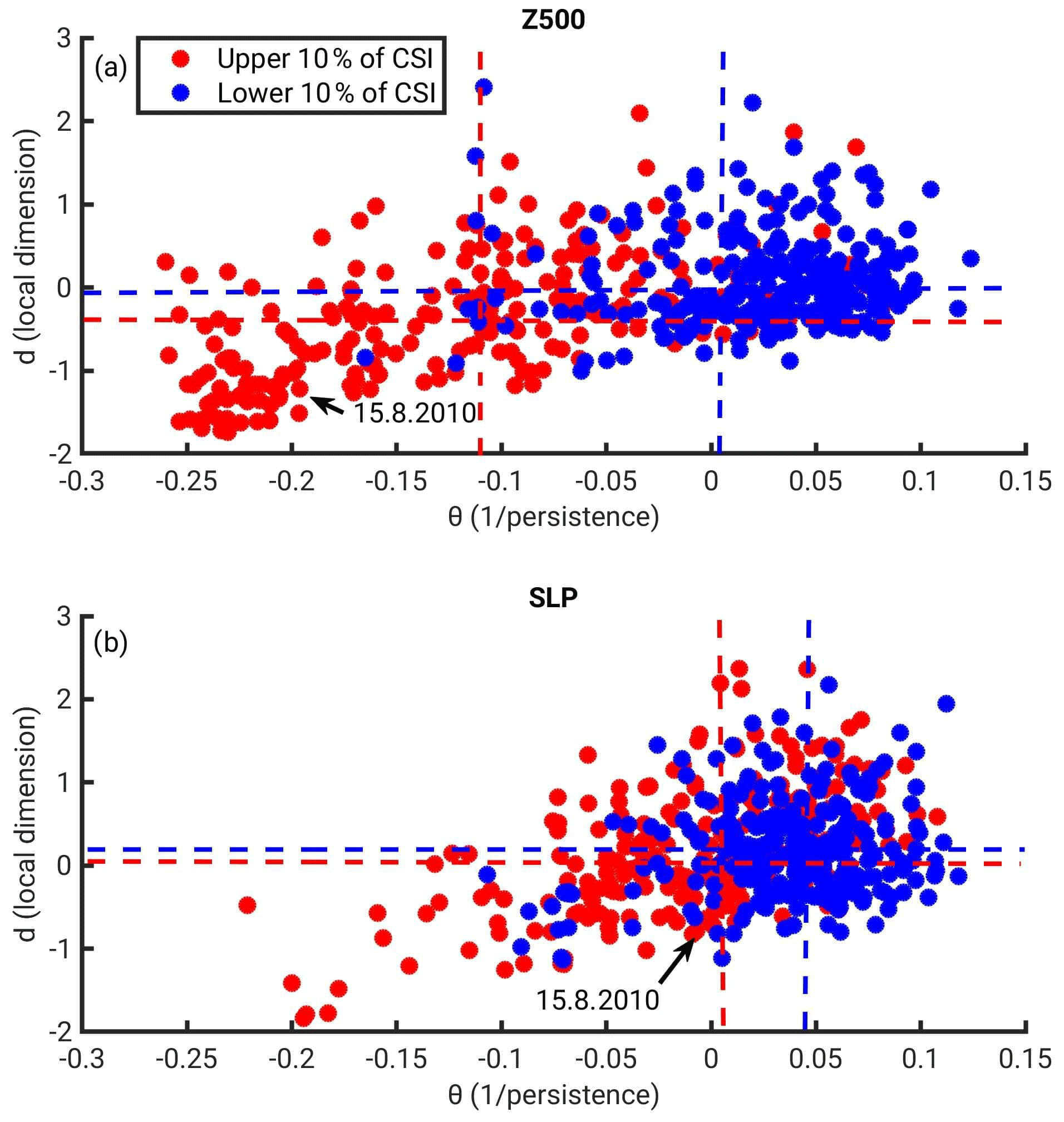
Figure 3A phase plane diagram for the upper and lower 10 % of CSI daily values (heat waves in red and cool days in blue). The de-seasonalized dynamical systems metrics (d and θ) were computed for (a) Z500 and (b) SLP. Dashed lines represent the median values of d and θ. The 15 August 2010 is indicated by the black arrows.

Figure 4The average temporal evolution of the dynamical systems metrics (d and θ) for heat wave (upper 10 % of CSI) and cool day (lower 10 % of CSI) events. The dynamical systems metrics were computed for (a, b) Z500 and (c, d) SLP. The events are centered (0 h) on the first day of CSI ≥ 90 % or CSI ≤ 10 % and at 12:00 UTC. A 95 % bootstrap confidence interval is plotted (shading).
Figure 4 displays the average temporal evolution of d and θ during the selected events, again computed for Z500 and SLP. Zero on the x axis denotes the first day of the event at 12:00 UTC, whereas a value of zero on the y axis implies that the events are not different from the climatology of the days they occurred in. Substantial differences are found between the time evolutions of the upper and lower 10 % of the CSI events. For Z500, the temporal evolution of d and θ for heat waves are in phase with each other and show a minimum with below climatology values in the 24 h preceding the event onset (Fig. 4a). While there is still a considerable spread around the mean, even the upper bounds of our confidence intervals are well below zero in the buildup to the events. Instead, cool days display weak positive anomalies of d and θ, but these are almost never significantly different from zero (Fig. 4b). The dynamical systems metrics computed on SLP provide a completely different picture: heat waves typically display a weak above climatology d, which increases towards the event onset and then decreases (Fig. 4c). θ displays a slightly below climatology persistence (i.e., positive anomalies) and decreases towards the event onset (Fig. 4c). However, the very large spread in the composite evolution, in particular in d, suggests some caution in overinterpreting the details of these evolutions. Cool days are characterized by higher positive anomalies of d and θ in the days preceding the event. The buildup to this type of event is characterized by an increase in θ (decrease in persistence) and a decrease in d (decrease in active degrees of freedom; Fig. 4d). The cool days also appear to have a more coherent evolution (lower spread around the mean) than the heat waves for SLP.

Figure 5Forecast spread and skill for heat waves (upper 10 % of CSI) and cool days (lower 10 % of CSI). The lines show the mean temporal evolution of the ensemble model spread for Tmax (a), SLP (e) and the absolute error for Tmax (c) of forecasts with a lead time of 69 h, initialized at different time lags with respect to the events, calculated every 24 h. The events are centered (0 h) on the first day of CSI ≥ 90 % or CSI ≤ lower 10 % and at 12:00 UTC. The CDFs of the mean ensemble forecast model spread for Tmax (b), SLP (f) and the absolute error of Tmax (d) for the forecasts with a lead time of 69 h initialized at 00:00 UTC. A 95 % bootstrap confidence interval is shown using shading for the temporal evolution plots (a, c, e). The plots are displayed for the time of forecast initialization (see Sect. 2.4).
Thus, the differentiation between the two samples is more pronounced when computing the metrics on Z500 than on SLP (Fig. 4), as also shown in the daily distributions (Fig. 3). Moreover, the variability in the temporal evolution of the dynamical systems metrics is smaller in Z500 than in SLP (Fig. 4). This points to (i) coherent, and very different, upper-level conditions, which engender the two sets of CSI days as well as (ii) a comparatively wide range of possible near-surface patterns leading to severe heat waves. The latter may be explained by the fact that, given initially warm upper-level air parcels and upper-level subsidence leading to rapid adiabatic warming, the occurrence of a heat wave is then relatively insensitive to the details of the surface conditions (e.g., Baldi et al., 2006; Harpaz et al., 2014). Our general understanding of the synoptic conditions at surface levels further suggests that the delicate interplay between the Persian trough and subtropical high systems (Alpert et al., 1990) may contribute to the large spread of both heat waves and cool days regarding the dynamical systems metrics computed on SLP.
We next analyze numerical ensemble forecasts from the GEFS reforecast dataset for both sets of events. Substantial differences are again found between the two groups (Fig. 5). Both the ensemble spread and the absolute error are significantly higher for heat waves than for cool days (Fig. 5). The model spread and absolute error increase before the onset of the heat wave and peak at around 24–48 h negative lags (Fig. 5). This pattern stands in stark contrast to the temporal evolution of d computed on Z500 (cf. Figs. 5a, c, e and 4a), but it somewhat resembles the evolution of d computed on SLP, albeit with a ∼24 h shift in time (cf. Figs. 5e and 4c). Such a shift may be explained by the fact that the spread and skill of the ensemble forecasts are computed every 24 h, whereas the dynamical systems metrics are instantaneous in time (local in phase space) and computed from 6-hourly data. The reforecasts computed for the individual stations (not shown) resemble the average forecast spread and skill (Fig. 5). The corresponding plots for forecast valid time (see Sect. 2.4) are provided in Fig. S3.
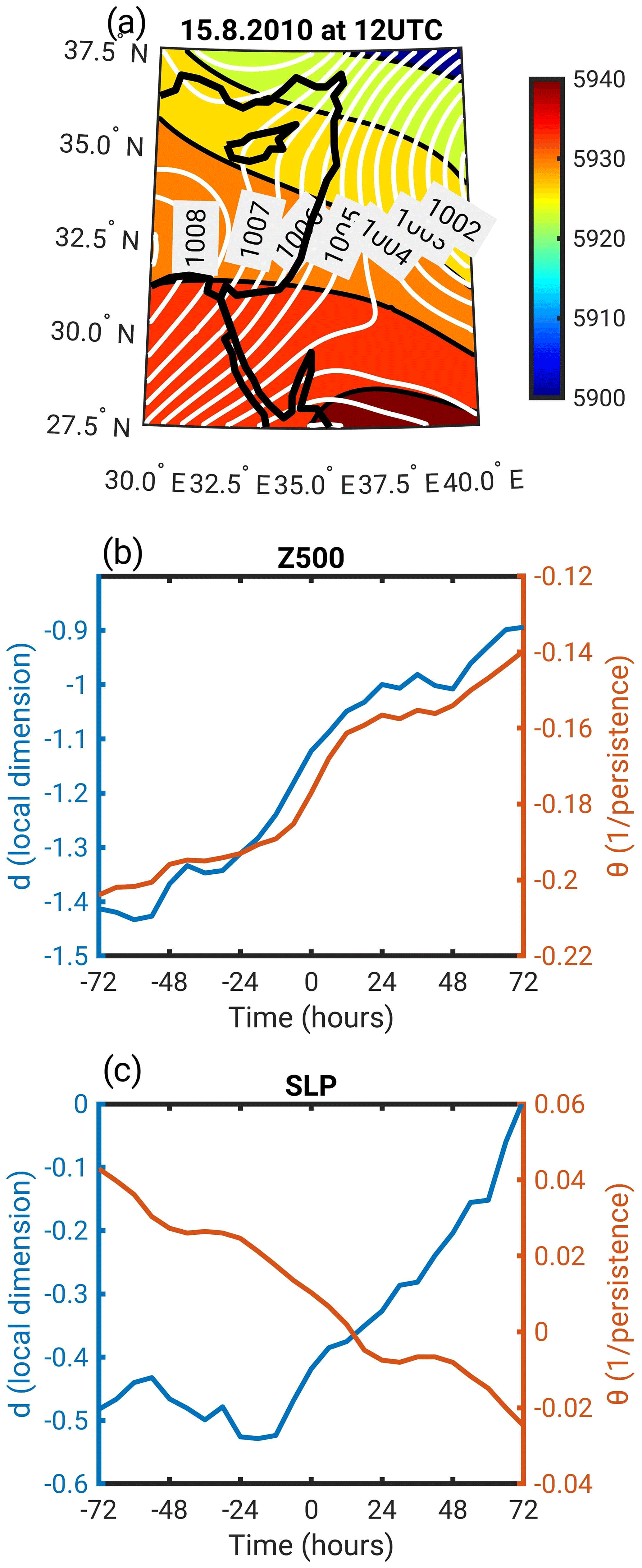
Figure 6A dynamical systems analysis for the mid-August 2010 heat wave. (a) SLP (white contours, in hPa) and Z500 (shading, in m) on 15 August 2010 at 12:00 UTC. The dynamical systems metrics' (d and θ) temporal evolution centered on 15 August 2010 at 12:00 UTC (0 h) computed on (b) Z500 and (c) SLP.
3.2 Analysis of the mid-August 2010 heat wave over the eastern Mediterranean
The mid-August 2010 heat wave over the eastern Mediterranean was a severe event, which lies in the upper 0.3 % of the CSI distribution. A detailed analysis of the heat wave highlights both similarities and differences with the climatology of the heat wave days (Sect. 3.1). The Z500 and SLP patterns for 15 August 2010 are comparable with the average configuration of a heat wave, but they show a stronger upper-level ridge and meridionally oriented isobars (cf. Figs. 6a and 1a). From a dynamical systems point of view, the 2010 heat wave was also an uncommon extreme, especially for the metrics computed on Z500. The dynamical systems metrics' anomalies computed on this field range between −0.9 and −1.4 for d and between −0.14 and −0.2 for θ (Fig. 6b). This situates the heat wave in the lower 10 % of the respective distributions (see also red dots in Fig. 3a). During its evolution, the event displays an increase in both d and θ computed on Z500 and a decrease (increase) in θ(d) computed on SLP (Fig. 6b, c). Whereas the Z500 d and θ evolution is roughly comparable to that identified for heat wave days (cf. Figs. 4a and 6b), the SLP d and θ evolutions show profound differences. This may simply reflect the larger spread in dynamical systems properties across the different heat waves for SLP than for Z500, which is likely to be partially modulated by interactions between the surface and the atmosphere. Naturally, these interactions predominantly affect the lowermost parts of the troposphere. We further hypothesize that differences between the single case and the climatology may be related to the relatively small day-to-day variations during summer over the eastern Mediterranean, which make it challenging to depict the exact onset of a heat wave. Indeed, when comparing the climatology of the temporal evolution of d and θ for Z500 (Fig. 4a) with the single case (Fig. 6b), it is relatively easy to see that there is an increase in both d and θ as the heat wave develops. On the other hand, when comparing the temporal evolution of d and θ for SLP (Figs. 4c with 6c), one can see that depicting the exact time that the heat wave starts is very important for comparison. In both Figures, d increases and θ decreases at some point in the chosen time window, but the timing of these trends is shifted between the climatology (Fig. 4c) and the single case (Fig. 6c).
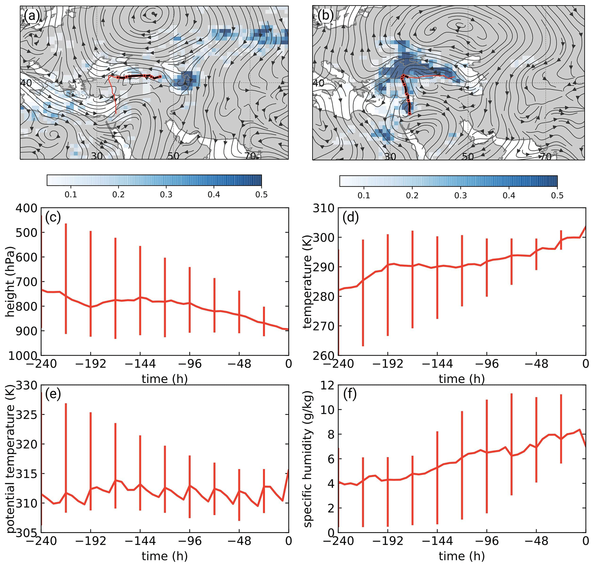
Figure 7Backward trajectory air parcel tracking for the mid-August 2010 heat wave initialized on 15 August 2010 at 12:00 UTC with (a) circles indicating days (from −10 to −6 d before 15 August 2010 at 12:00 UTC), gray shading indicating trajectory density 10 d before onset (number of trajectories per 1000 km2) and streamlines of 800 hPa wind (averaged between −10 and −6 d before 15 August 2010 at 12:00 UTC). Panel (b) is the same as panel (a) but for −5 to −1 d and a trajectory density of 5 d before onset. The median evolution of (c) height (hPa), (d) temperature (K), (e) potential temperature (K) and (f) specific humidity (g kg−1) of the tracked air parcels is also shown. The interquartile range is plotted for the physical properties of the air parcels. A value of 0 h corresponds to 15 August 2010 at 12:00 UTC.
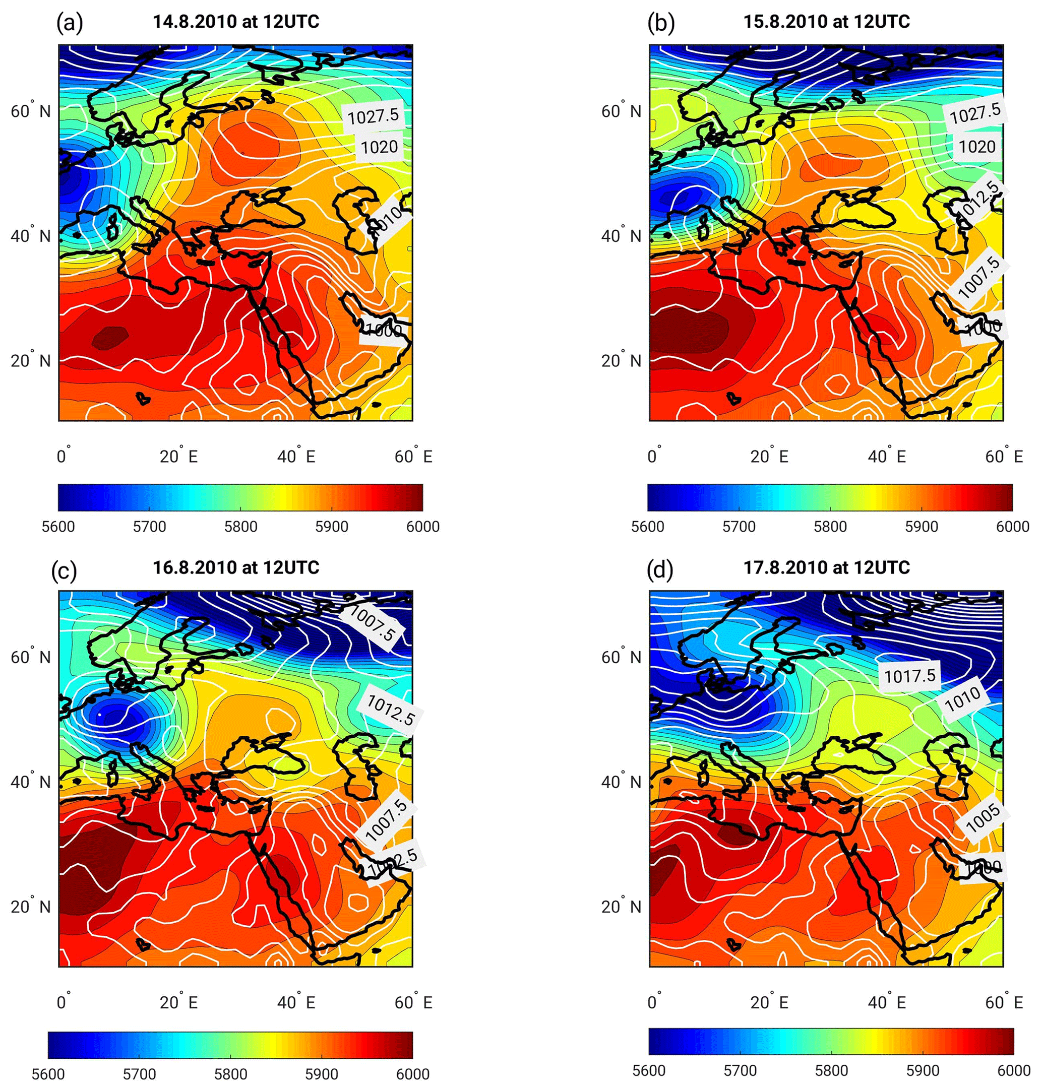
Figure 8The large-scale evolution of SLP (white contours, in hPa) and Z500 (shading, in m) for the mid-August 2010 heat wave: (a) 14 August 2010 at 12:00 UTC, (b) 15 August 2010 at 12:00 UTC, (c) 16 August 2010 at 12:00 UTC and (d) 17 August 2010 at 12:00 UTC.
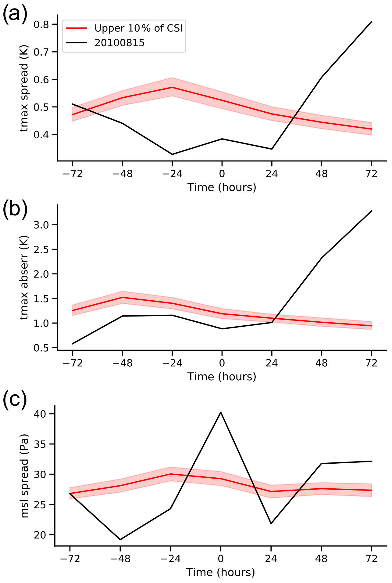
Figure 9Forecast spread and skill for the mid-August 2010 heat wave, centered (0 h) on 15 August 2010 at 12:00 UTC (black line). The mean temporal evolution of the ensemble model spread for Tmax (a), SLP (c) and the absolute error for Tmax (b) of forecasts with a lead time of 69 h, initialized at different time lags with respect to the event, computed every 24 h. The heat waves (upper 10 % of CSI – red lines) are displayed for reference. A 95 % bootstrap confidence interval for all heat waves is displayed (shading).
The 2010 heat wave was also uncommon in terms of the large-scale flow and Lagrangian trajectories (Fig. 7). Between −10 and −5 d prior to the event, the majority of air parcels were transported in an easterly flow on the southern flank of an anticyclone located over Russia. Thus, air parcels came from the Zagros Plateau of northern Iran, rather than from central Europe as in the climatology (cf. Figs. 7a, b and 2a). Indeed, Zaitchik et al. (2007) argued that the Zagros Plateau has a strong influence on extreme summertime heat waves over the eastern Mediterranean. Here we show that the anticyclonic wave breaking of the blocking regime over Russia, which interestingly is related to the decay phase of the Russian 2010 heat wave (Quandt et al., 2019), played an important role in transporting the warm air masses from northern Iran towards the eastern Mediterranean and Israel (Figs. 7a, b and 8). This is realized through the trough east of the blocking ridge centered over European Russia, which is tilted southwest–northeast and advected westward (Fig. 8b, c, d, Davini et al., 2012; Quandt et al., 2019). For the last 5 d prior to the heat wave (Fig. 7b), the parcel's trajectories more closely resemble the climatology of heat waves (Fig. 2a). Reflecting the different advection pathways, the initial potential temperature and temperature of the air parcels are about 2 and 7 K higher than the climatology of heat waves, respectively (cf. Figs. 7d, e and 2d, e). Accordingly, the hot air masses in the mid-August 2010 heat wave are transported to the eastern Mediterranean and undergo adiabatic heating, rather than being heated up locally. This is in line with the climatology discussed in Sect. 3.1 as well as heat waves in other parts of the world (e.g., Bieli et al., 2015; Quinting and Reeder, 2017; Zschenderlein et al., 2019).
Figure 9 shows the temporal evolution of the forecast spread and skill for the mid-August 2010 heat wave compared to the heat wave climatology. Throughout the lead-up and early phases of the event, the forecast displays a lower spread and error than for other heat waves. A large decrease in the practical predictability occurs as the event develops, i.e., an increase in the spread and decrease in the skill for maximum temperature (Fig. 9a, b). This mirrors the increase in d and θ computed on Z500 and for d computed on SLP (cf. Figs. 9a, b with Fig. 6b, c). Indeed, the decay phase of the Russian heat wave was characterized by low practical predictability (Matsueda, 2011), which may have influenced the predictability over the eastern Mediterranean. However, it should be noted that the spread computed on the maximum temperature for the mid-August 2010 heat wave does not correlate well with the spread computed on SLP (cf. Fig. 9a with c). Moreover, some striking differences are displayed between the ensemble forecast of this single event and the climatology of forecasts for heat waves. These discrepancies may be related to the fact that we are analyzing a single event, whose error may not reflect the practical predictability of the atmosphere even for a perfect ensemble (e.g., Whitaker and Lough, 1998; Buizza et al., 2005; Hopson 2014). The corresponding plots for forecast valid time (see Sect. 2.4) are provided in Fig. S4.
Heat waves are a major weather-related hazard, especially in an era of rapid climate change. We define heat waves over the eastern Mediterranean according to a state-of-the-art `climatic stress index' (CSI; Saaroni et al., 2017), developed specifically for the region's summer weather conditions. We use a combination of dynamical systems theory, numerical weather forecasts and air parcel back-trajectories to investigate the evolution and predictability characteristics of heat waves (high CSI) and cool days (low CSI) for the region.
The main conclusions are as follows: significant differences are found between heat waves and cool days from both a dynamical systems and numerical weather prediction perspectives. Heat waves show relatively low practical predictability (large model spread and low skill) in the ensemble reforecast dataset used here, in spite of the relatively stable flow characteristics (high intrinsic predictability) compared with the cool days. When considering Z500, the intrinsic predictability of heat waves over the eastern Mediterranean is highest, i.e., low local dimension (d) and high persistence (low θ), in the 24 h preceding the onset of the event and lowest in the decay phase of the event. Indeed, Lucarini and Gritsun (2020) recently argued that atmospheric blocking over the Atlantic also displays such characteristics. The persistent upper-level ridge that characterizes the heat waves may explain the high intrinsic predictability during the onset phase. The dynamical systems metrics computed on SLP show a different temporal evolution to their Z500 counterparts, emphasizing the different characteristics of the atmospheric flow at the different vertical levels. Specifically, there is a very large spread across different heat wave events. We argue that this may be associated with the delicate interplay between the subtropical high and the Persian trough at surface levels (Alpert et al., 1990), which can lead to a range of different SLP configurations all leading to a heat wave. This may further be reasonably attributed to the interactions between the land and/or sea surface and the atmosphere, which mainly influence the lower parts of the troposphere. However, it is important to note that in many – albeit certainly not all – cases these interactions influence the atmosphere at timescales longer than those we consider in our analysis (e.g., Entin et al., 2000), and they can act as a seasonal-scale preconditioning to extremely high summer temperatures (Zampieri et al., 2009; Zittis et al., 2014).
Based on the Lagrangian air parcel analysis, we conclude that the physical processes governing eastern Mediterranean summer heat waves relate to adiabatic descent of the air parcels over the region rather than diabatic heating, in agreement with previous findings (e.g., Harpaz et al., 2014). In other words, the air parcels are transported horizontally and vertically towards the eastern Mediterranean with the governing westerlies rather than heated up locally over consecutive days. We further conclude that the origin of the air parcels over land in the days before the onset of a heat wave plays an important part in its generation.
A detailed analysis of the record-breaking mid-August 2010 heat wave provides further insights in this respect by underscoring how the parcels, which contributed to the heat wave, were warmer than those of the climatology of heat waves as early as 10 d prior to the event. Interestingly, the onset of the heat wave over the eastern Mediterranean was related to the decay phase of the Russian heat wave (Quandt et al., 2019), and we conclude that the anticyclonic Rossby wave breaking over Russia contributed to the onset of the eastern Mediterranean heat wave. The 2010 heat wave showed both differences and similarities to other heat waves, highlighting the range of possible atmospheric and dynamical developments leading to high CSI values. This is compounded by the general difficulty of analyzing the life cycle of heat waves, as there is little agreement as to what exactly a heat wave is and when it starts and ends (Shaby et al., 2016).
We conclude that the instantaneous dynamical systems metrics of local dimension (d) and persistence (θ−1) provide complementary information on extreme summer heat waves compared with the conventional analysis of numerical weather forecasts. The discrepancy between the practical and the intrinsic predictability of the heat waves reflects this complementarity. For example, we interpret a very persistent system as being intrinsically highly predictable, yet the numerical forecasts we analyze display larger spread and error for the more persistent atmospheric configurations. In this respect, having an a priori measure of the persistence of an atmospheric configuration from dynamical systems can be a useful complement to the numerical forecast. Specifically, the practical predictability relies on the performance of a numerical forecast model. As such, it blends model and data assimilation biases with the intrinsic characteristics of the atmospheric flow. Moreover, even a perfect ensemble may not provide a good spread–skill relationship (Hopson, 2014). That is, even a perfect ensemble may have a spread that does not always reflect the actual forecast error (Whitaker and Lough, 1998; Buizza, 1997). In the specific case of the heat waves that we analyze here, the spread and skill were well correlated for maximum temperature, but this is not a universal rule. For example, the mid-August 2003 heat wave had a very low spread (Tmax spread = 0.2 K; cf. Fig. 5b) and an above average error (Tmax absolute error = 1.1 K; cf. Fig. 5d). However, both d and θ computed on Z500 display a strong increase (d = −1.7 to 0.3, to 0.1 over the considered time window, not shown; cf. Figs. 4a and 6b), pointing to a decrease in intrinsic predictability. In such cases, local dimension (d) and/or persistence (θ−1) trends that seem to contradict a low ensemble spread may serve as a warning of a potentially poor spread–skill relationship.
As a caveat, the comparison of the practical and intrinsic predictability still carries some interpretation challenges. Although the differences between the two can be partly ascribed to the different characteristics of the two measures, they may also be subject to the shortcomings of the GEFS ensemble data. In particular, the spread of the GEFS ensemble data, as most NWP ensemble forecasts, does not always reflect the practical predictability of the atmospheric flow (e.g., Whitaker and Lough, 1998). Moreover, our interpretation of the dynamical systems metrics may also be imperfect. Indeed, the metrics provide local information in phase space, whereas the spread and error of an ensemble forecast presumably reflect the longer-term evolution of the atmospheric flow. Similar interpretation challenges for the practical versus intrinsic predictability have emerged when studying cold spells over the eastern Mediterranean (Hochman et al., 2020a).
Notwithstanding these ongoing challenges, we believe that the novel view presented here, which leverages a dynamical systems approach for diagnosing extreme weather events, outlines an important avenue of research. We trust that it may be successfully applied to other regions and weather extremes in the future.
The code for computing the dynamical systems metrics is publicly available at https://www.lsce.ipsl.fr/Pisp/davide.faranda/ (Laboratoire des Sciences du Climat et de l'Environment, 2021), and code for computing backward trajectories is publicly available at https://iacweb.ethz.ch/staff/sprenger/lagranto/ (ETH Zürich, 2021).
The paper and/or the Supplement contain or provide instructions to access all of the data needed to evaluate the conclusions drawn in the paper. Additional data are available from the corresponding author upon request.
The supplement related to this article is available online at: https://doi.org/10.5194/esd-12-133-2021-supplement.
All authors contributed to the conceptual development of the study. AH and GM analyzed the data from a dynamical systems perspective. SS analyzed the forecast model data. JQ computed the air parcel backward trajectories. AH drafted the first version of the paper. All authors contributed through discussions and revisions.
The authors declare that they have no conflict of interest.
We would like to thank Yitzhak Yosef, head of the Climate Research department at the Israeli Meteorological Service (IMS), for providing homogeneous high-quality continuous station data over Israel. We are also grateful to Noam Halfon of the IMS for providing averaged summer temperatures computed from the IMS Climatic Atlas. We thank the National Centers for Environmental Prediction/National Center for Atmospheric Research for the Reanalysis data and the Global Ensemble Forecast System reforecasts. We are grateful to Heini Wernli and the Atmospheric Dynamics group at ETH Zurich for sharing the ERA-Interim data. This paper is a contribution to the Hydrological cycle in the Mediterranean eXperiment (HyMeX) community.
Assaf Hochman is funded by the German Helmholtz Association (ATMO program). The contribution of Julian Quinting was funded by the Helmholtz Association (grant no. VH-NG-1243). Joaquim G. Pinto received funding from the AXA Research Fund. Gabriele Messori was partly funded
by the Swedish Research Council Vetenskapsrådet (grant no. 2016-03724).
The article processing charges for this open-access
publication were covered by a Research
Centre of the Helmholtz Association.
This paper was edited by Sagnik Dey and reviewed by two anonymous referees.
Aguilar, E., Auer, I., Brunet, M., Peterson, T. C., and Wieringa, J.: Guide-lines on climate metadata and homogenization, WCDMP-No. 53, WMO-TDNo. 1186, World Meteorological Organization, Geneva, Switzerland, 2003.
Alpert, P., Abramsky, R., and Neeman, B. U.: The prevailing summer synoptic system in Israel – Subtropical High, not Persian Trough, Israel J. Earth Sci., 39, 93–102, 1990.
Alpert, P., Osetinsky, I., Ziv, B., and Shafir, H.: Semi-objective classification for daily synoptic systems: Application to the Eastern Mediterranean climate change, Int. J. Climatol., 24, 1001–1011, https://doi.org/10.1002/joc.1036, 2004a.
Alpert, P., Osetinsky, I., Ziv, B., and Shafir, H.: A new seasons' definition based on the classified daily synoptic systems, an example for the Eastern Mediterranean, Int. J. Climatol., 24, 1013–1021, https://doi.org/10.1002/joc.1037, 2004b.
Baldi, M., Dalu, G., Marrachi, G., Pasqui, M., and Cesarone, F.: Heat waves in the Mediterranean: A local feature or a larger-scale effect?, Int. J. Climatol., 26, 1477–1488, https://doi.org/10.1002/joc.1389, 2006.
Ballester, J., Robine, J. M., Herrmann, F. R., and Rodó, X.: Effect of the Great Recession on regional mortality trends in Europe, Nat. Commun., 10, 679, https://doi.org/10.1038/s41467-019-08539-w, 2019.
Barcikowska, M. J., Kapnick, S. B., Krishnamurty, L., Russo, S., Cherchi, A., and Folland, C. K.: Changes in the future summer Mediterranean climate: contribution of teleconnections and local factors, Earth Syst. Dynam., 11, 161–181, https://doi.org/10.5194/esd-11-161-2020, 2020.
Barriopedro, D., Fischer, E. M., Luterbacher, J., Trigo, R. M., and García-Herrera, R.: The hot summer of 2010: redrawing the temperature record map of Europe, Science, 332, 220–224, https://doi.org/10.1126/science.1201224, 2011.
Battisti, D. S. and Naylor, R. L.: Historical warnings of future food insecurity with unprecedented seasonal heat, Science, 323, 240–244, https://doi.org/10.1126/science.1164363, 2009.
Bennett, J. E., Blangiardo, M., Fecht, D., Elliott, P., and Ezzati, M.: Vulnerability to the mortality effects of warm temperature in the districts of England and wales, Nat. Clim. Change, 4, 269–273, https://doi.org/10.1038/nclimate2123, 2014.
Bieli, M., Pfahl, S., and Wernli, H.: A Lagrangian investigation of hot and cold temperature extremes in Europe, Q. J. Roy. Meteor. Soc., 141, 98–108, https://doi.org/10.1002/qj.2339, 2015.
Bitan, A. and Saaroni, H.: The horizontal and vertical extension of the Persian Gulf trough, Int. J. Climatol., 12, 733–747, https://doi.org/10.1002/joc.3370120706, 1992.
Black, E., Blackburn, M., Harrison, R. G., Hoskins, B. J., and Methven, J.: Factors contributing to the summer 2003 European heatwave, Weather, 59, 217–223, https://doi.org/10.1256/wea.74.04, 2004.
Buizza, R.: Potential forecast skill of ensemble prediction and spread and skill distributions of the ECMWF ensemble prediction system, Mon. Weather Rev., 125, 99-119, 1997.
Buizza, R., Houtekamer, P. L., Pellerin, G., Toth, Z., Zhu, Y., and Wei, M.: A Comparison of the ECMWF, MSC, and NCEP Global Ensemble Prediction Systems, Mon. Weather Rev., 133, 1076–1097, 2005.
Buschow, S. and Friederichs, P.: Local dimension and recurrent circulation patterns in long-term climate simulations, Chaos, 28, 083124, https://doi.org/10.1063/1.5031094, 2018.
Brunetti, M., Kasparian, J., and Vérard, C.: Co-existing climate attractors in a coupled aqua-planet, Clim. Dynam., 53, 6293–6308, https://doi.org/10.1007/s00382-019-04926-7, 2019.
Caby, T., Faranda, D., Vaienti, S., and Yiou, P.: Extreme value distributions of observation recurrences, arXiv [preprint], Nonlinearity, 34, 118, https://doi.org/10.1088/1361-6544/abaff1, 2020.
Caldeira, M. C., Lecomte, X., David, T. S., Pinto, J. G., Bugalho, M. N., and Werner, C.: Synergy of extreme drought and plant invasion reduce ecosystem functioning and resilience, Sci. Rep.-UK, 5, 15110, https://doi.org/10.1038/srep15110, 2015.
Davini, P., Cagnazzo, C., Gualdi, S., and Navarra, A.: Bidimensional diagnostics, variability, and trends of northern hemisphere 2015 blocking, J. Climate, 25, 6496–6509, https://doi.org/10.1175/JCLI-D-12-00032.1, 2012.
Dayan, U., Tubi, A., and Levy, I.: On the importance of synoptic classification methods with respect to environmental phenomena, Int. J. Climatol., 32, 681–694, https://doi.org/10.1002/joc.2297, 2012.
Dee, D. P., Uppala, S. M., Simmons, A. J., Berrisford, P., Poli, P., Kobayashi, S., Andrae, U., Balmaseda, M. A., Balsamo, G., Bauer, P., Bechtold, P., Beljaars, A. C. M., Van de Berg, L., Bidlot, J., Bormann, N., Delsol, C., Dragani, R., Fuentes, M., Geer, A. J., Haimberger, L., Healy, S. B., Hersbach, H., Hólm, E. V., Isaksen, L., Kållberg, P., Köhler, M., Matricardi, M., McNally, A. P., Monge-Sanz, B. M., Morcrette, J. J., Park, B. K., Peubey, C., De Rosnay, P., Tavolato, C., Thépaut, J. N., and Vitart, F.: The ERA-Interim reanalysis: configuration and performance of the data assimilation system, Q. J. Roy. Meteor. Soc., 137, 553–597, https://doi.org/10.1002/qj.828, 2011.
De Luca, P., Messori, G., Pons, F. M. E., and Faranda, D.: Dynamical systems theory sheds new light on compound climate extremes in Europe and Eastern North America, Q. J. Roy. Meteor. Soc., 146, 1636–1650, https://doi.org/10.1002/qj.3757, 2020a.
De Luca, P., Messori, G., Faranda, D., Ward, P. J., and Coumou, D.: Compound warm–dry and cold–wet events over the Mediterranean, Earth Syst. Dynam., 11, 793–805, https://doi.org/10.5194/esd-11-793-2020, 2020b.
Deryng, D., Conway, D., Ramankutty, N., Price, J., and Warren, R.: Global crop yield response to extreme heat stress under multiple climate change futures, Environ. Res. Lett., 9, 034011, https://doi.org/10.1088/1748-9326/9/3/034011, 2014.
Dirmeyer, P. A., Halder, S., and, Bombardi, R.: On the harvest of predictability from land states in a global forecast model, J. Geophys. Res.-Atmos., 123, 111–127, https://doi.org/10.1029/2018JD029103, 2018.
Easterling, D. R., Meehl, G. A., Parmesan, C., Changnon, S. A., Karl, T. R., and Mearns, L. O.: Climate extremes: Observations, modelling and impacts, Science, 289, 2068–2074, https://doi.org/10.1126/science.289.5487.2068, 2000.
Entin, J. K., Robock, A., Vinnikov, K. Y., Hollinger, S. E., Liu, S., and Namkhai, A.: Temporal and spatial scales of observed soil moisture variations in the extra tropics, J. Geophys. Res., 105, 11865–11877, https://doi.org/10.1029/2000JD900051, 2000.
Epstein, Y. and Moran, D. S.: Thermal comfort and the Heat Stress Indices, Industrial Health, 44, 388–398, https://doi.org/10.2486/indhealth.44.388, 2006.
ETH Zürich: LAGRANTO, available at: https://iacweb.ethz.ch/staff/sprenger/lagranto/, last access: 29 January 2021.
Faranda, D., Messori, G., and Yiou, P.: Dynamical proxies of North Atlantic predictability and extremes, Sci. Rep.-UK, 7, 41278, https://doi.org/10.1038/srep41278, 2017a.
Faranda, D., Messori, G., Alvarez-Castro, M. C., and Yiou, P.: Dynamical properties and extremes of Northern Hemisphere climate fields over the past 60 years, Nonlin. Processes Geophys., 24, 713–725, https://doi.org/10.5194/npg-24-713-2017, 2017b.
Faranda, D., Messori, G., and Vannistem, S.: Attractor dimension of time-averaged climate observables: insights from a low-order ocean-atmosphere model, Tellus A, 71, 1554413, https://doi.org/10.1080/16000870.2018.1554413, 2019a.
Faranda, D., Alvarez-Castro, M. C., Messori, G., Rodrigues, D., and Yiou, P.: The hammam effect or how a warm ocean enhances large scale atmospheric predictability, Nat. Commun., 10, 1316, https://doi.org/10.1038/s41467-019-09305-8, 2019b.
Faranda, D., Sato, Y., Messori, G., Moloney, N. R., and Yiou, P.: Minimal dynamical systems model of the Northern Hemisphere jet stream via embedding of climate data, Earth Syst. Dynam., 10, 555–567, https://doi.org/10.5194/esd-10-555-2019, 2019c.
Faranda, D., Messori, G., and Yiou, P.: Diagnosing concurrent drivers of weather extremes: application to warm and cold days in North America, Clim. Dynam., 54, 2187–2201, https://doi.org/10.1007/s00382-019-05106-3, 2020.
Ferranti, L., Corti, S., and Janousek, M.: Flow-dependent verification of the ECMWF ensemble over the Euro-Atlantic sector, Q. J. Roy. Meteor. Soc., 141, 916–924, https://doi.org/10.1002/qj.2411, 2015.
Fischer, E. M. and Schär, C.: Consistent geographical patterns of changes in high-impact European heatwaves, Nat. Geosci., 3, 398–403, https://doi.org/10.1038/ngeo866, 2010.
Freitas, A. C. M., Freitas, J. M., and Todd, M.: Hitting time statistics and extreme value theory, Probab. Theory Rel., 147, 675–710, https://doi.org/10.1007/s00440-009-0221-y, 2010.
Giorgi, F.: Climate change hot spots, Geophys. Res. Lett., 33, L08707, https://doi.org/10.1029/2006gl025734, 2006.
Grumm, R. H.: The Central European and Russian Heat Event of July–August 2010, B. Am. Meteorol. Soc., 92, 1285–1296, https://doi.org/10.1175/2011bams3174.1, 2011.
Hamill, T. M., Bates, G. T., Whitaker, J. S., Murray, D. R., Fiorino, M., Galarneau, T. J., Zhu, Y., and Lapenta, W.: NOAA's Second-Generation Global Medium-Range Ensemble Reforecast Dataset, B. Am. Meteorol. Soc., 94, 1553–1565, https://doi.org/10.1175/bams-d-12-00014.1, 2013.
Harpaz, T., Ziv, B., Saaroni, H., and Beja, E.: Extreme summer temperatures in the East Mediterranean – dynamical analysis, Int. J. Climatol., 34, 849–862, https://doi.org/10.1002/joc.3727, 2014.
Hochman, A., Mercogliano, P., Alpert, P., Saaroni, H., and Bucchignani, E.: High-resolution projection of climate change and extremity over Israel using COSMO-CLM, Int. J. Climatol., 38, 5095–5106, https://doi.org/10.1002/joc.5714, 2018a.
Hochman, A., Alpert, P., Harpaz, T., Saaroni, H., and Messori, G.: A new dynamical systems perspective on atmospheric predictability: eastern Mediterranean weather regimes as a case study, Sci. Adv., 6, 1–10, https://doi.org/10.1126/sciadv.aau0936, 2019.
Hochman, A., Scher, S., Quinting, J., Pinto, J. G., and Messori, G.: Dynamics and predictability of cold Spells over the Eastern Mediterranean, Clim. Dynam., https://doi.org/10.1007/s00382-020-05465-2, 2020a.
Hochman, A., Alpert, P., Kunin, P., Rostkier-Edelstein, D., Harpaz, T., Saaroni, H., and Messori, G.: The dynamics of cyclones in the 21st century; the eastern Mediterranean as an example, Clim. Dynam., 54, 561–574, https://doi.org/10.1007/s00382-019-05017-3, 2020b.
Hohenegger, C., Lüthi, D., and Schär, C.: Predictability mysteries in cloud-resolving Models, Mon. Weather Rev., 134, 2095–2107, https://doi.org/10.1175/mwr3176.1, 2006.
Holton, J. R.: An introduction to dynamic meteorology, Elsevier, London, UK, 2004.
Hopson, T. M.: Assessing the ensemble spread-error relationship, Mon. Weather Rev., 142, 1125–1142, https://doi.org/10.1175/MWR-D-12-00111.1, 2014.
IPCC: Managing the Risks of Extreme Events and Disasters to Advance Climate Change Adaptation, edited by: Field, C. B., Barros, V., Stocker, T. F., Qin, D., Dokken, D. J., Ebi, K. L., Mastrandrea, M. D., Mach, K. J., Plattner, G. K., Allen, S. K., Tignor, M., and Midgley, P. M., Cambridge University Press, The Edinburgh Building, Shaftesbury Road, Cambridge CB2 8RU ENGLAND, 582 pp., https://doi.org/10.1017/cbo9781139177245, 2012.
Kalnay, E., Kanamitsu, M., Kistler, R., Collins, W., Deaven, D., Gandin, L., Iredell, M., Saha, S., White, G., Woollen, J., Zhu, Y., Chelliah, M., Ebisuzaki, W., Higgins, W., Janowiak, J., Mo, K. C., Ropelewski, C., Wang, J., Leetmaa, A., Reynolds, R., Jenne, R., and Joseph, D.: The NCEP/NCAR 40-Year reanalysis project, B. Am. Meteorol. Soc., 77, 437–471, 1996.
Katsafados, P., Papadopoulos, A., Varlas, G., Papadopoulou, E., and Mavromatidis, E.: Seasonal predictability of the 2010 Russian heat wave, Nat. Hazards Earth Syst. Sci., 14, 1531–1542, https://doi.org/10.5194/nhess-14-1531-2014, 2014.
Keune, J., Ohlwein, C., and Hense, A.: Multivariate probabilistic analysis and predictability of medium-range ensemble weather forecasts, Mon. Weather Rev., 142, 4074–4090, https://doi.org/10.1175/mwr-d-14-00015.1, 2014.
Koster, R. D., Mahanama, S. P. P., Yamada, T. J., Balsamo, G., Berg, A. A., Boisserie, M., Dirmeyer, P. A., Doblas-Reyes, F. J., Drewitt, G., Gordon, C. T., Guo, Z., Jeong, J. H., Lawrence, D. M., Lee, W. S., Li, Z., Luo, L., Malyshev, S., Merryfield, W. J., Seneviratne, S. I., Stanelle, T., van den Hurk, B. J. J. M., Vitart, F., ad Wood, E. F.: Contribution of land surface initialization to sub-seasonal forecast skill: First results from a multi-model experiment, Geophys. Res. Lett., 37, 1–6, https://doi.org/10.1029/2009GL041677, 2010.
Kuglitsch, F., Toreti, A., Xoplaki, E., Della-Martta, P., Zerefos, C. S., Türkeş, M., and Luterbacher, J.: Heat wave changes in the Eastern Mediterranean since 1960, Geophys. Res. Lett., 37, L04802, https://doi.org/10.1029/2009gl041841, 2010.
Kunin, P., Alpert, P., and Rostkier-Edelstein, D.: Investigation of sea-breeze/foehn in the Dead-Sea valley employing high-resolution WRF and observations, Atmos. Res., 229, 240–254, https://doi.org/10.1016/j.atmosres.2019.06.012, 2019.
Kushnir, Y., Dayan, U., Ziv, B., Morin, E., and Enzel, Y.: Climate of the Levant: phenomena and mechanisms, in: Quaternary of the Levant: environments, climate change, and humans, edited by: Enzel, Y. and Ofer, B.-Y., Cambridge University Press, Cambridge, UK, 31–44, 2017.
Laboratoire des Sciences du Climat et de l'Environment: Davide Faranda, available at: https://www.lsce.ipsl.fr/Pisp/davide.faranda/, last access: 29 January 2021.
Lelieveld, J., Proestos, Y., Hadjinicolaou, P., Tanarhte, M., Tyrlis, E., and Zittis, G.: Strongly increasing heat extremes in the Middle East and North Africa (MENA) in the 21st century, Climatic Change, 137, 245–260, https://doi.org/10.1007/s10584-016-1665-6, 2016.
Loken, E. D., Clark, J. C., Xue, M., and Kong, F.: Spread and skill in mixed and single physics convection allowing ensembles, Weather Forecast., 34, 305–330, https://doi.org/10.1175/waf-d-18-0078.1, 2019.
Lorenz, E. N.: Deterministic non-periodic flow, J. Atmos. Sci., 20, 130–141, 1963.
Lorenz, E. N.: Atmospheric predictability as revealed by naturally occurring analogues, J. Atmos. Sci., 26, 636–646, 1969.
Lucarini, V. and Gritsun, A.: A new mathematical framework for atmospheric blocking events, Clim. Dynam., 54, 575–598, https://doi.org/10.1007/s00382-019-05018-2, 2020.
Lucarini, V., Faranda, D., and Wouters, J.: Universal behavior of extreme value statistics for selected observables of dynamical systems, J. Stat. Phys., 147, 63–73, https://doi.org/10.1007/s10955-012-0468-z, 2012.
Lucarini, V., Faranda, D., Freitas, A. C. M., Freitas, J. M., Holland, M., Kuna, T., Nicol, M., Todd, M., and Vaienti, S.: Extremes and recurrence in dynamical systems, in: Pure and Applied Mathematics, edited by: Lucarini, V., Faranda, D., Freitas, A. C. G. M. M. D., Freitas, J. M. M. D., Holland, M., Kuna, T., Nicol, M., Todd, M., and Vaienti, S.: Extreme Value Theory for Selected Dynamical Systems, Wiley, Hoboken, NJ, USA, 126–172, https://doi.org/10.1002/9781118632321.ch6, 2016.
Matsueda, M.: Predictability of Euro-Russian blocking in summer of 2010, Geophys. Res. Lett., 38, L06801, https://doi.org/10.1029/2010gl046557, 2011.
Matsueda, M. and Palmer, T. N.: Estimates of flow-dependent predictability of wintertime Euro-Atlantic weather regimes in medium-range forecasts, Q. J. Roy. Meteor. Soc., 144, 1012–1027, https://doi.org/10.1002/qj.3265, 2018.
Meehl, G. A. and Tebaldi, C.: More intense, more frequent, and longer lasting heatwaves in the 21st century, Science, 305, 994–997, https://doi.org/10.1126/science.1098704, 2004.
Melhauser, C. and Zhang, F.: Practical and intrinsic predictability of severe and convective weather at the mesoscales, J. Atmos. Sci., 69, 3350–3371, https://doi.org/10.1175/JAS-D-11-0315.1, 2012.
Messori, G., Caballero, R., and Faranda, D.: A dynamical systems approach to studying midlatitude weather extremes, Geophys. Res. Lett., 44, 3346–3354, https://doi.org/10.1002/2017gl072879, 2017.
Moloney, N. R., Faranda, D., and Sato, Y.: An overview of the extremal index, Chaos, Interdisciplinary Journal of Nonlinear Science, 29, 022101, https://doi.org/10.1063/1.5079656, 2019.
Peterson, T. C., Heim Jr., R. R., Hirsch, R., Kaiser, D. P., Brooks, H., Diffenbaugh, N. S., Dole, R. M., Giovannettone, J. P., Guirguis, K., Karl, T. R., Katz, R. W., Kunkel, K., Lettenmaier, D., McCabe, G. J., Paciorek, C. J., Ryberg, K. R., Schubert, S., Silva, V. B. S., Stewart, B. C., Vecchia, A. V., Villarini, G., Vose, R. S., Walsh, J., Wehner, M., Wolock, D., Wolter, K., Woodhouse, C. A., and Wuebbles, D.: Monitoring and understanding changes in heat waves, cold waves, floods and droughts in the United States: State of knowledge, B. Am. Meteorol. Soc., 94, 821–834, https://doi.org/10.1175/bams-d-12-00066.1, 2013.
Pons, F. M. E., Messori, G., Alvarez-Castro, M. C., and Faranda, D.: Sampling hyperspheres via extreme value theory: implications for measuring attractor dimensions, J. Stat. Phys., 179, 1698–1717, https://doi.org/10.1007/s10955-020-02573-5, 2020.
Quandt, L. A., Keller, J. H., Martius, O., and Jones, S. C.: Forecast variability of the blocking system over Russia in summer 2010 and its impact on surface conditions, Weather Forecast., 32, 61–82, https://doi.org/10.1175/WAF-D-16-0065.1, 2017.
Quandt, L. A., Keller, J. H., Martius, O., Pinto, J. G., and Jones, S. C.: Ensemble sensitivity analysis of the blocking system over Russia in summer 2010, Mon. Weather Rev., 147, 657–675, https://doi.org/10.1175/mwr-d-18-0252.1, 2019.
Quinting, J. F. and Reeder, M. J.: Southeastern Australian heat waves from a trajectory viewpoint, Mon. Weather Rev., 145, 4109–4125, https://doi.org/10.1175/MWR-D-17-0165.1, 2017.
Quinting, J. F., Parker, T., and Reeder, M. J.: Two synoptic routes to subtropical heat waves as illustrated in the Brisbane region of Australia, Geophys. Res. Lett., 45, 10700– 10708, https://doi.org/10.1029/2018GL079261, 2018.
Rodrigues, D., Alvarez-Castro, M. C., Messori, G., Yiou, P., Robin, Y., and Faranda, D.: Dynamical properties of the North Atlantic atmospheric circulation in the Past 150 Years in CMIP5 Models and the 20CRv2c Reanalysis, J. Climate, 31, 6097–6111, https://doi.org/10.1175/jcli-d-17-0176.1, 2018.
Rodwell, M. J. and Hoskins, B.: Monsoons and the dynamic of deserts, Q. J. Roy. Meteorol. Soc., 122, 1385–1404, https://doi.org/10.1002/qj.49712253408, 1996.
Russo, S., Dosio, A., Graversen, R. G., Sillmann, J., Carrao, H., Dunbar, M. B., and Vogt, J. V.: Magnitude of extreme heatwaves in present climate and their projection in a warming world, J. Geophys. Res.-Atmos., 119, 1–13, https://doi.org/10.1002/2014jd022098, 2014.
Saaroni, H. and Ziv, B.: Summer rain episodes in a Mediterranean climate – the case of Israel: climatological-dynamical analysis, Int. J. Climatol., 20, 191–209, 2000.
Saaroni, H., Savir, A., and Ziv, B.: Synoptic classification of the summer season for the Levant using an “environment to climate” approach, Int. J. Climatol., 37, 4684–4699, https://doi.org/10.1002/joc.5116, 2017.
Santos, J. A., Pfahl, S., Pinto, J. G., and Wernli, H.: Mechanisms underlying temperature extremes in Iberia: a Lagrangian perspective, Tellus A, 67, 26032, https://doi.org/10.3402/tellusa.v67.26032, 2015.
Scher, S. and Messori, G.: Predicting weather forecast uncertainty with machine learning, Q. J. Roy. Meteor. Soc., 144, 2830–2841, https://doi.org/10.1002/qj.3410, 2018.
Schneidereit, A., Schubert, S., Vargin, P., Lunkeit, F., Zhu, X., Peters, D. H. W., and Fraedrich, K.: Large-scale flow and the long-lasting blocking high over Russia: Summer 2010, Mon. Weather Rev., 140, 2967–2981, https://doi.org/10.1175/mwr-d-11-00249.1, 2012.
Seneviratne, S. I., Nicholls, N., Easterling, D., Goodess, C. M., Kanae, S., Kossin, J., Luo, Y., Marengo, J., McInnes, K., Rahimi, M., Reichstein, M., Sorteberg, A., Vera, C., and Zhang, X.: Changes in climate extremes and their impacts on the natural physical environment, in: Managing the risks of extreme events and disasters to advance climate change adaptation, edited by: Field, C. B., Barros, V., Stocker, T. F., Qin, D., Dokken, D. J., Ebi, K. L., Mastrandrea, M. D., Mach, K. J., Plattner, G.-K., Allen, S. K., Tignor, M., and Midgley, P. M., Cambridge University Press, Cambridge, UK, 109–230, 2012.
Shaby, B. A., Reich, B. J., Cooley, D., and Kaufman, C. G.: A Markov-Switching model for heat waves, Ann. Appl. Stat., 10, 74–93, https://doi.org/10.1214/15-aoas873, 2016.
Siebert, S. and Ewert, F.: Future crop production threatened by extreme heat, Environ. Res. Lett., 9, 041001, https://doi.org/10.1088/1748-9326/9/4/041001, 2014.
Sprenger, M. and Wernli, H.: The LAGRANTO Lagrangian analysis tool – version 2.0, Geosci. Model Dev., 8, 2569–2586, https://doi.org/10.5194/gmd-8-2569-2015, 2015.
Stott, P. A., Stone, D. A., and Allen, M. R.: Human contribution to the European heatwave of 2003, Nature, 432, 610–614, https://doi.org/10.1038/nature03089, 2004.
Süveges, M.: Likelihood estimation of the extremal index, Extremes, 10, 41–55, https://doi.org/10.1007/s10687-007-0034-2, 2007.
Tyrlis, E. and Lelieveld, J.: Climatology and dynamics of the summer Etesian winds over the Eastern Mediterranean, J. Atmos. Sci., 70, 3374–3396, https://doi.org/10.1175/JAS-D-13-035.1, 2013.
Uzan, L., Egert, S., and Alpert, P.: Ceilometer evaluation of the eastern Mediterranean summer boundary layer height – first study of two Israeli sites, Atmos. Meas. Tech., 9, 4387–4398, https://doi.org/10.5194/amt-9-4387-2016, 2016.
Uzan, L., Egert, S., Khain, P., Levi, Y., Vadislavsky, E., and Alpert, P.: Ceilometers as planetary boundary layer height detectors and a corrective tool for COSMO and IFS models, Atmos. Chem. Phys., 20, 12177–12192, https://doi.org/10.5194/acp-20-12177-2020, 2020.
Wernli, H. and Davies, H. C.: A lagrangian-based analysis of extratropical cyclones. I: The method and some applications, Q. J. Roy. Meteor. Soc., 123, 467–489, https://doi.org/10.1002/qj.49712353811, 1997.
Whitaker, J. S. and Loughe, A. F.: The relationship between ensemble spread and ensemble mean skill, Mon. Weather Rev., 126, 3292–3302, https://doi.org/10.1175/1520-0493(1998)126<3292:TRBESA>2.0.CO;2, 1998.
Williams, C. A.: Heat and drought extremes likely to stress ecosystem productivity equally or more in a warmer, CO2 rich future, Environ. Res. Lett., 9, 101002, https://doi.org/10.1088/1748-9326/9/10/101002, 2014.
Yarnal, B.: Synoptic climatology in environmental analysis, Belhaven Press, London, UK, https://doi.org/10.1016/0160-4120(93)90293-q, 1993.
Yarnal, B., Comrie, A. C., Frakes, B., and Brown, D. P.: Developments and prospects in synoptic climatology – Review, Int. J. Climatol., 21, 1923–1950, https://doi.org/10.1002/joc.675, 2001.
Yosef, Y., Aguilar, E., and Alpert, P.: Detecting and adjusting artificial biases in long-term temperature records in Israel, Int. J. Climatol., 38, 3273–3289, https://doi.org/10.1002/joc.5500, 2018.
Zaitchik, B. F., Evans, J. P., and Smith, R. B.: Regional impact of an elevated heat source: The Zagros Plateau of Iran, J. Climate, 20, 4133–4166, https://doi.org/10.1175/jcli4248.1, 2007.
Zampieri, M., D'Andrea, F., Vautard, R., Ciais, P., de Noblet-Ducoudré, N., and Yiou, P.: Hot European summers and the role of soil moisture in the propagation of Mediterranean drought, J. Climate, 22, 4747–4758, https://doi.org/10.1175/2009JCLI2568.1, 2009.
Zittis, G., Hadjinicolaou, P., and Lelieveld, J.: Role of soil moisture in the amplification of climate warming in the eastern Mediterranean and the Middle East, Clim. Res., 59, 27–37, https://doi.org/10.3354/cr01205, 2014.
Ziv, B., Saaroni, H., and Alpert, P.: The factors governing the summer regime of the Eastern Mediterranean, Int. J. Climatol., 24, 1859–1871, https://doi.org/10.1002/joc.1113, 2004.
Zschenderlein, P., Fink, A. H., Pfahl, S., and Wernli, H.: Processes determining heat waves across different European climates, Q. J. Roy. Meteor. Soc., 145, 2973–2989, https://doi.org/10.1002/qj.3599, 2019.
Feeling the heat, Nat. Clim. Change, 8, 347, https://doi.org/10.1038/s41558-018-0169-y, 2018.