the Creative Commons Attribution 4.0 License.
the Creative Commons Attribution 4.0 License.
 | 02 Nov 2021
Climate change in the High Mountain Asia in CMIP6
Mickaël Lalande
Martin Ménégoz
Gerhard Krinner
Kathrin Naegeli
Stefan Wunderle
Climate change over High Mountain Asia (HMA, including the Tibetan Plateau) is investigated over the period 1979–2014 and in future projections following the four Shared Socioeconomic Pathways: SSP1-2.6, SSP2-4.5, SSP3-7.0 and SSP5-8.5. The skill of 26 Coupled Model Intercomparison Project phase 6 (CMIP6) models is estimated for near-surface air temperature, snow cover extent and total precipitation, and 10 of them are used to describe their projections until 2100. Similarly to previous CMIP models, this new generation of general circulation models (GCMs) shows a mean cold bias over this area reaching −1.9 [−8.2 to 2.9] ∘C (90 % confidence interval) in comparison with the Climate Research Unit (CRU) observational dataset, associated with a snow cover mean overestimation of 12 % [−13 % to 43 %], corresponding to a relative bias of 52 % [−53 % to 183 %] in comparison with the NOAA Climate Data Record (CDR) satellite dataset. The temperature and snow cover model biases are more pronounced in winter. Simulated precipitation rates are overestimated by 1.5 [0.3 to 2.9] mm d−1, corresponding to a relative bias of 143 % [31 % to 281 %], but this might be an apparent bias caused by the undercatch of solid precipitation in the APHRODITE (Asian Precipitation-Highly-Resolved Observational Data Integration Towards Evaluation of Water Resources) observational reference. For most models, the cold surface bias is associated with an overestimation of snow cover extent, but this relationship does not hold for all models, suggesting that the processes of the origin of the biases can differ from one model to another. A significant correlation between snow cover bias and surface elevation is found, and to a lesser extent between temperature bias and surface elevation, highlighting the model weaknesses at high elevation. The models with the best performance for temperature are not necessarily the most skillful for the other variables, and there is no clear relationship between model resolution and model skill. This highlights the need for a better understanding of the physical processes driving the climate in this complex topographic area, as well as for further parameterization developments adapted to such areas. A dependency of the simulated past trends on the model biases is found for some variables and seasons; however, some highly biased models fall within the range of observed trends, suggesting that model bias is not a robust criterion to discard models in trend analysis. The HMA median warming simulated over 2081–2100 with respect to 1995–2014 ranges from 1.9 [1.2 to 2.7] ∘C for SSP1-2.6 to 6.5 [4.9 to 9.0] ∘C for SSP5-8.5. This general warming is associated with a relative median snow cover extent decrease from −9.4 % [−16.4 % to −5.0 %] to −32.2 % [−49.1 % to −25.0 %] and a relative median precipitation increase from 8.5 % [4.8 % to 18.2 %] to 24.9 % [14.4 % to 48.1 %] by the end of the century in these respective scenarios. The warming is 11 % higher over HMA than over the other Northern Hemisphere continental surfaces, excluding the Arctic area. Seasonal temperature, snow cover and precipitation changes over HMA show a linear relationship with the global surface air temperature (GSAT), except for summer snow cover which shows a slower decrease at strong levels of GSAT.
- Article
(24130 KB) - Full-text XML
- BibTeX
- EndNote


High Mountain Asia (HMA) extends from the Himalayas in the south and east to the Hindu Kush in the west and to Tien Shan in the north, including also the Karakoram, the Pamir-Alay and the Kunlun mountain ranges. HMA surrounds the Tibetan Plateau (TP), which is the highest and most extensive plateau in the world, with an average elevation of 4000 m above sea level and an approximate surface area of 2.5 million km2 (Du and Qingsong, 2000). Because of their high elevation and complex terrain, TP and HMA affect not only the regional climate and environment in East Asia but also the global atmospheric circulation via thermal and mechanical forcings (Flohn, 1957; Kutzbach et al., 1993; Webster et al., 1998; Hsu and Liu, 2003; Duan and Wu, 2005; Liu et al., 2007; Wu et al., 2016). The Asian summer monsoon provides almost 80 % of the annual precipitation in the central and eastern parts of the Himalayas during the monsoon season (June–September) (Bookhagen and Burbank, 2010; Palazzi et al., 2013; Sabin et al., 2020). Several studies suggested that the geographical configuration of the TP was enhancing the triggering of the Asian monsoon, with this dry area acting as a heat source transferred to the midtroposphere directly enhancing the vertical uplift typically found at the start of the summer monsoon (Li and Yanai, 1996; Wu and Zhang, 1998; Yihui and Chan, 2005; Wu et al., 2012). This finding has been partly questioned in other studies, suggesting that the Himalayan chain is insulating the warm and moist air found over the Indian subcontinent from the cold areas found in TP (Boos and Kuang, 2010). Therefore, the Himalayas and not the TP seem to be an essential geographical feature that favors vertical uplifts of warm and moist air masses, mainly on their southern flank. In contrast, winter precipitation contributes nearly half of the annual precipitation in the Karakoram and the Hindu Kush, mostly due to the westerly disturbances (WDs) bringing moisture from the Atlantic Ocean, and the Mediterranean and Caspian seas (Singh et al., 1995; Vandenberghe et al., 2006; Palazzi et al., 2013; Kapnick et al., 2014; Madhura et al., 2015; Cannon et al., 2015; Hunt et al., 2018; Krishnan et al., 2019). TP and HMA are often referred as the “Asian Water Tower” and/or the “Third Pole” (e.g., Immerzeel et al., 2010; Qiu, 2008; Yao et al., 2012, 2019) because they are the largest freshwater resource stored in the cryosphere after the polar ice sheets. In this region, snowmelt ensures a permanent water flow to the major Asian river systems, such as the Yangtze, Yellow, Salween and Mekong rivers (Sharma et al., 2019), contributing to the water supply of over 1.4 billion people living downstream (Immerzeel and Bierkens, 2012; Yao et al., 2012; Rasul, 2014; Scott et al., 2019; Wester et al., 2019).
Over 1955–1996, Liu and Chen (2000) estimated an annual warming rate over the TP of 0.16 ∘C decade−1 that reached 0.32 ∘C decade−1 in winter, while Wang et al. (2008) observed an annual warming of 0.36 ∘C decade−1 over 1960–2007. Precipitation and snow cover show contrasted trends over the TP, depending on the location and the period (Kang et al., 2010). Increasing temperature induced a reduction of the snow cover fraction in HMA, but this has been compensated by an increase in precipitation leading to stronger snowfall rates in some regions (Viste and Sorteberg, 2015; Notarnicola, 2020). Upon its impact on snow cover, climate change in HMA and TP affects also the permafrost and the glaciers (Yang et al., 2010; Yao et al., 2007), increases the desertification (Xue et al., 2009) and affects the hydrological cycle inducing serious threats for the water resources used for agriculture, drinking water and hydroelectricity (Qiu, 2008; Immerzeel et al., 2010; Sabin et al., 2020). HMA is also facing an increase in both the intensity and the frequency of heatwaves (Ding et al., 2018). The lack of observations, especially pronounced in the western part of HMA, limits the possibility to understand and anticipate the climate change in this area (Orsolini et al., 2019).
Current coupled ocean–atmosphere general circulation models (GCMs) have a overly coarse spatial resolution (from 50 km to several hundred kilometers) to reproduce the small-scale variability of temperature, precipitation and snow cover that is observed over complex topography areas. Nevertheless, they may be effective in providing a smooth but consistent picture of the large-scale temporal and spatial patterns of these key variables at the regional scale. The Coupled Model Intercomparison Project (CMIP) organized by the World Climate Research Programme (WCRP), recently distributed under its sixth phase (CMIP6) (Eyring et al., 2016), is a unique opportunity to conduct comprehensive analyses of the climate variability and change at both global and regional scales, based on an ensemble of climate models.
GCM experiments show generally good skill for surface temperature; however, a systematic cold bias over TP and mountainous areas has been pointed in GCM outputs since the first Atmospheric Model Intercomparison Project (AMIP) experiments (Mao and Robock, 1998). Su et al. (2013) showed that most of the CMIP5 models have a cold bias at the surface in the eastern TP, with a mean underestimation of −1.1 to −2.5 ∘C over December to May, and less than −1 ∘C over June to October in comparison to ground observations, while the annual climatology of precipitation is overestimated by 62 % to 183 %. Regional climate models show similar cold biases, a deficiency that is often associated with an excess of precipitation in the experiments (Lee and Suh, 2000). However, the lack of high-elevation observation station data may also be partly responsible for the apparent cold bias of the model (Gu et al., 2012), and high-resolution experiments suggest that the real precipitation rates occurring at high elevation are likely stronger than those estimated from gridded products based on rain gauge measurements (Dimri et al., 2013). GCMs show cold biases also at 500 hPa, which may be caused by penetration of dry and cold air from the deserts of western Asia due to an overly smoothed representation of topography west of the TP (Boos and Hurley, 2013; Xu et al., 2017). Chen et al. (2017) suggested that improvements in the parameterization of snow cover area and boundary layer processes in CMIP5 models should allow to improve the representation of the surface energy budget and to reduce the cold bias over TP. Model biases are also related to inaccurate descriptions of the elevation and the atmospheric circulation as the Asian anticyclone or summer monsoon (e.g., Salunke et al., 2019; Duan et al., 2013). More recently, Zhu and Yang (2020) compared CMIP6 and CMIP5 models over 1961–2014 to finally conclude that the cold bias and the wet bias over TP, even if reduced, still persist in the most recent version of these models.
Our study focuses on the climate variability over HMA as simulated with CMIP6 models. The near-surface air temperature, the snow cover extent and the total precipitation are considered to answer four questions: (1) what are the biases in HMA in this new generation of climate models for these three variables? (2) What are the links between the model biases in temperature, precipitation and snow cover? (3) Do the model biases impact the simulated climate trends? (4) Which climate projections can be expected in this area over the next century? The datasets and methods used in this study are described in the next section. Section 3 presents a comparison between observations and 26 CMIP6 models over the historical period with a focus on the potential correlations between the biases of the different variables. We then show the historical trends estimated from the CMIP6 experiments and their potential dependency on model biases (Sect. 4). Section 5 explores future projections under different scenarios covering the 21st century. The results are discussed in Sect. 6 and the conclusions are presented in Sect. 7.
2.1 Models
In this study, we selected 26 GCMs Table 1 in the CMIP6 database (Eyring et al., 2016) focusing on near-surface air temperature (tas), total precipitation (pr) and snow cover extent (snc) over 1979–2014. Only 10 of these models are available for future projections covering the ensemble of the SSP1-2.6, SSP2-4.5, SSP3-7.0 and SSP5-8.5 Shared Socioeconomic Pathways, which are combining socioeconomic scenarios and radiative forcing levels (O'Neill et al., 2016). Considering the model uncertainties, such a limited number of models might be sufficient to explore future climate trends (Knutti et al., 2010). The resolution of the models ranges from about 3 to 0.5∘ (∼ 300 to 50 km), while most of them reach a 1∘ resolution. All models are regridded on a common 1∘ × 1∘ grid using a bilinear interpolation before the multimodel analysis.
Climatologies are computed with the first member (usually r1i1p1f1), whereas trend analyses are based on ensemble means for each model, restricted to a single setup of physical parameterization (p), initialization method (i) and forcing (f), except when a different recommendation is given by the modeling group (Table A1). The version of the model data is the most recent one available at the time of this analysis.
Wu et al. (2018); Xin et al. (2019)Zhang et al. (2018a)Chai (2020)Danabasoglu (2019a)Danabasoglu (2019b)Danabasoglu (2019c)Danabasoglu (2019d)Voldoire (2018, 2019a)Voldoire (2019b, c)Seferian (2018, 2019)Swart (2019a, b)Guo et al. (2018)NASA Goddard Institute for Space Studies (2018)NASA Goddard Institute for Space Studies (2019)Ridley et al. (2019a)Ridley et al. (2019b)Boucher et al. (2018, 2019)Hajima et al. (2019); Tachiiri et al. (2019)Tatebe and Watanabe (2018); Shiogama et al. (2019)Jungclaus et al. (2019)Wieners et al. (2019)Yukimoto et al. (2019a, b)Seland et al. (2019)Park and Shin (2019)Lee and Liang (2020)Tang et al. (2019); Good et al. (2019)Table 1Description of the CMIP6 models used in this study with their institute, name, approximate spatial resolution (longitude × latitude), the member considered in the one-member analyses and their reference. A cross is included in the last column when the model projections are available for the four SSP scenarios (SSP1-2.6, SSP2-4.5, SSP3-7.0 and SSP5-8.5).

2.2 Observations
Because of complex topography, severe weather and harsh environmental conditions in HMA and TP, meteorological observations are rare in this region. Available weather stations are usually sparse and unevenly distributed (Wang and Zeng, 2012; Su et al., 2013). Gridded data, satellite observations and reanalyses are combined here to obtain a robust evaluation of model biases, even if they are affected by the uncertainties inherent to the observations.
2.2.1 Near-surface air temperature
The CRU TS (Climatic Research Unit gridded Time Series) version 4.00 (https://doi.org/10/gbr3nj) provides a 0.5∘ gridded dataset of the monthly temperature (excluding Antarctica) available from 1901 until the present, based on local weather stations and provided with an estimation of the data quality (Harris et al., 2020). This dataset has been widely used over HMA and TP (e.g., Gu et al., 2012; Chen et al., 2017; Krishnan et al., 2019; Wang et al., 2021; Yi et al., 2021). Correlation with local measurements, including at high elevation (Wang et al., 2013b), is high in this region. This gives confidence for model evaluation (Chen et al., 2017).
2.2.2 Snow cover extent
In situ snow observations are sparse over HMA and TP, and when they are available, in situ data are often not representative for snow cover analysis at the regional scale (Gurung et al., 2017). Alternatively, remote sensing datasets provide large-scale snow information useful for spatiotemporal analyses. The satellite product available over the longest period, but at a coarse spatial resolution, is the NOAA Climate Data Record (CDR) (Robinson et al., 1993, 2012; Estilow et al., 2015), covering the Northern Hemisphere (NH) from 4 October 1966 to present (referred to as NOAA CDR in this article). Data prior to June 1999 are based on weekly satellite-derived maps of snow cover extent, whereas posterior data have been replaced by daily snow cover extent estimated from the Interactive Multisensor Snow and Ice Mapping System (IMS). The weekly snow cover extent maps are digitized to a 88×88 grid following a 190 km polar stereographic projection and contain binary snow cover information. The retrieval of snow cover information for this product is not interfered by clouds due to the weekly aggregation prior to June 1999 and the inclusion of passive microwave data posterior. The NOAA CDR has been widely used in climate–snow studies over the NH (e.g., Brown and Robinson, 2011; Hernández-Henríquez et al., 2015; Hori et al., 2017; Santolaria-Otín and Zolina, 2020) and more specifically over HMA (e.g., Xu et al., 2016). This dataset is adapted for continental-scale studies but shows limitations over mountainous regions (Déry and Brown, 2007), even if the inclusion of Meteosat-5 data in 2001 significantly improved its quality over the Asian continent (Helfrich et al., 2007). Trend analyses based on NOAA CDR data must be taken with caution because of potential temporal heterogeneities related to changes of experimental protocols (Mudryk et al., 2020). To obtain monthly fractional values, we simply average the weekly binaries values included in each corresponding month.
The Advanced Very High Resolution Radiometer (AVHRR) Global Area Coverage (GAC) snow cover extent time series version 1 derived in the frame of the European Space Agency's Climate Change Initiative (ESA CCI+) Snow project is the most recent long-term global snow cover product available (Naegeli et al., 2021). It covers the period 1982–2020 at a daily temporal and 0.05∘ spatial resolution. The product is based on the Fundamental Climate Data Record (FCDR) consisting of daily composites of AVHRR GAC data (https://doi.org/10.5676/DWD/ESA_Cloud_cci/AVHRR-PM/V003) produced in the ESA Cloud CCI project (Stengel et al., 2020). The data were pre-processed with an improved geocoding and an inter-channel and inter-sensor calibration using PyGAC (Devasthale et al., 2017). Alongside the daily reflectance and brightness temperature information, an excellent cloud mask including pixel-based uncertainty information is provided (Stengel et al., 2017, 2020). Snow cover extent was retrieved using SCAmod (Metsämäki et al., 2015), while water bodies, permanent ice bodies and missing values are flagged. To reduce the effect of cloud coverage, a temporal filter of ±3 d of each individual snow cover observation was applied after Foppa and Seiz (2012). The AVHRR GAC FCDR snow cover product comprises only one longer data gap of 92 d between November 1994 and January 1995, resulting in a 99 % data coverage over the entire study period of 38 years. For the computation of the average annual cycle over the study period, the permanent ice bodies were assumed to be 100 % snow covered, whereas water bodies, remaining clouds or other missing values were not taken into account. Due to the slightly shorter time period covered by this snow product compared to the period investigated in this study, it was not considered for trend analysis.
2.2.3 Precipitation
In this study, we use the daily APHRODITE (Asian Precipitation-Highly-Resolved Observational Data Integration Towards Evaluation of Water Resources) product (Yatagai et al., 2012) version V1101 (1951–2007) and its extended version V1101EX_R1 (2007–2015) over the domain of monsoon Asia (MA) at a 0.5∘ resolution. APHRODITE includes a large number of local observations and includes a correction in the interpolation process for complex topography areas. The seasonal precipitation is correctly represented in APHRODITE (e.g., Palazzi et al., 2013; Kapnick et al., 2014). However, most of the stations are located in the eastern and southern parts of the TP and do not cover the high-elevation areas. For comparison, we used the Global Precipitation Climatology Project (GPCP) CDR version 2.3 (monthly) product at 2.5∘ (Adler et al., 2016, 2018). This product combines satellite products with rain gauge stations available from 1979 to the present. However, the scarcity of high-elevation in situ stations, the interference of wind with the sensors and the problems of satellite-based meteorological radars in identifying snow crystals lead to large uncertainties in observational snowfall datasets (Palazzi et al., 2013; Sun et al., 2018). Total precipitation is therefore generally underestimated, especially over snow-rich areas (Sanjay et al., 2017).
2.2.4 Topography
Global Multi-resolution Terrain Elevation Data 2010 (GMTED2010) (Danielson and Gesch, 2011) (available at https://www.temis.nl/data/gmted2010/index.php, last access: 1 June 2021) provide elevations and its standard deviation at multiple resolutions and are realistic over HMA (Grohmann, 2016). In this study, we use the 1∘ × 1∘ resolution as a reference grid.
2.3 Reanalyses
Reanalysis data, based on assimilation of meteorological observations, provide an estimate of the climate variability at the global and regional scales consistent with the observed variability. An advantage over most observations is that reanalysis data do account for total precipitation, providing separately the rainfall and snowfall rates (Palazzi et al., 2013). However, climate trends estimated from reanalysis data are affected by the continuous changes in the observing systems that can introduce spurious variability and trends (Bengtsson, 2004). Global atmospheric reanalyses show poor quality over HMA and TP also because of their coarse resolution and the limited number of local observations available for the assimilation process that is not adapted for such complex topography areas (You et al., 2010; Norris et al., 2015, 2017).
2.3.1 ERA-Interim
ERA-Interim is a global atmospheric reanalysis dataset produced by the European Centre for Medium-Range Weather Forecasts (ECMWF), covering the period from 1979 to 2019 at approximately 80 km on 60 vertical levels (Dee et al., 2011). ERA-Interim shows best overall performance for air temperatures compared to other reanalyses over TP (Wang and Zeng, 2012) and high correlations (0.97 to 0.99) with respect to ground meteorological stations during 1979–2010 (Gao et al., 2014). Estimates of precipitation associated with the reanalysis are produced by the forecast model, based on the assimilation of temperature and humidity observations (Palazzi et al., 2013). Snow depth is assimilated through station observations (Orsolini et al., 2019), and gridded snow cover from IMS has also been assimilated since 2004 (Drusch et al., 2004). As described in the ECMWF documentation (https://confluence.ecmwf.int/display/CKB/ERA-Interim:+documentation#ERAInterim:documentation-Computationofnear-surfacehumidityandsnowcover, last access: 13 October 2021), snow cover fraction (SCF) is a diagnostic variable computed directly using snow water equivalent (i.e., parameter SD in meters of water equivalent) as , where RW is the density of water equal to 1000.
2.3.2 ERA5
ERA5 is the most recent global atmospheric reanalysis produced by the ECMWF and replaces ERA-Interim (Hersbach et al., 2020). The improvements, including the spatial and temporal resolution (hourly estimates at 31 km distributed on 137 levels), allowed for example an improved representation of the troposphere and better global balance of precipitation and evaporation. As in ERA-Interim, snow cover fraction is a diagnostic variable that can be computed from snow water equivalent (i.e., parameter SD in meters of water equivalent) and snow density (i.e., RSN in kg m−3) as , where RW is the density of water equal to 1000. Unlike ERA-Interim, IMS data are not used above 1500 m, i.e., in high-altitude regions which include the TP (ECMWF, 2020a).
2.4 Study area
In this study, we consider HMA as a box covering 20–45∘ N and 60–110∘ E (Fig. 1a and b), focusing on mountain areas, including the TP, with an elevation higher than 2500 m. As in previous studies considering different climatic areas (e.g., Palazzi et al., 2013; Kapnick et al., 2014; Sanjay et al., 2017), three subdomains are considered: Hindu Kush–Karakoram (HK; 31–40∘ N, 70–81∘ E), Himalayas (HM; 26–31∘ N, 79–98∘ E) and the Tibetan Plateau (TP; 31–39∘ N, 81–104∘ E) using grid cells within each subregion above 2500 m. HK is largely influenced by WDs, whereas most of the precipitation over HM is related to the Asian summer monsoon. A cold and dry continental climate is found in TP (Bookhagen and Burbank, 2010; Palazzi et al., 2013; Sabin et al., 2020).
2.5 Numerical methods and computations
Trend computations are based on linear least-squares regression. We consider a 95 % level of significance, corresponding to a p value equal to 0.05, computed with a two-sided Wald test for which the null hypothesis corresponds to a slope equal to zero (https://docs.scipy.org/doc/scipy/reference/generated/scipy.stats.linregress.html, last access: 22 July 2021). The linear relationship between two datasets is estimated with the Pearson correlation coefficient.
We consider a 95 % level of significance, corresponding to a p value equal to 0.05, computed as follows: for a given sample with correlation coefficient r, the p value is the probability that of a random sample x’ and y’ drawn from the population with zero correlation would be greater than or equal to (https://docs.scipy.org/doc/scipy/reference/generated/scipy.stats.pearsonr.html, last access: 22 July 2021). Note that the spatial correlation associated with p values in Figs. 4 and C1–C3 does not include any dependency on the cell area. This arbitrary choice implies that the models are evaluated grid cell by grid cell and not per unit of surface. However, the impact on the spatial correlation is minor in our case, given that HMA is a relatively small area including model grid cells with areas that are relatively similar.
The cosine latitude is taken into account as a weight in spatial averages and the exact number of days in each month, depending on the calendar type, is considered in temporal averages. Our analyses cover the historical period 1979–2014 and projections over 2015–2100, focusing on two seasons: the summer extending from June to September (JJAS), a period when the monsoon is active (Palazzi et al., 2013; Sabin et al., 2013), and the winter defined as the months covering December to April (DJFMA), a period affected by WD precipitation especially pronounced over the Hindu Kush and Karakoram areas (Palazzi et al., 2013; Kapnick et al., 2014; Cannon et al., 2015; Hunt et al., 2018; Krishnan et al., 2019). Annual means are also considered when the seasonal analysis does not show additional information.
For model evaluation, we use two different metrics based on spatial climatologies: the root mean square error (RMSE; Eq. 1) and the mean bias (Eq. 2), which we slightly modified to take into account the spatial weight (w; Eq. 3) of each grid cell.
where λ is the latitude, Mi represents model simulations, and Oi is the observed data.
To characterize the multimodel ensemble, mean or median are usually considered in addition to their 5th and 95th percentiles (e.g., mean/median [5th, 95th]). A multimodel mean is used in bias analysis, and projections are based on the multimodel median.
Model biases are computed with the CRU, APHRODITE and NOAA CDR observation datasets used as references for near-surface air temperature, total precipitation and snow cover extent, respectively, over the period 1979–2014. To get confidence in the model bias quantification, we use further observational datasets, including GPCP precipitation, ESA CCI snow cover as well as ERA-Interim and ERA5 reanalysis.
3.1 Climatologies
The annual climatology computed over 1979–2014 is shown in Fig. 1 for the CRU, NOAA CDR and APHRODITE observations (panels c, e, g) and the multimodel mean based on 26 CMIP6 models (panels d, f, h). Over HMA, temperature ranges from −8 ∘C in high-elevation areas to 13 ∘C at lower elevation in observations with an average of −0.2 ∘C (Fig. 1c). HMA temperature reaches −15 to 9 ∘C in winter and 2 ∘C to 19 ∘C in summer (not shown). The multimodel mean shows colder temperatures than observations, with values ranging from −11 to 3 ∘C and a mean value over HMA about −2.1 ∘C (Fig. 1d). Even with a general cold bias, the spatial pattern of temperature in the model is consistent with the observations, with a spatial correlation of 0.87.
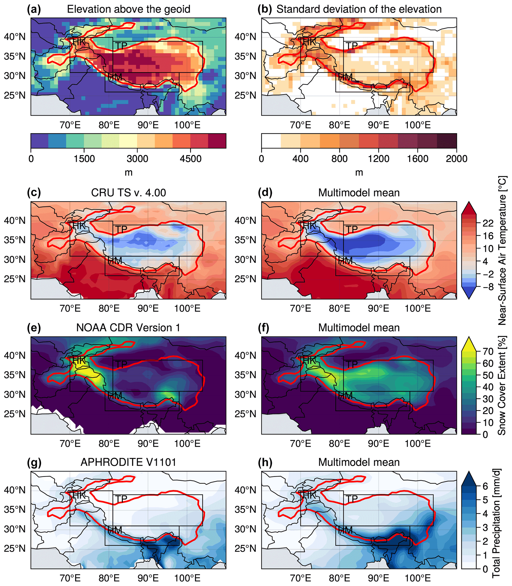
Figure 1Surface elevation (a) and its standard deviation (b) estimated from GMTED2010 at 1∘. Annual climatologies computed over 1979–2014 for temperature (c, d), snow cover (e, f) and precipitation (g, h); the left panels correspond to the observations from CRU (c), NOAA CDR (e), and APHRODITE (g), while the right panels (d, f, h) correspond to the multimodel mean (using the first realization of each ensemble model). The red contour highlights the HMA domain limited to areas higher than 2500 m a.s.l., and the black boxes define the subdomains Hindu Kush–Karakoram (HK), Himalayas (HM), and the Tibetan Plateau (TP), which are also limited to areas higher than 2500 m a.s.l. (red contour) in this study.
Snow cover extent is heterogenous over HMA (Fig. 1e), with high values over HK reaching more than 70 %, which are explained by strong winter snowfalls related to WDs (Cannon et al., 2015; Bao and You, 2019). Snow cover extent is much smaller over most of the TP region, with annual values not exceeding 20 %. High values, around 50 %, are also found over Tien Shan and the southeastern Himalayas. In the multimodel mean (Fig. 1f), snow cover is overestimated over most of the TP and slightly underestimated over the HK region in comparison with the observations.
Strong precipitation rates, reaching an annual mean of more than 6 mm d−1(exceeding 2000 mm yr−1), are observed in the eastern part of HM, mostly due to the Asian summer monsoon, with a decreasing influence from the southeast to the northwest Himalayan chain (Fig. 1g). In contrast, the HK region receives moisture from both Asian summer monsoon and WDs (Fig. 2j). Moisture-laden westerly winds are intercepted by high mountain ranges in northern Pakistan, leading to moisture condensation and precipitation at high elevation (Palazzi et al., 2013), partly explaining the high values of snow cover in this area (Fig. 1e). Due to the orographic barrier, the TP located more on the east is much drier, with annual mean precipitation generally lower than 1 mm d−1. The multimodel mean (Fig. 1h) shows globally higher values of precipitation over HMA in comparison with the observations. Precipitation tends to spread more over the TP in the model compared to the observations, which might be partly due to the smoothing of the topography in the models. However, precipitation rates are also generally underestimated in observational datasets because of snowfall undercatch issues, which could lend credence in the stronger precipitation rates modeled at high elevation.
3.2 Temperature, snow cover and precipitation annual cycle
The seasonal cycles are shown in Fig. 2 for the models and different observational datasets and reanalyses over HMA and the three subdomains for temperature, snow cover and precipitation. The model biases with respect to observations are stronger in winter than in summer for temperature and snow cover, a feature already noticed in CMIP5 and CMIP6 (e.g., Su et al., 2013; Zhu and Yang, 2020). Indeed, the multimodel mean temperature is around 2 to 3 ∘C below the CRU observations in winter over HMA, while models and observations are much closer in summer (Fig. 2a). These differences are more pronounced in the HK region (Fig. 2b) with differences noticed both in winter (4 to 5 ∘C) and summer (∼2 ∘C). The cold bias appears in the multimodel mean (dark blue line) from October/November onwards, peaks between December and January, and then decreases until April/May, except in the HK area where the bias persists in summer. Nevertheless, the multimodel spread encompasses the observation and reanalyses datasets, suggesting a certain reliability of the CMIP6 models. This spread, denoted with the confidence intervals at 50 % and 90 % of the multimodel ensemble (dark and light shadings), highlights a higher dispersion between the models in winter than in summer, except for the HK region. It can be assumed that the larger biases in winter may be due to excessive snowfall, leading to larger snow cover which can amplify the phenomenon. Furthermore, due to the poor representation of fine-scale topography, one can assume that most of the moisture fluxes condense on the plateau at higher elevations, favoring snow precipitation, instead of precipitating earlier on the mountainside. The greater difference in the HK region can be supported by this later hypothesis, knowing that this area is particularly subject to winter WDs bringing a large amount of snow precipitation on the reliefs. Alternatively, it may also be due to the fact that there are very few weather stations in this area, especially at high elevation, and therefore the interpolated CRU data may be overestimated compared to the actual values (Gu et al., 2012). More details on the possible links between the biases are explored in Sect. 3.4.
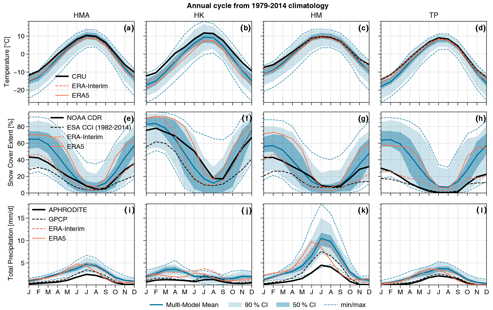
Figure 21979–2014 climatology of the annual cycle of temperature (a–d), snow cover (e–h) and precipitation (i–l) averaged over HMA (a, e, i) HK (b, f, j) HM (c, g, k) and TP (d, h, l), excluding the surface area located below 2500 m a.s.l. (red contours in Fig. 1). The multimodel mean (dark blue line) is shown with the 50 % confidence interval (CI, dark blue shading), the 90 % CI (light blue shading) and the minimum and maximum (dashed blue lines) of the ensemble. The black curves correspond to the observational datasets: CRU, NOAA CDR and APHRODITE, respectively, for temperature, snow cover and precipitation. The ERA-Interim and ERA5 reanalyses are shown, respectively, with the dashed and solid orange curves. GPCP and ESA CCI datasets are also shown for snow cover and precipitation respectively (dashed black line). The ESA CCI covers only the 1982–2014 period.
In comparison with the NOAA CDR satellite observation, the multimodel mean snow cover over HMA is overestimated by 20 % in winter and is closer to the observations in summer when snow cover is lowest (Fig. 2e). The model spread is larger for snow cover than for temperature and precipitation, with values varying from 20 % to 90 % in winter and 0 % to 40 % in summer. This large spread highlights the difficulty to simulate snow cover in complex topography areas and also the large internal variability of snow cover. ERA-Interim is again very close to the observations for snow cover, likely because of the assimilation of IMS data in this reanalysis, a satellite product also used in the production of the NOAA CDR dataset (Drusch et al., 2004; Robinson et al., 2012). The more recent ECMWF reanalysis of ERA5 shows an overestimation of snow cover that is comparable to the CMIP6 model ones. This behavior has already been described in Orsolini et al. (2019), explaining this difference by the fact that ERA5 does not assimilate IMS data beyond 1500 m a.s.l., while Hersbach et al. (2020) suggests that the single-layer snow scheme does not allow enough melting in mountainous regions. The differences found over the three subdomains are similar to those highlighted over the whole HMA (Fig. 2f–h). Nevertheless, we note a precocious spring melt in the multimodel mean and ERA-Interim compared to the NOAA CDR observations and ERA5 in HK region (Fig. 2f). The ESA CCI product shows lower snow cover values compared to NOAA CDR and ERA-Interim, with values around 30 % during the winter in HMA, suggesting that model biases may be even larger. The large difference in spatial resolution with the latter product may also play a role in this discrepancy, as valleys and other aspects of fine-scale topography are not being well resolved in the other products and thus lack a good representation of the spatial heterogeneity of snow cover compared to the ESA CCI product. This suggests a general snow cover overestimation in both model and reanalysis data based on coarse resolution, which is especially pronounced over high mountain areas (Fig. 2f, g). Nevertheless, the positive bias of snow cover fraction simulated by the models over HMA is mainly related to the overestimation of the snow cover over TP, where the snow cover varies around 20 % for the observations, while values above 60 % are found in the multimodel mean, despite a wide dispersion among the models (from 20 % to 90 %).
The strongest precipitation rates occur during the Asian summer monsoon over the HM region (> 2500 m), with precipitation rates reaching a monthly mean of 10 mm d−1 (∼ 300 mm month−1) on average in the multimodel mean, while precipitation rates reach lower values than 2 mm d−1 during the winter (Fig. 2k). Other regions exhibit smaller precipitation amounts below 5 mm d−1 most of the year. In the HK region, larger precipitation rates are found in late winter and spring (Fig. 2j) mostly due to WDs, as explained in Sect. 1. While the model spread generally encompasses the observations for temperature and snow cover, APHRODITE precipitation data are most of the time below the minimum of the model values. This difference might be explained by snow undercatch issues typically obtained with rain gauge measurements (e.g., Jimeno-Sáez et al., 2020), whereas models are expected to provide both solid and liquid precipitation. In addition, rain gauge measurements are generally too sparse to estimate the heterogeneous distribution of precipitation over complex topography areas. Over HK, a large part of the precipitation falls as snow in winter, a period when strong differences between satellite/rain gauge products (black curves) and models/reanalyses are also appearing during February to May, whereas the precipitation is closer between models and observations during the summer (Fig. 2j). Nevertheless, GPCP data (dashed black line) are slightly closer to the models, especially over the HM domain. ERA5 has an early precipitation peak in June, while it is found in July for the other products. Precipitation datasets should be considered carefully knowing that there is no better product than the other ones in this region, and the effective values of precipitation rates are highly uncertain in this area (Palazzi et al., 2013).
3.3 Spatial biases
The pattern of the temperature bias widely differs from one model to another (Fig. 3). However, most of the models show a cold bias, which is reflected by the multimodel mean reaching an average bias of −1.9 [−8.2 to 2.9] ∘C. The cold bias show common general features among the models, being generally more pronounced at high elevation (Fig. 1a), in particular over the HK region, as highlighted in Sect. 3.2. The largest biases are found for the CNRM and IPSL models, with biases reaching almost −10 ∘C on average and exceeding −12 ∘C locally, especially over the western part of the TP and in the Karakoram area (HK region). The other models show slight positive or negative biases around ±3 ∘C. Some models show a positive bias at the edges of the plateau and over Tien Shan (e.g., CESM2-FV2 and MIROC-ES2L) which contrasts with a cold bias on the southern flank of the Himalayas. This is probably due to the low resolution of these models which does not allow to catch the atmospheric circulation over this high-elevation narrow area (Fig. 1b). The cold bias found in a large number of models is more pronounced in winter, a season during which it extends over almost the entire TP, whereas it is limited to the HK region in summer (not shown). Conversely, the warm bias found in some models is reduced in winter and exacerbated in summer.
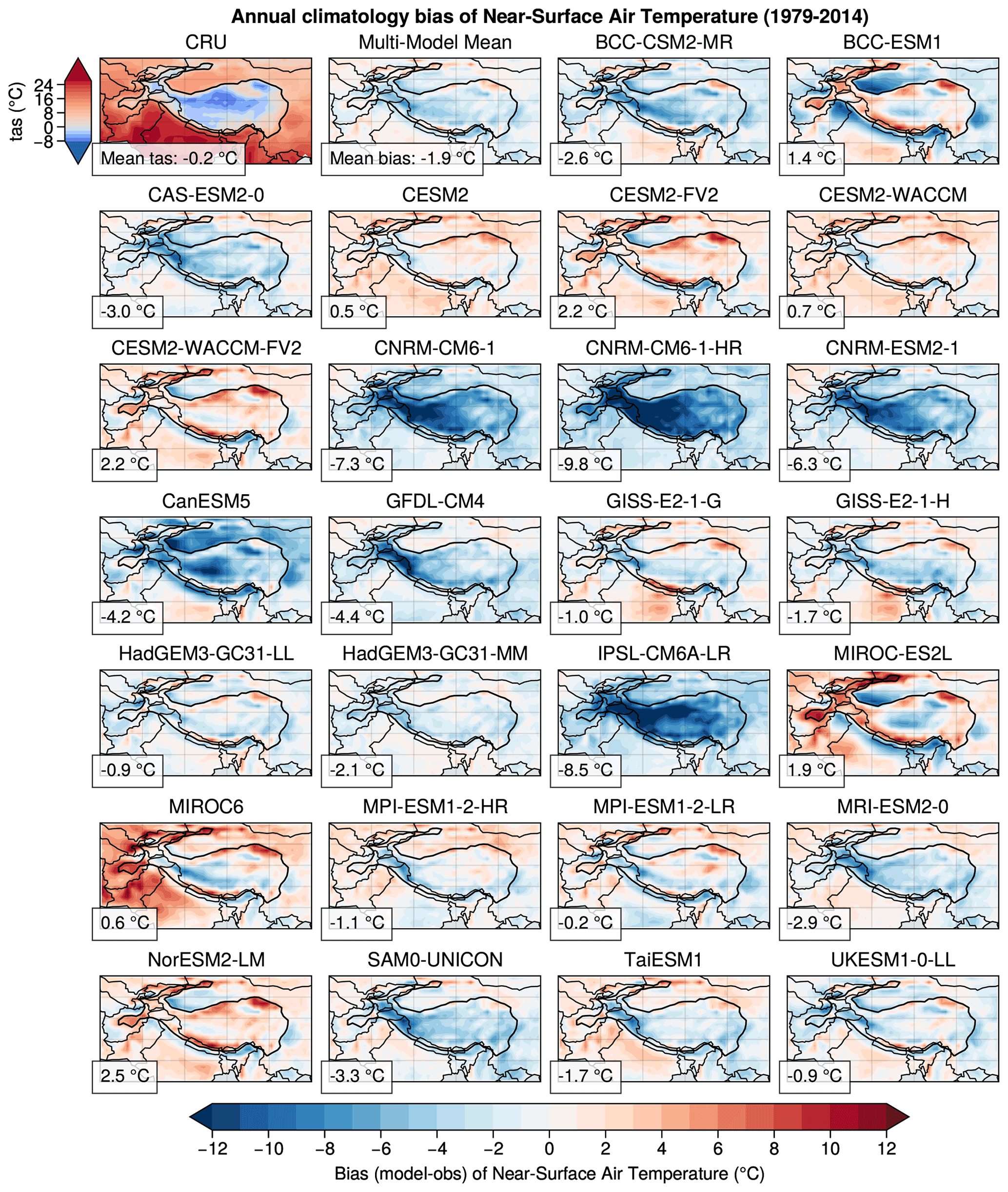
Figure 3Annual bias (model minus observation) computed over 1979–2014 for temperature, except the top left panel that shows the climatology estimated from the CRU observation, used as the reference for the bias computation. The panel located at the right side of the CRU observation shows the bias of the multimodel mean based on the 26 models shown in the figure. The black contour shows the political frontiers and the bold black line the HMA domain located above 2500 m a.s.l., for which the spatial average of the bias is given in the bottom left of each panel.
As for temperature, the snow cover shows a general overestimation in the multimodel mean that extends homogeneously over the whole TP with slightly higher values northwest of TP and over HM (> 30 %) (Fig. B1). Surprisingly, the multimodel mean shows a slight underestimation of snow cover of about 10 % over the HK region, which seems contradictory with the intense cold bias pointed out simultaneously in this area. Indeed, the CRU dataset may overestimate temperature in this area due to a lack of observations, while the low resolution of the NOAA CDR simple binary product (grid cells with or without snow) might overestimate the snow cover in this often snowy area. The ESA CCI product shows a lower snow cover in general and in particular in this region (not shown). It is therefore possible that in the HK region the model biases actually reflect observation deficiencies, even if other factors affecting the model skill could be involved. The annual multimodel mean of snow cover is overestimated by 12 % [−13 % to 43 %], corresponding to a relative bias of 52 % [−53 % to 183 %] over HMA compared to NOAA CDR and can reach locally an absolute difference of 40 %, while a minority of models show a slight underestimation of snow cover (e.g., MPI-ESM1-2-HR, MPI-ESM1-2-LR, NorESM2-LM). The annual overestimation of the snow cover in most models arises mainly from a overly wide extension in the inner TP in winter (not shown). While the excess of snow melts in summer in most of the models, leading to a moderate bias during this season (Fig. 2), some models keep a persistent excess of snow even in summer (e.g., HadGEM3-GC31-LL, HadGEM3-GC31-MM and IPSL-CM6A-LR), which partly explains the large dispersion between the models in terms of annual biases.
All models show higher precipitation rates in comparison with APHRODITE (Fig. B2), as seen in the annual cycles (Fig. 2). Indeed, the multimodel annual mean bias of precipitation over HMA is 1.5 [0.3 to 2.9] mm d−1, corresponding to a relative bias of 143 % [31 % to 281 %]. The bias pattern in terms of total precipitation is somehow proportional to the climatological pattern of precipitation, with stronger biases in the southeastern Himalayas, where high precipitation rates are observed (Fig. B2). The quantification of the bias should be considered carefully for precipitation, because the APHRODITE dataset strongly underestimates the precipitation rates at high elevations (Immerzeel et al., 2015). Anyway, the dry bias found in the southern flank of the Himalayas, coupled with a positive bias of precipitation over TP, suggests an overly coarse resolution to represent the orographic barrier that blocks the northward moisture flux, a limitation especially pronounced during the Asian summer monsoon that induces strong precipitation rates in the south of HMA.
3.4 Spatial bias correlation
To investigate the potential links between the biases of the different variables, the correlation patterns between the biases of temperature, snow cover, precipitation and surface elevation are shown in (Fig. 4). For most of the models, a significant negative correlation is found between the biases of temperature and snow cover, highlighting the influence of these two variables on each other. However, it is not possible to deduce whether it is the snow cover bias that induces the temperature bias or the opposite. The strongest correlations between temperature and snow cover are found for the IPSL-CM6A-LR and the MIROC-ES2L models, suggesting that these biases are exacerbated by feedbacks between these two variables, while lower correlations are found with precipitation biases. On the contrary, some models (e.g., HadGEM3-GC31-MM) show a surprisingly positive correlation between temperature and snow cover, suggesting that other processes can play a role in the development of biases (aerosol deposition on snow, cloud cover, tropospheric biases, etc.).
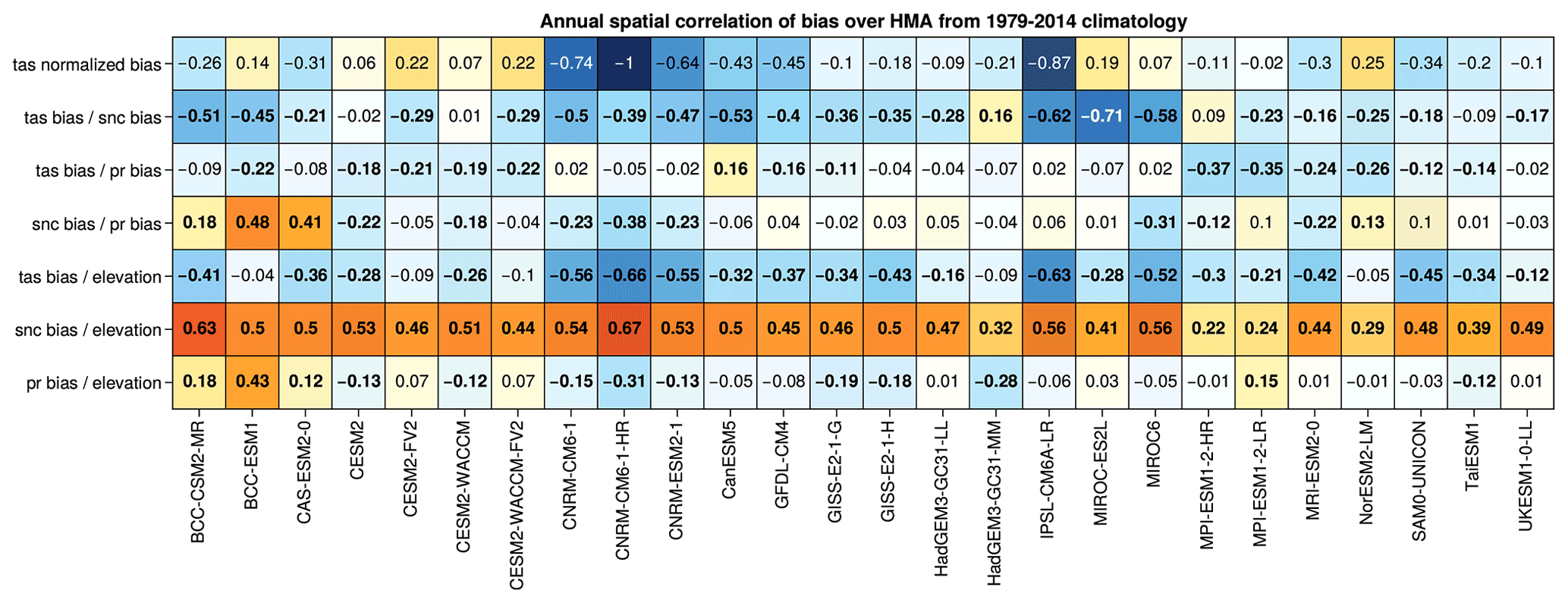
Figure 4Pattern correlations of the annual model biases. The first row shows the temperature bias normalized with the strongest temperature bias found among the 26 models (CNRM-CM6-1-HR). The following rows show the pattern correlations computed between temperature and snow cover biases (second row), temperature and precipitation biases (third row), snow cover and precipitation biases (fourth row). The fifth to the seventh rows show the correlation between biases and surface elevation estimated from GMTED2010 for temperature, snow cover and precipitation. All biases are annual and computed over 1979–2014. Bold characters highlight significant correlation (p value < 0.05).
The correlations between the biases of temperature and precipitation are generally weaker but with negative and significant values between −0.12 and −0.37 (except for CanESM5, which has a positive correlation of 0.16). This seems counterintuitive as we generally expect precipitation rates to increase with temperature unless dynamical changes of the atmosphere could induce an opposite signal at the regional scale. However, the positive precipitation model biases are likely due to the underestimation of solid precipitation in the APHRODITE observation, which would suggest an unrealistic excess of precipitation in the models. Therefore, these negative correlations are potentially not reliable and have to be considered carefully. The comparison with GPCP shows correlations between the biases of temperature and precipitation that reach positive values for a higher number of models Fig. C1. These correlations would likely be more positive if we used an observational reference dataset that was not affected by snow undercatch issues. Nevertheless, the BCC-ESM1 and CAS-ESM2-0 models show a strong correlation between snow cover and precipitation biases (0.48 and 0.41, respectively). This link is particularly striking for CAS-ESM2-0, for which the biases of snow cover and precipitation show similar patterns over the TP and HM (Figs. B1 and B2), suggesting that snow cover biases in that case are partly due to an excess of precipitation.
The temperature and snow cover biases correlations with the surface elevation show a more uniform behavior among the models. In general, an anticorrelation between temperature bias and elevation is found, whereas snow cover correlates positively with the elevation. The higher the elevation, the greater the biases for temperature and snow cover, suggesting that the models have difficulty representing physical processes at high elevation. The link between precipitation bias and elevation is less pronounced with fewer significant correlations (e.g., BCC-ESM1, CNRM-CM6-1-HR, HadGEM3-GC31-MM), which can either be positive or negative.
These spatial correlations are of course region and season dependent. For example, we observe stronger correlations between precipitation and snow cover biases in winter over TP, while the latter is stronger in summer over HK for most of models (Figs. C2 and C3). This may be related to an excess of moisture supply over TP in winter, due to the lack of orographic barrier effect because of the coarse resolution of the models, resulting in too much snow accumulation, which is more likely to persist due to winter cold temperatures over the TP. Concerning the excess of summer precipitation in HK, this may be due to an overextension of precipitation towards the west of the Himalayan mountain range during the monsoon period. However, this last correlation, supporting the idea that the excess snow cover may be due to excess precipitation for some models, does not necessarily explain the cold bias at the surface. For example, the HadGEM3 models have strong significant correlations between snow cover and precipitation biases over the TP (0.63 and 0.66 annually) but do not show a significant surface cold bias (−0.12 and −0.18 ∘C; Fig. C3). The relationship of the biases with altitude is not always verified either, especially for models showing warm biases such as the CESM2 family of models over the TP in summer.
3.5 Metrics
Spatial RMSE and mean biases are computed over HMA for the 26 models (Fig. 5). CESM2, CESM2-WACCM and MPI-ESM1-2-HR show the lowest temperature RMSE (∼ 2.5 ∘C), with a mean bias smaller than 1 ∘C, while worse performing models are CNRM-CM6-1, IPSL-CM6A-LR and CNRM-CM6-1-HR with RMSE exceeding 7 ∘C. The best models for temperature are not necessarily the best ones for snow cover and precipitation (e.g., HadGEM3-GC31-LL, HadGEM3-GC31-MM, UKESM1-0-LL). RMSE for snow cover ranges from about 10 % to 45 %, and most of the models show a positive snow cover bias over HMA. RMSE for precipitation ranges from over 1 to 3.5 mm d−1, while mean biases are all positive, ranging from about 0.5 mm d−1 to slightly over 2 mm d−1 (Fig. 5c), as we already discussed in Sect. 3.3.
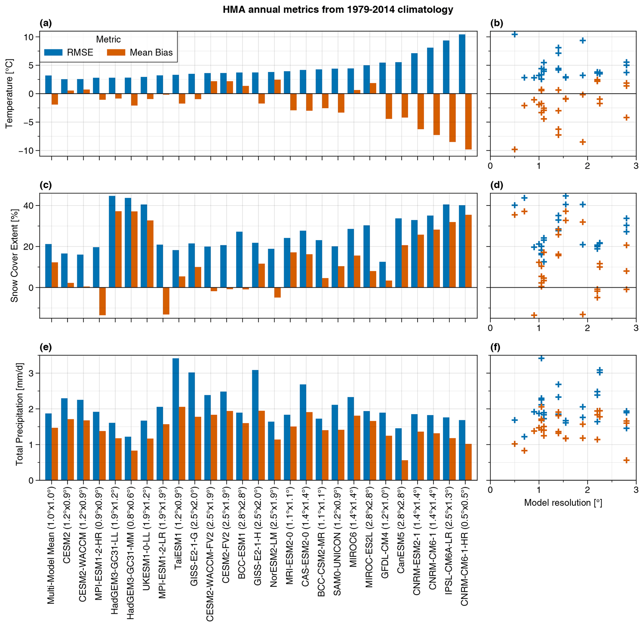
Figure 5Annual spatial RMSE and bias computed over HMA with respect to CRU, NOAA CDR and APHRODITE, respectively, for temperature, snow cover and precipitation (a, c, e). Models are ranked by increasing RMSE for temperature and the multimodel mean appears in the first histogram. The approximate original model's resolution is given, but all metrics are computed on a common 1∘ × 1∘ grid after interpolation. Panels (b, d, f) are similar to (a, c, e) with models ranked as a function of their original mean lat/long resolution. Blue and red crosses correspond respectively to RMSE and mean bias.
On the right panels of Fig. 5 (b, d, f), the RMSE and mean bias are ranked by model resolution. Finer-resolution models do not show better skill for temperature, snow cover and precipitation, suggesting that GCM resolution is not the more important criterion for climate modeling over this region. This general assumption is not the case for all model families. For example, MPI-ESM1-2-LR (1.9∘ × 1.9∘) and MPI-ESM1-2-HR (0.9∘ × 0.9∘) do show slight improvements for all variables with increasing resolution. However, for CNRM-CM6-1 (1.4∘ × 1.4∘) and its high-resolution version CNRM-CM6-1-HR (0.5∘ × 0.5∘), the increase in resolution leads to a degradation for temperature and snow cover, while there is a slight improvement for precipitation.
The Taylor diagram (Taylor, 2001) shown in Fig. 6 is used to investigate the realism of the spatial variability simulated in the models as compared to observational references. Overall, the models perform better for temperature than for precipitation, whereas the model skill is even smaller for snow cover. The pattern correlation (PCC) ranges from 0.7 to 0.9 for temperature, whereas it takes lower values for precipitation varying from 0.6 to 0.8 for most of the models, except for HadGEM3-GC31-MM, for which it reaches 0.9 and for five other models showing a lower PCC below 0.6. For snow cover, the model PCC is even lower and also heterogeneous among the models, varying from negative values (−0.17 for MIROC-ES2l) to a maximum of 0.8 (GFDL-CM4). Overall, the spatial variance is higher for almost all the models as compared to observations for both the temperature (the normalized standard deviation reaching 1.5 for the worst model) and the precipitation (the normalized standard deviation exceeding 4 for the worst model). This is the contrary for snow cover, a variable for which the models show smaller spatial heterogeneities in comparison to the observational reference, with a normalized standard deviation generally lower than 1, and varying between 0.4 and 1.4 for all the models. The larger temperature standard deviation found for the models is partly explained by the general cold bias over HMA that enhances the temperature contrast between the high-elevation areas and the surrounding plains. The excess of precipitation found in the models over the area located under the influence of the Asian monsoons also explains the high standard deviation found in the models for this variable. In contrast, the low standard deviation found in the model for the snow cover is likely related to the overly extended and overly homogeneous snow cover over TP and its surrounding mountains, while the TP in observations is most often free of snow. Another interesting point is that both ERA-Interim and ERA5 do not perform much better than the CMIP6 models (except ERA-Interim for temperature and snow cover likely due to IMS snow cover assimilation over HMA), suggesting general weaknesses in the models used commonly for climate modeling and for the production of atmospheric reanalysis, while the multimodel mean has intermediate performance among the models.
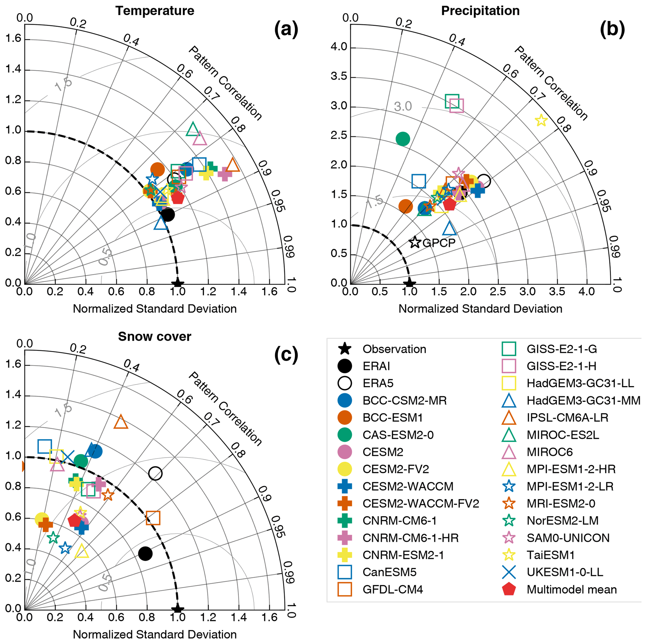
Figure 6Taylor diagram showing for the 26 models over HMA the 1979–2014 mean of the spatial pattern of temperature (a), precipitation (b) and snow cover (c). The observational reference is shown with a black star corresponding to CRU (temperature), APHRODITE (precipitation) and NOAA CDR (snow cover extent). ERA-Interim and ERA5 are shown with the black circles filled and unfilled, respectively. The red pentagons correspond to the multimodel mean. The radial distance from the origin is proportional to the area-weighted standard deviation of the spatial pattern (normalized by the observation standard deviation). The area-weighted normalized centered RMSE between the model and the reference is proportional to the distance from the black star (light gray semi-circles). The area-weighted pattern correlation coefficient between the two fields is given by the azimuthal position.
Overall, it is challenging to discard any model from this spatial analysis, as well as RMSE and bias metrics, because of both a large heterogeneity of skill found among the models and a skill that varies also from one variable to another for the same model. This finding suggests that there is no reason to exclude some models for climate analysis purposes in this area in particular when looking at future projections. Nevertheless, to explore this question deeper, the potential relationship between biases and trends is investigated in Sect. 4.2.
Disentangling the trends related to internal variability from the forced signals related to anthropogenic forcing is challenging. At midlatitudes, internal variability can contribute until 50 % to climate trends computed over 50 years (Deser et al., 2020). However, this contribution decreases when considering areas closer to the tropics and when integrating climate signals over large domains (Hawkins et al., 2016). The climate trends in HMA are explored over the period 1979–2014 by comparing observational datasets and multimodel mean computed with a single member for each model to give the same weighting to each model (Fig. 7). This comparison should be considered carefully, since observational datasets reflect the superposition of both the internal variability and the forced signals whereas the internal variability is partly filtered out when averaging the model outputs. However, the 35-year period considered here is supposed to be long enough to exclude a large part of the internal variability. The spatial comparison between models and observations is used in Sect. 4.1 to investigate forced signals and model deficiencies at the regional scale.
The modulation of the trends by internal variability is explored in Sect. 4.2, where trends are spatially integrated separately for each ensemble member to investigate the contribution of internal variability and to investigate the potential impact of model biases on simulated trends.
4.1 Trends
Figure 7 shows a general positive trend for temperature in observations and models during both seasons. Shading highlights the significant trends (p value > 0.05), contours are used for non-significant trends, and we consider that trends are robust when > 80 % of the models agree on its sign (hatching). In winter observations, stronger temperature trends are found over the TP with values ranging from 0.3 to 0.6 ∘C decade−1 over 1979–2014, while weaker warming occurred over the Indo-Gangetic Plain downward of HM, with values not exceeding 0.3 ∘C decade−1 (Fig. 7a). The multimodel mean shows slightly lower values of temperature trends in winter than the CRU observations, except for the northern HMA. Summer temperature trends show a similar pattern as the winter ones but with the highest values over the western part of TP, reaching 0.5 ∘C decade−1 in the model, while the CRU observations show a northward shift of the positive trends close to the Tarim Basin. The temperature change found in CMIP6 models and observations is consistent with previous estimations (e.g., Wang et al., 2008; Liu and Chen, 2000) and has also been highlighted in ERA-Interim and ERA reanalyses with slightly different patterns (Fig. D1).
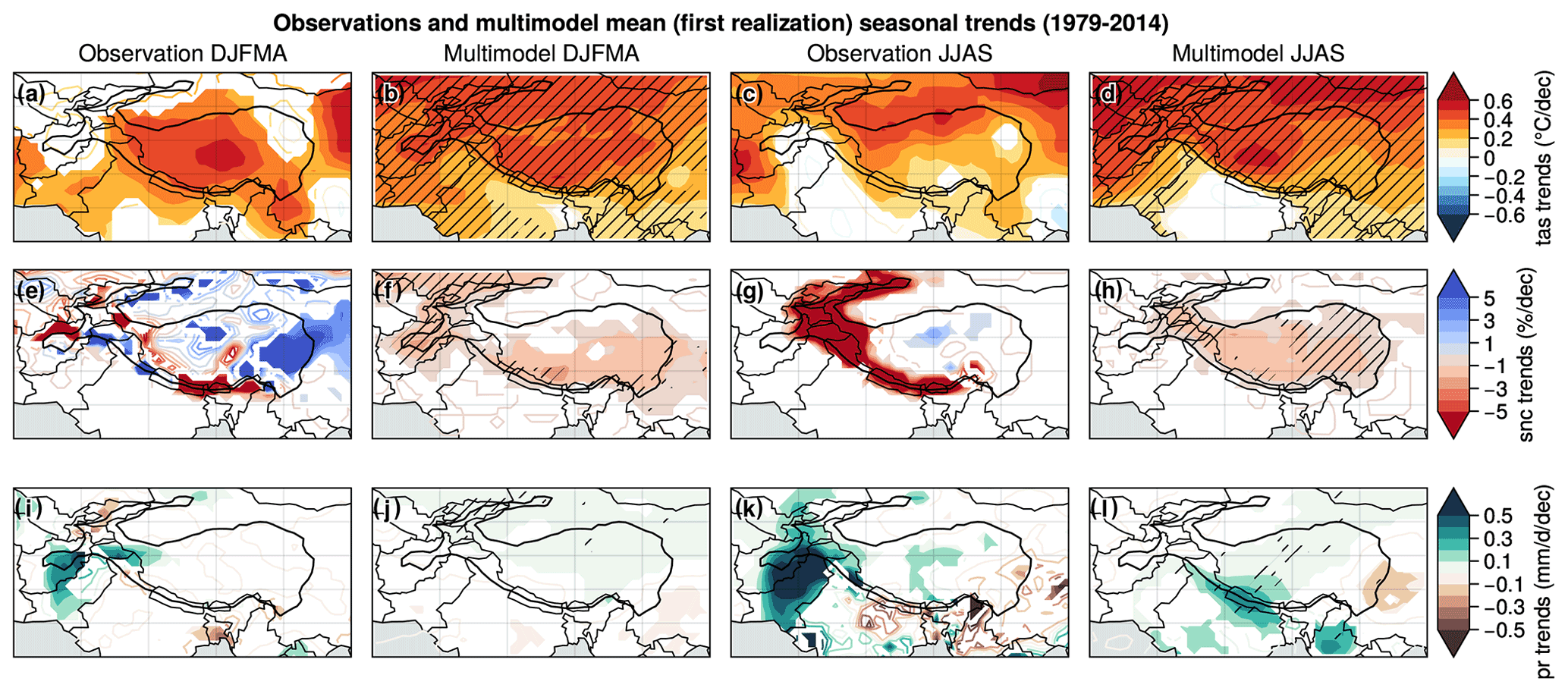
Figure 7DJFMA (left) and JJAS (right) trends computed over 1979–2014 for temperature (a–d), snow cover (e–h) and precipitation (i–l). CRU temperature, NOAA CDR snow cover and APHRODITE precipitation observation trends (DJFMA: a, e, i and JJAS: c, g, k) are compared to the multimodel mean computed with the first realization for each model (DJFMA: b, f, j and JJAS: d, h, l). Contours are used for non-significant trends, shading for significant trends (p value > 0.05) and hatching for points where > 80 % of the models agree on the sign of the trend.
There are more discrepancies between models and observations for snow cover (Fig. 7e–h). The multimodel mean shows a slight significant and robust decreasing trend of snow cover in both winter and summer, reaching −1 % decade−1 to −2 % decade−1 over most of HMA (Fig. 7f, h), while observations show more pronounced trends with a spatially heterogeneous pattern in winter (Fig. 7e) and a significant decline in snow cover in summer over the whole Himalayas, extending to HK and Tien Shan, with values exceeding −5 % decade−1 (Fig. 7g). Meanwhile, the observation show slightly positive trends for the TP. However, the snow cover trends observed in the NOAA CDR dataset should be taken with caution, due to the poor resolution (∼ 200 km), which is problematic for mountain areas (Bormann et al., 2018).
Observed trends are generally less significant for precipitation than for temperature. The large interannual precipitation variability limits the possibility to detect long-term trends for this variable. This also explains the discrepancy between the observation and the multimodel mean for precipitation (Fig. 7i–l), with signals that show a larger amplitude in the observation than in the multimodel mean where the internal variability has been filtered out by averaging several model outputs. In the observations, the main precipitation signal is a significant increase in HK during both seasons (more pronounced in summer), which extends southward in the Indo-Gangetic Plain during the summer, ranging from 0.1 to 0.5 mm d−1 decade−1 (Fig. 7i, k). This pattern is not found in the multimodel mean, whereas an increase in precipitation is simulated during the summer but shifted eastward over HM in comparison with the observation, with values between 0.1 and 0.3 mm d−1 decade−1 (Fig. 7j, l). This summer signal is likely related to monsoon changes, with patterns that differ however between models and observations. During both seasons, the multimodel mean suggests a robust and significant increase in precipitation over TP, with values around 0.1 mm d−1 decade−1. This signal is consistent with the observation during the summer, albeit less pronounced in the model with respect to the observation, whereas there is no clear change of precipitation during the winter in the observations. Nevertheless, caution is required when considering observations of precipitation that are generally uncertain because of undercatch issues for solid precipitation (see Sect. 2.2.3). The discrepancy between different observational datasets and reanalysis trends illustrated in Fig. D3 confirms the strong uncertainty typically found in precipitation datasets. Nevertheless, a summer signal is clearly visible in both models and observations, potentially related to monsoon changes, with an increase in precipitation rates over wide areas of the western part of HMA and the Indian subcontinent that is modulated by drying patterns located more on the east, which spatially diverge among the different products.
4.2 Trends versus bias
Figure 8 shows the ensemble trends versus the ensemble biases for each model. Most model spreads (vertical bars) generally overlap the range of the observed trends (black shading). This suggests that the forced plus the internal variability estimated with the model ensemble is compatible with the observed variability. A few model spreads stand outside of this range and should be considered carefully. However, the observed trends can also be affected by artifacts as discussed in Sect. 4.1 and are not fully reliable either. In addition, some models include only a limited number of members, sometimes a unique one (Table A1), so the ensemble for these models does not cover the full range of plausible evolutions. Some highly biased models fall within the range of observed trends, whereas others show a combination of small biases and unrealistic trends. This finding suggests that model bias is not a robust criterion to discard models in trend analysis.
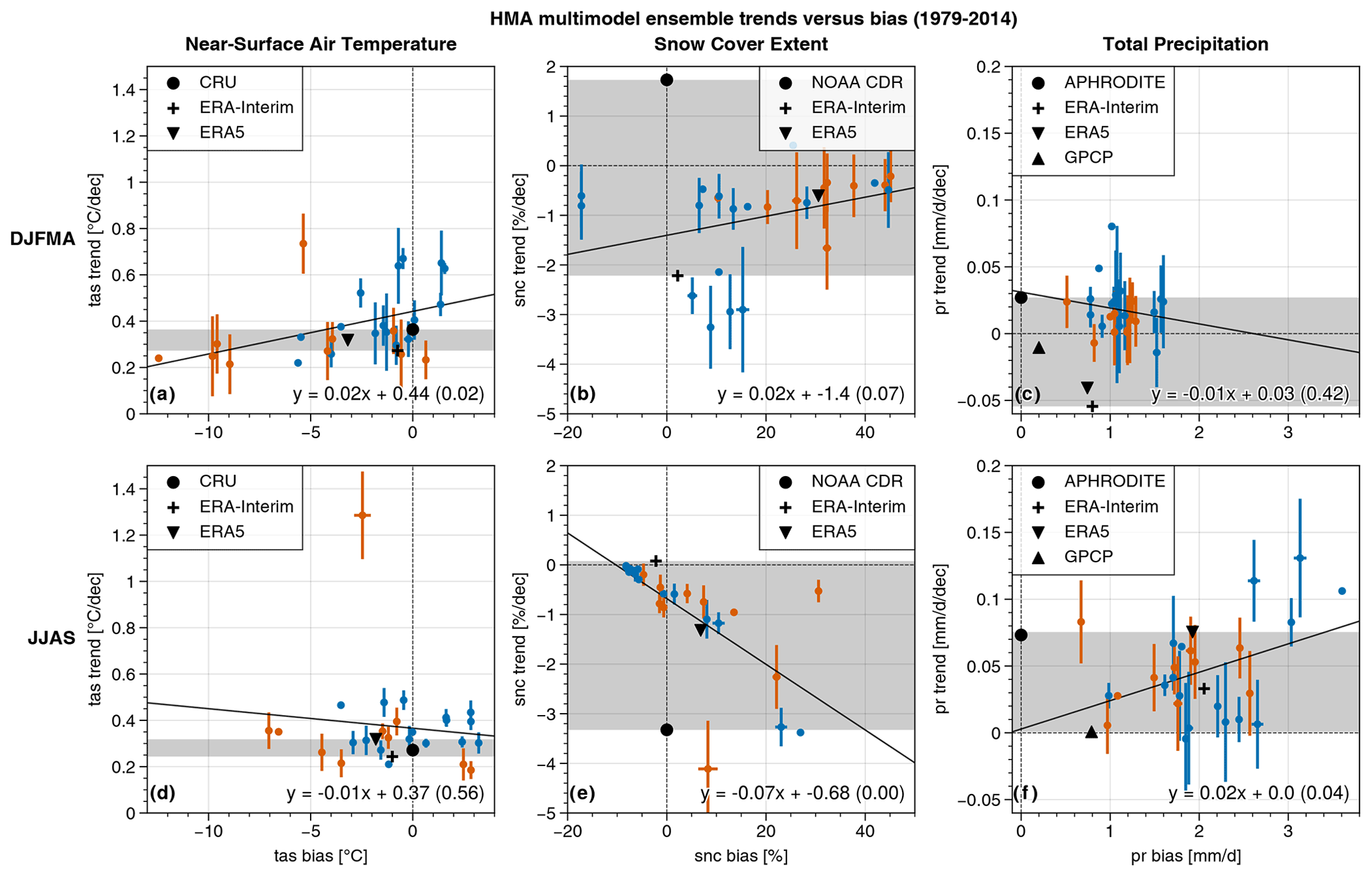
Figure 8Seasonal (DJFMA and JJAS) HMA multimodel ensemble trends versus model biases over 1979–2014 for temperature (a, d), snow cover (b, e) and precipitation (c, f). Vertical (horizontal) bars correspond to the standard deviation of the trends (biases) of the ensemble members for each model (the number of members differs among the models Table A1). Observation and reanalysis datasets are shown with black symbols. The 10 models used for projections are shown in orange, while other models are shown in blue. The gray shading represents the range of observation trends. The solid black line corresponds to a linear regression from the multimodel mean values (including all models) with the p value shown in brackets following the equation at the bottom right of each panel. The light horizontal (vertical) dashed lines correspond to a null trend (null bias with respect to the reference observation dataset).
Nevertheless, even with a large spread, a dependency of the simulated past trends on the model biases is found for some variables and seasons, and in particular for winter temperature, summer precipitation and snow cover during both the winter and the summer. The low values of snow cover in summer over HMA might explain the limited melting for low biased models, whereas the models with large amounts of snow cover persisting in summer show a decreasing trend of snow cover with the warming (Fig. 8e). This is likely to result in an overestimation of summer melting rates. The models overestimating the snow cover during the winter are also showing small decreasing trends of snow cover (Fig. 8b). This is likely related to attenuated warming trends found in cold-biased models during the winter (Fig. 8a), suggesting a damping of the warming in cold models. During the summer, there is no clear relationship between bias and trends of temperature (Fig. 8d), but the models simulating an excess of precipitation rates also show enhanced precipitation increases (Fig. 8f). This might be explained by the non-linear relationship between temperature and atmospheric moisture: at fixed warming rates, the models showing a more active hydrological cycle also show a stronger precipitation increase.
Even with such a relationship between biases and trends, the number of observations is too small and their uncertainties too large to allow a robust selection of the models that could be used in climate analysis. Nevertheless, with more observations available, these results could help to select a subset of models to reduce the spread in future projections for example. Still, the relationship between models and biases is less clear when considering only the 10 models for which the full set of projections is available (orange points). We assume therefore that future trends shown in Sect. 5 are not dependent on the model biases.
It should be noted that one model (CanESM5) used for projections stands out for temperature in both seasons, with values reaching about 1.3 ∘C decade−1 in summer, while for the other models, summer trends range from about 0.2 to 0.5 ∘C decade−1 (Fig. 8d). However, this does not justify discarding this model because recent trends are not unrealistic for other variables and seasons. Nevertheless, one can expect that the upper limit of the temperature projection range will be overestimated because of that model. Because this behavior could affect the multimodel mean, we use the median of the multimodel ensemble instead.
In this section, we use the 10 models for which the four SSP scenarios based on different levels of anthropogenic emissions (SSP1-2.6, SSP2-4.5, SSP3-7.0, and SSP5-8.5) (O'Neill et al., 2016) are available (Table 1).
5.1 Projected changes over HMA
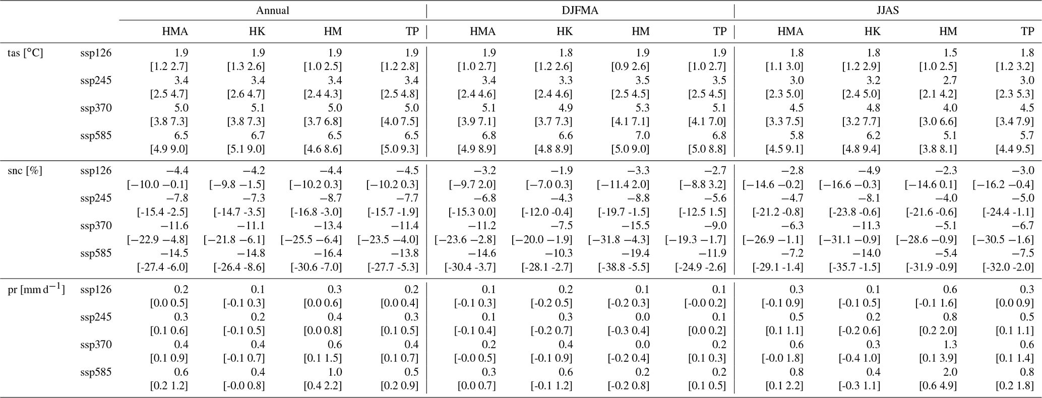
The 10 CMIP6 models project a warming over HMA at the end of this century (2081–2100 with respect to the 1995–2014 average) that ranges from 1.9 [1.2 to 2.7] ∘C for SSP1-2.6 to 6.5 [4.9 to 9.0] ∘C for SSP5-8.5 (Table 2). This warming is expected to continue beyond 2100 under the SSP5-8.5 scenario (Fig. 9), while a stabilization of temperature is simulated under the scenario SSP1-2.6 between 2060 to 2080, followed by a slight cooling. This warming is associated with a snow cover extent decrease ranging from −4.4 % [−10.0 % to −0.1 %] to −14.5 % [−27.4 % to −6.0 %] (Table 2). This absolute change corresponds to a relative loss of −9.4 % [−16.4 % to −5.0 %] to −32.2 % [−49.1 % to −25.0 %] with respect to the 1995–2014 average (Fig. 9b). These changes are concomitant with a precipitation increase from 0.2 [0.0 to 0.5] to 0.6 [0.2 to 1.2] mm d−1, corresponding respectively to a relative increase from 8.5 % [4.8 % to 18.2 %] to 24.9 % [14.4 % to 48.1 %] with respect to the 1995–2014 average. As for temperature, snow cover and precipitation are expected to stabilize under the SSP1-2.6 scenario, while an acceleration of snow cover decrease and precipitation increase is simulated under SSP5-8.5. SSP2-4.5 and SSP3-7.0 show intermediate pathways between SSP1-2.6 and SSP5-8.5. NOAA CDR shows much greater interannual variability compared to the models both in the historical period and the projections; thus, it seems difficult to model the natural variability of snow cover.
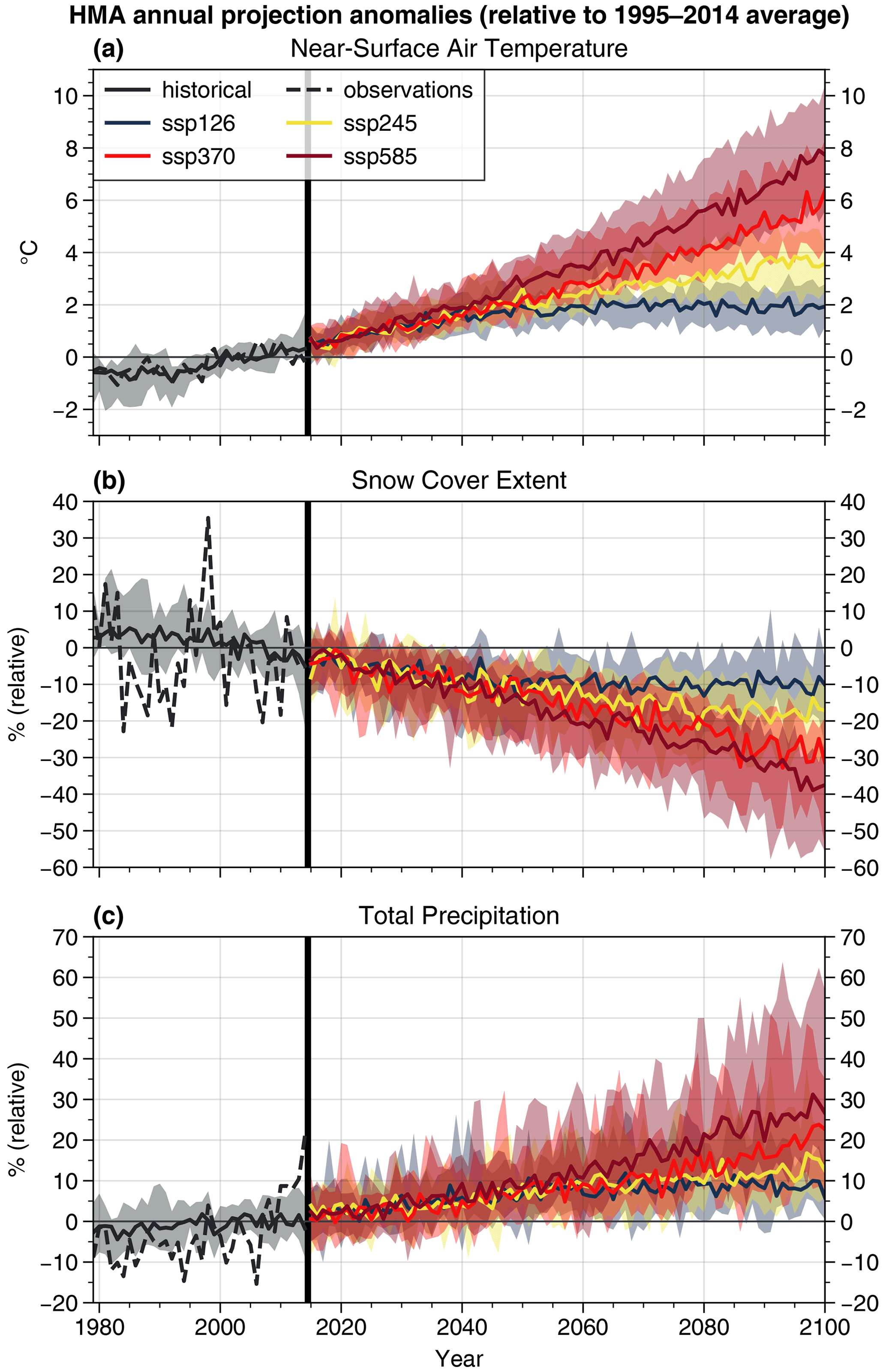
Figure 9Annual yearly anomalies (with respect to the mean computed over 1995–2014) simulated in HMA over 1979–2014 (black curves) and over 2015–2100 under four scenarios: SSP1-2.6 (dark blue), SSP2-4.5 (yellow), SSP3-7.0 (red) and SSP5-8.5 (dark red) for temperature (a), snow cover (b) and precipitation (c). Medians are computed with the first member for the 10 models for which the future projections are available (Table 1). The thick vertical black line delimits the historical and future periods. CRU, NOAA CDR and APHRODITE observations dataset are shown for the historical period in dashed lines, respectively, for temperature, snow cover and precipitation. Shadings highlight the 90 % confidence interval, corresponding to the 0.05 and 0.95 quantiles.
The future warming over HMA is more pronounced in winter than in summer (Fig. 10a–d). These seasonal contrasts are more pronounced in strong CO2 emissions scenarios, with almost no differences for SSP1-2.6 (∼ 0.1 ∘C) to about 1 ∘C under SSP5-8.5 (5.8 ∘C in summer to 6.8 ∘C in winter; Table 2). Enhanced winter warming is associated with a strong decrease in snow cover by −15 % (Fig. 10e–f) located over HK and northward (east side of Tien Shan), HM and southeastern TP. This last reduction of snow cover must be amplified by an early spring melt. The snow cover decrease is smaller in summer and is mainly located in the western part of TP. Snow cover extent is drastically reduced in summer from about −30 % to more than −80 % locally (Table E) and only in the areas where snow cover persists during the summer. Precipitation is projected to increase both in summer and winter. The precipitation increase in winter in HK suggests an intensification of WDs, while the summer increase found over HM and TP corresponds to an increase in monsoon-related precipitation (Fig. 10i–l). The relative increase in precipitation is slightly higher in summer than in winter for the whole HMA domain, ranging from 6.4 % [0.7 % to 13.5 %] to 22.8 % [9.8 % to 45.8 %] in winter and 9.1 % [5.7 % to 20.6 %] to 25.6 % [14.2 % to 50.0 %] in summer, depending on the scenarios (Table E). The changes simulated under the different scenarios show different amplitudes but with similar patterns (Fig. 10).

Figure 10Median of the model differences between the 2081–2100 and the 1995–2014 averages for temperature (a–d), snow cover (e–h) and precipitation (i–l) under the SSP2-4.5 and SSP3-7.0 scenarios. The first realization is used for each model. The black contour corresponds to the HMA domain (> 2500 m) for which the spatial average is shown in the lower left box.
Table 2Annual and seasonal (DJFMA and JJAS) multimodel median anomalies averaged over 2081–2100 (with respect to 1995–2014 average) and their 90 % confidence interval (0.05 and 0.95 quantiles) for temperature, snow cover and precipitation over the full HMA domain and the subregions HK, HM and TP, under the four SSP scenarios: SSP1-2.6, SSP2-4.5, SSP3-7.0 and SSP5-8.5.
5.2 Changes in the HMA region in the global context
HMA is projected to warm around 1.5 times faster than the atmosphere at the global scale, with a quasi-linear relationship between HMA and global surface air temperature (GSAT; Fig. 11a). This stronger signal over HMA is mainly explained by the enhanced warming rates that occur over the continental areas with respect to oceanic regions, since the warming rates affecting the NH continental surfaces and the HMA are similar (Fig. 11b). Nevertheless, the warming rate is stronger over HMA than over the remaining continental areas located south of 60∘ N. This amplification with respect to other tropical to midlatitude areas reaches 11 % and is significant at the 5 % level, and was already noticed in CMIP5 (Rangwala et al., 2013). This is potentially related to feedbacks involving snow cover changes, namely snow–albedo feedback, and other processes specific to mountainous areas. Mudryk et al. (2020) showed that the projected NH spring snow cover extent decrease is proportional to the global temperature change, the slope of the relationship being independent of the scenario. Similarly, the HMA snow cover in DJFMA follows a linear decrease of about 4 % per degree of GSAT increase (Fig. 11d). This relationship does not show a linear behavior in summer, with a curved relationship highlighting small snow cover decrease rates at high levels of global warming (Fig. 11e). The summer curved relationship is explained by a fast retreat of snow cover at low elevation under moderate warming, whereas some snow cover still persists at very high elevation even under strong warming rates. However, almost all the summer snow cover is vanishing in the highest CO2 emissions scenario (SSP5-8.5). The annual precipitation increase also appears to behave linearly with the GSAT increase, with an increase of precipitation slightly higher than 6 % per degree of GSAT increase (Fig. 11f).
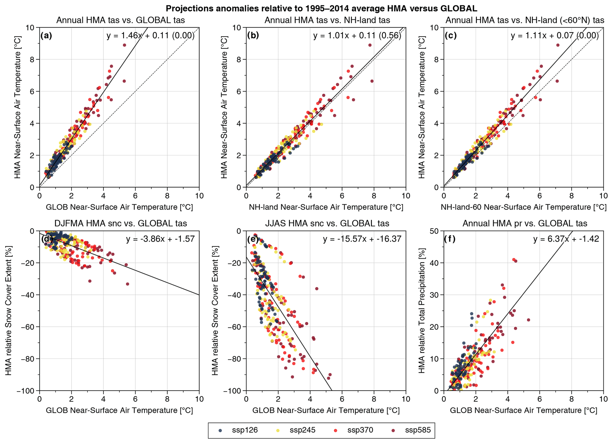
Figure 11Projected anomalies over HMA computed with respect to 1995–2014 averages for the 10 models under the SSP1-2.6 (dark blue), SSP2-4.5 (yellow), SSP3-7.0 (red) and SSP5-8.5 (dark red) scenarios for annual temperature (a, b, c), seasonal snow cover (d, e) and annual precipitation (f) as a function of temperature integrated globally (a, d, e, f) and over NH continental surfaces including (b) and excluding (c) boreal areas (latitude > 60∘ N). Each point on the scatter plots corresponds to a 20-year average computed with 10-year steps from 2015 to 2095. The Global Land Data Assimilation System (GLDAS) Land/Sea Mask Dataset at 1∘ resolution (https://ldas.gsfc.nasa.gov/gldas/vegetation-class-mask, last access: 6 October 2020) is used to mask the continental data in the different models. The dashed line corresponds to the line of equation y=x and the solid black line to a linear regression detailed at the top right of each panel. In the first row (a–c), a significance Wald test is done to test if the observed trend is significantly different from the equation y=x (p value is shown in brackets).
The cold bias over the TP and mountainous areas has been a persistent issue in GCMs since the first AMIP experiments (Mao and Robock, 1998). The mean cold bias found in our study is coherent with previous CMIP5 studies as, for example, Su et al. (2013) that estimated a cold bias of 1.1 to 2.5 ∘C in winter and values not exceeding 1 ∘C in summer. Zhu and Yang (2020) showed an improvement from CMIP5 to CMIP6 with a mean bias reduction reaching 0.44 ∘C. However, the skill changes from CMIP5 to CMIP6 are contrasted among the models. MPI-ESM-LR was the model performing the best over HMA in terms of temperature RMSE in Table 6 of Su et al. (2013), and it is still in the top three models in our study in its high-resolution version, while CanESM2 was in the top five models and dropped down to the five worst models in our study. Even if these results are not directly comparable because the studies do not focus on exactly the same periods, methods and area, this still gives insight on the fact that not all models improved or maintained their ability to simulate temperature over HMA. Deteriorations might be due to some changes in the models. This is, for example, the case for IPSL-CM6A-LR, which contains a new snow scheme (Wang et al., 2013a) that improved snow cover representation over most of NH but increased the biases over HMA (Cheruy et al., 2020).
Indeed, cold bias might be related to a misrepresentation of snow cover in some cases. As noted by Zhu and Yang (2020), the average model temperature bias is more pronounced in winter, suggesting a possible role of snow–albedo parameterizations. However, the bias correlation between temperature, snow cover and precipitation (Fig. 4) indicates that the temperature bias might not only be due to snow cover misrepresentation, in particular for some models that show low correlations between temperature and snow cover (e.g., CAS-ESM-2-0, CESM2), whereas some of them have a high correlation with precipitation. However, all these variables are connected, as an excess of precipitation can induce an overestimation of snow cover and generate a cold bias, but an initial cold bias in the atmosphere could also generate an overestimation of solid precipitation leading to an excess of snow cover. Nevertheless, the correlation between snow cover bias and precipitation bias is less obvious for most of the models. Exceptions are BCC-ESM1 and CAS-ESM2-0, where these variable biases are highly correlated (0.48 and 0.41), indicating in that case that precipitation might be partly the cause of the temperature biases. However, models that display the strongest cold biases, such as CNRM-CM6-1-HR, IPSL-CM6A-LR and CNRM-CM6-1, also show high anticorrelation with snow cover bias (−0.39, −0.62 and −0.5, respectively). This supports the recommendation by Zhu and Yang (2020) to improve snow cover parameterizations in models. In addition, as mentioned by Gu et al. (2012), the lack of high-elevation observation stations in the CRU data may also be partly responsible for the apparent cold bias of the models. Direct comparison from CRU and models can also amplify this bias, knowing that differences of elevation can be noted between GCMs. Therefore, certain studies (e.g., Sheffield et al., 2006; Chen et al., 2017) correct temperatures with a common lapse rate (e.g., 6.5 ∘C km−1) to bring them to the same elevation. However, in our case, where we wanted to correlate the model biases of different variables and see the impact of original model resolution, this method would have introduced additional uncertainties due to spatially heterogeneous lapse rates over this region and partially corrected the biases due to model resolution, making it difficult to compare the variables with each other.
Other variables such as cloud cover and aerosols might also be important factors involved in model biases. Indeed, the aerosol effect on snow cover is often investigated. It induces a reduction of the seasonal snow cover duration of a few days, in particular over HMA (Ménégoz et al., 2014), but regarding the large snow cover biases in models, it might be a second-order issue for highest biased models. However, the spatial imprint of aerosol forcing seems highly correlated with snow cover biases (see Usha et al., 2020 Fig. 7d and Fig. B1 of this paper). Usha et al. (2020) conclude that snow darkening due to aerosols increases the surface temperature by 1.33 ± 1.2 K, which results in the reduction of snow cover fraction by 7 ± 11 %. Therefore, a misrepresentation in aerosols deposition on snow might amplify snow cover biases and/or be the main cause for some models, while the multimodel mean absolute snow cover bias is estimated to 12 % [−13 % to 43 %] in this study. Zhou and Li (2002) and Yu et al. (2004) conjectured that a poor representation of cloud properties might lead to insufficient plateau heating, resulting in a cold bias in the TP. The problem could also arise from a misrepresentation of processes in the boundary layer. Indeed, De Wekker and Kossmann (2015) and Serafin et al. (2020) expose the lack of constraints for processes in the planetary boundary layer over complex terrain, in addition to the limited applicability of existing turbulence theory with frequent violation of its basic assumptions (e.g., stationarity and isotropy of small-scale turbulence) over mountainous areas. Further theoretical and observation work is thus needed to improve model parameterizations over these regions. Chen et al. (2017) focused on the surface energy budget from 28 CMIP5 models and suggested that improvements in the parameterization of the snow cover area and the boundary layer processes should allow reducing the cold bias over the TP. Further research is required to advance scientific understanding about the origins of systematic model biases in the HMA region.
Some models also show temperature biases in the troposphere at a global scale (not shown) that might amplify and/or even trigger surface biases in HMA. Salunke et al. (2019) also highlighted that many models still struggle to capture the large-scale atmospheric circulation, such as the location and intensity of upper-level Asian anticyclone and middle troposphere temperature maximum over the TP, which have large implications on the TP as well as on the Indian summer monsoon. Wrong atmospheric circulation, as the position of jets, could also feed the observed biases in models over HMA. Further analyses in higher atmospheres and circulation must be done to quantify this impact on present biases.
The obvious link between topography, snow cover bias and to a lesser extent the temperature bias (Fig. 4) indicates also the inability of GCMs to simulate key variables over complex topography. Furthermore, increasing the model resolution does not result in a systematic reduction of model biases (Fig. 5b, d, f) because resolutions of 50 km or higher are still too coarse to represent adequately all the physical processes peculiar to the complex topography of the HMA region. Hence, the development of subgrid-scale parameterizations appears essential to better simulate the climate of these regions. As an example, the snow cover extent parameterization is often too simple in actual GCMs. Many GCMs either use a simple linear relationship with snow water equivalent (SWE), as in the ERA-Interim reanalysis, or take also into account a dependency to the snow density as implemented in ERA5 and IPSL-CM6A-LR, for example. However, many models do not include any representation of subgrid-scale processes driven by the local topography, an essential feature for complex topography areas. This idea has been explored a few decades ago (e.g., Walland and Simmonds, 1996; Roesch et al., 2001) and more recently in Swenson and Lawrence (2012) who considered satellite observations to develop a subgrid-scale representation of snow cover with a dependency on the local topography. Such approaches are however challenged by the lack of spatialized observation of SWE over mountainous areas at a global scale.
Regarding the disparity in observed past snow cover trends, it has to be noted that the NOAA CDR product is a binary product at coarse resolution (∼200 km) based on satellite observations, and new satellites have allowed more accurate observation of HMA over the past decades (e.g., Meteosat-5; Helfrich et al., 2007), in addition to a change from manual to automatic charts and increasing observational resolution from IMS (see Sect. 2.2.2). Trends apparent in the NOAA CDR, therefore, need to be taken with caution, above all for mountain regions (Bormann et al., 2018). Figure D2 compares the trends from NOAA CDR, ERA-Interim and ERA5, and shows spatial discrepancies. However, ERA-Interim as ERA5 trends can also be affected by changes in observational assimilation as, for example, the inclusion of IMS snow assimilation in 2004 (Drusch et al., 2004; Hersbach et al., 2020). It is therefore not easy to conclude whether the observed trends are due to a part of internal variability, which would not be found in the multimodel mean, or to artifacts of the observation products themselves. Past studies on snow cover trends show contradictory results depending on the study zone, methods and period (e.g., Dahe et al., 2006; Pu et al., 2007; Immerzeel et al., 2009; Shen et al., 2015; Notarnicola, 2020). More recently, Li et al. (2018) showed a slight snow cover decrease of about 1.1 % during 2001–2014 over TP with high-resolution MODIS product, which seems to be in closer agreement with the large-scale multimodel mean snow cover trends displayed in Fig. 7f, h.
The low resolution of the NOAA CDR snow cover product and the fact that it only provides binary values might also impact the spatial distribution of biases by overestimating snow cover where large snow amounts can be found and underestimate it where low values of snow cover are found. However, this effect should mostly be reduced by spatial averages. The recently published ESA CCI snow cover product at a better temporal and spatial resolution, even if not exactly on the same period, suggests that snow cover biases in models can even be higher over HMA. Generally, the complex and highly variable snow cover behavior calls for better spatiotemporal resolution than currently available from present-day snow cover products based on both observations, reanalyses or models and thus hampers reliable trend detection.
Precipitation is particularly uncertain over HMA. It is well known that most of the observational datasets underestimate solid precipitation (Palazzi et al., 2013; Sanjay et al., 2017; Sun et al., 2018) due to gauge undercatch. An additional issue is the scarce observational network in this region. Using glacier mass balances to infer the high-altitude precipitation in the upper Indus Basin, Immerzeel et al. (2015) suggest an underestimation of precipitation reaching a factor of 2 to 10 in observational datasets. Most studies comparing models and reanalyses with observational datasets also account for large differences from about 100 % to 200 % (e.g., Palazzi et al., 2013; Su et al., 2013; Salunke et al., 2019). GPCP is in closer agreement with CMIP6 models, which could be explained by a better representation of solid precipitation. Overall, it is challenging to estimate model biases, even if the coarse GCM resolutions might underestimate the orographic barrier effect of high mountains leading to a potential excess of water vapor transport toward the TP (Lin et al., 2018). Hence, all models and analyses regarding precipitation need to be considered with caution.
On one hand, a general increase of precipitation and a general decrease of snow cover is expected over most of HMA as a response to anthropogenic forcings in future projections (Sabin et al., 2020). On the other hand, past precipitation trends are heterogeneous depending on the location, the season and the period (Yoon et al., 2019), a result also found for snow cover (e.g., Li et al., 2018). A snow cover decrease located mainly in the west border of HK and in the southeast of TP including HM in winter is expected in future projections (Fig. 10e, f), whereas small changes are expected for this variable in the center of the HK region, in particular over the Karakoram, even under high CO2 scenarios emissions. The glacier growth occurring in this area over the last decades, defined as the Karakoram anomaly (e.g., Brun et al., 2017), might be associated with an intensification of WDs (Krishnan et al., 2019; Sabin et al., 2020), a finding confirmed in our study with the increase in winter precipitation found in the projections (Fig. 10i, j) from 5.6 % [−1.9 % to 18.1 %] to 19.9 % [5.3 % to 54.1 %] depending on the SSPs (Table E). Indeed, the increase in temperature might be offset by the increase of winter snowfall over the Karakoram slowing down the decrease of snow cover in this area. Concerning the summer precipitation, a declining trend of the Indian summer monsoon precipitation during the post-1950 period has been reported (Krishnan et al., 2013, 2016; Sabin et al., 2020), while CMIP6 analyses show the opposite under future warming pathways (Katzenberger et al., 2021) with an intensification of precipitation by most of CMIP6 models, that our results also confirm with a precipitation increase over most of TP and HM (Fig. 10i, j) with a relative increase over HM of 7.9 % [5.3 % to 19.9 %] to 28.5 % [13.9 % to 78.7 %] (Table E). The apparent contradiction between past and future trends is likely related to aerosol forcing which shows a strong variability both spatially and temporally. Das et al. (2020) suggest an ongoing decrease of the black and organic carbon atmospheric loads associated with an increase in sulfate concentration over the Indian subcontinent. This leads to a general increase in the aerosol depth that counteracts the warming related to greenhouse gases (GHGs) through a scattering of the solar radiation but with a more heterogeneous spatial pattern that modulates precipitation changes at the local scale. If the aerosol forcing plays a major role at present and over the near future, the GHG forcing is expected to dominate at the end of the 21st century, leading to a general intensification of the hydrological cycle and a strengthening of the Indian summer monsoon.
Recent studies suggest an overestimation of the warming rates in CMIP6 models (Forster et al., 2020). This could be partly related to an overestimation of the climate sensitivity in this new model generation, probably related to cloud and cloud–aerosol schemes (Meehl et al., 2020). This question is challenged by the cooling effect of the aerosols that is expected to decrease in relation to the ongoing improvements of air quality, potentially increasing the warming rates at the regional scale (Turnock et al., 2020). An open question is the possibility to exclude models that simulate past trends incompatible with the observed ones, a way to reduce the uncertainties in future projections by excluding, in particular, the models that go beyond or below realistic warming rates (e.g., Ribes et al., 2021). This approach is relevant at the global scale, but more challenging at the regional scale, where multi-decadal trends can originate from internal variability (Hawkins et al., 2016), a spatial scale for which aerosol signals might also play a major signal, in particular over polluted areas. In any case, the models considered in the present study show ensemble trends that encompass the observed past trends of temperature, precipitation and snow cover over 1979–2014, except for one model for the temperature (Fig. 8a, d). It is important to remember that even some of the strongly biased models are able to reproduce the past trends, suggesting that a simple bias analysis would not be sufficient to select a subset of CMIP models for climate applications. This result might justify keeping all models for projections supposing that their biases are stationary, a hypothesis that has already been shown in a modeling study (Krinner et al., 2020).
In this study, we assessed the performance of 26 CMIP6 GCMs over HMA for the historical period 1979–2014 and the future projections from 10 of them under the four Shared Socioeconomic Pathways (SSP1-2.6, SSP2-4.5, SSP3-7.0 and SSP5-8.5) through three variables: near-surface air temperature, snow cover extent and total precipitation. Cold bias over HMA is still present in this latest generation of GCMs with an average annual underestimation of −1.9 [−8.2 to 2.9] ∘C compared to the CRU dataset, associated with an average snow cover overestimation of 12 % [−13 % to 43 %], corresponding to a relative bias of 52 % [−53 % to 183 %] compared to the NOAA CDR satellite observation. The recently published ESA CCI snow cover product at a better temporal and spatial resolution shows lower snow cover values compared to NOAA CDR, suggesting that model biases may be even larger. The temperature and snow cover model biases are more pronounced in winter. Precipitation is also overestimated by 1.5 [0.3 to 2.9] mm d−1 (relative bias of 143 % [31 % to 281 %]) but this later difference might mostly reflect the undercatch of solid precipitation in APHRODITE.
For most models, the cold surface bias is associated with an overestimation of snow cover, but this is not the case for all models. The snow cover bias originates from precipitation biases in some models, with large amounts of snowfall significantly affecting the snow cover. Therefore, the source of biases might strongly differ from one model to another. The study of temperature, snow cover and precipitation can only partly explain these biases which might be affected by other factors including cloud cover, aerosols and atmospheric circulation. Some models also show temperature biases in the troposphere that might trigger or amplify surface biases. Hence, further analyses focusing on the higher atmosphere are required. All models also show a significant correlation between snow cover bias and surface elevation (and to a lesser extent between temperature bias and elevation), underlining the challenge to correctly simulate snow cover at high elevation. Besides, best performing models for temperature are not necessarily the same for the other variables and increasing the model resolution does not show any clear improvement over this region, suggesting that further work on theory and model parameterization is essential. In addition, a dependency of the simulated past trends to the model biases is found for some variables and seasons; however, some highly biased models fall within the range of observed trends, suggesting that model bias is not a robust criterion to discard models in trend analysis.
The 10 models, used with future scenarios, project a HMA median warming at the end of this century (2081–2100 with respect to the 1995–2014 average) that ranges from 1.9 [1.2 to 2.7] ∘C for SSP1-2.6 to 6.5 [4.9 to 9.0] ∘C for SSP5-8.5. The overall warming is associated with a relative median snow cover decrease from −9.4 % [−16.4 % to −5.0 %] to −32.2 % [−49.1 % to −25.0 %] and a relative median precipitation increase from 8.5 % [4.8 % to 18.2 %] to 24.9 % [14.4 % to 48.1 %] by the end of the century. The warming over HMA is projected to be 11 % stronger than over the mean of NH continental surfaces, excluding the Arctic domain. The HMA projected temperature, snow cover and precipitation show a linear relationship with the GSAT increase, except for summer snow cover that shows slower melt rates for high temperature levels.
Further work is required to build realistic climate models over HMA domain. This task is challenging because it requires model parameterizations adapted to high-elevation areas that might require high resolution. These models should be able also to simulate the response of the climate system to GHGs and to the regional imprint of the aerosol forcing, an essential feature in this strongly polluted area. Finally, such models should be also global, since the HMA area is a major piece of the climate system with climate teleconnections found all over the world.
Table A1Details of the members used from CMIP6 models for trends analyses for each variable.

* The variations between f1 and f2 are restricted to the stratosphere, but in the troposphere, there are no detectable changes, and thus for tropospheric fields, f1 and f2 simulations can be combined for a larger (20-member) ensemble (https://data.giss.nasa.gov/modelE/cmip6/, last access: 4 October 2021).
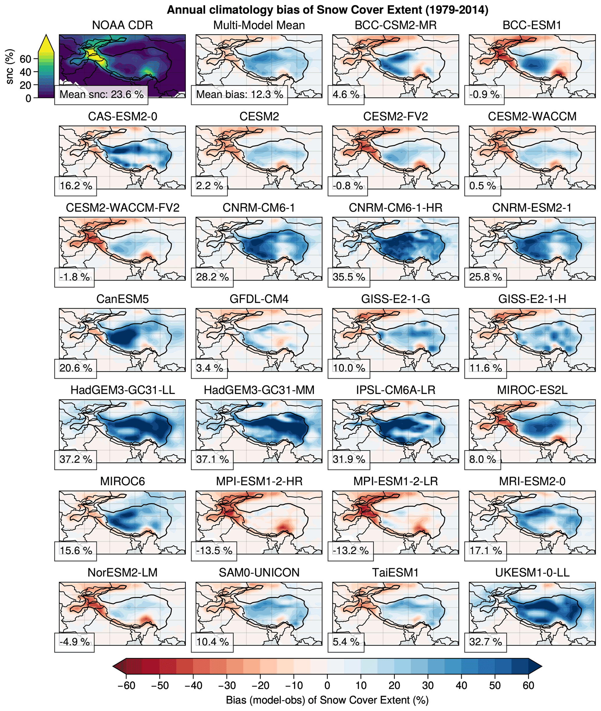
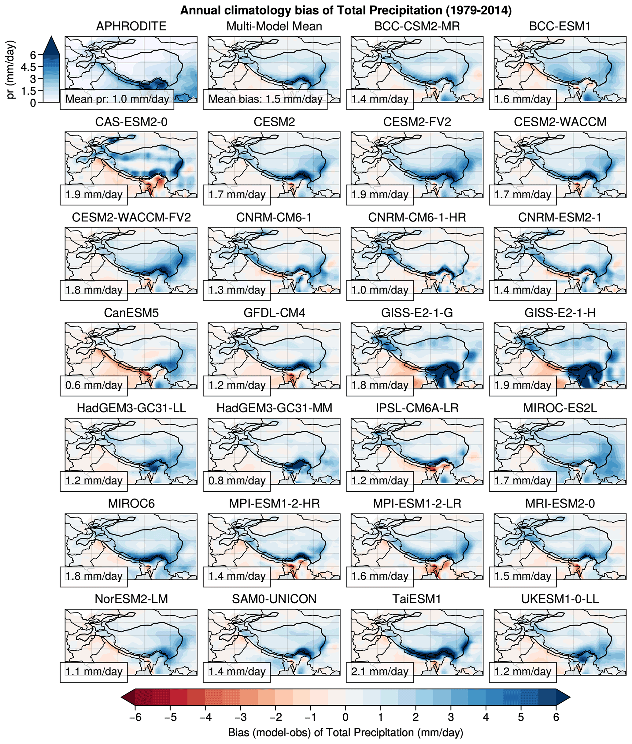
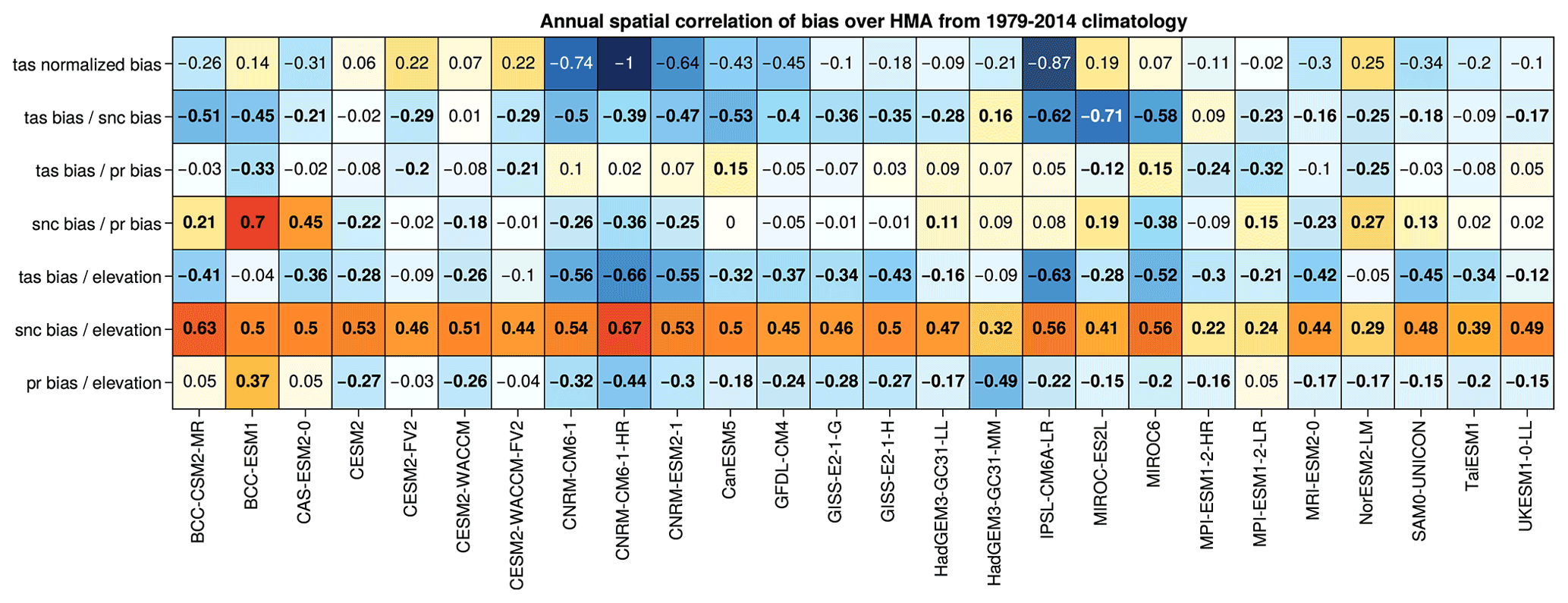
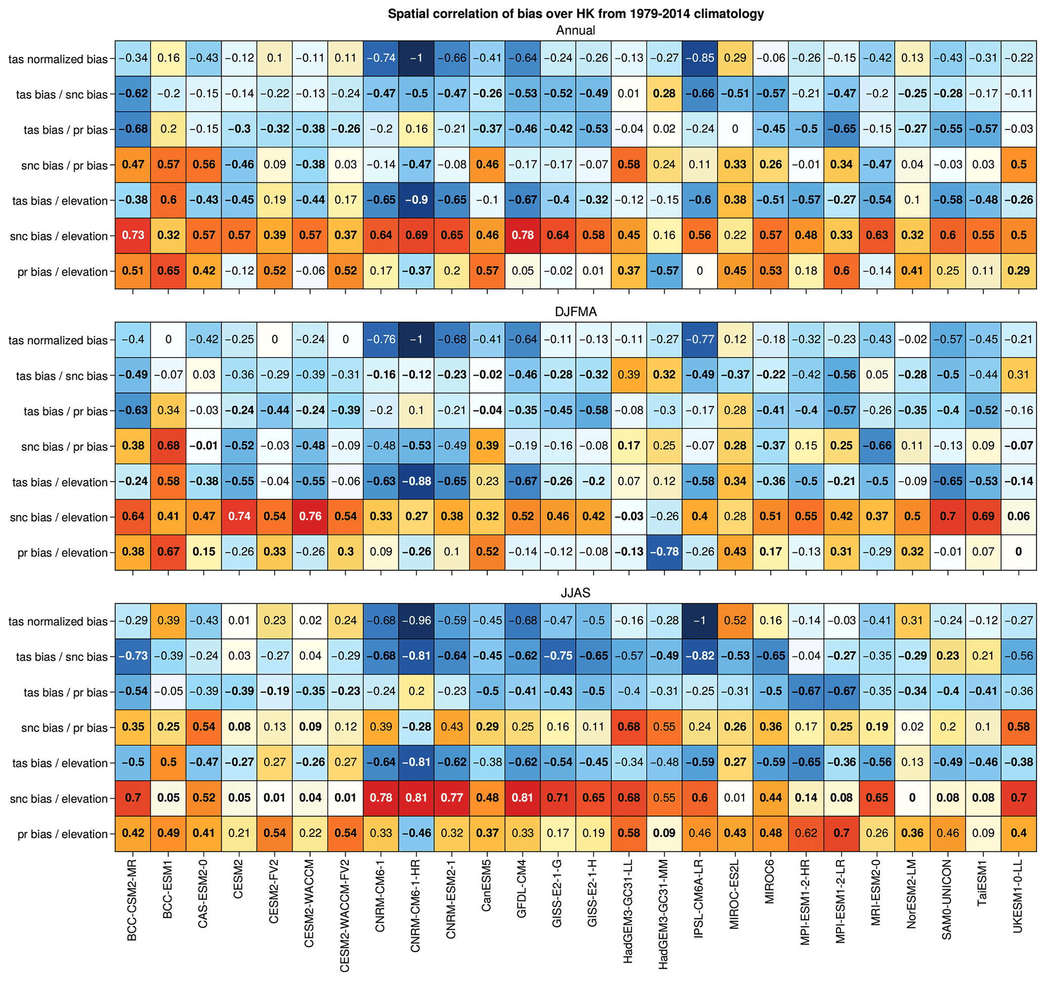
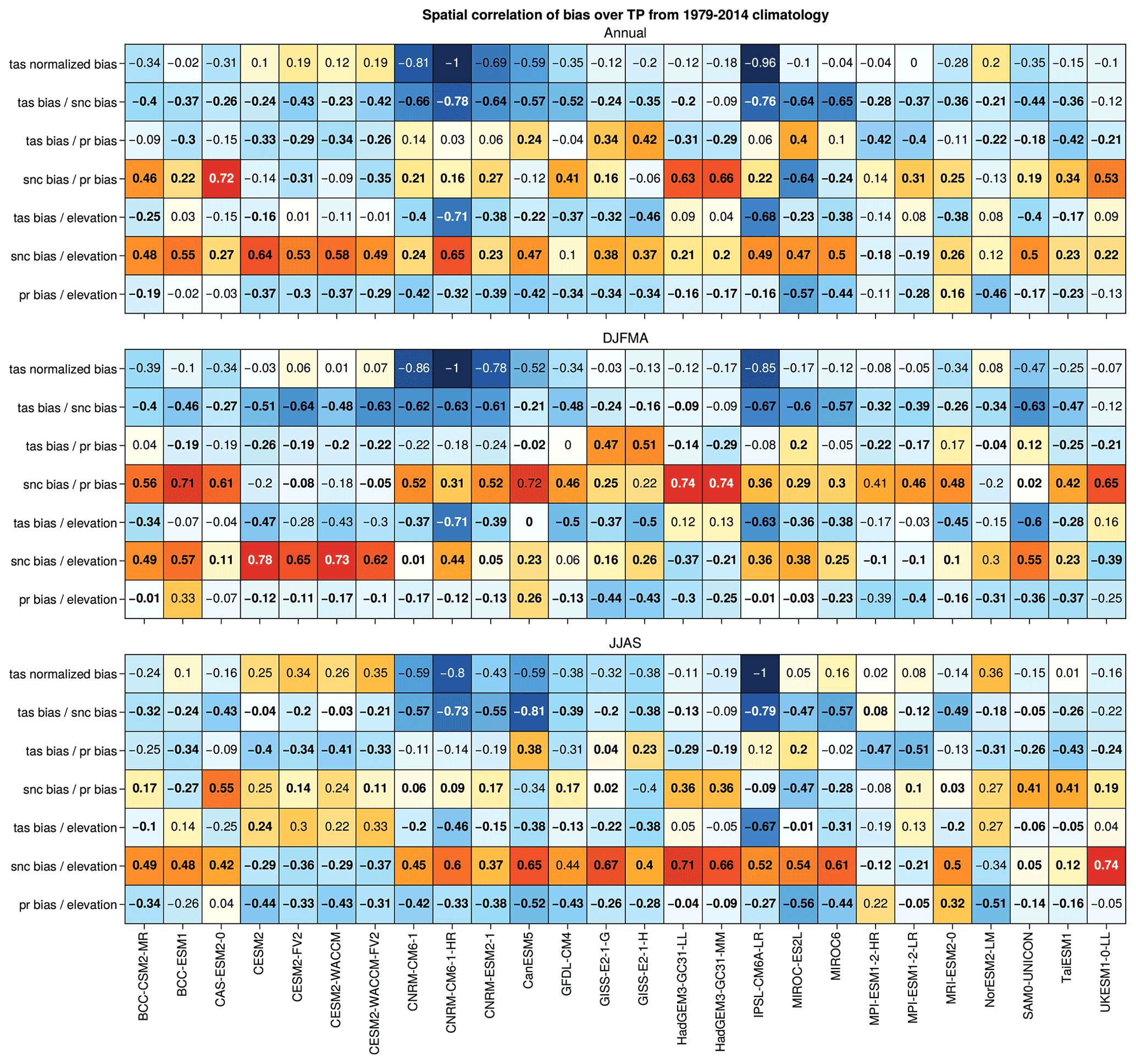
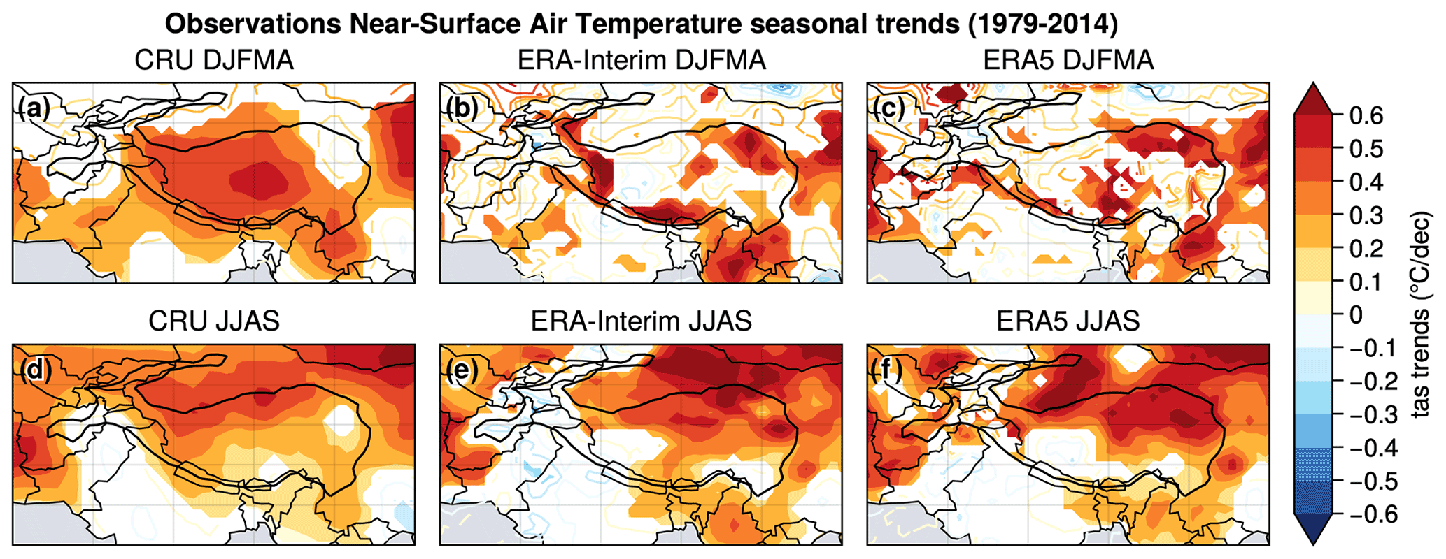
Figure D1Same as Fig. 7 but for observations and reanalyses comparison with only near-surface air temperature.

Figure D2Same as Fig. 7 but for observations and reanalyses comparison with only snow cover extent.
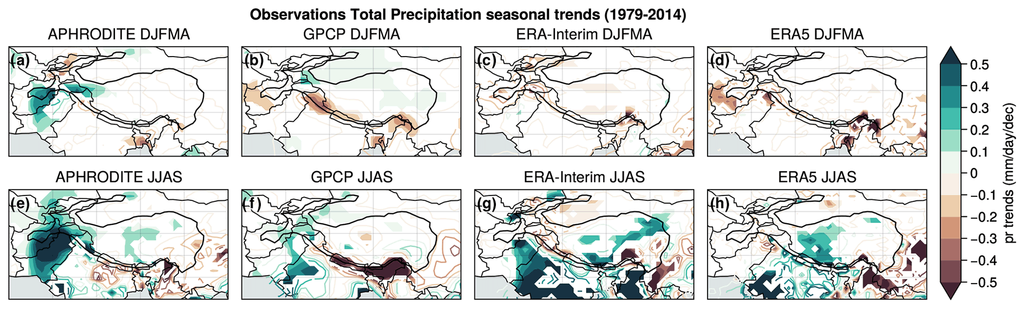
Figure D3Same as Fig. 7 but for observations and reanalyses comparison with only total precipitation.
Table E1Same as Table 2 but for relative anomalies only for snow cover and precipitation.
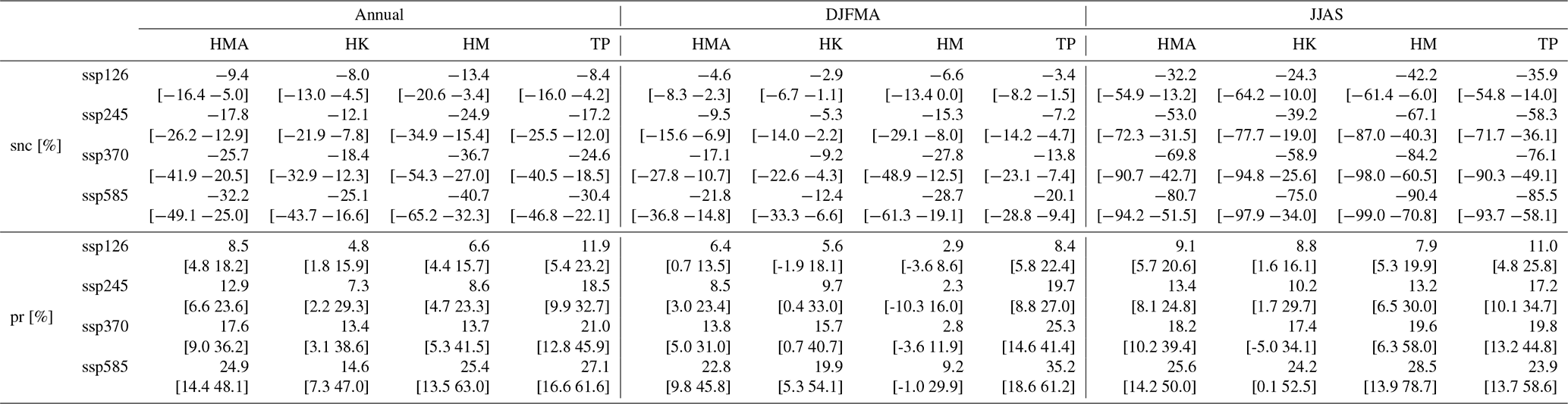
All scripts to produce the figures and results are available at https://github.com/mickaellalande/CMIP6_HMA_paper/tree/v1.0 (https://doi.org/10.5281/zenodo.5500285, Lalande, 2021). We use Python (Oliphant, 2007; Millman and Aivazis, 2011) version 3.8.5 and xarray (Hoyer and Hamman, 2017) version 0.16.0 to manipulate NetCDF files. Interpolations are performed using xESMF version 0.3.0 (https://doi.org/10.5281/zenodo.3700105, Zhuang et al., 2020a). For statistical purposes, Scipy (Virtanen et al., 2020) version 1.5.2 is used. All graphics are made using Proplot version 0.6.4 based on Matplotlib (Hunter, 2007) version 3.2.2 and Cartopy version 0.18.0. The Taylor diagrams were made thanks to the Python implementation of Yannick Copin (https://gist.github.com/ycopin/3342888; https://doi.org/10.5281/zenodo.5548061, Copin, 2012).
The datasets from CMIP6 simulations are available via the CMIP6 search interface: https://esgf-node.llnl.gov/search/cmip6/ (WCRP, 2021). CRU TS version 4.00 is available at https://doi.org/10.5285/edf8febfdaad48abb2cbaf7d7e846a86 (University of East Anglia Climatic Research Unit et al., 2017). NOAA CDR of NH snow cover extent version 1 is available at https://doi.org/10.7289/V5N014G9 (Robinson et al., 2012). The ESA CCI snow product is available at https://doi.org/10.5285/5484dc1392bc43c1ace73ba38a22ac56 (Naegeli et al., 2021), and the cloud gap filter used in this study can be provided upon request. The APHRODITE products are available here: http://aphrodite.st.hirosaki-u.ac.jp/download/ (APHRODITE's Water Resources, 2021). GPCP CDR version 2.3 (monthly) is available at https://doi.org/10.7289/V56971M6 (Adler et al., 2016). GMTED2010 can be found here: https://www.temis.nl/data/gmted2010/index.php (TEMIS, 2021). The GLDAS Land/Sea Mask Dataset at 1∘ can be found here: https://ldas.gsfc.nasa.gov/gldas/vegetation-class-mask (NASA, 2021). We also used the ERA-Interim and ERA5 reanalyses data that are publicly available at https://www.ecmwf.int/en/forecasts/datasets/reanalysis-datasets/era-interim (ECMWF, 2020b) and https://doi.org/10.24381/cds.adbb2d47 (Hersbach et al., 2018).
ML, MM and GK designed the study. ML produced the figures. ML and MM wrote the article and other authors contributed with suggested changes and comments. The ESA CCI snow products were provided by KN. All authors discussed the results and provided critical feedback.
The contact author has declared that neither they nor their co-authors have any competing interests.
Publisher’s note: Copernicus Publications remains neutral with regard to jurisdictional claims in published maps and institutional affiliations.
We acknowledge the World Climate Research Programme (WCRP), which, through its Working Group on Coupled Modelling, coordinated and promoted CMIP6. We thank the climate modeling groups for producing and making available their model output, the Earth System Grid Federation (ESGF) for archiving the data and providing access, and the multiple funding agencies who support CMIP6 and ESGF. We thank the CLIMERI-France infrastructure (http://climeri-france.fr/, last access: 5 October 2021) for making the CMIP6 data available. The authors thank the two anonymous reviewers for their constructive comments and their contribution to the improvement of this paper.
This research has been supported by the European Space Agency (ESA) Snow Climate Change Initiative (CCI+) project (grant no. 4000124098/18/I-NB).
This paper was edited by Govindasamy Bala and reviewed by two anonymous referees.
Adler, R., Wang, J.-J., Sapiano, M., Huffman, G., Chiu, L., Xie, P. P., Ferraro, R., Schneider, U., Becker, A., Bolvin, D., Nelkin, E., Gu, G., and CDR, P. N.: Global Precipitation Climatology Project (GPCP) Climate Data Record (CDR), Version 2.3 (Monthly), https://doi.org/10.7289/V56971M6, 2016. a, b
Adler, R., Sapiano, M., Huffman, G., Wang, J.-J., Gu, G., Bolvin, D., Chiu, L., Schneider, U., Becker, A., Nelkin, E., Xie, P., Ferraro, R., and Shin, D.-B.: The Global Precipitation Climatology Project (GPCP) Monthly Analysis (New Version 2.3) and a Review of 2017 Global Precipitation, Atmosphere, 9, 138, https://doi.org/10.3390/atmos9040138, 2018. a
APHRODITE's Water Resources: Download, available at: http://aphrodite.st.hirosaki-u.ac.jp/download/, last access: 14 June 2021. a
Bao, Y. and You, Q.: How do westerly jet streams regulate the winter snow depth over the Tibetan Plateau?, Clim. Dynam., 53, 353–370, https://doi.org/10.1007/s00382-018-4589-1, 2019. a
Bengtsson, L.: Can climate trends be calculated from reanalysis data?, J. Geophys. Res., 109, D11111, https://doi.org/10.1029/2004JD004536, 2004. a
Bookhagen, B. and Burbank, D. W.: Toward a complete Himalayan hydrological budget: Spatiotemporal distribution of snowmelt and rainfall and their impact on river discharge, J. Geophys. Res., 115, F03019, https://doi.org/10.1029/2009JF001426, 2010. a, b
Boos, W. R. and Hurley, J. V.: Thermodynamic Bias in the Multimodel Mean Boreal Summer Monsoon, J. Climate, 26, 2279–2287, https://doi.org/10.1175/JCLI-D-12-00493.1, 2013. a
Boos, W. R. and Kuang, Z.: Dominant control of the South Asian monsoon by orographic insulation versus plateau heating, Nature, 463, 218–222, https://doi.org/10.1038/nature08707, 2010. a
Bormann, K. J., Brown, R. D., Derksen, C., and Painter, T. H.: Estimating snow-cover trends from space, Nat. Clim. Change, 8, 924–928, https://doi.org/10.1038/s41558-018-0318-3, 2018. a, b
Boucher, O., Denvil, S., Levavasseur, G., Cozic, A., Caubel, A., Foujols, M.-A., Meurdesoif, Y., Cadule, P., Devilliers, M., Ghattas, J., Lebas, N., Lurton, T., Mellul, L., Musat, I., Mignot, J., and Cheruy, F.: IPSL IPSL-CM6A-LR model output prepared for CMIP6 CMIP historical, Version 20180803, Earth System Grid Federation [data set], https://doi.org/10.22033/ESGF/CMIP6.5195, 2018. a
Boucher, O., Denvil, S., Levavasseur, G., Cozic, A., Caubel, A., Foujols, M.-A., Meurdesoif, Y., Cadule, P., Devilliers, M., Dupont, E., and Lurton, T.: IPSL IPSL-CM6A-LR model output prepared for CMIP6 ScenarioMIP, Version 20190903, Earth System Grid Federation [data set], https://doi.org/10.22033/ESGF/CMIP6.1532, 2019. a
Brown, R. D. and Robinson, D. A.: Northern Hemisphere spring snow cover variability and change over 1922–2010 including an assessment of uncertainty, The Cryosphere, 5, 219–229, https://doi.org/10.5194/tc-5-219-2011, 2011. a
Brun, F., Berthier, E., Wagnon, P., Kääb, A., and Treichler, D.: A spatially resolved estimate of High Mountain Asia glacier mass balances from 2000 to 2016, Nat. Geosci., 10, 668–673, https://doi.org/10.1038/ngeo2999, 2017. a
Cannon, F., Carvalho, L. M. V., Jones, C., and Bookhagen, B.: Multi-annual variations in winter westerly disturbance activity affecting the Himalaya, Clim. Dynam., 44, 441–455, https://doi.org/10.1007/s00382-014-2248-8, 2015. a, b, c
Chai, Z.: CAS CAS-ESM1.0 model output prepared for CMIP6 CMIP historical, Version 20201227, Earth System Grid Federation [data set], https://doi.org/10.22033/ESGF/CMIP6.3353, 2020. a
Chen, X., Liu, Y., and Wu, G.: Understanding the surface temperature cold bias in CMIP5 AGCMs over the Tibetan Plateau, Adv. Atmos. Sci., 34, 1447–1460, https://doi.org/10.1007/s00376-017-6326-9, 2017. a, b, c, d, e
Cheruy, F., Ducharne, A., Hourdin, F., Musat, I., Vignon, é., Gastineau, G., Bastrikov, V., Vuichard, N., Diallo, B., Dufresne, J., Ghattas, J., Grandpeix, J., Idelkadi, A., Mellul, L., Maignan, F., Ménégoz, M., Ottlé, C., Peylin, P., Servonnat, J., Wang, F., and Zhao, Y.: Improved Near‐Surface Continental Climate in IPSL‐CM6A‐LR by Combined Evolutions of Atmospheric and Land Surface Physics, J. Adv. Model. Earth Sy., 12, e2019MS002005, https://doi.org/10.1029/2019MS002005, 2020. a
Copin, Y.: Taylor diagram for python/matplotlib (2018-12-06), Zenodo [code], https://doi.org/10.5281/zenodo.5548061, 2012. a
Dahe, Q., Shiyin, L., and Peiji, L.: Snow Cover Distribution, Variability, and Response to Climate Change in Western China, J. Climate, 19, 1820–1833, https://doi.org/10.1175/JCLI3694.1, 2006. a
Danabasoglu, G.: NCAR CESM2 model output prepared for CMIP6 CMIP historical, Version 20190308, Earth System Grid Federation [data set], https://doi.org/10.22033/ESGF/CMIP6.7627 2019a. a
Danabasoglu, G.: NCAR CESM2-FV2 model output prepared for CMIP6 CMIP historical, Version 20191120, Earth System Grid Federation [data set], https://doi.org/10.22033/ESGF/CMIP6.11297, 2019b. a
Danabasoglu, G.: NCAR CESM2-WACCM model output prepared for CMIP6 CMIP historical, Version 20190227, Earth System Grid Federation [data set], https://doi.org/10.22033/ESGF/CMIP6.10071, 2019c. a
Danabasoglu, G.: NCAR CESM2-WACCM-FV2 model output prepared for CMIP6 CMIP historical, Version 20191120, Earth System Grid Federation [data set], https://doi.org/10.22033/ESGF/CMIP6.11298, 2019d. a
Danielson, J. and Gesch, D.: Global Multi-resolution Terrain Elevation Data 2010 (GMTED2010), U.S. Geological Survey Open-File Report 2011–1073, 2010, 26, available at: http://pubs.usgs.gov/of/2011/1073/pdf/of2011-1073.pdf (last access: 14 January 2021), 2011. a
Das, S., Giorgi, F., Giuliani, G., Dey, S., and Coppola, E.: Near‐Future Anthropogenic Aerosol Emission Scenarios and Their Direct Radiative Effects on the Present‐Day Characteristics of the Indian Summer Monsoon, J. Geophys. Res.-Atmos., 125, 1–19, https://doi.org/10.1029/2019JD031414, 2020. a
Dee, D. P., Uppala, S. M., Simmons, A. J., Berrisford, P., Poli, P., Kobayashi, S., Andrae, U., Balmaseda, M. A., Balsamo, G., Bauer, P., Bechtold, P., Beljaars, A. C. M., van de Berg, L., Bidlot, J., Bormann, N., Delsol, C., Dragani, R., Fuentes, M., Geer, A. J., Haimberger, L., Healy, S. B., Hersbach, H., Hólm, E. V., Isaksen, L., Kållberg, P., Köhler, M., Matricardi, M., McNally, A. P., Monge-Sanz, B. M., Morcrette, J.-J., Park, B.-K., Peubey, C., de Rosnay, P., Tavolato, C., Thépaut, J.-N., and Vitart, F.: The ERA-Interim reanalysis: configuration and performance of the data assimilation system, Q. J. Roy. Meteor. Soc., 137, 553–597, https://doi.org/10.1002/qj.828, 2011. a
Déry, S. J. and Brown, R. D.: Recent Northern Hemisphere snow cover extent trends and implications for the snow-albedo feedback, Geophys. Res. Lett., 34, L22504, https://doi.org/10.1029/2007GL031474, 2007. a
Deser, C., Lehner, F., Rodgers, K. B., Ault, T., Delworth, T. L., DiNezio, P. N., Fiore, A., Frankignoul, C., Fyfe, J. C., Horton, D. E., Kay, J. E., Knutti, R., Lovenduski, N. S., Marotzke, J., McKinnon, K. A., Minobe, S., Randerson, J., Screen, J. A., Simpson, I. R., and Ting, M.: Insights from Earth system model initial-condition large ensembles and future prospects, Nat. Clim. Change, 10, 277–286, https://doi.org/10.1038/s41558-020-0731-2, 2020. a
Devasthale, A., Raspaud, M., Schlundt, C., Hanschmann, T., Finkensieper, S., Dybbroe, A., Hörnquist, S., Håkansson, N., Stengel, M., and Karlsson, K.-G.: PyGAC: An open-source, community-driven Python interface to preprocess nearly 40-year AVHRR Global Area Coverage (GAC) datarecord, GSICS Quartherly Newsl., 11, 3–5, https://doi.org/10.7289/V5R78CFR, 2017. a
De Wekker, S. F. J. and Kossmann, M.: Convective Boundary Layer Heights Over Mountainous Terrain – A Review of Concepts, Front. Earth Sci., 3, 1–22, https://doi.org/10.3389/feart.2015.00077, 2015. a
Dimri, A., Yasunari, T., Wiltshire, A., Kumar, P., Mathison, C., Ridley, J., and Jacob, D.: Application of regional climate models to the Indian winter monsoon over the western Himalayas, Sci. Total Environ., 468–469, S36–S47, https://doi.org/10.1016/j.scitotenv.2013.01.040, 2013. a
Ding, J., Cuo, L., Zhang, Y., and Zhu, F.: Monthly and annual temperature extremes and their changes on the Tibetan Plateau and its surroundings during 1963–2015, Sci. Rep.-UK, 8, 1–23, https://doi.org/10.1038/s41598-018-30320-0, 2018. a
Drusch, M., Vasiljevic, D., and Viterbo, P.: ECMWF's Global Snow Analysis: Assessment and Revision Based on Satellite Observations, J. Appl. Meteorol., 43, 1282–1294, https://doi.org/10.1175/1520-0450(2004)043<1282:EGSAAA>2.0.CO;2, 2004. a, b, c
Du, Z. and Qingsong, Z.: Introduction, in: Mountain Geoecology and Sustainable Development of the Tibetan Plateau, chap. 1, Springer, Dordrecht, 1–17, https://doi.org/10.1007/978-94-010-0965-2_1, 2000. a
Duan, A., Hu, J., and Xiao, Z.: The Tibetan Plateau Summer Monsoon in the CMIP5 Simulations, J. Climate, 26, 7747–7766, https://doi.org/10.1175/JCLI-D-12-00685.1, 2013. a
Duan, A. M. and Wu, G. X.: Role of the Tibetan Plateau thermal forcing in the summer climate patterns over subtropical Asia, Clim. Dynam., 24, 793–807, https://doi.org/10.1007/s00382-004-0488-8, 2005. a
ECMWF: IFS Documentation CY47R1 – Part II: Data Assimilation, in: IFS Documentation CY47R1, no. 2 in IFS Documentation, chap. 9.3.3, ECMWF, https://doi.org/10.21957/0gtybbwp9, 2020a. a
ECMWF: ERA-Interim, available at: https://www.ecmwf.int/en/forecasts/datasets/reanalysis-datasets/era-interim, last access: 6 October 2020b. a
Estilow, T. W., Young, A. H., and Robinson, D. A.: A long-term Northern Hemisphere snow cover extent data record for climate studies and monitoring, Earth Syst. Sci. Data, 7, 137–142, https://doi.org/10.5194/essd-7-137-2015, 2015. a
Eyring, V., Bony, S., Meehl, G. A., Senior, C. A., Stevens, B., Stouffer, R. J., and Taylor, K. E.: Overview of the Coupled Model Intercomparison Project Phase 6 (CMIP6) experimental design and organization, Geosci. Model Dev., 9, 1937–1958, https://doi.org/10.5194/gmd-9-1937-2016, 2016. a, b
Flohn, H.: Large-scale Aspects of the “Summer Monsoon” in South and East Asia, J. Meteorol. Soc. Jpn., 35, 180–186, https://doi.org/10.2151/jmsj1923.35A.0_180, 1957. a
Foppa, N. and Seiz, G.: Inter-annual variations of snow days over Switzerland from 2000–2010 derived from MODIS satellite data, The Cryosphere, 6, 331–342, https://doi.org/10.5194/tc-6-331-2012, 2012. a
Forster, P. M., Maycock, A. C., McKenna, C. M., and Smith, C. J.: Latest climate models confirm need for urgent mitigation, Nat. Clim. Change, 10, 7–10, https://doi.org/10.1038/s41558-019-0660-0, 2020. a
Gao, L., Hao, L., and Chen, X.-w.: Evaluation of ERA-interim monthly temperature data over the Tibetan Plateau, J. Mt. Sci., 11, 1154–1168, https://doi.org/10.1007/s11629-014-3013-5, 2014. a
Good, P., Sellar, A., Tang, Y., Rumbold, S., Ellis, R., Kelley, D., Kuhlbrodt, T., and Walton, J.: MOHC UKESM1.0-LL model output prepared for CMIP6 ScenarioMIP, Version 20190503, Earth System Grid Federation [data set], https://doi.org/10.22033/ESGF/CMIP6.1567, 2019. a
Grohmann, C. H.: COMPARATIVE ANALYSIS OF GLOBAL DIGITAL ELEVATION MODELS AND ULTRA-PROMINENT MOUNTAIN PEAKS, ISPRS Annals of Photogrammetry, Remote Sensing and Spatial Information Sciences, III-4, 17–23, https://doi.org/10.5194/isprsannals-III-4-17-2016, 2016. a
Gu, H., Wang, G., Yu, Z., and Mei, R.: Assessing future climate changes and extreme indicators in east and south Asia using the RegCM4 regional climate model, Climatic Change, 114, 301–317, https://doi.org/10.1007/s10584-012-0411-y, 2012. a, b, c, d
Guo, H., John, J. G., Blanton, C., McHugh, C., Nikonov, S., Radhakrishnan, A., Rand, K., Zadeh, N. T., Balaji, V., Durachta, J., Dupuis, C., Menzel, R., Robinson, T., Underwood, S., Vahlenkamp, H., Bushuk, M., Dunne, K. A., Dussin, R., Gauthier, P. P. G., Ginoux, P., Griffies, S. M., Hallberg, R., Harrison, M., Hurlin, W., Lin, P., Malyshev, S., Naik, V., Paulot, F., Paynter, D. J., Ploshay, J., Reichl, B. G., Schwarzkopf, D. M., Seman, C. J., Shao, A., Silvers, L., Wyman, B., Yan, X., Zeng, Y., Adcroft, A., Dunne, J. P., Held, I. M., Krasting, J. P., Horowitz, L. W., Milly, P. C. D., Shevliakova, E., Winton, M., Zhao, M., and Zhang, R.: NOAA-GFDL GFDL-CM4 model output historical, Version 20180701, Earth System Grid Federation [data set], https://doi.org/10.22033/ESGF/CMIP6.8594, 2018. a
Gurung, D. R., Maharjan, S. B., Shrestha, A. B., Shrestha, M. S., Bajracharya, S. R., and Murthy, M. S. R.: Climate and topographic controls on snow cover dynamics in the Hindu Kush Himalaya, Int. J. Climatol., 37, 3873–3882, https://doi.org/10.1002/joc.4961, 2017. a
Harris, I., Osborn, T. J., Jones, P., and Lister, D.: Version 4 of the CRU TS monthly high-resolution gridded multivariate climate dataset, Scientific Data, 7, 109, https://doi.org/10.1038/s41597-020-0453-3, 2020. a
Hajima, T., Abe, M., Arakawa, O., Suzuki, T., Komuro, Y., Ogura, T., Ogochi, K., Watanabe, M., Yamamoto, A., Tatebe, H., Noguchi, M. A., Ohgaito, R., Ito, A., Yamazaki, D., Ito, A., Takata, K., Watanabe, S., Kawamiya, M., and Tachiiri, K.: MIROC MIROC-ES2L model output prepared for CMIP6 CMIP historical, Version 20190823, Earth System Grid Federation [data set], https://doi.org/10.22033/ESGF/CMIP6.5602, 2019. a
Hawkins, E., Smith, R. S., Gregory, J. M., and Stainforth, D. A.: Irreducible uncertainty in near-term climate projections, Clim. Dynam., 46, 3807–3819, https://doi.org/10.1007/s00382-015-2806-8, 2016. a, b
Helfrich, S. R., McNamara, D., Ramsay, B. H., Baldwin, T., and Kasheta, T.: Enhancements to, and forthcoming developments in the Interactive Multisensor Snow and Ice Mapping System (IMS), Hydrol. Process., 21, 1576–1586, https://doi.org/10.1002/hyp.6720, 2007. a, b
Hernández-Henríquez, M. A., Déry, S. J., and Derksen, C.: Polar amplification and elevation-dependence in trends of Northern Hemisphere snow cover extent, 1971–2014, Environ. Res. Lett., 10, 044010, https://doi.org/10.1088/1748-9326/10/4/044010, 2015. a
Hersbach, H., Bell, B., Berrisford, P., Biavati, G., Horányi, A., Muñoz Sabater, J., Nicolas, J., Peubey, C., Radu, R., Rozum, I., Schepers, D., Simmons, A., Soci, C., Dee, D., and Thépaut, J.-N.: ERA5 hourly data on single levels from 1979 to present, Copernicus Climate Change Service (C3S) Climate Data Store (CDS) [data set], https://doi.org/10.24381/cds.adbb2d47, 2018. a
Hersbach, H., Bell, B., Berrisford, P., Hirahara, S., Horányi, A., Muñoz‐Sabater, J., Nicolas, J., Peubey, C., Radu, R., Schepers, D., Simmons, A., Soci, C., Abdalla, S., Abellan, X., Balsamo, G., Bechtold, P., Biavati, G., Bidlot, J., Bonavita, M., Chiara, G., Dahlgren, P., Dee, D., Diamantakis, M., Dragani, R., Flemming, J., Forbes, R., Fuentes, M., Geer, A., Haimberger, L., Healy, S., Hogan, R. J., Hólm, E., Janisková, M., Keeley, S., Laloyaux, P., Lopez, P., Lupu, C., Radnoti, G., Rosnay, P., Rozum, I., Vamborg, F., Villaume, S., and Thépaut, J.: The ERA5 global reanalysis, Q. J. Roy. Meteor. Soc., 146, 1999–2049, https://doi.org/10.1002/qj.3803, 2020. a, b, c
Hori, M., Sugiura, K., Kobayashi, K., Aoki, T., Tanikawa, T., Kuchiki, K., Niwano, M., and Enomoto, H.: A 38-year (1978–2015) Northern Hemisphere daily snow cover extent product derived using consistent objective criteria from satellite-borne optical sensors, Remote Sens. Environ., 191, 402–418, https://doi.org/10.1016/j.rse.2017.01.023, 2017. a
Hoyer, S. and Hamman, J. J.: xarray: N-D labeled Arrays and Datasets in Python, Journal of Open Research Software, 5, 1–6, https://doi.org/10.5334/jors.148, 2017. a
Hsu, H. and Liu, X.: Relationship between the Tibetan Plateau heating and East Asian summer monsoon rainfall, Geophys. Res. Lett., 30, 2003GL017909, https://doi.org/10.1029/2003GL017909, 2003. a
Hunt, K. M. R., Turner, A. G., and Shaffrey, L. C.: The evolution, seasonality and impacts of western disturbances, Q. J. Roy. Meteor. Soc., 144, 278–290, https://doi.org/10.1002/qj.3200, 2018. a, b
Hunter, J. D.: Matplotlib: A 2D Graphics Environment, Comput. Sci. Eng., 9, 90–95, https://doi.org/10.1109/MCSE.2007.55, 2007. a
Immerzeel, W., Droogers, P., de Jong, S., and Bierkens, M.: Large-scale monitoring of snow cover and runoff simulation in Himalayan river basins using remote sensing, Remote Sens. Environ., 113, 40–49, https://doi.org/10.1016/j.rse.2008.08.010, 2009. a
Immerzeel, W. W. and Bierkens, M. F. P.: Asia's water balance, Nat. Geosci., 5, 841–842, https://doi.org/10.1038/ngeo1643, 2012. a
Immerzeel, W. W., van Beek, L. P. H., and Bierkens, M. F. P.: Climate Change Will Affect the Asian Water Towers, Science, 328, 1382–1385, https://doi.org/10.1126/science.1183188, 2010. a, b
Immerzeel, W. W., Wanders, N., Lutz, A. F., Shea, J. M., and Bierkens, M. F. P.: Reconciling high-altitude precipitation in the upper Indus basin with glacier mass balances and runoff, Hydrol. Earth Syst. Sci., 19, 4673–4687, https://doi.org/10.5194/hess-19-4673-2015, 2015. a, b
Jimeno-Sáez, P., Pulido-Velazquez, D., Collados-Lara, A.-J., Pardo-Igúzquiza, E., Senent-Aparicio, J., and Baena-Ruiz, L.: A Preliminary Assessment of the “Undercatching” and the Precipitation Pattern in an Alpine Basin, Water, 12, 1061, https://doi.org/10.3390/w12041061, 2020. a
Jungclaus, J., Bittner, M., Wieners, K.-H., Wachsmann, F., Schupfner, M., Legutke, S., Giorgetta, M., Reick, C., Gayler, V., Haak, H., de Vrese, P., Raddatz, T., Esch, M., Mauritsen, T., von Storch, J.-S., Behrens, J., Brovkin, V., Claussen, M., Crueger, T., Fast, I., Fiedler, S., Hagemann, S., Hohenegger, C., Jahns, T., Kloster, S., Kinne, S., Lasslop, G., Kornblueh, L., Marotzke, J., Matei, D., Meraner, K., Mikolajewicz, U., Modali, K., Müller, W., Nabel, J., Notz, D., Peters-von Gehlen, K., Pincus, R., Pohlmann, H., Pongratz, J., Rast, S., Schmidt, H., Schnur, R., Schulzweida, U., Six, K., Stevens, B., Voigt, A., and Roeckner, E.: MPI-M MPI-ESM1.2-HR model output prepared for CMIP6 CMIP historical, Version 20190710, Earth System Grid Federation [data set], https://doi.org/10.22033/ESGF/CMIP6.6594, 2019. a
Kang, S., Xu, Y., You, Q., Flügel, W.-A., Pepin, N., and Yao, T.: Review of climate and cryospheric change in the Tibetan Plateau, Environ. Res. Lett., 5, 015101, https://doi.org/10.1088/1748-9326/5/1/015101, 2010. a
Kapnick, S. B., Delworth, T. L., Ashfaq, M., Malyshev, S., and Milly, P. C. D.: Snowfall less sensitive to warming in Karakoram than in Himalayas due to a unique seasonal cycle, Nat. Geosci., 7, 834–840, https://doi.org/10.1038/ngeo2269, 2014. a, b, c, d
Katzenberger, A., Schewe, J., Pongratz, J., and Levermann, A.: Robust increase of Indian monsoon rainfall and its variability under future warming in CMIP6 models, Earth Syst. Dynam., 12, 367–386, https://doi.org/10.5194/esd-12-367-2021, 2021. a
Knutti, R., Furrer, R., Tebaldi, C., Cermak, J., and Meehl, G. A.: Challenges in Combining Projections from Multiple Climate Models, J. Climate, 23, 2739–2758, https://doi.org/10.1175/2009JCLI3361.1, 2010. a
Krinner, G., Kharin, V., Roehrig, R., Scinocca, J., and Codron, F.: Historically-based run-time bias corrections substantially improve model projections of 100 years of future climate change, Communications Earth & Environment, 1, 29, https://doi.org/10.1038/s43247-020-00035-0, 2020. a
Krishnan, R., Sabin, T. P., Ayantika, D. C., Kitoh, A., Sugi, M., Murakami, H., Turner, A. G., Slingo, J. M., and Rajendran, K.: Will the South Asian monsoon overturning circulation stabilize any further?, Clim. Dynam., 40, 187–211, https://doi.org/10.1007/s00382-012-1317-0, 2013. a
Krishnan, R., Sabin, T. P., Vellore, R., Mujumdar, M., Sanjay, J., Goswami, B. N., Hourdin, F., Dufresne, J.-L., and Terray, P.: Deciphering the desiccation trend of the South Asian monsoon hydroclimate in a warming world, Clim. Dynam., 47, 1007–1027, https://doi.org/10.1007/s00382-015-2886-5, 2016. a
Krishnan, R., Sabin, T. P., Madhura, R. K., Vellore, R. K., Mujumdar, M., Sanjay, J., Nayak, S., and Rajeevan, M.: Non-monsoonal precipitation response over the Western Himalayas to climate change, Clim. Dynam., 52, 4091–4109, https://doi.org/10.1007/s00382-018-4357-2, 2019. a, b, c, d
Kutzbach, J. E., Prell, W. L., and Ruddiman, W. F.: Sensitivity of Eurasian Climate to Surface Uplift of the Tibetan Plateau, J. Geol., 101, 177–190, https://doi.org/10.1086/648215, 1993. a
Lalande, M.: mickaellalande/CMIP6_HMA_paper: First release for production in ESD (v1.0), Zenodo [code], https://doi.org/10.5281/zenodo.5500285, 2021. a
Lee, W.-L. and Liang, H.-C.: AS-RCEC TaiESM1.0 model output prepared for CMIP6 CMIP historical, Version 20200623, Earth System Grid Federation [data set], https://doi.org/10.22033/ESGF/CMIP6.9755, 2020. a
Lee, D.-K. and Suh, M.-S.: Ten-year east Asian summer monsoon simulation using a regional climate model (RegCM2), J. Geophys. Res.-Atmos., 105, 29565–29577, https://doi.org/10.1029/2000JD900438, 2000. a
Li, C. and Yanai, M.: The Onset and Interannual Variability of the Asian Summer Monsoon in Relation to Land–Sea Thermal Contrast, J. Climate, 9, 358–375, https://doi.org/10.1175/1520-0442(1996)009<0358:TOAIVO>2.0.CO;2, 1996. a
Li, C., Su, F., Yang, D., Tong, K., Meng, F., and Kan, B.: Spatiotemporal variation of snow cover over the Tibetan Plateau based on MODIS snow product, 2001–2014, Int. J. Climatol., 38, 708–728, https://doi.org/10.1002/joc.5204, 2018. a, b
Lin, C., Chen, D., Yang, K., and Ou, T.: Impact of model resolution on simulating the water vapor transport through the central Himalayas: implication for models’ wet bias over the Tibetan Plateau, Clim. Dynam., 51, 3195–3207, https://doi.org/10.1007/s00382-018-4074-x, 2018. a
Liu, X. and Chen, B.: Climatic warming in the Tibetan Plateau during recent decades, International Journal of Climatology, 20, 1729–1742, https://doi.org/10.1002/1097-0088(20001130)20:14<1729::AID-JOC556>3.0.CO;2-Y, 2000. a, b
Liu, Y., Bao, Q., Duan, A., Qian, Z., and Wu, G.: Recent progress in the impact of the Tibetan Plateau on climate in China, Adv. Atmos. Sci., 24, 1060–1076, https://doi.org/10.1007/s00376-007-1060-3, 2007. a
Madhura, R. K., Krishnan, R., Revadekar, J. V., Mujumdar, M., and Goswami, B. N.: Changes in western disturbances over the Western Himalayas in a warming environment, Clim. Dynam., 44, 1157–1168, https://doi.org/10.1007/s00382-014-2166-9, 2015. a
Mao, J. and Robock, A.: Surface Air Temperature Simulations by AMIP General Circulation Models: Volcanic and ENSO Signals and Systematic Errors, J. Climate, 11, 1538–1552, https://doi.org/10.1175/1520-0442(1998)011<1538:SATSBA>2.0.CO;2, 1998. a, b
Meehl, G. A., Senior, C. A., Eyring, V., Flato, G., Lamarque, J.-F., Stouffer, R. J., Taylor, K. E., and Schlund, M.: Context for interpreting equilibrium climate sensitivity and transient climate response from the CMIP6 Earth system models, Science Advances, 6, eaba1981, https://doi.org/10.1126/sciadv.aba1981, 2020. a
Ménégoz, M., Krinner, G., Balkanski, Y., Boucher, O., Cozic, A., Lim, S., Ginot, P., Laj, P., Gallée, H., Wagnon, P., Marinoni, A., and Jacobi, H. W.: Snow cover sensitivity to black carbon deposition in the Himalayas: from atmospheric and ice core measurements to regional climate simulations, Atmos. Chem. Phys., 14, 4237–4249, https://doi.org/10.5194/acp-14-4237-2014, 2014. a
Metsämäki, S., Pulliainen, J., Salminen, M., Luojus, K., Wiesmann, A., Solberg, R., Böttcher, K., Hiltunen, M., and Ripper, E.: Introduction to GlobSnow Snow Extent products with considerations for accuracy assessment, Remote Sens. Environ., 156, 96–108, https://doi.org/10.1016/j.rse.2014.09.018, 2015. a
Millman, K. J. and Aivazis, M.: Python for Scientists and Engineers, Comput. Sci. Eng., 13, 9–12, https://doi.org/10.1109/MCSE.2011.36, 2011. a
Mudryk, L., Santolaria-Otín, M., Krinner, G., Ménégoz, M., Derksen, C., Brutel-Vuilmet, C., Brady, M., and Essery, R.: Historical Northern Hemisphere snow cover trends and projected changes in the CMIP6 multi-model ensemble, The Cryosphere, 14, 2495–2514, https://doi.org/10.5194/tc-14-2495-2020, 2020. a, b
Naegeli, K., Neuhaus, C., Salberg, A.-B., Schwaizer, G., Wiesmann, A., Wunderle, S., and Nagler, T.: ESA Snow Climate Change Initiative (Snow_cci): Daily global Snow Cover Fraction – snow on ground (SCFG) from AVHRR (1982–2019), version1.0, 12 May 2021, NERC EDS Centre for Environmental Data Analysis [data set] https://doi.org/10.5285/5484dc1392bc43c1ace73ba38a22ac56, 2021. a, b
NASA: GLDAS Vegetation Class/Mask, available at: https://ldas.gsfc.nasa.gov/gldas/vegetation-class-mask, last access: 1 June 2021. a
NASA Goddard Institute for Space Studies (NASA/GISS): NASA-GISS GISS-E2.1G model output prepared for CMIP6 CMIP historical, Version 20180827, Earth System Grid Federation [data set], https://doi.org/10.22033/ESGF/CMIP6.7127, 2018. a
NASA Goddard Institute for Space Studies (NASA/GISS): NASA-GISS GISS-E2.1H model output prepared for CMIP6 CMIP historical, Version 20190403, Earth System Grid Federation [data set], https://doi.org/10.22033/ESGF/CMIP6.7128, 2019. a
Norris, J., Carvalho, L. M. V., Jones, C., and Cannon, F.: WRF simulations of two extreme snowfall events associated with contrasting extratropical cyclones over the western and central Himalaya, J. Geophys. Res.-Atmos., 120, 3114–3138, https://doi.org/10.1002/2014JD022592, 2015. a
Norris, J., Carvalho, L. M. V., Jones, C., Cannon, F., Bookhagen, B., Palazzi, E., and Tahir, A. A.: The spatiotemporal variability of precipitation over the Himalaya: evaluation of one-year WRF model simulation, Clim. Dynam., 49, 2179–2204, https://doi.org/10.1007/s00382-016-3414-y, 2017. a
Notarnicola, C.: Observing Snow Cover and Water Resource Changes in the High Mountain Asia Region in Comparison with Global Mountain Trends over 2000–2018, Remote Sensing, 12, 3913, https://doi.org/10.3390/rs12233913, 2020. a, b
Oliphant, T. E.: Python for Scientific Computing, Comput. Sci. Eng., 9, 10–20, https://doi.org/10.1109/MCSE.2007.58, 2007. a
O'Neill, B. C., Tebaldi, C., van Vuuren, D. P., Eyring, V., Friedlingstein, P., Hurtt, G., Knutti, R., Kriegler, E., Lamarque, J.-F., Lowe, J., Meehl, G. A., Moss, R., Riahi, K., and Sanderson, B. M.: The Scenario Model Intercomparison Project (ScenarioMIP) for CMIP6, Geosci. Model Dev., 9, 3461–3482, https://doi.org/10.5194/gmd-9-3461-2016, 2016. a, b
Orsolini, Y., Wegmann, M., Dutra, E., Liu, B., Balsamo, G., Yang, K., de Rosnay, P., Zhu, C., Wang, W., Senan, R., and Arduini, G.: Evaluation of snow depth and snow cover over the Tibetan Plateau in global reanalyses using in situ and satellite remote sensing observations, The Cryosphere, 13, 2221–2239, https://doi.org/10.5194/tc-13-2221-2019, 2019. a, b, c
Sabin, T. P., Krishnan, R., Ghattas, J., Denvil, S., Dufresne, J.-L., Hourdin, F., and Pascal, T.: High resolution simulation of the South Asian monsoon using a variable resolution global climate model, Clim. Dynam., 41, 173–194, https://doi.org/10.1007/s00382-012-1658-8, 2013. a
Palazzi, E., von Hardenberg, J., and Provenzale, A.: Precipitation in the Hindu-Kush Karakoram Himalaya: Observations and future scenarios, J. Geophys. Res.-Atmos., 118, 85–100, https://doi.org/10.1029/2012JD018697, 2013. a, b, c, d, e, f, g, h, i, j, k, l, m, n
Park, S. and Shin, J.: SNU SAM0-UNICON model output prepared for CMIP6 CMIP historical, Version 20190323, Earth System Grid Federation [data set], https://doi.org/10.22033/ESGF/CMIP6.7789, 2019. a
Pu, Z., Xu, L., and Salomonson, V. V.: MODIS/Terra observed seasonal variations of snow cover over the Tibetan Plateau, Geophys. Res. Lett., 34, L06706, https://doi.org/10.1029/2007GL029262, 2007. a
Qiu, J.: China: The third pole, Nature, 454, 393–396, https://doi.org/10.1038/454393a, 2008. a, b
Rangwala, I., Sinsky, E., and Miller, J. R.: Amplified warming projections for high altitude regions of the northern hemisphere mid-latitudes from CMIP5 models, Environ. Res. Lett., 8, 024040, https://doi.org/10.1088/1748-9326/8/2/024040, 2013. a
Rasul, G.: Food, water, and energy security in South Asia: A nexus perspective from the Hindu Kush Himalayan region☆, Environ. Sci. Policy, 39, 35–48, https://doi.org/10.1016/j.envsci.2014.01.010, 2014. a
Ridley, J., Menary, M., Kuhlbrodt, T., Andrews, M., and Andrews, T.: MOHC HadGEM3-GC31-LL model output prepared for CMIP6 CMIP historical, Version 20190624, Earth System Grid Federation [data set], https://doi.org/10.22033/ESGF/CMIP6.6109, 2019a. a
Ridley, J., Menary, M., Kuhlbrodt, T., Andrews, M., and Andrews, T.: MOHC HadGEM3-GC31-MM model output prepared for CMIP6 CMIP historical, Version 20191207, Earth System Grid Federation [data set], https://doi.org/10.22033/ESGF/CMIP6.6112, 2019b. a
Ribes, A., Qasmi, S., and Gillett, N. P.: Making climate projections conditional on historical observations, Science Advances, 7, eabc0671, https://doi.org/10.1126/sciadv.abc0671, 2021. a
Robinson, D. A., Estilow, T. W., and NOAA CDR Program: NOAA Climate Data Record (CDR) of Northern Hemisphere (NH) Snow Cover Extent (SCE), Version 1. [r01], NOAA National Centers for Environmental Information [data set], https://doi.org/10.7289/V5N014G9, 2012. a, b, c
Robinson, D. A., Dewey, K. F., and Heim, R. R.: Global Snow Cover Monitoring: An Update, B. Am. Meteorol. Soc., 74, 1689–1696, https://doi.org/10.1175/1520-0477(1993)074<1689:GSCMAU>2.0.CO;2, 1993. a
Roesch, A., Wild, M., Gilgen, H., and Ohmura, A.: A new snow cover fraction parametrization for the ECHAM4 GCM, Clim. Dynam., 17, 933–946, https://doi.org/10.1007/s003820100153, 2001. a
Sabin, T. P., Krishnan, R., Vellore, R., Priya, P., Borgaonkar, H. P., Singh, B. B., and Sagar, A.: Climate Change Over the Himalayas, in: Assessment of Climate Change over the Indian Region, edited by Krishnan, R., Sanjay, J., Gnanaseelan, C., Mujumdar, M., Kulkarni, A., and Chakraborty, S., Springer Singapore, Singapore, 207–222, https://doi.org/10.1007/978-981-15-4327-2_11, 2020. a, b, c, d, e, f
Salunke, P., Jain, S., and Mishra, S. K.: Performance of the CMIP5 models in the simulation of the Himalaya-Tibetan Plateau monsoon, Theor. Appl. Climatol., 137, 909–928, https://doi.org/10.1007/s00704-018-2644-9, 2019. a, b, c
Sanjay, J., Krishnan, R., Shrestha, A. B., Rajbhandari, R., and Ren, G.-Y.: Downscaled climate change projections for the Hindu Kush Himalayan region using CORDEX South Asia regional climate models, Advances in Climate Change Research, 8, 185–198, https://doi.org/10.1016/j.accre.2017.08.003, 2017. a, b, c
Santolaria-Otín, M. and Zolina, O.: Evaluation of snow cover and snow water equivalent in the continental Arctic in CMIP5 models, Clim. Dynam., 55, 2993–3016, https://doi.org/10.1007/s00382-020-05434-9, 2020. a
Scott, C. A., Zhang, F., Mukherji, A., Immerzeel, W., Mustafa, D., and Bharati, L.: Water in the Hindu Kush Himalaya, in: The Hindu Kush Himalaya Assessment, Springer International Publishing, Cham, 257–299, https://doi.org/10.1007/978-3-319-92288-1_8, 2019. a
Seferian, R.: CNRM-CERFACS CNRM-ESM2-1 model output prepared for CMIP6 CMIP historical, Version 20181206, Earth System Grid Federation [data set], https://doi.org/10.22033/ESGF/CMIP6.4068, 2018. a
Seferian, R.: CNRM-CERFACS CNRM-ESM2-1 model output prepared for CMIP6 ScenarioMIP, Version 20190328, Earth System Grid Federation [data set], https://doi.org/10.22033/ESGF/CMIP6.1395, 2019. a
Seland, Ø., Bentsen, M., Oliviè, D. J. L., Toniazzo, T., Gjermundsen, A., Graff, L. S., Debernard, J. B., Gupta, A. K. He, Y., Kirkevåg, A., Schwinger, J., Tjiputra, J., Aas, K. S., Bethke, I., Fan, Y., Griesfeller, J., Grini, A., Guo, C., Ilicak, M., Karset, I., H. H., Landgren, O. A., Liakka, J., Moseid, K. O., Nummelin, A., Spensberger, C., Tang, H., Zhang, Z., Heinze, C., Iversen, T., and Schulz, M.: NCC NorESM2-LM model output prepared for CMIP6 CMIP historical, Version 20190920, Earth System Grid Federation [data set], https://doi.org/10.22033/ESGF/CMIP6.8036, 2019. a
Serafin, S., Rotach, M. W., Arpagaus, M., Colfescu, I., Cuxart, J., De Wekker, S. F. J., Evans, M., Grubišić, V., Kalthoff, N., Karl, T., Kirshbaum, D. J., Lehner, M., Mobbs, S., Paci, A., Palazzi, E., Raudzens Bailey, A., Schmidli, J., Wohlfahrt, G., and Zardi, D.: Multi-scale transport and exchange processes in the atmosphere over mountains, Innsbruck University Press, Innsbruck, https://doi.org/10.15203/99106-003-1, 2020. a
Sharma, E., Molden, D., Rahman, A., Khatiwada, Y. R., Zhang, L., Singh, S. P., Yao, T., and Wester, P.: Introduction to the Hindu Kush Himalaya Assessment, in: The Hindu Kush Himalaya Assessment, pp. 1–16, Springer International Publishing, Cham, https://doi.org/10.1007/978-3-319-92288-1_1, 2019. a
Sheffield, J., Goteti, G., and Wood, E. F.: Development of a 50-Year High-Resolution Global Dataset of Meteorological Forcings for Land Surface Modeling, J. Climate, 19, 3088–3111, https://doi.org/10.1175/JCLI3790.1, 2006. a
Shen, S. S. P., Yao, R., Ngo, J., Basist, A. M., Thomas, N., and Yao, T.: Characteristics of the Tibetan Plateau snow cover variations based on daily data during 1997–2011, Theor. Appl. Climatol., 120, 445–453, https://doi.org/10.1007/s00704-014-1185-0, 2015. a
Shiogama, H., Abe, M., and Tatebe, H.: MIROC MIROC6 model output prepared for CMIP6 ScenarioMIP, Version 20190627, Earth System Grid Federation [data set], https://doi.org/10.22033/ESGF/CMIP6.898, 2019. a
Singh, P., Ramasastri, K. S., and Kumar, N.: Topographical Influence on Precipitation Distribution in Different Ranges of Western Himalayas, Hydrol. Res., 26, 259–284, https://doi.org/10.2166/nh.1995.0015, 1995. a
Stengel, M., Stapelberg, S., Sus, O., Schlundt, C., Poulsen, C., Thomas, G., Christensen, M., Carbajal Henken, C., Preusker, R., Fischer, J., Devasthale, A., Willén, U., Karlsson, K.-G., McGarragh, G. R., Proud, S., Povey, A. C., Grainger, R. G., Meirink, J. F., Feofilov, A., Bennartz, R., Bojanowski, J. S., and Hollmann, R.: Cloud property datasets retrieved from AVHRR, MODIS, AATSR and MERIS in the framework of the Cloud_cci project, Earth Syst. Sci. Data, 9, 881–904, https://doi.org/10.5194/essd-9-881-2017, 2017. a
Stengel, M., Stapelberg, S., Sus, O., Finkensieper, S., Würzler, B., Philipp, D., Hollmann, R., Poulsen, C., Christensen, M., and McGarragh, G.: Cloud_cci Advanced Very High Resolution Radiometer post meridiem (AVHRR-PM) dataset version 3: 35-year climatology of global cloud and radiation properties, Earth Syst. Sci. Data, 12, 41–60, https://doi.org/10.5194/essd-12-41-2020, 2020. a, b
Su, F., Duan, X., Chen, D., Hao, Z., and Cuo, L.: Evaluation of the Global Climate Models in the CMIP5 over the Tibetan Plateau, J. Climate, 26, 3187–3208, https://doi.org/10.1175/JCLI-D-12-00321.1, 2013. a, b, c, d, e, f
Sun, Q., Miao, C., Duan, Q., Ashouri, H., Sorooshian, S., and Hsu, K.: A Review of Global Precipitation Data Sets: Data Sources, Estimation, and Intercomparisons, Rev. Geophys., 56, 79–107, https://doi.org/10.1002/2017RG000574, 2018. a, b
Swart, N. C., Cole, J. N. S., Kharin, V. V., Lazare, M., Scinocca, J. F., Gillett, N. P., Anstey, J., Arora, V., Christian, J. R., Jiao, Y., Lee, W. G., Majaess, F., Saenko, O. A., Seiler, C., Seinen, C., Shao, A., Solheim, L., von Salzen, K., Yang, D., Winter, B., and Sigmond, M.: CCCma CanESM5 model output prepared for CMIP6 CMIP historical, Version 20190429, Earth System Grid Federation [data set], https://doi.org/10.22033/ESGF/CMIP6.3610, 2019a. a
Swart, N. C., Cole, J. N. S., Kharin, V. V., Lazare, M., Scinocca, J. F., Gillett, N. P., Anstey, J., Arora, V., Christian, J. R., Jiao, Y., Lee, W. G., Majaess, F., Saenko, O. A., Seiler, C., Seinen, C., Shao, A., Solheim, L., von Salzen, K., Yang, D., Winter, B., and Sigmond, M.: CCCma CanESM5 model output prepared for CMIP6 ScenarioMIP, Version 20190429, Earth System Grid Federation [data set], https://doi.org/10.22033/ESGF/CMIP6.1317, 2019b. a
Swenson, S. C. and Lawrence, D. M.: A new fractional snow-covered area parameterization for the Community Land Model and its effect on the surface energy balance, J. Geophys. Res.-Atmos., 117, D21107, https://doi.org/10.1029/2012JD018178, 2012. a
Tachiiri, K., Abe, M., Hajima, T., Arakawa, O., Suzuki, T., Komuro, Y., Ogochi, K., Watanabe, M., Yamamoto, A., Tatebe, H., Noguchi, M. A., Ohgaito, R., Ito, A., Yamazaki, D., Ito, A., Takata, K., Watanabe, S., and Kawamiya, M.: MIROC MIROC-ES2L model output prepared for CMIP6 ScenarioMIP, Version 20190823, Earth System Grid Federation [data set], https://doi.org/10.22033/ESGF/CMIP6.936, 2019. a
Tang, Y., Rumbold, S., Ellis, R., Kelley, D., Mulcahy, J., Sellar, A., Walton, J., and Jones, C.: MOHC UKESM1.0-LL model output prepared for CMIP6 CMIP historical, Version 20190406, Earth System Grid Federation [data set], https://doi.org/10.22033/ESGF/CMIP6.6113, 2019. a
Tatebe, H. and Watanabe, M.: MIROC MIROC6 model output prepared for CMIP6 CMIP historical, Version 20181212, Earth System Grid Federation [data set], https://doi.org/10.22033/ESGF/CMIP6.5603, 2018. a
Taylor, K. E.: Summarizing multiple aspects of model performance in a single diagram, J. Geophys. Res.-Atmos., 106, 7183–7192, https://doi.org/10.1029/2000JD900719, 2001. a
TEMIS: GMTED2010 elevation data at different resolutions, available at: https://www.temis.nl/data/gmted2010/index.php, last access: 1 June 2021. a
Turnock, S. T., Allen, R. J., Andrews, M., Bauer, S. E., Deushi, M., Emmons, L., Good, P., Horowitz, L., John, J. G., Michou, M., Nabat, P., Naik, V., Neubauer, D., O'Connor, F. M., Olivié, D., Oshima, N., Schulz, M., Sellar, A., Shim, S., Takemura, T., Tilmes, S., Tsigaridis, K., Wu, T., and Zhang, J.: Historical and future changes in air pollutants from CMIP6 models, Atmos. Chem. Phys., 20, 14547–14579, https://doi.org/10.5194/acp-20-14547-2020, 2020. a
University of East Anglia Climatic Research Unit, Harris, I. C., and Jones, P. D.: CRU TS4.00: Climatic Research Unit (CRU) Time-Series (TS) version 4.00 of high-resolution gridded data of month-by-month variation in climate (Jan. 1901–Dec. 2015), Centre for Environmental Data Analysis, 25 August 2017 [data set], https://doi.org/10.5285/edf8febfdaad48abb2cbaf7d7e846a86, 2017. a
Usha, K. H., Nair, V. S., and Babu, S. S.: Modeling of aerosol induced snow albedo feedbacks over the Himalayas and its implications on regional climate, Clim. Dynam., 54, 4191–4210, https://doi.org/10.1007/s00382-020-05222-5, 2020. a, b
Vandenberghe, J., Renssen, H., van Huissteden, K., Nugteren, G., Konert, M., Lu, H., Dodonov, A., and Buylaert, J.-P.: Penetration of Atlantic westerly winds into Central and East Asia, Quaternary Sci. Rev., 25, 2380–2389, https://doi.org/10.1016/j.quascirev.2006.02.017, 2006. a
Virtanen, P., Gommers, R., Oliphant, T. E., Haberland, M., Reddy, T., Cournapeau, D., Burovski, E., Peterson, P., Weckesser, W., Bright, J., van der Walt, S. J., Brett, M., Wilson, J., Millman, K. J., Mayorov, N., Nelson, A. R. J., Jones, E., Kern, R., Larson, E., Carey, C. J., Polat, I., Feng, Y., Moore, E. W., VanderPlas, J., Laxalde, D., Perktold, J., Cimrman, R., Henriksen, I., Quintero, E. A., Harris, C. R., Archibald, A. M., Ribeiro, A. H., Pedregosa, F., and van Mulbregt, P.: SciPy 1.0: fundamental algorithms for scientific computing in Python, Nat. Methods, 17, 261–272, https://doi.org/10.1038/s41592-019-0686-2, 2020. a
Viste, E. and Sorteberg, A.: Snowfall in the Himalayas: an uncertain future from a little-known past, The Cryosphere, 9, 1147–1167, https://doi.org/10.5194/tc-9-1147-2015, 2015. a
Voldoire, A.: CMIP6 simulations of the CNRM-CERFACS based on CNRM-CM6-1 model for CMIP experiment historical, Version 20180917, Earth System Grid Federation [data set], https://doi.org/10.22033/ESGF/CMIP6.4066, 2018. a
Voldoire, A.: CNRM-CERFACS CNRM-CM6-1 model output prepared for CMIP6 ScenarioMIP, Version 20190219, Earth System Grid Federation [data set], https://doi.org/10.22033/ESGF/CMIP6.1384, 2019a. a
Voldoire, A.: CNRM-CERFACS CNRM-CM6-1-HR model output prepared for CMIP6 CMIP historical, Version 20191021, Earth System Grid Federation [data set], https://doi.org/10.22033/ESGF/CMIP6.4067, 2019b. a
Voldoire, A.: CNRM-CERFACS CNRM-CM6-1-HR model output prepared for CMIP6 ScenarioMIP, Version 20200127, Earth System Grid Federation [data set], https://doi.org/10.22033/ESGF/CMIP6.1388, 2019c. a
Walland, D. J. and Simmonds, I.: SUB-GRID-SCALE TOPOGRAPHY AND THE SIMULATION OF NORTHERN HEMISPHERE SNOW COVER, Int. J. Climatol., 16, 961–982, https://doi.org/10.1002/(SICI)1097-0088(199609)16:9<961::AID-JOC72>3.0.CO;2-R, 1996. a
Wang, A. and Zeng, X.: Evaluation of multireanalysis products with in situ observations over the Tibetan Plateau, J. Geophys. Res.-Atmos., 117, D05102, https://doi.org/10.1029/2011JD016553, 2012. a, b
Wang, B., Bao, Q., Hoskins, B., Wu, G., and Liu, Y.: Tibetan Plateau warming and precipitation changes in East Asia, Geophys. Res. Lett., 35, L14702, https://doi.org/10.1029/2008GL034330, 2008. a, b
Wang, T., Ottlé, C., Boone, A., Ciais, P., Brun, E., Morin, S., Krinner, G., Piao, S., and Peng, S.: Evaluation of an improved intermediate complexity snow scheme in the ORCHIDEE land surface model, J. Geophys. Res.-Atmos., 118, 6064–6079, https://doi.org/10.1002/jgrd.50395, 2013a. a
Wang, T., Zhao, Y., Xu, C., Ciais, P., Liu, D., Yang, H., Piao, S., and Yao, T.: Atmospheric dynamic constraints on Tibetan Plateau freshwater under Paris climate targets, Nat. Clim. Change, 11, 219–225, https://doi.org/10.1038/s41558-020-00974-8, 2021. a
Wang, X., Yang, M., Wan, G., Chen, X., and Pang, G.: Qinghai-Xizang (Tibetan) Plateau climate simulation using the regional climate model RegCM3, Clim. Res., 57, 173–186, https://doi.org/10.3354/cr01167, 2013b. a
WCRP: CMIP6, available at: https://esgf-node.llnl.gov/search/cmip6/, last access: 13 October 2021. a
Webster, P. J., Magaña, V. O., Palmer, T. N., Shukla, J., Tomas, R. A., Yanai, M., and Yasunari, T.: Monsoons: Processes, predictability, and the prospects for prediction, J. Geophys. Res.-Oceans, 103, 14451–14510, https://doi.org/10.1029/97JC02719, 1998. a
Wester, P., Mishra, A., Mukherji, A., and Shrestha, A. B., eds.: The Hindu Kush Himalaya Assessment, Springer International Publishing, Cham, https://doi.org/10.1007/978-3-319-92288-1, 2019. a
Wieners, K.-H., Giorgetta, M., Jungclaus, J., Reick, C., Esch, M., Bittner, M., Legutke, S., Schupfner, M., Wachsmann, F., Gayler, V., Haak, H., de Vrese, P., Raddatz, T., Mauritsen, T., von Storch, J.-S., Behrens, J., Brovkin, V., Claussen, M., Crueger, T., Fast, I., Fiedler, S., Hagemann, S., Hohenegger, C., Jahns, T., Kloster, S., Kinne, S., Lasslop, G., Kornblueh, L., Marotzke, J., Matei, D., Meraner, K., Mikolajewicz, U., Modali, K., Müller, W., Nabel, J., Notz, D., Peters-von Gehlen, K., Pincus, R., Pohlmann, H., Pongratz, J., Rast, S., Schmidt, H., Schnur, R., Schulzweida, U., Six, K., Stevens, B., Voigt, A., and Roeckner, E.: MPI-M MPI-ESM1.2-LR model output prepared for CMIP6 CMIP historical, Version 20190710, Earth System Grid Federation [data set], https://doi.org/10.22033/ESGF/CMIP6.6595, 2019. a
Wu, G. and Zhang, Y.: Tibetan Plateau Forcing and the Timing of the Monsoon Onset over South Asia and the South China Sea, Mon. Weather Rev., 126, 913–927, https://doi.org/10.1175/1520-0493(1998)126<0913:TPFATT>2.0.CO;2, 1998. a
Wu, G., Liu, Y., He, B., Bao, Q., Duan, A., and Jin, F.-F.: Thermal Controls on the Asian Summer Monsoon, Sci. Rep.-UK, 2, 404, https://doi.org/10.1038/srep00404, 2012. a
Wu, G., Zhuo, H., Wang, Z., and Liu, Y.: Two types of summertime heating over the Asian large-scale orography and excitation of potential-vorticity forcing I. Over Tibetan Plateau, Sci. China Earth Sci., 59, 1996–2008, https://doi.org/10.1007/s11430-016-5328-2, 2016. a
Wu, T., Chu, M., Dong, M., Fang, Y., Jie, W., Li, J., Li, W., Liu, Q., Shi, X., Xin, X., Yan, J., Zhang, F., Zhang, J., Zhang, L., and Zhang, Y.: BCC BCC-CSM2MR model output prepared for CMIP6 CMIP historical, Version 20181126, Earth System Grid Federation [data set], https://doi.org/10.22033/ESGF/CMIP6.2948, 2018. a
Xin, X., Wu, T., Shi, X., Zhang, F., Li, J., Chu, M., Liu, Q., Yan, J., Ma, Q., and Wei, M.: BCC BCC-CSM2MR model output prepared for CMIP6 ScenarioMIP, Version 20190314, Earth System Grid Federation [data set], https://doi.org/10.22033/ESGF/CMIP6.1732, 2019. a
Xu, J., Gao, Y., Chen, D., Xiao, L., and Ou, T.: Evaluation of global climate models for downscaling applications centred over the Tibetan Plateau, Int. J. Climatol., 37, 657–671, https://doi.org/10.1002/joc.4731, 2017. a
Xu, Y., Ramanathan, V., and Washington, W. M.: Observed high-altitude warming and snow cover retreat over Tibet and the Himalayas enhanced by black carbon aerosols, Atmos. Chem. Phys., 16, 1303–1315, https://doi.org/10.5194/acp-16-1303-2016, 2016. a
Xue, X., Guo, J., Han, B., Sun, Q., and Liu, L.: The effect of climate warming and permafrost thaw on desertification in the Qinghai–Tibetan Plateau, Geomorphology, 108, 182–190, https://doi.org/10.1016/j.geomorph.2009.01.004, 2009. a
Yang, M., Nelson, F. E., Shiklomanov, N. I., Guo, D., and Wan, G.: Permafrost degradation and its environmental effects on the Tibetan Plateau: A review of recent research, Earth-Sci. Rev., 103, 31–44, https://doi.org/10.1016/j.earscirev.2010.07.002, 2010. a
Yao, T., Pu, J., Lu, A., Wang, Y., and Yu, W.: Recent glacial retreat and its impact on hydrological processes on the Tibetan Plateau, China, and surrounding regions, Arct., Antarct. Alp. Res., 39, 642–650, https://doi.org/10.1657/1523-0430(07-510)[YAO]2.0.CO;2, 2007. a
Yao, T., Thompson, L. G., Mosbrugger, V., Zhang, F., Ma, Y., Luo, T., Xu, B., Yang, X., Joswiak, D. R., Wang, W., Joswiak, M. E., Devkota, L. P., Tayal, S., Jilani, R., and Fayziev, R.: Third Pole Environment (TPE), Environmental Development, 3, 52–64, https://doi.org/10.1016/j.envdev.2012.04.002, 2012. a, b
Yao, T., Xue, Y., Chen, D., Chen, F., Thompson, L., Cui, P., Koike, T., Lau, W. K., Lettenmaier, D., Mosbrugger, V., Zhang, R., Xu, B., Dozier, J., Gillespie, T., Gu, Y., Kang, S., Piao, S., Sugimoto, S., Ueno, K., Wang, L., Wang, W., Zhang, F., Sheng, Y., Guo, W., Ailikun, Yang, X., Ma, Y., Shen, S. S. P., Su, Z., Chen, F., Liang, S., Liu, Y., Singh, V. P., Yang, K., Yang, D., Zhao, X., Qian, Y., Zhang, Y., and Li, Q.: Recent Third Pole’s Rapid Warming Accompanies Cryospheric Melt and Water Cycle Intensification and Interactions between Monsoon and Environment: Multidisciplinary Approach with Observations, Modeling, and Analysis, B. Am. Meteorol. Soc., 100, 423–444, https://doi.org/10.1175/BAMS-D-17-0057.1, 2019. a
Yatagai, A., Kamiguchi, K., Arakawa, O., Hamada, A., Yasutomi, N., and Kitoh, A.: APHRODITE: Constructing a Long-Term Daily Gridded Precipitation Dataset for Asia Based on a Dense Network of Rain Gauges, B. Am. Meteorol. Soc., 93, 1401–1415, https://doi.org/10.1175/BAMS-D-11-00122.1, 2012. a
Yi, Y., Liu, S., Zhu, Y., Wu, K., Xie, F., and Saifullah, M.: Spatiotemporal heterogeneity of snow cover in the central and western Karakoram Mountains based on a refined MODIS product during 2002–2018, Atmos. Res., 250, 105402, https://doi.org/10.1016/j.atmosres.2020.105402, 2021. a
Yihui, D. and Chan, J. C. L.: The East Asian summer monsoon: an overview, Meteorol. Atmos. Phys., 89, 117–142, https://doi.org/10.1007/s00703-005-0125-z, 2005. a
Yoon, Y., Kumar, S. V., Forman, B. A., Zaitchik, B. F., Kwon, Y., Qian, Y., Rupper, S., Maggioni, V., Houser, P., Kirschbaum, D., Richey, A., Arendt, A., Mocko, D., Jacob, J., Bhanja, S., and Mukherjee, A.: Evaluating the Uncertainty of Terrestrial Water Budget Components Over High Mountain Asia, Front. Earth Sci., 7, 120, https://doi.org/10.3389/feart.2019.00120, 2019. a
You, Q., Kang, S., Pepin, N., Flügel, W. A., Yan, Y., Behrawan, H., and Huang, J.: Relationship between temperature trend magnitude, elevation and mean temperature in the Tibetan Plateau from homogenized surface stations and reanalysis data, Global Planet. Change, 71, 124–133, https://doi.org/10.1016/j.gloplacha.2010.01.020, 2010. a
Yu, R., Wang, B., and Zhou, T.: Climate Effects of the Deep Continental Stratus Clouds Generated by the Tibetan Plateau, J. Climate, 17, 2702–2713, https://doi.org/10.1175/1520-0442(2004)017<2702:CEOTDC>2.0.CO;2, 2004. a
Yukimoto, S., Koshiro, T., Kawai, H., Oshima, N., Yoshida, K., Urakawa, S., Tsujino, H., Deushi, M., Tanaka, T., Hosaka, M., Yoshimura, H., Shindo, E., Mizuta, R., Ishii, M., Obata, A., and Adachi, Y.: MRI MRI-ESM2.0 model output prepared for CMIP6 CMIP historical, Version 20190222, Earth System Grid Federation [data set], https://doi.org/10.22033/ESGF/CMIP6.6842, 2019a. a
Yukimoto, S., Koshiro, T., Kawai, H., Oshima, N., Yoshida, K., Urakawa, S., Tsujino, H., Deushi, M., Tanaka, T., Hosaka, M., Yoshimura, H., Shindo, E., Mizuta, R., Ishii, M., Obata, A., and Adachi, Y.: MRI MRI-ESM2.0 model output prepared for CMIP6 ScenarioMIP, Version 20191108, Earth System Grid Federation [data set], https://doi.org/10.22033/ESGF/CMIP6.638, 2019b. a
Zhang, J., Wu, T., Shi, X., Zhang, F., Li, J., Chu, M., Liu, Q., Yan, J., Ma, Q., and Wei, M.: BCC BCC-ESM1 model output prepared for CMIP6 CMIP historical, Version 20181214, Earth System Grid Federation, https://doi.org/10.22033/ESGF/CMIP6.2949, 2018a. a
Zhou, T.-J. and Li, Z.: Simulation of the east asian summer monsoon using a variable resolution atmospheric GCM, Clim. Dynam., 19, 167–180, https://doi.org/10.1007/s00382-001-0214-8, 2002. a
Zhu, Y.-Y. and Yang, S.: Evaluation of CMIP6 for historical temperature and precipitation over the Tibetan Plateau and its comparison with CMIP5, Advances in Climate Change Research, 11, 239–251, https://doi.org/10.1016/j.accre.2020.08.001, 2020. a, b, c, d, e
Zhuang, J., Dussin, R., Jüling, A., and Rasp, S.: JiaweiZhuang/xESMF: v0.3.0 Adding ESMF.LocStream capabilities (v0.3.0), Zenodo [code], https://doi.org/10.5281/zenodo.3700105, 2020a. a
- Abstract
- Introduction
- Data and methods
- Historical bias analysis
- Historical trends analysis
- Projections
- Discussion
- Conclusions
- Appendix A: Members for trend analysis
- Appendix B: Snow cover and precipitation biases
- Appendix C: Spatial bias correlation
- Appendix D: Comparison of observations and reanalyses trends
- Appendix E: Projected relative changes over HMA
- Code availability
- Data availability
- Author contributions
- Competing interests
- Disclaimer
- Acknowledgements
- Financial support
- Review statement
- References