Articles | Volume 11, issue 3
https://doi.org/10.5194/esd-11-751-2020
Special issue:
https://doi.org/10.5194/esd-11-751-2020
ESD Ideas
 | Highlight paper
 | 
19 Aug 2020
ESD Ideas | Highlight paper |  | 19 Aug 2020

ESD Ideas: Global climate response scenarios for IPCC assessments

Rowan T. Sutton and Ed Hawkins
Abstract

IPCC Working Group I has long employed socioeconomic scenarios, based on discrete storylines, to sample the uncertainty in future forcing of the climate system, but analogous scenarios to sample the uncertainty in the global climate response have not been employed. Here, we argue that to enable development of robust climate policies this gap should be addressed, and we propose a simple methodology.

Dates

The Working Group I (WGI) contribution to the Sixth Assessment Report (AR6) of the Intergovernmental Panel on Climate Change (IPCC) is in preparation for publication in 2021. One of the requirements is to provide assessed projections of global climate. Such projections depend on future forcing of the climate system and on the response to this forcing (Hawkins and Sutton, 2009). Traditionally, uncertainty in future forcing has been explored in WGI using a discrete set of socioeconomic scenarios, whereas uncertainty in the climate response has been characterised by a likely range (66 % probability) for future climate under each socioeconomic scenario. The likely ranges have been derived from multi-model projections produced by the WCRP Coupled Model Intercomparison Project (CMIP)1. However, a focus on the likely range for future climate is ill-suited to the needs of policy makers faced by problems of risk assessment (Sutton, 2018, 2019). In risk assessment, there is special interest in high-impact scenarios, even if their likelihood is considered low (King et al., 2015).

To address the needs of risk assessment, Sutton (2019) proposed that IPCC WGI should employ a discrete set of scenarios to sample uncertainty in the global climate response2, analogous to the socioeconomic scenarios used to sample forcing uncertainty. This idea can also address the challenge for AR6 (and other IPCC assessments) to present global climate projections that are consistent with the assessment of key parameters such as ECS3. Here, we present a simple demonstration of how this could be done for projections of global mean surface air temperature (GSAT), exploiting the CMIP6 projections and estimates of ECS for each model.

For each of the chosen socioeconomic scenarios (Shared Socioeconomic Pathways; SSPs), we regress the simulated mean GSAT change onto ECS from each CMIP6 model in each overlapping 20-year period (with central years 2025–2090, examples in Fig. 1a and b). The slope of this regression defines the climate response scenario for each SSP and time period (Fig. 1c) and can be used to produce GSAT projections as a function of ECS (climate response scenario) and SSP (emissions scenario). Figure 1c shows projections and climate response scenarios for GSAT change under SSP1-2.6 and SSP5-8.5. In each case, the 5 %–95 % range spanned by the currently available CMIP6 models is shaded, and three response scenarios are shown corresponding to ECS values of 2, 4 and 5 C. No quantitative likelihood is attached to each scenario and there is no “best estimate” – they are merely chosen to illustrate a range of possibilities relevant to risk assessment. For the purposes of discussion, we imagine that the AR6 assessment is that ECS is likely in the range of 2.5 to 4.0 C and very likely in the range of 2.0 to 5.0 C. Thus, the 4 C ECS scenario corresponds to the upper end of our likely range. As impacts and risks have been assessed to increase rapidly with GSAT (e.g. the “burning embers” figure; Field et al., 2014), it could be used to estimate the highest impacts consistent with the assessed likely range. The 5 C ECS scenario may be considered a “physically plausible high-impact scenario”, in line with the definition of Sutton (2018). It corresponds to a highly sensitive climate system leading to rapid warming and rapidly increasing risks and associated costs of adaptation and/or mitigation. Under the 2 C ECS scenario, the direct impacts and costs of climate change would be less severe, or delayed. However, it might still be considered high impact from a policy point of view, as it could imply that the costs of adaptation and mitigation would be lower than previously anticipated.

https://esd.copernicus.org/articles/11/751/2020/esd-11-751-2020-f01

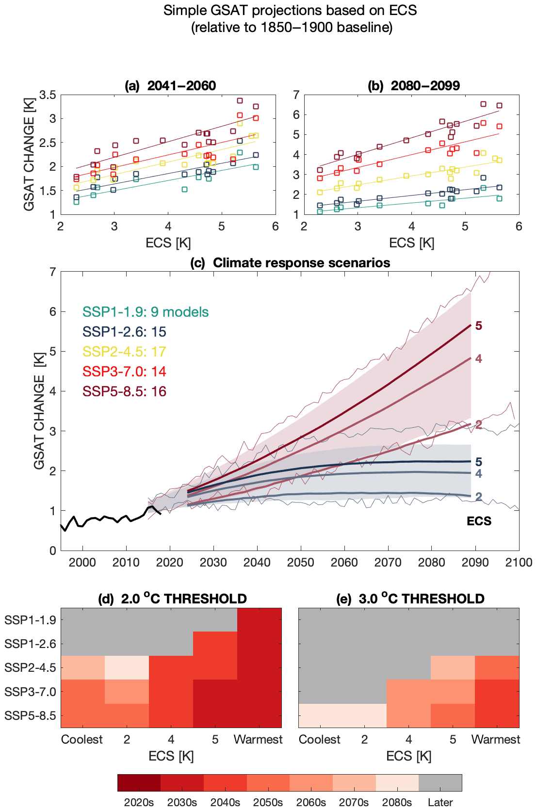
Figure 1Scenarios for global mean surface air temperature (GSAT) derived from CMIP6 projections. Panels (a, b) show regressions, for each SSP, of simulated mean GSAT for a range of models onto each model's own estimated ECS value, for two example 20-year periods. Where multiple ensemble members are available, we have used the ensemble mean response. The simulations are first referenced to the mean of 1995–2014 and baselined to an approximate pre-industrial level using an observed change from 1850–1900 to 1995–2014 of 0.76 C using HadCRUT4 (Morice et al., 2012). Panel (c) shows three climate response scenarios (thick lines) assuming ECS values of 2, 4 and 5 C, for two SSPs (SSP5-8.5, red, and SSP1-2.6, blue), along with the 5 %–95 % simulated range (shaded) and the simulations with the largest and smallest responses at the end of the century (thin lines). Panels (d, e) show the decade in which 2 and 3 C GSAT thresholds are first crossed as a function of climate response scenario and emissions scenario. Grey shading indicates that the threshold is not crossed by 2090 (i.e. the 20-year average of 2081–2100). Note that (1) the SSPs considered are not equally spaced in terms of estimated radiative forcing; (2) GSAT declines in the latter part of the century for some SSPs and, in some cases, may fall back below one of the thresholds shown, but we do not include that possibility in panels (d, e); and (3) a different reference period choice would produce different ranges (Hawkins and Sutton, 2016), especially for the near term; we do not consider this sensitivity here and do not analyse a threshold crossing of 1.5 C for this reason.

Download

Figure 1 also illustrates projections for the most and least rapidly warming models under each SSP. In the absence of counter evidence, these projections might also be considered physically plausible, so these projections offer alternative – more extreme – choices for high-impact scenarios. Such scenarios are likely to be less robust because of their reliance on single model results.

To inform risk assessments, scenarios must be combined with quantification of impacts. There is no single metric of impact: many variables are relevant to policy and decision making. As a simple illustration, we consider here the time of crossing specific temperature thresholds. This variable is important for climate policy following the framing of the Paris Agreement in terms of ambitions to stay below specific levels of GSAT relative to pre-industrial climate. Figure 1d and e illustrate the year in which the 2 and 3 C warming thresholds are crossed, as a function of socioeconomic scenario and climate response scenario. It is immediately apparent that whether and when the thresholds are crossed depend as much on the response scenario as on the forcing scenario. For example, under SSP1-2.6, the 2.0 C threshold is only crossed under the highest ECS scenarios; under SSP3-7.0 and SSP5-8.5, the 5 C ECS scenario yields crossing times 2–3 decades earlier than the 2 C ECS scenario. A notable feature of Fig. 1c is that, before 2060, the 5 C ECS scenario for SSP1-2.6 (low emissions) is warmer than the 2 C ECS scenario for SSP5-8.5 (high emissions). These results illustrate very clearly that climate response scenarios are just as relevant to mitigation policy as are socioeconomic scenarios. The development of robust policies must consider both factors, including explicit attention to high-impact scenarios, such as the 2 and 5 C ECS scenarios considered here. To fully explore the consequences of climate response scenarios obviously requires the expertise of all three IPCC Working Groups. Therefore, it would be extremely valuable if a common set of climate response scenarios could be investigated and assessed by all three groups. Such an approach would aid development of coherent IPCC Synthesis Reports.

Data availability

The CMIP6 data are obtainable from the British Atmospheric Data Centre (BADC; https://esgf-index1.ceda.ac.uk/projects/cmip6-ceda/ last access: 18 August 2020; WCRP, 2020). Values for ECS can be calculated with the Earth System Model Evaluation Tool (ESMValTool). The code for calculating ECS is included in the ESMValTool version 2.0 release (Eyring et al., 2020, https://doi.org/10.5194/gmd-13-3383-2020; Andela et al., 2020, https://doi.org/10.5281/zenodo.3759523).

Author contributions

The idea emerged from discussions between the authors. RTS took the lead in writing the text. EH led the analysis and also contributed to writing the text.

Competing interests

Ed Hawkins is a lead author of Chapter 1 of the Working Group 1 contribution to IPCC AR6.

Acknowledgements

We thank Christine McKenna and the CONSTRAIN project for providing CMIP6 GSAT data, and Karl Alterskjar and Piers Forster for providing the CMIP6 ECS values.

Financial support

This research has been supported by the Natural Environment Research Council and the National Centre for Atmospheric Science.

Review statement

This paper was edited by Gabriele Messori and reviewed by four anonymous referees.

References

Andela, B., Brötz, B., de Mora, L., Drost, N., Eyring, V., Koldunov,N., Lauer, A., Mueller, B., Predoi, V., Righi, M., Schlund, M., Vegas-Regidor, J., Zimmermann, K., Adeniyi, K., Amarjiit, P.,Arnone, E., Bellprat, O., Berg, P., Bock, L., Caron, L.-P., Carvalhais, N., Cionni, I., Cortesi, N., Corti, S., Crezee, B., Davin, E. L., Davini, P., Deser, C., Diblen, F., Docquier, D., Dreyer, L., Ehbrecht, C., Earnshaw, P., Gier, B., Gonzalez-Reviriego, N., Goodman, P., Hagemann, S., von Hardenberg, J., Hassler, B., Hunter, A., Kadow, C., Kindermann, S., Koirala, S., Lledó, L., Lejeune, Q., Lembo, V., Little, B., Loosveldt-Tomas, S., Lorenz, R., Lovato, T., Lucarini, V., Massonnet, F., Mohr, C. W., Pérez-Zanón, N., Phillips, A., Russell, J., Sandstad, M., Sellar, A., Senftleben, D., Serva, F., Sillmann, J., Stacke, T., Swaminathan, R., Torralba, V., and Weigel, K.: ESMValTool (Version v2.0.0b4), Zenodo, https://doi.org/10.5281/zenodo.3759523, 2020. 

Eyring, V., Bock, L., Lauer, A., Righi, M., Schlund, M., Andela, B., Arnone, E., Bellprat, O., Brötz, B., Caron, L.-P., Carvalhais, N., Cionni, I., Cortesi, N., Crezee, B., Davin, E. L., Davini, P., Debeire, K., de Mora, L., Deser, C., Docquier, D., Earnshaw, P., Ehbrecht, C., Gier, B. K., Gonzalez-Reviriego, N., Goodman, P., Hagemann, S., Hardiman, S., Hassler, B., Hunter, A., Kadow, C., Kindermann, S., Koirala, S., Koldunov, N., Lejeune, Q., Lembo, V., Lovato, T., Lucarini, V., Massonnet, F., Müller, B., Pandde, A., Pérez-Zanón, N., Phillips, A., Predoi, V., Russell, J., Sellar, A., Serva, F., Stacke, T., Swaminathan, R., Torralba, V., Vegas-Regidor, J., von Hardenberg, J., Weigel, K., and Zimmermann, K.: Earth System Model Evaluation Tool (ESMValTool) v2.0 – an extended set of large-scale diagnostics for quasi-operational and comprehensive evaluation of Earth system models in CMIP, Geosci. Model Dev., 13, 3383–3438, https://doi.org/10.5194/gmd-13-3383-2020, 2020. 

Field, C. B., Barros, V. R., Mastrandrea, M. D., Mach, K. J., Abdrabo, M. A.-K., Adger, N., Anokhin, Y. A., Anisimov, O. A., Arent, D. J., Barnett, J., Burkett, V. R., Cai, R., Chatterjee, M., Cohen, S. J., Cramer, W., Dasgupta, P., Davidson, D. J., Denton, F., Döll, P., Dow, K., Hijioka, Y., Hoegh-Guldberg, O., Jones, R. G., Joner, R. N., Kitching, R. L., Kovats, R. S., Larsen, J. N., Lin, E., Lobell, D. B., Losada, I. J., Magrin, G. O., Marengo, J. A., Markandya, A., McCarl, B. A., McLean, R. F., Mearns, L. O., Midgley, G. F., Mimura, N., Morton, J. F., Niang, I., Noble, I. R., Nurse, L. A., O'Brien, K., Oki, T., Olsson, L., Oppenheimer, M., Overpeck, J. T., Pereira, J. J., Poloczanska, E. S., Porter, J. R., Pörtner, H.-O., Prather, M. J., Pulwarty, R. S., Reisinger, A., Revi, A., Romero-Lankao, P., Ruppel, O. C., Satterthwaite, D. E., Schmidt, D. N., Settele, J., Smith, K. R., Stone, D. A., Suarez, A. G., Tschakert, P., Valentini, R., Villamizar, A., Warren, R., Wilbanks, T. J., Wong, P. P., Woodward, A., and Yohe, G. W.: IPCC: Summary for policymakers, Climate Change 2014: Impacts, Adaptation, and Vulnerability, Cambridge University Press, Cambridge, 1–32, 2014.  

Forster, P. M., Maycock, A. M., McKenna, C. M., and Smith, C. J.: Latest climate models confirm need urgent mitigation, Nat. Clim. Change, 10, 7–10, https://doi.org/10.1038/s41558-019-0660-0, 2020. 

Hawkins, E. and Sutton, R.: The potential to narrow uncertainty in regional climate predictions, B. Am. Meteorol. Soc., 90, 1095–1107, 2009. 

Hawkins, E. and Sutton, R.: Connecting climate model projections of global temperature change with the real world, B. Am. Meteorol. Soc., 97, 963–980, https://doi.org/10.1175/BAMS-D-14-00154.1, 2016. 

King, D., Schrag, D., Dadi, Z., Qui, Y., and Ghosh, A: Climate change: a risk assessement, Cambridge University Centre for Science and Policy, Cambridge, UK, 2015. 

Morice, C. P., Kennedy, J. J., Rayner, N. A., and Jones, P. D.: Quantifying uncertainties in global and regional temperature change using an ensemble of observational estimates: The HadCRUT4 data set, J. Geophys. Res.-Atmos., 117, D08101, https://doi.org/10.1029/2011JD017187, 2012.  

Shepherd, T. G., Boyd, E., Calel, R. A., Chapman, S. C., Dessai, S., Dima-West, I. M., Fowler, H. J., James, R., Maraun, D., Martius, O., Senior, C. A., Sobel, A. H., Stainforth, D. A., Tett, S. F. B., Trenberth, K. E., van den Hurk, B. J. J. M., Watkins, N. W., Wilby, R. L., and Zenghelis, D. A.: Storylines: An alternative approach to representing uncertainty in physical aspects of climate change, Climatic Change, 151, 555–571, https://doi.org/10.1007/s10584-018-2317-9, 2018. 

Sutton, R. T.: ESD Ideas: a simple proposal to improve the contribution of IPCC WGI to the assessment and communication of climate change risks, Earth Syst. Dynam., 9, 1155–1158, https://doi.org/10.5194/esd-9-1155-2018, 2018. 

Sutton, R.: Climate science needs to take risk assessment much more seriously, B. Am. Meteorol. Soc., 100, 1637–1642, https://doi.org/10.1175/BAMS-D-18-0280.1, 2019. 

WCRP: WCRP Coupled Model Intercomparison Project (Phase 6), available at: https://esgf-index1.ceda.ac.uk/projects/cmip6-ceda/, last access: 18 August 2020. 

1

The presentation of “raw” (i.e. uncorrected) CMIP projections has been supported in several previous WGI reports by an assessment that the 5 %–95 % CMIP range is the likely range (66 % probability) of the future climate response, at least for the long term. However, emerging results from CMIP6 suggest that a similar assessment is unlikely to be tenable for AR6. (In particular, several models show significantly higher equilibrium climate sensitivity (ECS) than the previous generation of CMIP5 models, and their ECS values fall outside the AR5-assessed likely range; Forster et al., 2020.)

2

These scenarios are very similar in concept to the “storylines” advocated by Shepherd et al. (2018).

3

A further attraction of basing global response scenarios on ECS is that the same scenarios could be used in multiple assessment cycles, providing policy makers with helpful continuity between reports.

Download
Short summary
Policy making on climate change routinely employs socioeconomic scenarios to sample the uncertainty in future forcing of the climate system, but the Intergovernmental Panel on Climate Change has not employed similar discrete scenarios to sample the uncertainty in the global climate response. Here, we argue that to enable risk assessments and development of robust policies this gap should be addressed, and we propose a simple methodology.
Special issue
Altmetrics
Final-revised paper
Preprint