Dating hiatuses: a statistical model of the recent slowdown in global warming and the next one

Much has been written about the so-called hiatus or pause in global warming, also known as the stasis period, the start of which is typically dated to 1998. HadCRUT4 global mean temperatures slightly decreased over the 1998–2013 period, although a simple statistical model predicts that they should have grown by 0.016 ^∘C/yr, in proportion to the increases in the concentrations of well-mixed greenhouse gases (WMGHGs) and ozone. We employ a statistical approach to assess the contributions of model forcings and natural variability to the hiatus. Our point estimates suggest that none of the model forcings explain more than one-third of the missing heat, accounting for the upper bound of the confidence interval on the effect of tropospheric aerosols, which is the most prominent yet most uncertainly measured of the model forcings that could explain the missing heat. The El Niño–Southern Oscillation (ENSO) explains up to about one-third of the missing heat, and two-thirds and possibly up to 81 % is explained by the unusually high temperature of 1998. Looking forward, the simple model also fails to explain the large increases since then (0.087 ^∘C/yr from 2013 to 2016). This period coincides with another El Niño, but the ENSO fails to satisfactorily account for the increase. Instead, we propose a semiparametric cointegrating statistical model that augments an energy balance model with a novel multi-basin measure of the oceans' multidecadal temperature cycles. The model partially explains the recent slowdown and explains all of the subsequent warming. The natural cycle suggests the possibility – depending in part on the rate of increase of WMGHG concentrations – of a much longer hiatus over the period from roughly 2023 to 2061, with potentially important implications for policy evaluation.

1 Introduction

There is a well-established physical and statistical link between temperatures and anthropogenic and natural climate forcings. A simple linear cointegrating regression of the HadCRUT4 global mean temperature anomaly (GMT) onto the radiative forcings given by Hansen et al. (2017) explains 88 % of the variation in mean temperature using variations in these forcings. Constraining all but volcanic forcings to have a common coefficient in the regression explains 84 %.

Over the period from 1998 to 2013, the second regression, estimated using a canonical cointegrating regression, predicts an increase of 0.239 ^∘C or 0.016 ^∘C/yr on average, in proportion to the increase in well-mixed greenhouse gases (WMGHGs) and ozone over this period. Instead, observed GMT slightly decreased by 0.024 ^∘C or 0.002 ^∘C/yr on average, earning this period the following nicknames: “stasis period”, “hiatus”, or “pause” in global warming. The difference, measured in this way as 0.263 ^∘C or 0.018 ^∘C/yr, is the so-called “missing heat” of the hiatus, which is quite substantial in the context of the aggregate temperature increase since the preindustrial era of 0.85 ^∘C (IPCC, 2013). In contrast, over the 2013–2016 period, temperatures increased by 0.087 ^∘C/yr, much faster than this simple statistical model predicts.

Our notion of hiatus is roughly consistent with that of Meehl et al. (2011), Kosaka and Xie (2013), and Drijfhout et al. (2014), who reference the apparent hiatus in global warming with respect to the heat flux from greenhouse gases or model forcings more generally. Instead, some authors refer to the hiatus with respect to temperature changes or a trend over an earlier period (Schmidt et al., 2014; Karl et al., 2015; Yao et al., 2016; and Medhaug et al., 2017), while some authors refer to the hiatus without any explicit baseline. Linking missing heat to contemporaneous model forcings is physically appealing, and our empirical evidence suggests that our measure of missing heat comes from a cointegrating regression,¹ so the approach is also statistically appealing. A slowdown or hiatus in global warming as we have defined it does not require a similar slowdown in forcings. On the contrary, such a hiatus is defined in spite of continuing increases in WMGHG concentrations.

What caused this hiatus? Various studies attribute it to one or more of the following: (a) natural variability of the ocean cycles, particularly the Atlantic Multidecadal Oscillation (AMO), the Pacific Decadal Oscillation, and the El Niño–Southern Oscillation (ENSO) (Kosaka and Xie, 2013; Steinman et al., 2015; Yao et al., 2016); (b) cooling from stratospheric aerosols released by volcanic activity (Vernier et al., 2011; Neely et al., 2013); (c) variability in the solar cycle (Huber and Knutti, 2014); (d) a change in the oceans' heat uptake and a weakening of the thermohaline circulation, particularly the Atlantic Meridional Overturning Circulation (AMOC) (Meehl et al., 2011; Drijfhout et al., 2014; Chen and Tung, 2014, 2016); (e) increased anthropogenic emissions of sulfur dioxide from bringing a large number of coal-burning power plants online in China (Kaufmann et al., 2011); and (f) coverage bias or poor data in general (Cowtan and Way, 2014; Karl et al., 2015). Schmidt et al. (2014), Pretis et al. (2015), and Medhaug et al. (2017) emphasize the need to account for multiple explanations for the hiatus.

Keenlyside et al. (2008) note an acceptance in the literature that the AMO and, more generally, multidecadal periodic global temperature fluctuations are related to the AMOC. Drijfhout et al. (2014) posit a physical link through changes in heat uptake across multiple oceans. Specifically, a weakening (strengthening) of the AMOC, meaning less (more) convection and turbulent heat loss, leads to increased (decreased) net heat uptake and, therefore, lower (higher) surface temperatures. The change in net heat uptake occurs across multiple ocean basins, so we label the resulting multidecadal temperature cycle the “Oceanic Multidecadal Oscillation” (OMO). In other words, the OMO is the global sea surface temperature fluctuation resulting from changes in the thermohaline circulation. The OMO contrasts with the AMO in scope – the latter is defined for the North Atlantic – but the two may be highly correlated with similar periodicities.

We propose a new method to measure the OMO, recognizing the possibility of heterogeneous long-term effects of anthropogenic forcings on ocean basins and allowing for a multi-basin contribution to global mean temperatures, in the spirit of Drijfhout et al. (2014) and Wyatt and Curry (2014). The method allows an improvement over the linear detrending method of Enfield et al. (2001) or a single-ocean approach such as the AMO signal estimated by Trenberth and Shea (2006). Not only do we estimate the mean OMO, but we also estimate a global distribution representing the contribution of the OMO to spatially disaggregated sea surface anomalies. In doing so, we carefully decompose the distribution of temperature anomalies into components with long-memory, low-frequency, stochastic trending behavior (mapped to forcings from WMGHGs); with short-memory, medium-frequency, cyclical behavior (the OMO); and with short-memory, high-frequency, idiosyncratic behavior.

We utilize a semiparametric cointegration statistical approach (Park et al., 2010), with widely used and publicly available data sets to estimate an energy balance model (EBM) similar to the well-known model of North (1975) and North and Cahalan (1981). The estimated OMO enters the model non-parametrically, as does the quasi-periodic Southern Oscillation index (SOI), a common proxy for the ENSO. However, information criteria select a linear specification for the latter.

We find that the solar cycle and multidecadal ocean cycle have warmed rather than cooled over the period from 1998 to 2013, so they cannot account for the missing heat. Volcanoes, tropospheric aerosols and surface albedo, and ENSO account for about 1 %, 19 %, and 24 % of the missing heat of the hiatus, respectively. The upper bounds on the uncertainty intervals for the latter two are both about one-third. An even simpler explanation – that the hiatus is defined by starting in an unusually warm year, even taking El Niño into account – explains about two-thirds of the missing heat, a result that echoes previous authors (e.g., Medhaug et al., 2017). A model that takes all but the abovementioned residual into account explains about 42 %.

Roberts et al. (2015) speculate that the hiatus could last through the end of the decade, and Chen and Tung (2014) and Knutson et al. (2016) make stronger statements about its continuation. If so, then the unusually warm years of 2015 and 2016 are outliers, and global temperatures can be expected to stabilize or cool in the next decade. On the contrary, our proposed model explains nearly all of the more recent record warm years, overshooting the record high anomaly of 0.773 ^∘C in 2016 by less than 0.001 ^∘C. This result provides conclusive statistical evidence that the hiatus is over. In other words, we date the end of the recent hiatus prior to 2015.

Can we expect a future hiatus or slowdown? If so, when? We find that the two most influential nonseasonal drivers of global aggregate temperature change are the long-term contribution of WMGHGs and the fairly predictable OMO with a period of 76 years, consistent with the 65- to 80-year period estimated for the AMO in the literature (Knight et al., 2005; Trenberth and Shea, 2006; Keenlyside et al., 2008; Gulev et al., 2013; Wyatt and Curry, 2014). Although the OMO cannot explain the recent hiatus, it can explain past multidecadal cooling or hiatus periods, such as the decades following the temperature spikes in about 1877 and 1943.

For the period from 1944 to 1976, Kaufmann et al. (2006a) note that the decrease in the net radiative forcing resulting from an increase in anthropogenic sulfur emissions approximately offset the increase in the net forcing from an increase in WMGHGs. Aside from the uncertainty in measuring forcing from sulfur emissions, this offset nicely shows the relationship between the OMO and temperatures: while the OMO declined by an average of 0.016 ^∘C/yr, temperature also declined by an average of 0.012 ^∘C/yr. The decline in temperature over this period may be explained both by a decline in the OMO and an increase in sulfur emissions.

If we condition the model on future forcings with growth rates similar to RCP8.5, we can expect temperatures to increase with a possible slowdown but without any future hiatus. However, if we condition on future forcings with the same average annual rate as that of the past 76 years, similarly to RCP6.0, we expect a multidecadal hiatus from approximately 2023 to 2061. Note that our finding of a warm period separating the previous slowdown from the next one is exactly consistent with the recent projection of warming from 2018 to 2022 by Sévellec and Drijfhout (2018) using a different model and method.

2 Empirical results

We utilize forcings data² over the period from 1850 to 2016 from Hansen et al. (2017). We create two radiative forcing series: the sum of forcings from WMGHGs (primarily CO₂, CH₄, N₂O, and CFCs), ozone, tropospheric aerosols and surface albedo, and solar irradiance, denoted by h₁, and that from volcanoes, denoted by h₂. Shindell (2014) suggests the possibility that forcings due to aerosols and ozone may have effects that are different from those of WMGHGs. By aggregating all nonvolcanic forcings into h₁, we are instead following studies such as Estrada et al. (2013) and Pretis (2015). A Wald test shows no statistically significant difference (p value of 0.61) between models with and without the restriction imposed³.

Some authors, such as Estrada et al. (2013), ignore volcanoes in statistical estimation of EBMs. Leaving out volcanoes is statistically justified by the apparent lack of correlation of this series with the other forcings. Relegating that series to the error term may affect statistical uncertainty, but it should not bias the estimates of the effect of h₁. Because one of our goals is to assess the impact of volcanic activity on the slowdown, we include volcanoes. However, we allow for a separate coefficient on h₂ in order to accommodate the suggestion of Lindzen and Giannitsis (1998) of a smaller sensitivity parameter for physical models that include volcanic forcing.

We use HadCRUT4 and HadSST3 temperature anomaly data, measured relative to 1961–1990, from Morice et al. (2012) and Kennedy et al. (2011a,b), respectively.⁴ In order to estimate the global distribution of the OMO, monthly HadSST3 data observed over a 5^∘ latitude by 5^∘ longitude grid resolution are pooled into years over the 1850–2016 period (167 years of data). The HadCRUT4 data set combines HadSST3 for sea and CRUTEM4 for land, so the temperatures from HadCRUT4 and HadSST3 are comparable. However, using only HadSST3 for the distribution ensures that grid boxes containing both land and ocean stations will contain only ocean measurements in the distribution.

The Supplement contains a detailed description of the methodology used to estimate the distribution of the OMO, the probability density function of which we denote by f_t(r) for year t with support $[r^{-},r^{+}]$ (see the bottom panel of Fig. S3). Our methodology omits both long-term temporal temperature trends to avoid cointegration with h_t and idiosyncratic noise to avoid overfitting very short-term fluctuations in GMT using sea surface temperatures. It is intuitively similar to band-pass filters used to identify cycles in economic and other oscillating time series, but it is not executed in the frequency domain.

Consistent with an EBM, filtering long-term stochastic trends (low frequency on the spectrum) is accomplished by regressing out the anthropogenic signal (see Fig. S1 of the Supplement). In contrast, linear detrending (Enfield et al., 2001) unnecessarily assumes a constant growth rate of the anthropogenic signal. More modern approaches, such as that of Trenberth and Shea (2006) and Lenton et al. (2017), also filter the anthropogenic signal, but they do so indirectly as a difference between temperature series both subjected to the same stochastic trend.

Detrending results in a noisy oscillation. High-frequency filtering could be accomplished using spectral methods if the time series were long enough or if the noise were “quiet” enough. However, it is difficult to identify a cycle with a 65- to 80-year period from a time series of 167 years in the presence of high-frequency cycles with substantial amplitudes, such as the ENSO and solar cycle. By focusing on a single periodic function, we narrow the desired frequency band enough to identify the cycle and to estimate it very transparently in the time domain. Specifically, we fit the stochastically detrended temperatures to a single periodic function (see Table S1 and Fig. S4).

We base our statistical model on an EBM given by

$$\begin{array}{}\text{(1)}& T^a={\mathit{h}}^{*}{}^{\prime }\mathit{\alpha }+\underset{r^{-}}{\overset{r^{+}}{\int }}b\left(r\right)f\left(r\right)dr+c\left(S\right)+\mathit{\eta },\end{array}$$

where T^a is the global mean temperature anomaly (GMT), ${\mathit{h}}^{*}=(\mathrm{1},h_{\mathrm{1}},h_{\mathrm{2}}{)}^{\prime }$ is global forcing, S is the Southern Oscillation index (SOI; Ropelewski and Jones, 1987) used to proxy ENSO quasi-periodic cycles,⁵ $\mathit{\alpha }=({\mathit{\alpha }}_{\mathrm{0}},{\mathit{\alpha }}_{\mathrm{1}},{\mathit{\alpha }}_{\mathrm{2}}{)}^{\prime }$ is a coefficient vector, and η is an error term.

A detailed derivation of the EBM from a more familiar EBM similar to those of North (1975), North and Cahalan (1981), and North et al. (1981), among others, is provided in the Supplement. A primary intuition for the derivation is that the nonlinear functions b(r) and c(S) allow the oceans' heat uptake to vary over multidecadal and interannual oscillations.

In order to estimate the EBM in Eq. (1) non-parametrically in b(r) and c(S), we attach time subscripts and write

$$\begin{array}{}\text{(2)}& T_t^a={\mathit{h}}_t^{*}{}^{\prime }\mathit{\alpha }+{\mathit{x}}_t^{\prime }\mathit{\gamma }+{\mathit{w}}_t^{\prime }\mathit{\delta }+{\mathit{\eta }}_t,\end{array}$$

where ${\mathit{x}}_t=(x_{\mathrm{1}t},\mathrm{\dots },x_{m_{T}t}{)}^{\prime }={\int }_{r^{-}}^{r^{+}}{\mathit{b}}_{\mathrm{1}:m_T}(r\left)f_t\right(r)\mathrm{d}r$ with ${\mathit{b}}_{\mathrm{1}:m_T}\left(r\right)=\left(b_{\mathrm{1}}\right(r),\mathrm{\dots },b_{m_T}(r){)}^{\prime }$ and ${\mathit{w}}_t=(w_{\mathrm{1}t},\mathrm{\dots },w_{m_{S}t}{)}^{\prime }={\mathit{c}}_{\mathrm{1}:m_S}(S_t)$ with ${\mathit{c}}_{\mathrm{1}:m_S}\left(S_t\right)=\left(c_{\mathrm{1}}\right(S_t),\mathrm{\dots },c_{m_S}(S_t){)}^{\prime }$ are finite-order series approximations to ${\int }_{r^{-}}^{r^{+}}b\left(r\right)f_t\left(r\right)\mathrm{d}r$ and c(S_t). The error term η_t contains both (serially correlated) stochastic forcings, along the lines of North et al. (1981), and any approximation errors from the series approximations.

2.1 The 1998–2013 episode

The missing heat of the recent hiatus is defined above by the difference between the actual GMT in 2013 and the temperature predicted from increases in the WMGHG and ozone (hereafter referred to as G+Z) alone using the restricted model with $\mathit{\gamma },\mathit{\delta }=\mathrm{0}$ and starting in 1998. The GMT in 1998 was 0.536 ^∘C. Fixing 1998 as the starting year and based on an increase in climate forcings from G+Z of 0.561 W/m² over the 1998–2013 period, the model predicts a GMT of $\mathrm{0.536}+\mathrm{0.561}\times \mathrm{0.426}\simeq \mathrm{0.775}$ ^∘C in 2013, where 0.426 is the canonical cointegrating regression (CCR) estimate of α₁ in the model in Eq. (2) with $\mathit{\gamma },\mathit{\delta }=\mathrm{0}$ (see Table S2 in the Supplement), with a 90 % confidence interval of (0.756,0.795) ^∘C.⁶ In contrast, the observed GMT is 0.512 ^∘C in 2013, so that the difference, $\mathrm{0.775}-\mathrm{0.512}\simeq \mathrm{0.263}$ ^∘C (0.244,0.283) ^∘C, represents the missing heat. The 1998–2013 episode is illustrated by the missing heat in Fig. 1. Figure 2 shows the contributions of key potential explanations of the hiatus as a percentage of the missing heat with the 90 % confidence intervals.

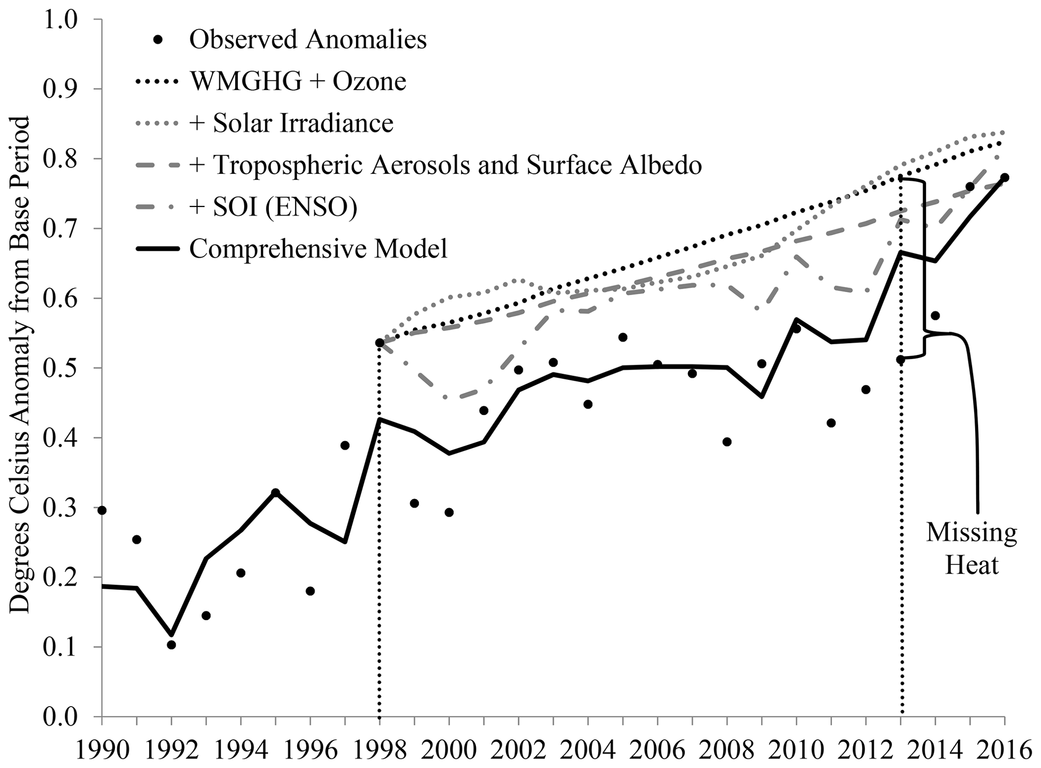
Figure 1 A visual anatomy of the 1998–2013 episode. The hiatus is defined by the missing heat in 2013 relative to that predicted by increases in the WMGHG and ozone forcings since 1998. Plots crossing the missing heat help to explain it (tropospheric aerosols and surface albedo, ENSO, and the comprehensive model are shown), whereas those passing above the missing heat exacerbate it (solar irradiance is shown).

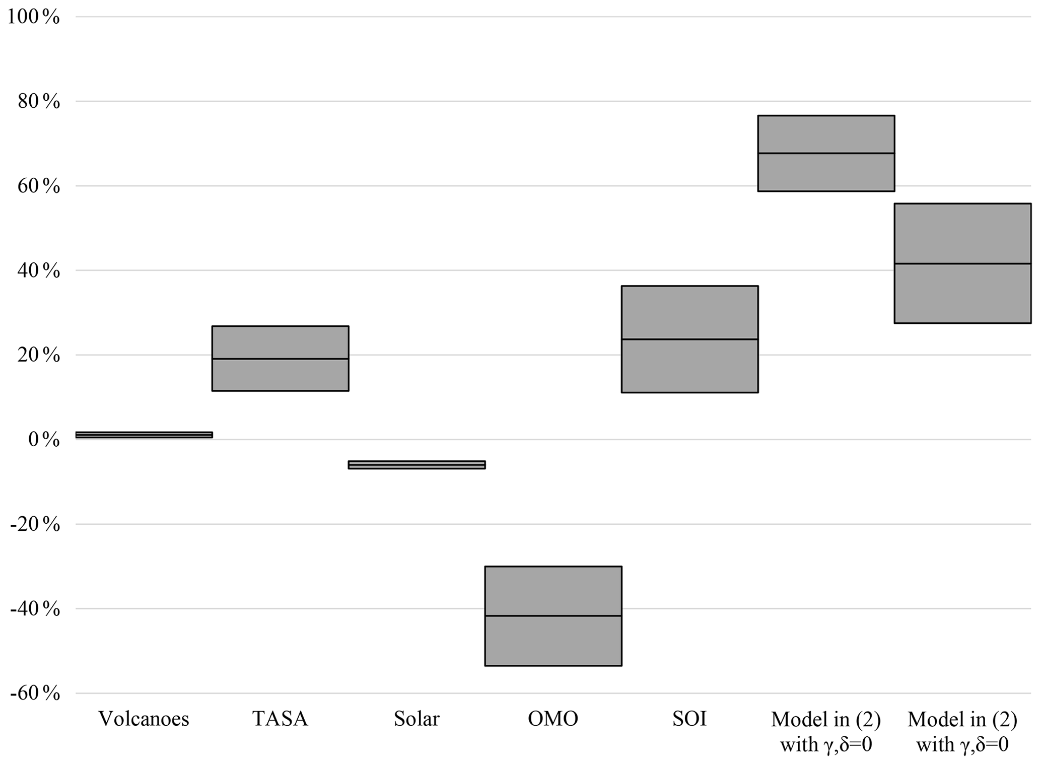
Figure 2 Estimated contributions of key potential explanations of the 1998–2013 episode. Positive percentages of the missing heat (0.263 ^∘C) help to explain it, whereas negative percentages of the missing heat exacerbate the puzzle. Tropospheric aerosols and surface albedo are abbreviated as “TASA”. The 90 % confidence intervals are shown by the two boxes, and the border between the boxes represents the point estimates.

One way to try to explain the missing heat is to “turn on” some of the other forcings in the model. To that end, we estimate the model in Eq. (2) with both $\mathit{\gamma },\mathit{\delta }\ne \mathrm{0}$ (unrestricted) and $\mathit{\gamma },\mathit{\delta }=\mathrm{0}$ (restricted). Least squares is expected to be consistent, but we use the CCR approach of Park et al. (2010) in order to asymptotically, normally estimate the coefficients and consistently estimate the standard errors for cointegrated temperatures and forcings. A number of previous studies, such as Kaufmann et al. (2006a, b, 2010, 2013) and Pretis (2015), have provided physical and statistical evidence in favor of a cointegrating relationship. As explained in the Supplement, this procedure also corrects for uncertainty in the forcings data.

Adding only volcanoes to G+Z decreases forcings by 0.036 W/m². Predicted GMT decreases by only 0.003 ^∘C (0.001,0.004) ^∘C or about 1.1 % (0.5,1.7) % of (the point estimate of) the missing heat. In the data, forcing from stratospheric aerosols is attributed to volcanic activity, whereas forcing from tropospheric aerosols is attributed to anthropogenic sulfur dioxide emissions. Vernier et al. (2011) refute previous studies that attribute an increase in stratospheric aerosols to emissions. While those authors do not discuss the effect of volcanic activity on the hiatus directly, their Fig. 5 suggests that the stratospheric aerosol levels from Mt. Pinatubo subsided until about 1997, and the increase since then has been relatively small.

Similarly, adding only tropospheric aerosols and surface albedo to G+Z decreases forcings by 0.118 W/m². Predicted GMT decreases by 0.050 ^∘C (0.030,0.070) ^∘C, or 19.1 % (11.5,26.8) % of the missing heat. An alternative measure of forcings from tropospheric aerosols based on the sulfur emissions data of Hoesly et al. (2018) predicts GMT increasing by 0.003 ^∘C $\left(-\mathrm{0.014},\mathrm{0.020}\right)$ ^∘C, or exacerbating the missing heat by 1.3 % $\left(-\mathrm{5.7},\mathrm{8.3}\right)$ %. The Supplement contains more details of how the alternative data were employed and additional empirical results based on them.

That anthropogenic aerosol emissions appear to explain some of the missing heat using the Hansen et al. (2017) data is consistent with the findings of Storelvmo et al. (2016) and Kaufmann et al. (2011). Unfortunately, although the interval estimate using these tropospheric aerosol data explicitly account for measurement error, it does not cover the point estimate using the data of Hoesly et al. (2018), and vice versa. In short, the effect is quite uncertain using either data set.

Solar irradiance increases forcings by 0.037 W/m², so that the predicted GMT increases by 0.016 ^∘C (0.013,0.018) ^∘C, exacerbating the missing heat by 6.0 % (5.1,6.9) %. There is a decline from 2002 to 2006, but the net effect of solar from 1998 to 2013 is to increase temperature – not to decrease it. To the extent that solar contributed to the slowdown by decreasing temperatures, the results suggest that solar alone is not sufficient. This finding is not inconsistent with that of Schmidt et al. (2014), who examine solar in conjunction with other forcings as an explanation.

The preceding explanations are model forcings, and none of them satisfactorily account for the slowdown either alone or in concert. As previous authors have pointed out, natural variability may play a role, and we now turn to measures of two such types: the OMO and the ENSO.

In order to examine multidecadal oscillations from the OMO as a possible explanation, we let γ≠0, but we keep δ=0. The regressor vector x_t is correlated with the other forcings, and we want to capture the partial effect of the OMO while retaining the total effect of G+Z. In order to do so, we employ the fitted residuals from regressing x_t onto the other forcings as a regressor in the model, rather than using x_t itself. The two approaches – using x_t or its fitted residuals – yield equivalent model fits, but using the fitted residuals fixes the coefficient vector α.

The oscillation exacerbates the missing heat by 0.110 ^∘C (0.079,0.141) ^∘C or 41.7 % (30.0,53.5) %. By itself, the fitted OMO worsens the puzzle in the sense that the predicted temperature in 2013 increases to $\mathrm{0.775}+\mathrm{0.110}=\mathrm{0.885}$ ^∘C. The reason for the increase is that the OMO appears to be increasing rather than decreasing during this period. This result contrasts sharply with that of Yao et al. (2016), who attribute the hiatus to a much shorter oceanic cycle of 60 years.

The ENSO is quasi-periodic with a period of about 5–6 years. However, roughly every three El Niño episodes are so-called “super El Niños” with much higher amplitudes than the intervening episodes. In other words, the ENSO also oscillates at a decadal scale (roughly 15 to 18 years). The last two peaks of the longer oscillation were in 1997–1998 and 2015–2016, coinciding with the beginning and end of the 1998–2013 episode. Letting δ≠0 but keeping γ=0 yields an increase in the normalized and orthogonalized SOI of 1.162 and, thus, a decrease of 0.062 ^∘C (0.029,0.095) ^∘C, so that the ENSO explains 23.7 % (11.1,36.3) % of the missing heat.

All of the explanations so far ignore to some extent that the starting year matters, as has been pointed out by previous authors (e.g., Medhaug et al., 2017). Not only was 1998 an El Niño year, it was an anomalously warm one. Suppose that the temperature anomaly in 1998 had been equal to that in 1997 (0.389 ^∘C). The same exercise of defining the hiatus using growth rates predicted by G+Z results in a 2013 temperature anomaly of $\mathrm{0.389}+\mathrm{0.561}\times \mathrm{0.426}=\mathrm{0.628}$ ^∘C, a decrease of $\mathrm{0.775}-\mathrm{0.628}=\mathrm{0.147}$ ^∘C, which explains 55.9 % of the missing heat. In other words, half of the puzzle is explained simply by the construction of the puzzle.

The counterfactual of setting the 1998 temperature to that of 1997 seems effective in explaining the slowdown, but it is extremely ad hoc. A similar result is obtained more formally by fitting the model forcings but no natural variation – i.e., by estimating the model in Eq. (2) with $\mathit{\gamma },\mathit{\delta }=\mathrm{0}$. This model predicts the temperature in 1998 to be 0.395 ^∘C – close to that in 1997 – and increasing to 0.597 ^∘C by 2013. In other words, a simple model, including all forcings but without the OMO or the ENSO, explains 0.178 ^∘C (0.155,0.202) ^∘C, or 67.7 % (58.7,76.6) % – more than half – of the missing heat. Looking at the most comprehensive model with $\mathit{\delta },\mathit{\gamma }\ne \mathrm{0}$ gives a qualitatively similar result, explaining 41.6 % (27.5,55.8) %.

This finding suggests that the unusually warm year of 1998 – a residual in the model – accounts for most of the apparent slowdown between 1998 and 2013. It is consistent with the finding of Kosaka and Xie (2013), in the sense that the El Niño year is necessarily followed by La Niña cooling. However, with the results of Pretis et al. (2015) and those using the SOI above in mind, we certainly cannot attribute the slowdown to the ENSO uniquely.

Yet there is a new problem given by the high GMTs of 0.760 ^∘C in 2015 and 0.773 ^∘C in 2016. The restricted model undershoots these temperatures by more than 0.1 ^∘C. Are these simply outliers, as 1998 was? A natural explanation is the ENSO, because 2015 and 2016 were El Niño years. The model with δ≠0 and γ=0 – i.e., with SOI but no OMO – undershoots 2015 by more than 0.1 ^∘C and 2016 by just less than 0.1 ^∘C. In other words, accounting for ENSO does about as poorly as not accounting for ENSO in predicting the temperature in 2015, but it improves the prediction for 2016.

Finally, consider the proposed comprehensive model with $\mathit{\delta },\mathit{\gamma }\ne \mathrm{0}$. The model undershoots 2015 by only 0.042 ^∘C while overshooting 2016 by less than 0.001 ^∘C (see Fig. 1). We interpret these numbers to mean that the recent high temperatures of 2015 and 2016 are attributable more to the smooth, multidecadal, and somewhat predictable OMO than to the higher-frequency quasi-periodic ENSO. As a result, we can say that 2015 and 2016 were not outliers and that increases in global mean temperatures may be expected to continue as the OMO continues to put upward pressure on temperatures. Put more simply, the hiatus that appeared to begin in 1998 ended in 2013.

2.2 The 2023–2061 episode

Wyatt and Curry (2014) emphasize that, although evidence supports a secularly varying oscillation like the one that we estimate, future external forcings may alter the amplitude and period of the cycle. Linear detrending may overemphasize this possibility by giving a stochastically trending series with secular oscillations the appearance of a secularly trending series with quasi-periodic or stochastic oscillations. If the long-term trend is indeed anthropogenic, the former is more appropriate than the latter.

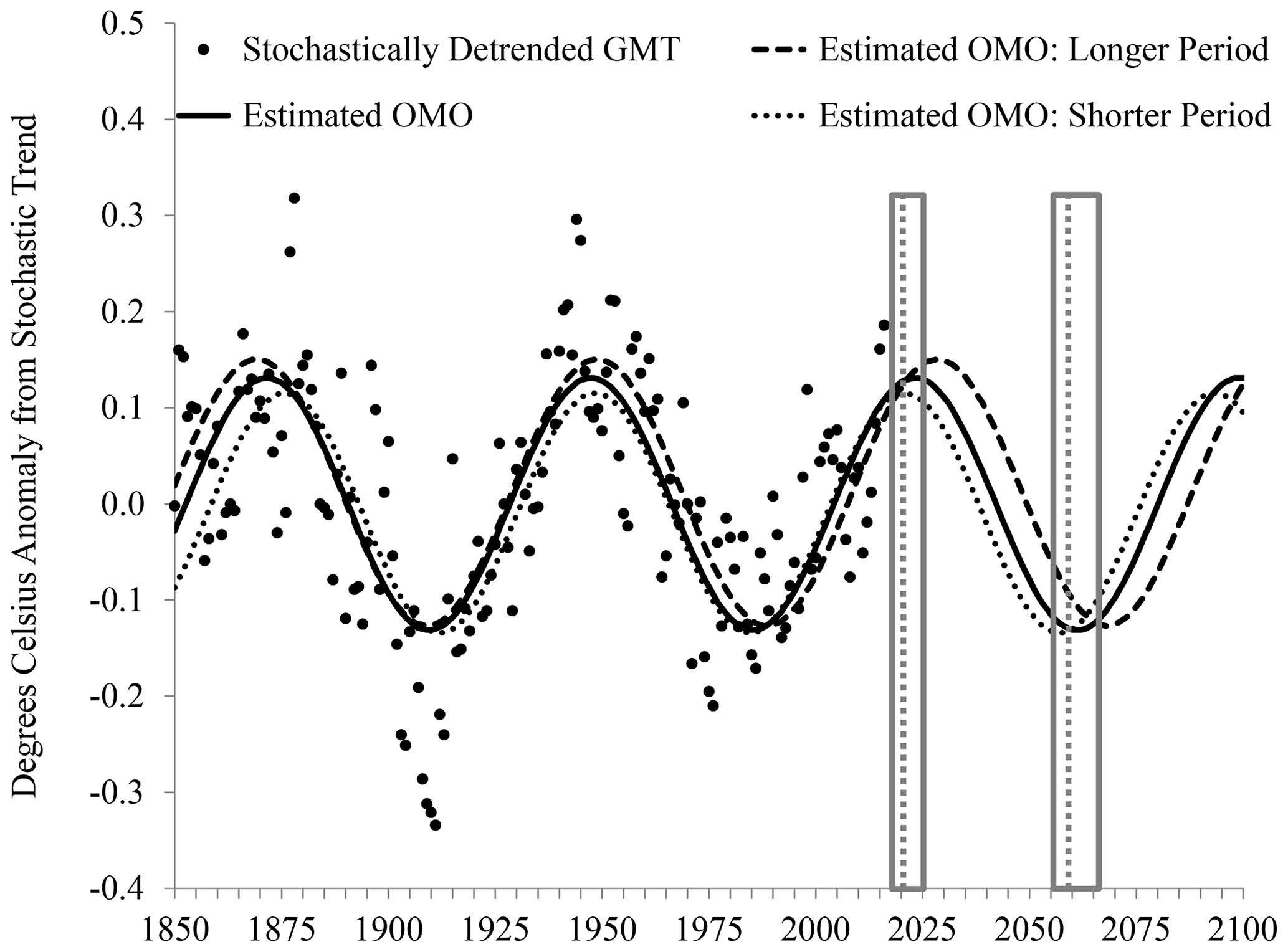
Figure 3 The Oceanic Multidecadal Oscillation (OMO) from 1850 to 2100. The estimated and predicted OMO, with the 90 % confidence interval on the next downturn and subsequent upturn.

We fit a sine function and predict it to 2100, as shown in Fig. 3. After crossing zero before 2005, the sine function continues to increase for roughly $\mathrm{76}/\mathrm{4}=\mathrm{19}$ years until about 2023, and it then decreases for about 38 years until roughly 2061. Figure 3 shows sine functions reflecting a lower and upper 90 % confidence interval for the estimated period. This interval is not a prediction interval for a future year, so the plots do not straddle that of the point forecasts, nor is it constructed from standard errors, which do not reflect correlation of the estimates of the period and phase shift.

Rather, we rely on an AR(1) bootstrap strategy in the spirit of Poppick et al. (2017), which is described in the Supplement. The 90 % bootstrap confidence interval of the estimated period of 76 years is 73 to 80 years. We date the next peak in the sign function as 2023 – likely falling in the interval between 2021 and 2028 – and the next minimum as 2061 – likely falling in the interval between 2057 and 2068. We note that homogeneous linear detrending results in a period of 72 years, while the stochastically detrended AMO of Trenberth and Shea (2006) results in a period of 78 years. Our method, which has the advantages of relating the stochastic trend to forcings by way of a physical model and generates oscillations that are statistically more regular (see the Supplement for details), generates an uncertainty interval that plausibly accounts for uncertainty in the stochastic trend.

A downturn in the temperatures due to the ocean cycle implies a slowdown but not necessarily a hiatus in global warming, because the upward trend in forcings may more than offset the downturn. The model in Eq. (2) may be used to forecast temperature anomalies conditional on changes in one or more forcings. In our forecasts, we condition on volcanic activity remaining at its 2016 level and the SOI remaining at its temporal mean over the 1850–2016 period. We do not forecast the ENSO, because it is not periodic enough that long-term forecasts of the ENSO would be very accurate, and its estimated effect on temperature is not as large as that of the OMO.

We consider two possible scenarios for nonvolcanic forcings, which are closely related to RCP8.5 and RCP6.0. The data in 2016 have already deviated from the RCPs, so we simply match the cumulative growth rates of the CO₂ equivalents of all anthropogenic forcings driving the two RCPs to those of nonvolcanic forcings starting in 2016 in order to generate our two scenarios. RCP8.5 is considered by many to be “business as usual” and the average annual growth implied by RCP8.5 is 0.053 W/m²/yr. Forcings would have to grow at a sustained rate much faster than the recent growth of 0.029 W/m²/yr over the 2013–2016 period – i.e., since the end of the hiatus and beginning of the recent El Niño period. On the other hand, RCP6.0 has an average annual growth of 0.021 W/m²/yr, similar to 0.024 W/m²/yr over the last 76 years – one complete period of the OMO – in order to filter out any multidecadal cyclicity in the forcings themselves.

Two points warrant discussion. First, we are ignoring the recalcitrant component of warming (Held et al., 2010), and we are not using a dynamic model to try to capture short-term dynamics. As a result, our model is set up to make conditional forecasts of roughly 5 to 90 years from the end of the sample. Second, forecasts are conditional on the scenarios mentioned above, but we make no attempt to forecast individual forcings, such as solar or WMGHGs.

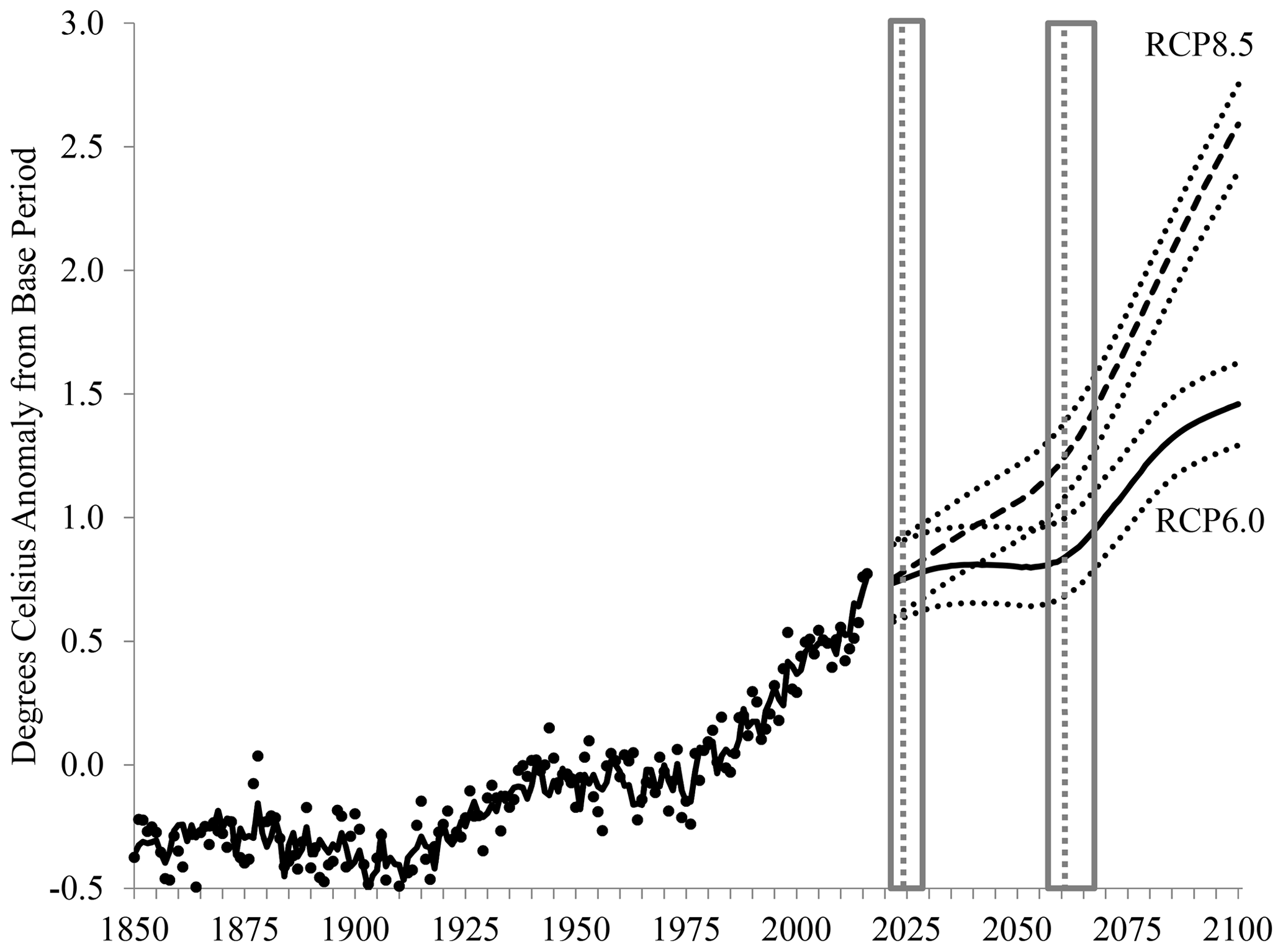
Figure 4 Conditional forecasts of temperature anomalies from 2022 to 2100. Until 2016, dots represent the actual temperature anomaly data, and the solid line represents the temperature anomaly predicted by the model. The scenario labeled RCP8.5 uses RCP8.5 growth rates for anthropogenic forcings from a starting point of 2016; the scenario labeled RCP6.0 similarly uses RCP6.0 growth rates. The 90 % confidence bands are shown.

Figure 4 shows the sample paths of the conditional forecasts under the two scenarios. Under RCP8.5, anthropogenic forcings increase so much that downturns in the OMO cycle are never again powerful enough to force a hiatus in global warming. The global temperature anomaly increases by 0.022 ^∘C/yr (0.019,0.024) ^∘C/yr on average to nearly 3 ^∘C over the base period by 2100. Nevertheless, a slowdown is predicted until about 2061 under RCP8.5, after which point temperature growth is predicted to accelerate to a much faster rate over multiple decades than that of the historical record. Of course, our forecasts are conditional on ENSO being unrealistically flat. A hiatus could again result from a well-timed super El Niño, such as that in 1997–1998.

Under RCP6.0, the temperature increases by about 0.008 ^∘C/yr (0.006,0.010) ^∘C/yr on average. By 2100, temperature anomalies increase to 1.459 ^∘C (1.292,1.626) ^∘C, which is 1.764 ^∘C (1.598,1.931) ^∘C above preindustrial temperatures, because the base period is 0.305 ^∘C above preindustrial temperatures, approximated by the 1850–1879 average. While this interval is still below 2 ^∘C, it exceeds the Paris Agreement goal of 1.5 ^∘C.

We see a substantial ebb and flow of the effect of the OMO cycle on temperatures under RCP6.0. Between 2023 and 2061, the dates identified of the next maximum and minimum of the OMO, the temperature is predicted to grow by only 0.0001 ^∘C/yr – i.e., virtually no growth. In contrast to the average annual growth of anthropogenic forcings of 0.022 W/m²/yr under RCP6.0, this projection clearly suggests a future hiatus period that is much longer than the 1998–2013 episode. However, a very crude rule of thumb forecast suggests the possibility of a super El Niño in approximately 2034, which could break up the hiatus predicted by the OMO.

The variation in temperatures from the OMO is estimated to be 0.262 ^∘C (0.249,0.277) ^∘C. At its predicted nadir in 2061, temperatures are predicted to have increased since 2023 by 0.100 ^∘C (0.098,0.102) ^∘C under RCP6.0 or 0.486 ^∘C (0.479,0.494) ^∘C under RCP8.5, meaning that they would have increased by $\mathrm{0.262}+\mathrm{0.100}=\mathrm{0.362}$ ^∘C under RCP6.0 or $\mathrm{0.262}+\mathrm{0.486}=\mathrm{0.748}$ ^∘C under RCP8.5 without the OMO. Based on the point estimates, we expect the variation in the OMO to mask the underlying warming trend by $\mathrm{1}-\mathrm{0.486}/\mathrm{0.748}=\mathrm{35}$ % under RCP8.5 and by $\mathrm{1}-\mathrm{0.100}/\mathrm{0.362}=\mathrm{72}$ % under RCP6.0.

3 Summary and implications for policy evaluation

It is no exaggeration to say that the 1998–2013 apparent hiatus in the otherwise evident trend of warming global mean temperatures has generated controversy. From a scientific point of view, a number of researchers have put forth differing explanations backed up by plausible physical models joined with sound statistical methods. Because of the critical importance of climate change to human systems – economic, political, etc. – the controversy has spilled over into the arena of public and political debate, where the lack of warming is viewed as empirical validation by those skeptical of global warming. Lack of consensus about the cause only adds to such doubt.

In this paper, we disentangle some of the causes of the 1998–2013 hiatus and subsequent run-up in temperatures using a modern statistical technique, a semiparametric cointegrating regression, based on an energy balance model. Our main findings for this period suggest that the three main factors driving the hiatus were (1) the unusually warm year of 1998, even conditional on the ENSO; (2) the ENSO itself; and (3) the increase in tropospheric aerosols during that period, although the latter is measured with a high degree of uncertainty. Other potential causes that we investigate had considerably less impact or an accelerating rather than confounding impact on rising temperatures. Our statistical model not only explains much of the hiatus but also explains the rapid warming since 2013. We find that this warming marks the end of the hiatus, in contrast to some findings in the literature (e.g., Chen and Tung, 2014; Knutson et al., 2016) but consistent with the results of Sévellec and Drijfhout (2018)

Further, fitting the mean of the distribution of detrended ocean temperature anomalies (an oceanic multidecadal oscillation) to a periodic function enables us to make forecasts of the global mean temperature conditional on forcing scenarios. If forcings grow at the same rate as they have for the past 76 years (the estimated period of the OMO), we can expect a longer hiatus in global warming from about 2023 to about 2061, roughly 3 to 4 decades. The controversy of the recent 15-year hiatus is a precursor to that which may result from a much longer one. Kaufmann et al. (2017) recently showed a correlation between climate skepticism and locally cooler (or less warm) temperatures in the US. If the lack of warming indeed drives doubt, 3 decades of no warming is indeed a long period to fuel skepticism. Nevertheless, on the current trajectory, we can expect the decades following the next hiatus to push well past the 1.5 ^∘C goal of the Paris Agreement and even past 2 ^∘C.

Even though our model makes use of spatially disaggregated sea surface temperatures, our results have nothing to say directly about regional differences in temperature oscillations. As emphasized by Kaufmann et al. (2017) and many other authors, the effects are spatially heterogeneous. Based on the estimated warming trends displayed in Fig. S1 in the Supplement, we speculate that the effect of a future hiatus will be more noticeable in the vicinity of the Pacific and Indian oceans than in the vicinity of the Atlantic Ocean, because the latter has more strongly increasing trends.

It may be useful to assign a probability to the possibility of a future multidecadal hiatus. Such a forecast would require more information and entail more uncertainty than the conditional forecasts above, because a probability distribution would be needed for future forcings. Rather than try to forecast forcings, one could base such a forecast on, say, expert opinion of the likelihood of forcing scenarios. Suppose, for example, that one believes that forcings will increase at an average rate of w per year, where w is a random variable symmetrically distributed around RCP6.0. Figure 4 suggests that, roughly speaking, scenarios with weaker growth will result in a future hiatus, while those with stronger growth will not. Ignoring the uncertainty associated with the conditional forecasts, one with such a belief could make a prediction that a multidecadal hiatus will occur with a probability of roughly 50 %. We emphasize, however, the inherent uncertainty in such an exercise, even taking our allowance for uncertainty in the data and estimates into account.

Our forecasts are conditional on hypothetical concentration pathways. We cannot and do not suggest that policy should be based on our results. Rather, we seek to inform scientists and policymakers of the possibility of a warming hiatus due to a natural cycle. Such a cycle may be expected to have a confounding effect on policy evaluation, because a natural downturn may be mistaken for the effectiveness of mitigation. The quasi-experimental statistical evaluation of such policies must take this effect into account in order to avoid mistaking a failed policy for a successful one.