Disequilibrium of terrestrial ecosystem CO₂ budget caused by disturbance-induced emissions and non-CO₂ carbon export flows: a global model assessment

The global carbon budget of terrestrial ecosystems is chiefly determined by major flows of carbon dioxide (CO₂) such as photosynthesis and respiration, but various minor flows exert considerable influence in determining carbon stocks and their turnover. This study assessed the effects of eight minor carbon flows on the terrestrial carbon budget using a process-based model, the Vegetation Integrative SImulator for Trace gases (VISIT), which included non-CO₂ carbon flows, such as methane and biogenic volatile organic compound (BVOC) emissions and subsurface carbon exports and disturbances such as biomass burning, land-use changes, and harvest activities. The range of model-associated uncertainty was evaluated through parameter-ensemble simulations and the results were compared with corresponding observational and modeling studies. In the historical period of 1901–2016, the VISIT simulation indicated that the minor flows substantially influenced terrestrial carbon stocks, flows, and budgets. The simulations estimated mean net ecosystem production in 2000–2009 as 3.21±1.1 Pg C yr⁻¹ without minor flows and 6.85±0.9 Pg C yr⁻¹ with minor flows. Including minor carbon flows yielded an estimated net biome production of 1.62±1.0 Pg C yr⁻¹ in the same period. Biomass burning, wood harvest, export of organic carbon by water erosion, and BVOC emissions had impacts on the global terrestrial carbon budget amounting to around 1 Pg C yr⁻¹ with specific interannual variabilities. After including the minor flows, ecosystem carbon storage was suppressed by about 440 Pg C, and its mean residence time was shortened by about 2.4 years. The minor flows occur heterogeneously over the land, such that BVOC emission, subsurface export, and wood harvest occur mainly in the tropics, and biomass burning occurs extensively in boreal forests. They also differ in their decadal trends, due to differences in their driving factors. Aggregating the simulation results by land-cover type, cropland fraction, and annual precipitation yielded more insight into the contributions of these minor flows to the terrestrial carbon budget. Considering their substantial and unique roles, these minor flows should be taken into account in the global carbon budget in an integrated manner.

1 Introduction

The terrestrial ecosystem is a substantial sink of atmospheric carbon dioxide (CO₂) at decadal or longer scales and is mainly responsible for interannual variability of the global carbon budget (Schimel et al., 2001; Le Quéré et al., 2018). The current and future carbon budgets of terrestrial ecosystems have a feedback effect on the ongoing climate change, and they thus affect the effectiveness of climate mitigation policies such as the Paris Agreement (Friedlingstein et al., 2014; Seneviratne et al., 2016; Schleussner et al., 2016). Many studies have been conducted to elucidate the present global carbon budget, which is necessary for making reliable climate predictions (e.g., Sitch et al., 2015). Advances in flux-tower measurement networks, satellite observations, and data–model fusion have greatly improved our understanding of the terrestrial carbon budget and our ability to quantify it (Ciais et al., 2014; Li et al., 2016; Sellers et al., 2018).

However, large uncertainties remain in the current accounting of the global carbon budget. Present estimates of terrestrial gross primary production (GPP), the largest component of the ecosystem carbon cycle, range from 105 to 170 Pg C yr⁻¹ (Baldocchi et al., 2015), and present estimates of soil organic carbon, a large stock in the global biogeochemical carbon cycle, range from 425 to 3040 Pg C (Todd-Brown et al., 2013; Tian et al., 2015). The implication is that detecting deviations of a few petagrams of carbon with high confidence is problematic. Recent products of remote-sensing and upscaled flux measurement data (e.g., Zhao et al., 2006; Tramontana et al., 2016) are fairly consistent in their spatial patterns of terrestrial carbon flows, but they still differ in their average magnitudes and interannual variability. Observations of isotopes and covarying tracers (e.g., carbonyl sulfide) provide supporting data (e.g., Welp et al., 2011; Campbell et al., 2017), but estimates have not converged to a consistent value. Quantifying the net carbon balance is even more difficult, primarily because it is a small difference between large sink and source fluxes that vary spatially and temporally. A recent synthesis of the global carbon budget using both top–down and bottom–up data (Le Quéré et al., 2018) gives a plausible estimate for the terrestrial carbon budget: a net sink of 3.0±0.8 Pg C yr⁻¹ in 2007–2016. However, it has the largest range of uncertainty among the components of the global carbon cycle.

The uncertainty in the terrestrial carbon budget arises not only from inadequacies in the observational data, but also from an oversimplified conceptual framework. A common index of the net ecosystem carbon budget, net ecosystem production (NEP), is defined as the difference between GPP and ecosystem respiration (RE), which places plant and soil CO₂ exchange, as determined by their physiological properties, in the sole controlling role (Gower, 2003). NEP is expected to be equal to the change in the ecosystem carbon stocks of biomass and soil organic matter. This conceptual framework has been widely used in flux measurement, biometric, and modeling studies. However, as quantification of the carbon budget has become more sophisticated and accurate, minor carbon flows (MCFs), consisting of relatively small non-CO₂ flows and disturbance-associated emissions, have grown in importance to close the budget. Among these, emissions and ecosystem dynamics associated with wildfires and land-use change have been investigated for decades in various ecosystems such as tropical and boreal forests (e.g., Houghton et al., 1983; Randerson et al., 2005). Subsurface riverine export from the land to the ocean also has been long investigated from biogeochemical and agricultural perspectives (e.g., Meybeck, 1993; Lal, 2003). Many subsequent studies have addressed the biogeochemical mechanisms and spatial–temporal patterns of different MCFs at ecosystem to global scales (e.g., Raymond et al., 2013; Galy et al., 2015; Arneth et al., 2017; Saunois et al., 2017). Accordingly, a revised concept of the net terrestrial carbon budget called net biome production (NBP) has been proposed (Schulze et al., 2000) to account for the effects of MCFs. Because NBP covers non-CO₂, disturbance-induced emissions, and lateral transportations, this term is applicable to both natural and managed agricultural ecosystems. Although there remain controversies in the conceptual framework (Randerson et al., 2002; Lovett et al., 2006), NEP and NBP provide a useful basis for integrating carbon flows, carbon pools, and the carbon budget.

Few studies have assessed the importance of MCFs in the global carbon cycle in a quantitative, integrated manner. Several studies have implied that the magnitude of MCFs, while small in comparison with gross flows (about 100 Pg C yr⁻¹), is comparable to the net budget (around 1 Pg C yr⁻¹). It appears, then, that neglecting MCFs can lead to serious accounting biases and misunderstanding of regional carbon budgets. Previous studies of carbon observations (e.g., Chu et al., 2015; Webb et al., 2018) and syntheses (e.g., Jung et al., 2011; Piao et al., 2012; Zhang et al., 2014) have recognized the significance of certain MCFs, such as land-use emissions, but have not integrated them into a single framework (Kirschbaum et al., 2019).

This study estimated MCFs and assessed their influence on the global terrestrial carbon budget in an integrated manner. In this paper I describe a series of simulations conducted with a process-based terrestrial biogeochemical model, in which various MCFs were incorporated into the carbon balance, to distinguish the effect of each MCF and its driving forces. The temporal variability and geographic patterns of these MCFs were clarified. Finally, I discuss methodological uncertainty, potential leakage and duplication in the MCF accounting, linkages with observations and climate predictions, and future research opportunities.

2 Methods

2.1 Model description

This study adopted the Vegetation Integrative SImulator for Trace gases (VISIT), a process-based terrestrial ecosystem model that is more fully described elsewhere (Ito, 2010; Inatomi et al., 2010; a schematic diagram is shown in Fig. S1 in the Supplement). In comparison to other carbon cycle models, the model has a computationally efficient structure, making it feasible to conduct large numbers of long-term simulations. The model has participated in several model intercomparison projects, making it possible to assess the limitations of a single-model study. The model is composed of biophysical and biogeochemical modules that simulate atmosphere–ecosystem exchange and matter flows within ecosystems. The hydrology module simulates land-surface radiation and water budgets using forcing meteorological data such as incoming radiation, precipitation, air temperature, humidity, cloudiness, and wind speed and biophysical properties such as fractional vegetation coverage, albedo, and soil water-holding capacity. The land-surface water budget is simulated using a two-layer soil water scheme that calculates evapotranspiration by the Penman–Monteith equation and runoff discharge by the bucket model (Manabe, 1969). Snow accumulation and melting are also simulated.

The carbon cycle is simulated with a box-flow scheme composed of eight carbon pools (leaf, stem, and root carbon for both C₃ and C₄ plants, plus soil litter and humus) and gross and net carbon flows. An early version of the model simulated only major carbon flows related to CO₂ exchange (Ito and Oikawa, 2002), such as photosynthesis, plant (autotrophic) respiration (RA), and microbial (heterotrophic) respiration (RH). Net ecosystem production (NEP) is defined as follows:

$$\begin{array}{}\text{(1)}& \mathrm{NEP}=\mathrm{GPP}-\mathrm{RA}-\mathrm{RH}.\end{array}$$

The total respiratory CO₂ efflux (RA + RH) is called ecosystem respiration (RE). Thus, NEP represents net CO₂ exchange with the atmosphere through ecosystem physiological processes (Gower, 2003). In the model, these processes are calculated using equations that include terms for responsiveness to environmental conditions such as light, temperature, CO₂ concentration, and humidity.

Following carbon fixation by GPP, photosynthate is partitioned to the six plant carbon pools on the basis of production optimization and allometric constraints at every time step. Plant leaf phenology from leaf display to shedding is simulated in deciduous forests and grasslands, using an empirical procedure based mainly on threshold cumulative temperatures. From each vegetation carbon pool, a certain fraction of carbon is transferred to the soil litter pool, which has a specific turnover rate or residence time representing the decomposition of litter carbon into soil humus and eventually CO₂. The VISIT model includes a nitrogen dynamics module that simulates nitrous oxide emission from the soil surface and other nitrogen flows, but this study was primarily focused on the carbon budget.

Note that the model has two separate layers: one for natural ecosystems and another for croplands. Almost all biogeochemical processes are simulated separately in the two layers and then weighted by their respective areas to obtain mean values for each grid cell. A transitional change in the fractions of natural ecosystems and cropland, associated with land-use conversion, results in interactions between the layers.

The VISIT model has been calibrated and validated with field data mostly related to the carbon cycle, such as plant productivity, biomass, leaf area index, and ecosystem CO₂ fluxes (e.g., Ito and Oikawa, 2002; Inatomi et al., 2010; Hirata et al., 2014). Also, at regional to global scales, the model has been examined by comparisons with network and remote-sensing data (e.g., Ichii et al., 2013; Ito et al., 2017). Furthermore, the model has been part of model intercomparison projects. One was the Multi-scale Terrestrial Model Intercomparison Project, which examined terrestrial models in terms of the CO₂ fertilization effect on GPP and its seasonal-cycle amplitude (Huntzinger et al., 2017; Ito et al., 2016) and soil carbon dynamics (Tian et al., 2015). Another was the Inter-Sectoral Impact Model Intercomparison Project, which compared terrestrial impact assessment models with various observational data such as satellite- and ground-measured GPP for benchmarking (Chen et al., 2017), responses to El Niño events (Fang et al., 2017), and turnover of carbon pools (Thurner et al., 2017). Moreover, the model participated in the TRENDY vegetation model intercomparison project and then contributed to the global CO₂ synthesis (Le Quéré et al., 2018).

2.2 Minor carbon flows

The VISIT version used in this study includes various MCFs, which play unique and important roles in terrestrial ecosystems. Eight MCFs were included in the VISIT model in a common manner (Fig. 1): emissions associated with land-use change (F_LUC), biomass burning by wildfire (F_BB), emission of biogenic volatile organic compounds or biogenic volatile organic compounds (BVOCs) (F_BVOC), methane emissions from wetlands and methane oxidation in uplands ($F_{{\mathrm{CH}}_{\mathrm{4}}}$), agricultural practices from cropping to harvesting (F_AP), wood harvesting in forests (F_WH), export of dissolved organic carbon (DOC) by rivers (F_DOC), and displacement of soil particulate organic carbon (POC) by water erosion (F_POC). The net carbon balance including MCFs, called net biome production (NBP: Schulze et al., 2000), is more closely related than NEP to the changes in the ecosystem carbon pool. Note that NBP has similarities with and differences from other terms such as NEP, which has scale dependence (Randerson et al., 2002), and net ecosystem carbon balance (Chapin et al., 2006). As discussed later (Sect. 4.4), there remain inconsistencies in the definition of net terrestrial productions, including riverine export, inland water sedimentation, and human harvest and consumption. In this study, NBP is defined as

$$\begin{array}{}\text{(2)}& \begin{array}{rl}\mathrm{NBP}& =\mathrm{NEP}-\left(F_{\mathrm{LUC}}+F_{\mathrm{BB}}+F_{\mathrm{BVOC}}+F_{{\mathrm{CH}}_{\mathrm{4}}}+F_{\mathrm{AP}}\right.\\ & \left.+F_{\mathrm{WH}}+F_{\mathrm{DOC}}+F_{\mathrm{POC}}\right).\end{array}\end{array}$$

The MCFs differ markedly in their biogeochemical properties and therefore should be evaluated individually. For example, the first four flows are vertical exchanges with the atmosphere (F_LUC, F_BB, F_BVOC, and $F_{{\mathrm{CH}}_{\mathrm{4}}}$), whereas the second four are lateral transportations induced by water and human activities (F_AP, F_WH, F_DOC, and F_POC). Flows associated with disturbances, such as wildfire (F_BB) and land-use conversion (F_LUC), are heterogeneous in space and time. To avoid double counting, these two flows were calculated separately: F_LUC includes burning of debris after deforestation, and F_BB excludes human-induced ignition.

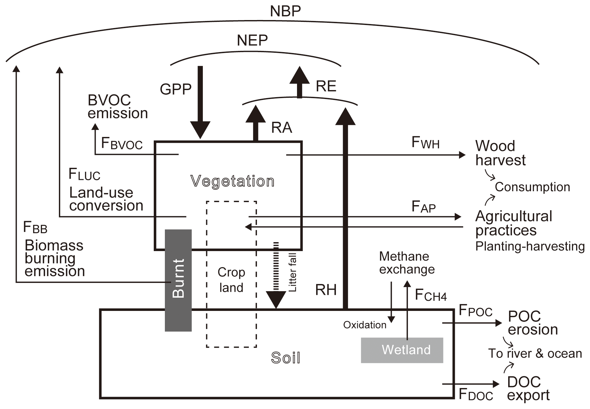
Figure 1 Schematic diagram of the carbon budget of the terrestrial ecosystem as simulated in this study. Thick lines show major carbon flows, and thin lines show minor carbon flows.

2.2.1 Land-use change (F_LUC)

Carbon emissions associated with land-use conversion were estimated for the historical period on the basis of a protocol proposed by McGuire et al. (2001), using the Land Use Harmonization (LUH) dataset (Hurtt et al., 2006). The LUH dataset provides both land-use states and their mutual transition matrix. First, the annual transition rate from primary and secondary lands to other land-use types was determined by the LUH dataset. This transition rate was multiplies by the average carbon stock in natural lands simulated by the VISIT model to estimate the amount of carbon affected by land-use conversion. This carbon was then separated into three components with different residence times from less than 1 year (detritus) to 100 years (wood products). The detritus, including dead root biomass, was transferred to the soil litter pool and then decomposed. The fractions of wood products with 10- and 100-year residence times are biome dependent (McGuire et al., 2001). Note that wood harvest not associated with land-use change (e.g., selective cutting) was separately evaluated as the F_WH term (Sect. 2.2.6). The VISIT model has been used to assess the effects of land-use change from the point scale (Adachi et al., 2011; Hirata et al., 2014) to the global scale (Kato et al., 2013; Arneth et al., 2017).

2.2.2 Biomass burning (F_BB)

Wildfire and associated biomass burning have been studied with respect to their effects on land disturbance, carbon biogeochemistry, and climatic interactions (e.g., Randerson et al., 2006; Knorr et al., 2016). The biomass burning scheme of the VISIT model has been described and evaluated by Kato et al. (2013). Biomass burning emission was calculated as follows:

$$\begin{array}{}\text{(3)}& F_{\mathrm{BB}}=\mathrm{fBurned}\times \mathrm{DC}\times \mathrm{BI}\times {\mathrm{EF}}_{\mathrm{BB}},\end{array}$$

where fBurned is the burned area fraction in natural vegetation, DC is the area-based carbon density, BI is the burned intensity (fraction of fire-affected carbon), and EF_BB is the emission factor (emission per unit burned biomass). fBurned is estimated in a prognostic manner using an empirical fire scheme originally developed by Thonicke et al. (2001) for the Lund–Potsdam–Jena dynamic global vegetation model. This scheme estimates the length of the fire season and the corresponding burned area fraction from monthly values of soil water content and fuel load. Agricultural waste burning and prescribed fires for ecosystem management are not considered here. Differences in fire susceptibility among biomes are characterized by a parameter of critical moisture content for fire ignition. DC, fuel carbon stock per area, is obtained from the VISIT simulation; it is assumed that the plant leaf, stem, root, and soil litter stocks are subject to biomass burning. BI is a biome- and stock-specific parameter obtained from Hoelzemann et al. (2004), ranging from 0.0 for humid forest root to 1.0 for forest and grassland litter. The emission factor EF_BB is also a biome- and stock-specific parameter and differs among emission substances; this study considered CO₂, carbon monoxide, black carbon, and methane. EF_BB values for each biome and stock were obtained from Hoelzemann et al. (2004). Other carbon flows associated with biomass burning, such as production and burial of charcoal, were not considered.

2.2.3 BVOC emission (F_BVOC)

Emissions of BVOCs, such as isoprene and monoterpene, attract particular attention from atmospheric chemists, and several emission schemes have been developed. Here, a convenient scheme of Guenther (1997) was incorporated into the VISIT model with a few modifications. The scheme estimates BVOC emission as follows:

$$\begin{array}{}\text{(4)}& \begin{array}{rl}{F}_{\mathrm{BVOC}}& ={\mathrm{EF}}_{\mathrm{BVOC}}\times \mathrm{FD}\times \mathrm{DL}\times \mathrm{fPPFD}\times \mathrm{fTMP}\\ & \times \mathrm{fPhenology},\end{array}\end{array}$$

where EF_BVOC is the emission factor of BVOC, FD is foliar density, DL is day length, and fPPFD, fTMP, and fPhenology are scalar coefficients for light (photosynthetic photon flux density), temperature, and phenological factors, respectively. EF_BVOC was derived from Lathiére et al. (2006) for representative species such as isoprene, monoterpene, methanol, and acetone. FD, leaf carbon stock per ground area, and DL were from the VISIT simulation. Due to the difference in biochemical pathways, only isoprene emission is responsive to light intensity (fPPFD = 0–1), while other species are insensitive (fPPFD = 1). BVOC emission increases with temperature, and fTMP differs between isoprene and other monoterpene families. fPhenology, the effect of leaf aging, differs between evergreen and deciduous vegetation. Here, based on the model simulation, leaf age distribution was modified to consider this difference explicitly; fPhenology values ranged from 0.05 for immature leaves (leaf age <1 month) to 1.2 for mature leaves (leaf age 2–10 months for deciduous and 3–24 months for evergreen leaves). Emission reduction due to leaf senescence is evaluated by decreasing fPhenology value. F_BVOC was extracted from the leaf carbon pool in the model, and impacts of released BVOCs on atmospheric chemistry and their climatic feedback were ignored.

2.2.4 Methane emission ($F_{{\mathrm{CH}}_{\mathrm{4}}}$)

Methane is a greenhouse gas second to CO₂ in importance, but here I focus on methane exchange in terms of the carbon budget. Land-surface CH₄ exchange was simulated separately for wetland (F_wetland, source) and upland (F_upland, sink) fractions within each grid cell, as described in Ito and Inatomi (2012):

$$\begin{array}{}\text{(5)}& F_{{\mathrm{CH}}_{\mathrm{4}}}=f_{\mathrm{wetland}}\times F_{\mathrm{wetland}}-\left(\mathrm{1}-f_{\mathrm{wetland}}\right)\times F_{\mathrm{upland}},\end{array}$$

where f_wetland is the wetland fraction within a grid cell. In the wetland fraction, F_wetland was simulated using a mechanistic scheme developed by Walter and Heimann (2000) that uses a multi-layer soil model and simulates gaseous methane emission by physical diffusion, ebullition, and plant-mediated transportation. The same scheme was applied to paddy fields, found mostly in Asia, using seasonal inundation by irrigation. In this study, the top 1 m of soil was divided into 20 layers, and methane gas diffusion was solved numerically with a finite-difference method including the vertical gradient of diffusivity. Microbial methane production occurs below the water table and is sensitive to moisture, temperature, and plant activities (substrate supply). It is assumed to increase exponentially with the temperature, and it stops below the freezing point. Ebullition is assumed to occur when the methane concentration exceeds 500 µmol L⁻¹. Plant-mediated transport depends on the methane concentration gradient between the atmosphere and soil layers and is strongly influenced by plant type and rooting depth. Above the water table, methane oxidation by aerobic soil is calculated as a function of soil temperature and the methane concentration of the air space. In the upland fraction such as forests and grasslands, F_upland is calculated using a semi-mechanistic scheme (Curry, 2007) that calculates methane uptake as a vertical diffusion process affected by soil porosity and microbial activity. The wetland fraction f_wetland was derived from the Global Lake and Wetland Dataset (Lehner and Döll, 2004) and was held fixed throughout the simulation period. Temporal variations in the inundation area and water table depth in the wetland fraction are key factors in estimating F_wetland. In this study, seasonal variation in the inundated area was prescribed by satellite data by microwave remote sensing (Prigent et al., 2001), and the temporal variability of water table depth was determined by the water budget estimated by the VISIT model (Ito and Inatomi, 2012). Therefore, interannual variability in inundation area, such as that due to droughts and floods, could have been underrepresented in this study.

2.2.5 Agricultural carbon flows (F_AP)

Agricultural practices, including cropping, harvesting, and consumption, are an important component in the global carbon budget (Ciais et al., 2007; Wolf et al., 2015). The VISIT model uses a simplified agriculture scheme, in which global croplands are aggregated, on the basis of physiology and cultivation practices, into three types: C₃-plant cropland (e.g., wheat), C₄-plant cropland (e.g., maize), and paddy field. The scheme assumes a single-cropping cultivation system in temperate regions, where the growing period is determined by a critical mean monthly temperature of 5 ^∘C. In tropical regions (annual mean temperature >20 ^∘C), a continuous (nonseasonal) cropping system is assumed in which planting and harvesting occur at constant rates in every month. Irrigation is not explicitly included in the model; instead the water-stress factor for cropland plants is relaxed from its value for natural vegetation. At the start of the growing period, a certain amount of carbon is added to plant biomass pools to represent planting. The crops are harvested when the surface temperature falls below the critical temperature. This study used a single value of 0.45 for the harvest index (fraction of harvested biomass); however, this index varies among crop types and regions, and the uncertainties in this parameter are considered in Sect. 4.5. Residual plant biomass was transferred to the litter pool as agricultural detritus, and this study ignored manure production and consumption processes. Harvested crops were exported from the ecosystem, and the complexities of horizontal food displacement and consumption were also ignored.

2.2.6 Wood harvest (F_WH)

Timber harvest by logging in forested lands was evaluated primarily from the LUH dataset (Hurtt et al., 2006), in which the annual wood harvest rate was derived from national data compiled by the United Nations Food and Agricultural Organization. Hurtt et al. (2006) estimated the spatial pattern of wood harvest in each country from land-use data. In this study, regrowth and carbon accumulation of forests after logging was simulated as a recovery of the carbon stock to its previous level of mature forest. As was done for crops, the harvested wood biomass was assumed to be exported from the ecosystem, specifically the stem carbon pool; horizontal transportation to and consumption in other grid cells were ignored. Note that emissions from harvested timber associated with land-use change were evaluated as part of the F_LUC term.

2.2.7 Dissolved organic carbon export (F_DOC)

Production and consumption of DOC are important processes in terrestrial ecosystems, in terms of soil formation and riverine transport (Nelson et al., 1993). In this study, the VISIT model included a simple scheme of DOC dynamics developed by Grieve (1991) and Boyer et al. (1996), in which the DOC concentration in soil water is determined by the balance of production, decay, and export. The production and decay rates are determined by soil temperature, and the export rate is determined by runoff discharge. In this study, net carbon export by DOC was extracted from the mineral soil pool. Because the VISIT model does not include a river routing scheme, DOC extraction was independently evaluated at each grid cell, and lateral transportation and decay processes were not simulated.

2.2.8 Particulate organic carbon export (F_POC)

Export of POC is assumed to occur mainly in association with soil displacement by water erosion, which can cause soil degradation. The VISIT model incorporates the Revised Universal Soil Loss Equation (Renard et al., 1997) to estimate the rate of soil displacement by water erosion (Ito, 2007). Annual displacement of soil carbon is calculated by

$$\begin{array}{}\text{(6)}& F_{\mathrm{POC}}=\mathrm{fC}\times R\times L\times S\times K\times C\times P,\end{array}$$

where fC is soil carbon content and R, L, S, K, C, and P are coefficient factors of rainfall, slope length, slope steepness, soil erodibility, vegetation coverage, and conservation practices, respectively, as described in Ito (2007). fC is obtained from the VISIT simulation, and F_POC is extracted from the soil surface litter pool. Although it was developed for management of local croplands, this practical scheme and its derivatives have been used for continental-scale studies (e.g., Yang et al., 2003; Schnitzer et al., 2013; Naipal et al., 2018). Transport of terrestrial carbon to inland waters or the ocean is, however, a complicated process (Berhe et al., 2018); for example, large fractions of displaced soil are redistributed in riverbanks, lake shores, and estuaries. The fate of eroded carbon is assumed to be 20 % in CO₂ evasion by decomposition, 60 % in sedimentation, and 20 % in export to lakes and oceans (Lal, 2003; Kirkels et al., 2014). The export fraction is highly uncertain and is discussed further in the parameter uncertainty analysis of Sect. 4.5.

2.3 Simulations and analyses

Global simulations were conducted from 1901 to 2016 at a spatial resolution of $\mathrm{0.5}{}^{\circ }\times \mathrm{0.5}{}^{\circ }$ in latitude and longitude. The VISIT model was applied to each grid cell, and lateral interactions such as riverine transport, food and timber export, and animal migration were ignored. To obtain the initial stable carbon balance, a spin-up calculation under stationary conditions was conducted for each grid cell for 300 to 3000 years, depending on climate conditions and the biome type. This section describes sensitivity simulations to analyze the impacts of different forcing variables, ensemble perturbation simulations to assess the effect of parameter uncertainty, and several supplementary simulations.

All simulations used climate conditions from CRU TS 3.25 (Harris et al., 2014), consisting of monthly temperature, precipitation, vapor pressure, and cloudiness. The historical change in atmospheric CO₂ concentration was taken from observations (e.g., Keeling et al., 2009). The global distribution of natural vegetation was determined by Ramankutty and Foley (1998) for potential vegetation types and Olson et al. (1983) for actual vegetation types. This study classified natural vegetation into 28 types after Olson et al. (1983). Historical land-use status, transitional changes, and wood harvest in each grid cell were derived from the LUH data (Sect. 2.2.1). Until 2005, land-use data were compiled on the basis of statistics and various ancillary data, and after 2006 the data were extended by using an intermediate projection scenario (RCP4.5) produced with an integrated assessment model. The distribution of dominant crop types was determined from the global dataset of Monfreda et al. (2008) and used to calculate F_AP and $F_{{\mathrm{CH}}_{\mathrm{4}}}$ (for paddy field). For the calculation of $F_{{\mathrm{CH}}_{\mathrm{4}}}$, the wetland fraction in each grid cell was determined from the GLWD (Global Lake and Wetland Dataset) (Sect. 2.2.4). For the estimation of F_POC, slope factors (L and K) were calculated from the GTOPO30 topography data (https://doi.org/10.5066/F7DF6PQS; USGS, 1996), and the erodibility factor (S) was calculated from soil composition data (Reynolds et al., 1999). Vegetation coverage (C) and conservation practice (P) factors were determined from the dominant natural vegetation and cropland types, also considering the difference in management intensity between developed and developing countries.

This study focused on the carbon budget of terrestrial ecosystems and analyzed the following variables: GPP, RE, NEP, NBP, biomass carbon stock, and soil carbon stock. The mean residence time (MRT) of the biomass, soil, and total ecosystem carbon stocks at transitional states were approximately calculated in a similar manner to Carvalhais et al. (2014):

$$\begin{array}{}\text{(7)}& \mathrm{MRT}=\mathrm{C}\mathrm{stock}/\mathrm{flux},\end{array}$$

where flux is net primary production (NPP) for biomass (= GPP − RA), RH for soil, and the sum of these fluxes (NPP + RH) for the total ecosystem carbon stock.

2.3.1 Sensitivity simulations

To evaluate and separate the effects of MCFs, 12 simulation experiments were conducted:

• EX0: no MCF was included, and the terrestrial carbon budget was determined by GPP, RA, and RH, such that NBP was identical to NEP.

• EX_LUC: only F_LUC was added to EX0.

• EX_BB: only F_BB was added to EX0.

• EX_BVOC: only F_BVOC was added to EX0.

• EX${}_{{\mathrm{CH}}_{\mathrm{4}}}$: only $F_{{\mathrm{CH}}_{\mathrm{4}}}$ was added to EX0.

• EX_AP: only F_AP was added to EX0.

• EX_WH: only F_WH was added to EX0.

• EX_DOC: only F_DOC was added to EX0.

• EX_POC: only F_POC was added to EX0.

• EX_ALL: all eight MCFs were considered, equivalent to the baseline simulation.

• EX_BGC: biogeochemical flows (F_BVOC, $F_{{\mathrm{CH}}_{\mathrm{4}}}$, F_DOC, and F_POC) were added to EX0.

• EX_ATP: anthropogenic (human-dominated) flows (F_LUC, F_BB, F_AP, and F_HW) were added to EX0.

The differences between EX0 and the next eight simulations indicate the effects of individual MCFs, and the difference between EX_ALL and EX0 shows the combined effect of these MCFs. Interactions among the MCFs through changes in the terrestrial carbon stock may mean that their effects are not linearly additive. For example, land-use changes have indirect impacts on biomass burning, BVOC emission, and water erosion (e.g., Nadeu et al., 2015). Also, the inclusion of the MCFs affects the major flows of primary production and respiration. For example, BVOC emission reduces the carbon stored in leaves, which leads to reductions in light absorption and GPP. In croplands, planting and harvest substantially influence GPP and respiration. The last two simulations (EX_BGC and EX_ATP) sought to evaluate the relative contributions of what are conventionally considered biogeochemical and human-affected processes.

2.3.2 Parameter-ensemble simulations

Large uncertainties remain in the estimates for each MCF and its impacts. These uncertainties can emerge among different models, forcing data, and parameters, and evaluating them is important but difficult. The schemes used in this study include empirical formulations and parameters, some of which are not well constrained by observational data. Upscaling locally adapted schemes and parameters can lead to biased results at the global scale. To characterize the range of uncertainty caused by poorly determined parameters, I conducted a set of ensemble simulations, based on EX_ALL, in which the values of the following representative parameters of the eight MCFs were randomly perturbated at the same time: annual deforestation rate in F_LUC, biomass burning emission factors in F_BB, BVOC emission factors in F_BVOC, wood harvest rate in F_WH, crop harvest index in F_AP, methane production and oxidation potentials in $F_{{\mathrm{CH}}_{\mathrm{4}}}$, DOC export rate in F_DOC, and erodibility and land-export fraction in F_POC. It should be noted here that other parameters have their own uncertainties and that this study focused on these eight representative parameters for explanatory purposes. Also, these uncertainties may increase as they incorporate the differences among models with differing structures and assumptions. A total of 146 ensemble simulations were conducted (Fig. S2) in which these parameters were perturbed by randomly selecting values from the Gaussian distribution within the range of ±30 %. All other configurations were those of EX_ALL. Means, medians, and 95 % confidence intervals were calculated from the 146 resulting terrestrial carbon budgets.

2.3.3 Supplementary simulations

To further investigate the characteristics and influence of MCFs, five supplementary simulations were conducted. In the first, based on the protocol of EX_ALL, land-use status was held fixed at its initial state in 1901 (EX_fxLUC). This simulation differs from EX_LUC by also removing the effects of land-use change on F_AP and F_POC from alterations in cropland area. In the second, the climate condition was held fixed at its initial state in 1901 (EX_fxCL). This simulation removed the effect of temperature and precipitation changes on MCFs and the terrestrial carbon budget. Many carbon flows, including the major ones (GPP, RA, and RH) as well as minor ones (F_BB, F_BVOC, $F_{{\mathrm{CH}}_{\mathrm{4}}}$, F_AP, F_DOC, and F_POC), are more or less influenced by climate conditions. In the third simulation, atmospheric CO₂ concentration was held fixed at its level in 1901 (EX${}_{{\mathrm{fxCO}}_{\mathrm{2}}}$). Although no MCFs are directly sensitive to ambient CO₂ conditions, the fertilization effect of rising CO₂ concentration affects GPP and related carbon dynamics, including MCFs.

The fourth and fifth simulations focused on biomass burning. As explained earlier, the fire scheme in the VISIT model does not explicitly consider human activities such as prescribed fires and fire prevention, probably leading to biases in burned area and subsequent emission patterns. For example, the fire scheme poorly captures the recent declining trend in burned area (Andela et al., 2017) due to human suppression. These two simulations used satellite remote-sensing data to evaluate the effect of model-estimated burned area. In the fourth simulation, based on EX_ALL, interannual variability in burned area was prescribed by the Global Fire Emission Database 4s (GFED4s) remote-sensing product (Randerson et al., 2012) during the period 1998–2016 (EX_BB1). In the fifth simulation (EX_BB2), the simulated mean burned area for 1901–2016 was adjusted with respect to GFED4s. For example, if the control run (EX_ALL) had estimated burned areas that averaged 20 % higher than GFED4s, an adjustment coefficient of 100∕120 would have been applied to the burned area simulated in this run to remove the systematic overestimation.

3 Results

3.1 Global terrestrial carbon budgets

The mean annual global terrestrial GPP in 1990–2013 (a period when comparative estimates were available) was simulated as 144.0±4.4 Pg C yr⁻¹ in EX0 and 125.4±4.0 Pg C yr⁻¹ in EX_ALL (mean ± standard deviation of interannual variability). Ecosystem respiration (RE) was simulated as 141.0±3.6 Pg C yr⁻¹ in EX0 and 118.8±3.2 Pg C yr⁻¹ in EX_ALL. Mean vegetation and soil carbon storage differed in the two simulations: EX0 produced 648 Pg C in vegetation and 1560 Pg C in soil organic matter, and EX_ALL produced 477 Pg C in vegetation and 1290 Pg C in soil organic matter. The mean annual net CO₂ budget determined by the major flows, NEP (= GPP − RE), was simulated as 2.99±1.18 Pg C yr⁻¹ in EX0 (which ignores MCFs) and 6.57±1.07 Pg C yr⁻¹ in EX_ALL. Because both simulations used the same climate, atmospheric CO₂, and land-use data, these differences – lower carbon stocks, smaller GPP and RE flows, and a large sink by NEP – are attributable to the inclusion of the MCFs.

The individual MCFs had different impacts on the global terrestrial carbon budget. For the vegetation carbon stock, impacts were negligible (<1 Pg C) from methane emission, DOC and POC exports by water movement, and agricultural practices, whereas impacts were substantial from land-use change (−88.5 Pg C), biomass burning (−46.4 Pg C), wood harvest (−28.5 Pg C), and BVOC emission (−24.2 Pg C). For the soil carbon stock, the two largest negative impacts were from land-use change (−108 Pg C) and biomass burning (−71.2 Pg C). Interestingly, the inclusion of BVOC emission reduced the soil carbon stock (−18.1 Pg C) through the loss of photosynthate carbon and decreased carbon supply to the soil. The inclusion of agricultural carbon flows (planting and harvesting, other than land-use change) decreased the soil carbon stock (−55.6 Pg C), although planting enhanced vegetation productivity and carbon supply to the soil. The inclusion of DOC and POC exports moderately reduced the soil carbon stock (−5.9 and −3.6 Pg C, respectively).

Most of the difference in GPP between EX0 and EX_ALL was attributable to land-use change (−12.8 Pg C yr⁻¹), wood harvest (−0.9 Pg C yr⁻¹), and BVOC emission (−0.9 Pg C yr⁻¹). Biomass burning, though it has substantial impacts on biomass, also slightly decreased GPP (−0.75 Pg C yr⁻¹). The simulated impacts of MCFs on RE were mostly similar to those for GPP. The relatively high NEP in EX_ALL was largely attributable to compensatory regrowth in response to biomass burning (2.03 Pg C yr⁻¹), BVOC emission (0.69 Pg C yr⁻¹), and wood harvest (0.41 Pg C yr⁻¹).

Human activities (EX_ATP) had greater impacts on terrestrial carbon stocks than biogeochemical processes (EX_BGC), as mean ecosystem carbon stock decreased by 172 Pg C in EX_BGC and 296 Pg C in EX_ATP. The sum of these two depressions in carbon stock, 467 Pg C, was larger than that estimated in the all-inclusive experiment (EX_ALL), 440 Pg C, which points to nonlinear offsetting effects among the MCFs.

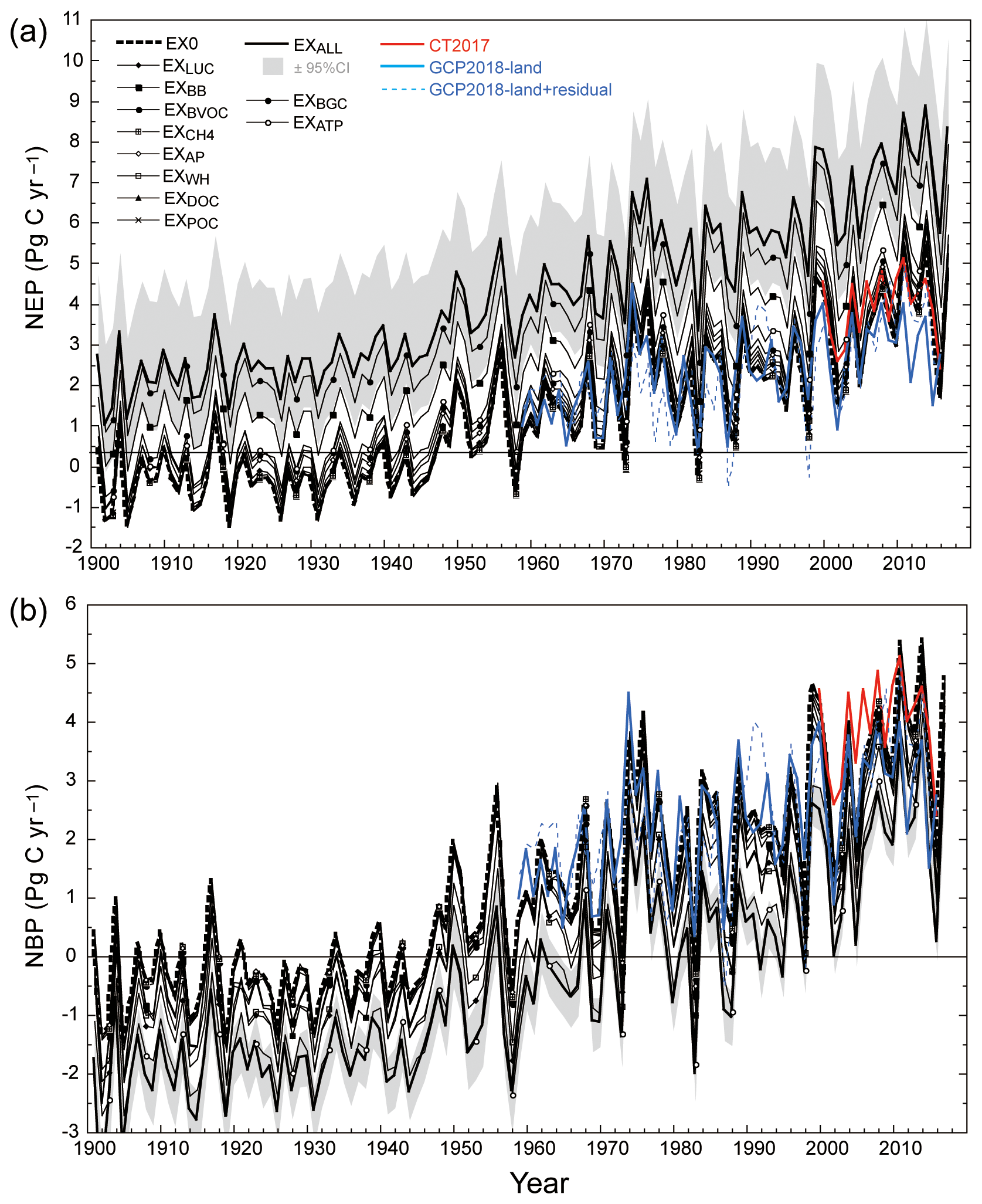
Figure 2 Temporal changes in the simulated global terrestrial carbon budget from this study (black lines), CarbonTracker 2017 (CT2017; Peters et al., 2007; red lines), and the Global Carbon Project (GCP; blue lines). (a) NEP and (b) NBP. See the text for the simulation experiments. Figure S3 presents extracted results for the period 1980–2016.

The carbon budget including the MCFs (NBP) in 1990–2013 was estimated as 1.36±1.12 Pg C yr⁻¹ of net sink in EX_ALL, that is, 20.7 % of NEP (see Table 1 for decadal summary). Figure 2 shows the temporal change in global annual NEPs and NBPs in each experiment for the 1901–2016 study period (see Fig. S3 for details of the 1990–2013 period). The inclusion of MCFs considerably altered the mean state of the terrestrial carbon budget throughout the simulation period. Little difference was found among the experiments in interannual variability and decadal trends. For example, linear trends of NBP in 1980–2013 were estimated as (0.0783 Pg C yr⁻¹) yr⁻¹ in EX0 and (0.0890 Pg C yr⁻¹) yr⁻¹ in EX_ALL. Interestingly, the larger differences among experiments for NEP (±1.15 Pg C yr⁻¹, standard deviation among EX0 to EX_ALL) than for NBP (±0.52 Pg C yr⁻¹) indicated a convergence of estimated carbon budgets after including MCFs.

Table 1 Decadal summary of simulation results of net global terrestrial carbon budget (Pg C yr⁻¹).

NEP, net ecosystem production; NBP, net biome production. Model designations are defined in the text.

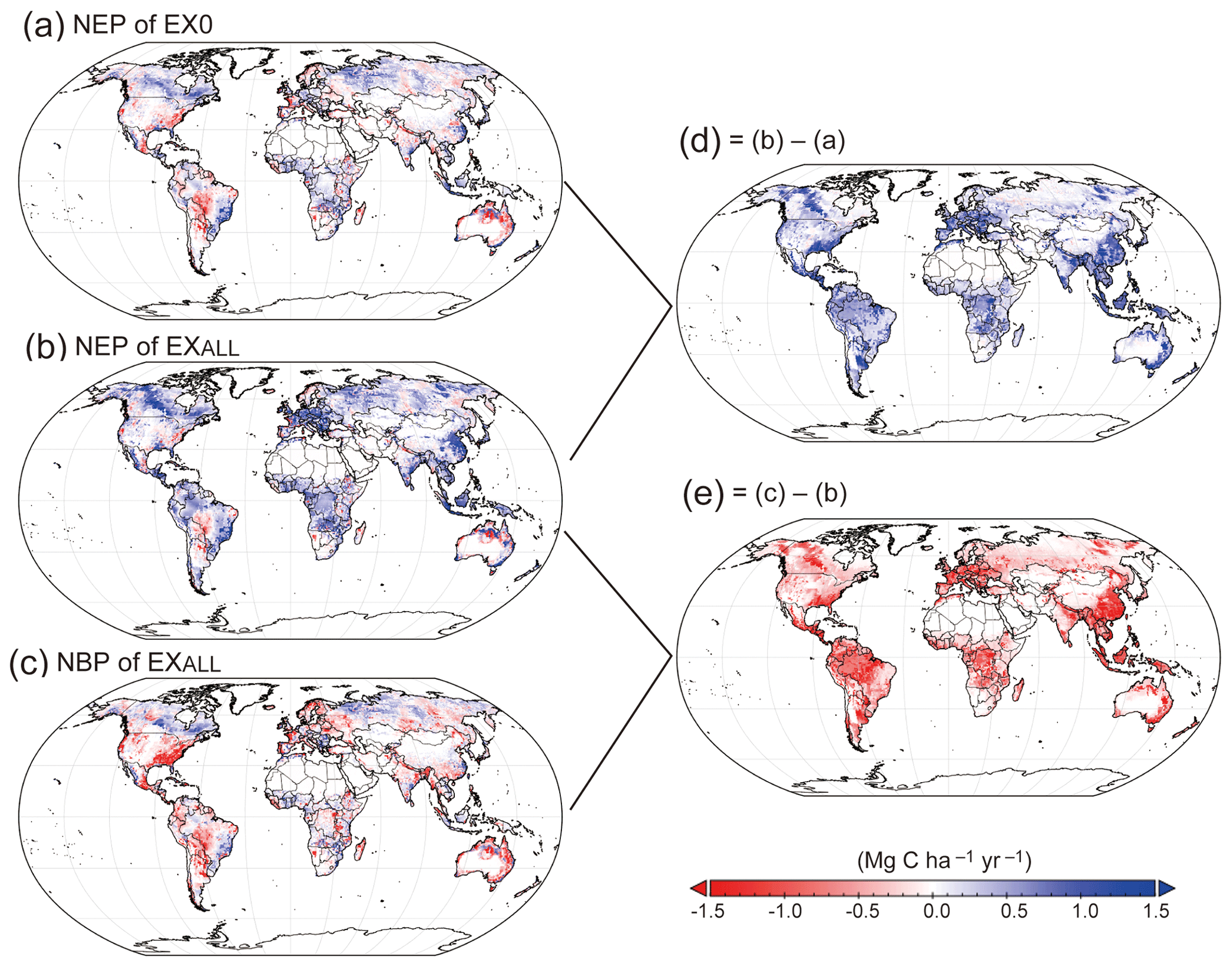
Figure 3 Global distribution of simulated terrestrial carbon budget in the 2000s. (a) NEP in EX0, (b) NEP in EX_ALL, (c) NBP in EX_ALL, (d) difference between panels (b) and (a) showing the apparent effects of MCFs on NEP, and (e) difference between panels (c) and (b) showing the apparent effects of MCFs on NBP.

The spatial distribution of carbon budgets shows that EX0 identified a vast area of tropical, temperate, and boreal forests as moderate net carbon sinks (Fig. 3a). The inclusion of MCFs in EX_ALL (Fig. 3b) intensified this net sink in tropical forests and parts of the temperate and boreal forests, but it decreased NEP in grasslands and pastures in central North America and Europe, turning parts of them into net carbon sources (Fig. 3d). The spatial distribution of NBP in EX_ALL (Fig. 3c) was a heterogeneous pattern of sink and source. Several tropical and subtropical forests had negative NBP, although NEP in these areas was estimated as positive or neutral. As shown in Fig. 3e, with the addition of MCFs, a large part of the terrestrial ecosystem was simulated to lose carbon. The contributions of each flow are described in the next section.

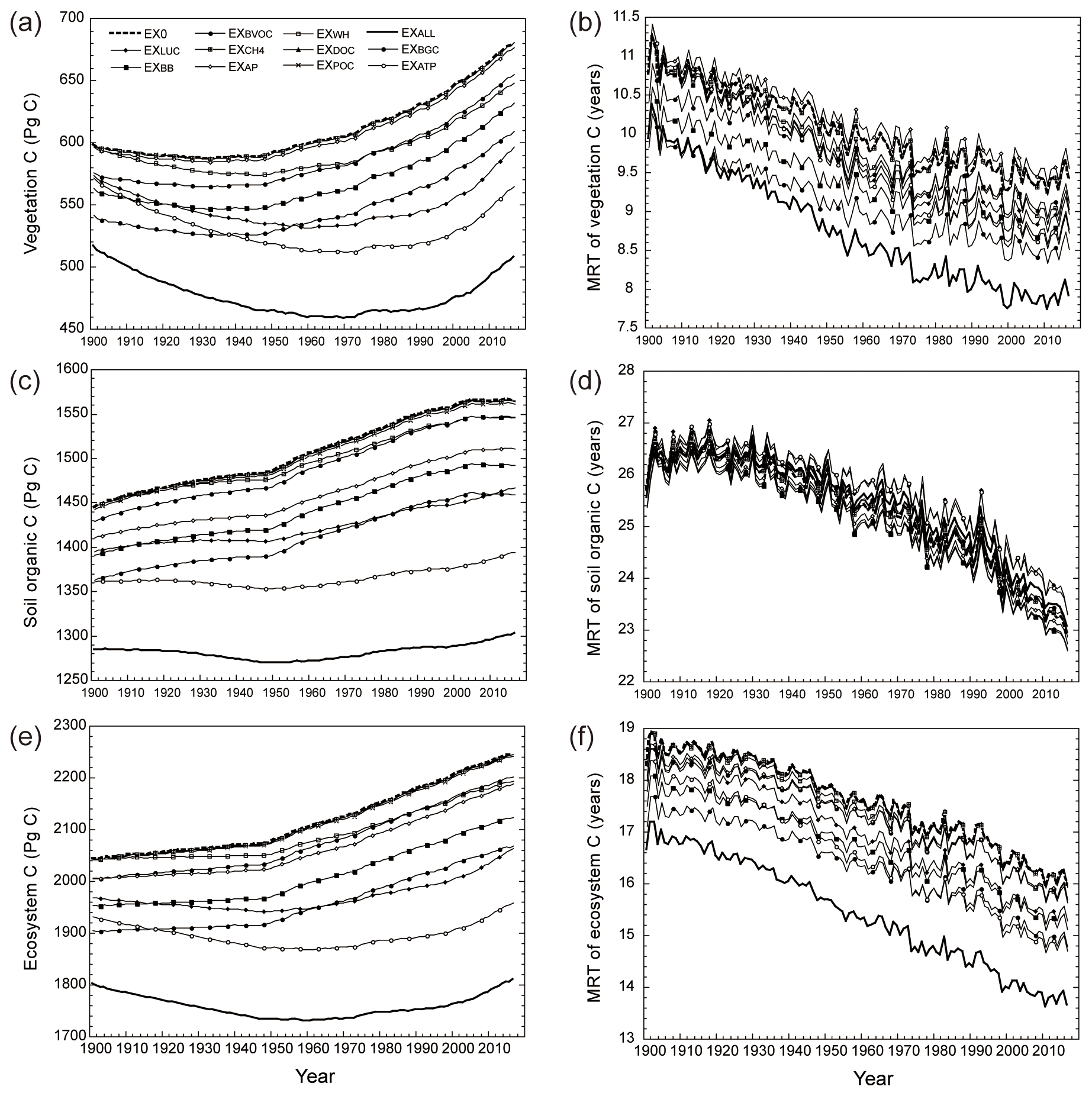
Figure 4 Time series of simulated carbon stocks and their mean residence time (MRT) in different experiments. (a) Vegetation biomass and (b) its MRT, (c) soil organic carbon and (d) its MRT, and (e) total ecosystem carbon stock and (f) its MRT.

The decrease in carbon stocks in terrestrial ecosystems after the addition of MCFs indicates that the mean residence time (MRT) of these stocks became shorter than would be estimated solely from major carbon flows (see Fig. S4 for the spatial distribution of stocks and MRTs). As shown in Fig. 4, simulated terrestrial carbon stocks in EX_ALL were steady or slightly declining until around 1960, especially when land-use change (e.g., tropical deforestation) was included. After 1960, carbon stocks in vegetation and soil began to gradually increase. As described earlier, the simulated carbon stocks differed among the experiments by as much as 440 Pg C as a consequence of including MCFs. Also, the inclusion of MCFs made large impacts on GPP and RE (Fig. S5) by altering vegetation structure and soil carbon storage. Simulated MRTs grew clearly shorter (i.e., turnover was accelerated), as a result of global changes such as temperature rise enhancing respiratory emissions. Note that MRTs also grew shorter in the result of EX0, which ignored MCFs, but including the MCFs increased the difference in MRT among the experiments. For example, the difference in MRT of vegetation biomass between EX0 and EX_ALL grew from 0.89 years in the 1900s to 1.54 years in the 2000s, and the difference for soil carbon stock grew from 0.10 years in the 1900s to 0.24 years in the 2000s. The definition of MRT (Eq. 7) means that shortened MRTs could result from increases in NPP and respiration.

3.2 Simulated patterns of MCFs

Figure 5 shows the temporal changes in the eight simulated MCFs in their individual sensitivity simulations (EX_LUC to EX_POC) as well as the EX_ALL simulation. The emissions associated with land-use change (F_LUC) peaked around the 1950s at 1.2–1.4 Pg C yr⁻¹ and then gradually decreased. Biomass burning emission (F_BB) remained around 1 Pg C yr⁻¹ until the 1970s and then increased slightly to 1.5 Pg C yr⁻¹, with a large interannual variability. BVOC emission (F_BVOC) increased gradually from 0.5 Pg C yr⁻¹ in the early 20th century to 0.6 Pg C yr⁻¹ in the 21st century. Methane emission ($F_{{\mathrm{CH}}_{\mathrm{4}}}$) gradually increased from 0.11 Pg C yr⁻¹ in the first decades of the 1900s to 0.13 Pg C yr⁻¹ in the 2000s (representing 160–170 Tg CH₄ yr⁻¹). Wood harvest (F_WH) likewise increased from 0.5 Pg C yr⁻¹ in the 1900s to 1.1 Pg C yr⁻¹ in the 2000s, as did POC export by water erosion (F_POC), which increased from 0.55 Pg C yr⁻¹ in the 1900s to 0.95 Pg C yr⁻¹ in the 2000s. Crop planting and harvest (F_AP) had a mixed effect on the terrestrial carbon budget because planting enhances productivity, whereas harvesting is a direct carbon loss. As a result, F_AP had both negative (net uptake) and positive (net emission) values. DOC export (F_DOC) remained steady at around 0.14±0.004 Pg C yr⁻¹ throughout the simulation period.

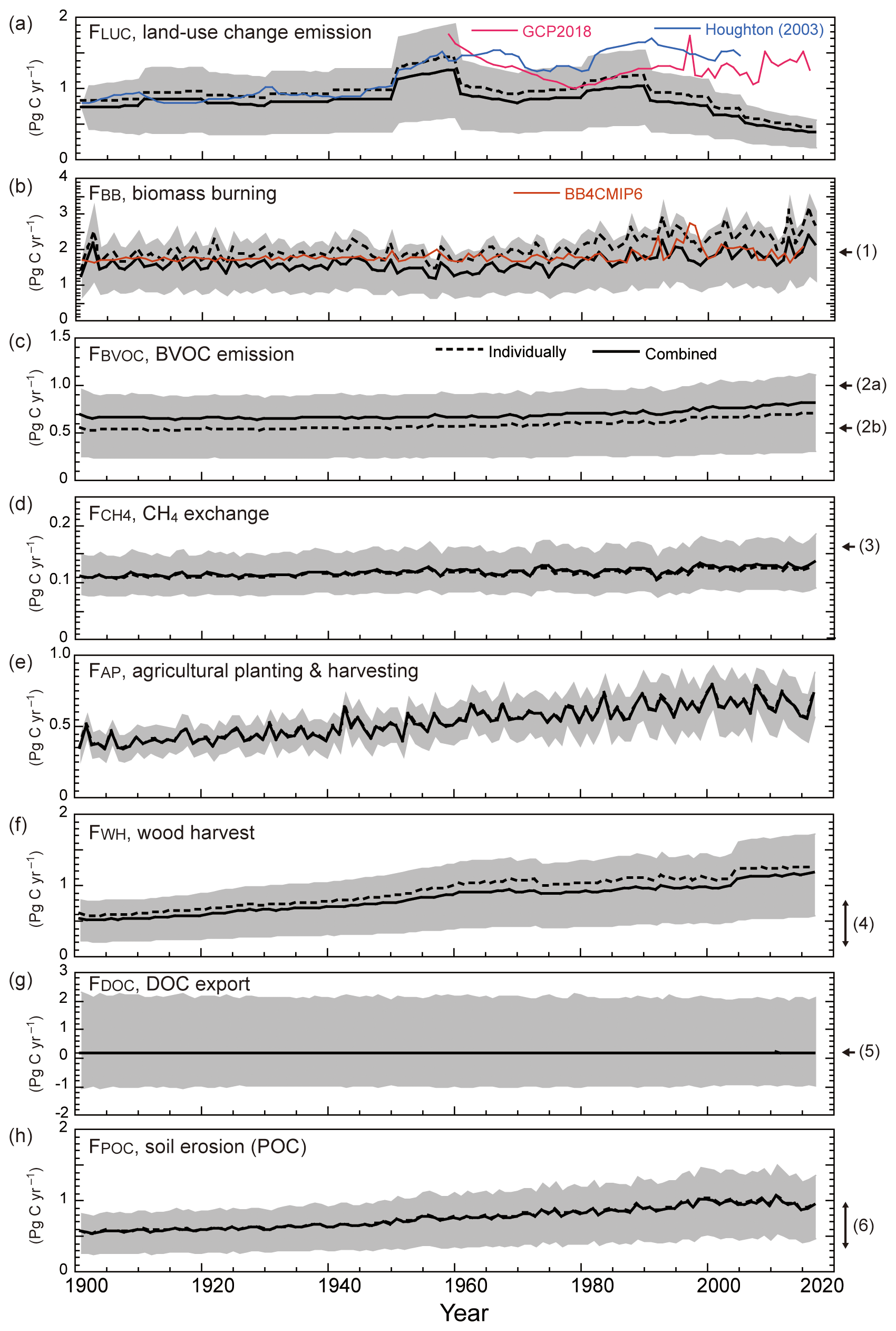
Figure 5 Time series of minor carbon flows simulated by the VISIT model and previous studies. Dashed lines are results of individually simulated flows, and solid lines are results of the EX_ALL simulated, and shading shows the 95 % confidence interval for the EX_ALL result obtained from ensemble simulations (Fig. S2). Blue and red lines in panel (a) show data of the Global Carbon Project (GCP2018) and Houghton (2003). The orange line in panel (b) shows data of BB4CMIP6 (van Marle et al., 2017). Arrows indicate the values of (1) biomass burning emission by Randerson et al. (2012), (2a) total BVOC and (2b) isoprene emissions by Guenther et al. (2012), (3) wetland and paddy methane emission by Saunois et al. (2017), (4) wood harvest by Arneth et al. (2017), (5) DOC export by Dai et al. (2012), and (6) soil erosion by Chappell et al. (2016).

The supplementary simulations showed that temporal changes in the MCFs were caused by different forcing factors. For example, when the atmospheric CO₂ concentration was fixed at its level in 1901 (EX${}_{{\mathrm{fxCO}}_{\mathrm{2}}}$, data not shown), the increasing trend in F_BVOC (Fig. 5c) nearly vanished, whereas other flows such as F_WH and F_POC were insensitive to CO₂. When climate conditions were held fixed (EX_fxCL), F_BB showed only a decadal trend in response to changes in fuel load, and climate-induced interannual variability in burned area and fire-induced emissions (Fig. 5b) disappeared.

Figure 6 Global distribution of the simulated MCFs (plus crop harvest) in 2000–2009. Results of EX_ALL are shown.

The MCFs considered in this study showed distinct spatial patterns (Fig. 6). F_LUC occurred mainly in the tropical forests of South America, Africa, and South Asia. F_BB occurred in subtropical areas in Africa, tropical forests in South America and Southeast Asia, the Mediterranean area, and boreal forests in North America and east Siberia. F_BVOC was highest in tropical forests and elevated in other forested areas. For $F_{{\mathrm{CH}}_{\mathrm{4}}}$, major sources included monsoon-affected parts of Asia dominated by paddy fields, tropical wetlands including floodplains of big rivers, and northern wetlands, whereas other uplands were weak sinks. For F_AP, croplands in Europe, East Asia, and North America exported large amounts of carbon (see Fig. 6f for the crop harvesting effect alone). F_WH occurred mainly in tropical forests in southern East Asia, South America, and southern North America. F_POC occurred mainly in humid and steep areas such as mountainous regions of monsoon Asia and cultivated areas. F_DOC occurred mainly in warm and humid areas such as tropical forests in South America, Africa, and Southeast Asia.

3.3 Effects of MCFs on the carbon budget

The effects of the eight studied MCFs on the global carbon budget, resulting in a lower net sink by NBP than by NEP, were dominated by five MCFs: biomass burning (F_BB), wood harvest (F_WH), POC export by water erosion (F_POC), BVOC emission (F_BVOC), and emission caused by land-use change (F_LUC) (Fig. 7a). The contributions of MCFs differed among regions. F_AP and F_BB had dominant effects in Europe (Fig. 7b) and North America (Fig. 7g), where the effects of F_LUC and F_DOC were negligible. In Africa (Fig. 7c), South America (Fig. 7h), and the global tropics (Fig. 7i), all five MCFs had similar effects. In Asia (Fig. 7e), F_POC and F_AP had the largest effects, and $F_{{\mathrm{CH}}_{\mathrm{4}}}$ emissions from the vast area of paddy fields were considerable. In semiarid regions (Fig. 7j), F_AP and F_BB were the largest.

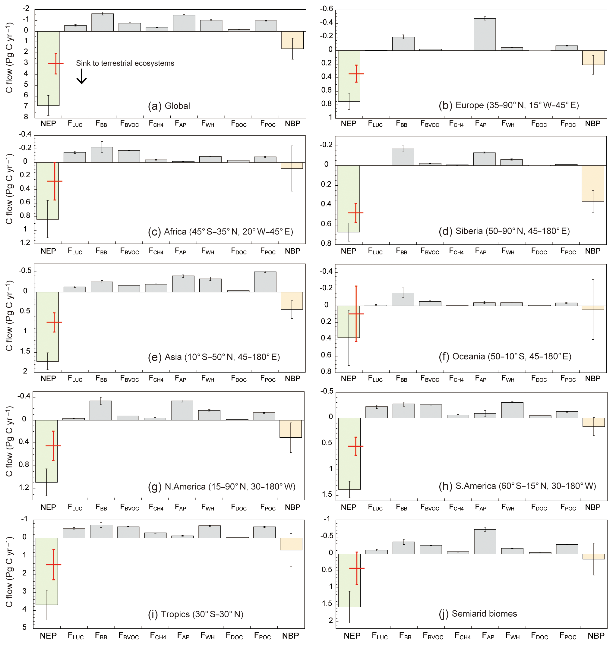
Figure 7 Regional portions of the terrestrial carbon budget in 2000–2009. Columns show the mean results of EX_ALL and error bars show the standard deviation of interannual variability. Red lines show the mean and standard deviation of NEP in EX0. Note the differences in vertical scale.

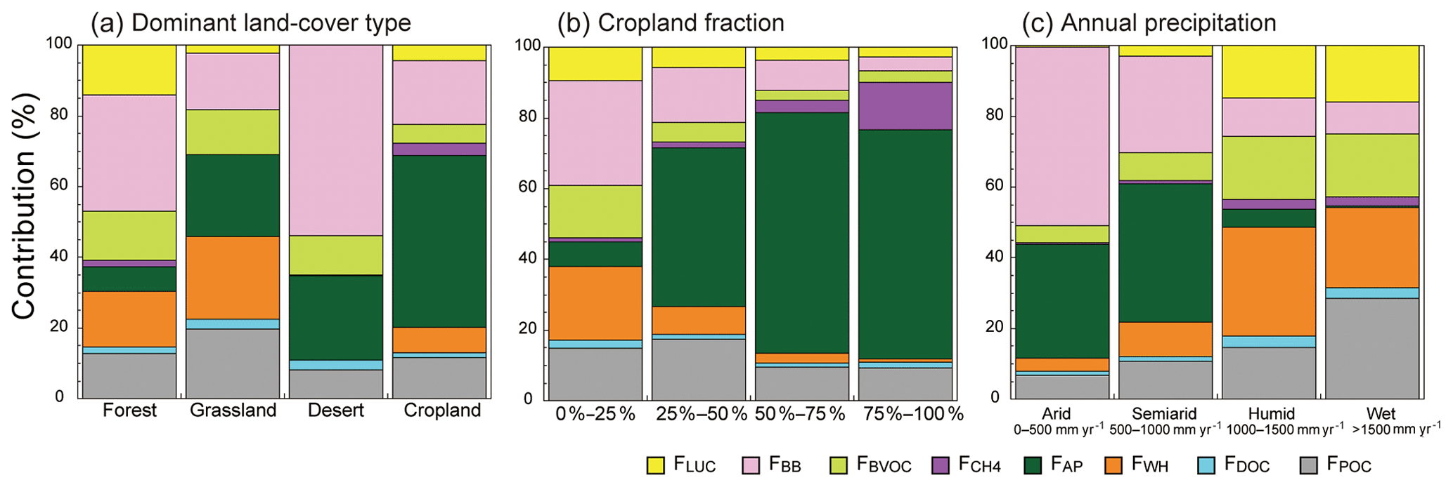
Figure 8 Relative contribution of MCFs to the terrestrial carbon budget simulated by EX_ALL in 2000–2009: (a) aggregated by dominant land-cover type, (b) aggregated by cropland fraction within grid cells, and (c) aggregated by annual precipitation.

Certain spatial tendencies become clearer in a global aggregation of the simulated results (Fig. 8) related to the dominant land-cover type in each grid cell, the cropland fraction, and aridity represented by annual precipitation. In forest-dominated grid cells (Fig. 8a), F_BB made the largest (>30 %) contribution, followed by F_WH, F_BVOC, and F_LUC, and in cropland-dominated cells, about half of the influence of MCFs was due to agricultural practices (F_AP). Because grassland-dominated cells contain fractions of woodland and cropland, F_AP and F_WH as well as F_POC made contributions in these cells. In desert-dominated cells, F_BB made up the majority of the contributions. In cells with small fractions of cropland including tropical forests (Fig. 8b), F_WH, F_BB, and F_BVOC made strong contributions, whereas in cells dominated by crops, $F_{{\mathrm{CH}}_{\mathrm{4}}}$ made a substantial contribution reflecting the vast area of paddy fields in Asia. F_POC made large contributions at all cultivation intensities, but particularly in moderately cultivated areas. An analysis based on precipitation was also informative (Fig. 8c). In arid areas (annual precipitation <500 mm), F_BB had the largest impacts, as expected from the dominance of fire-prone ecosystems such as boreal forests and subtropical woodlands. In wet areas (precipitation >1500 mm), F_LUC and F_POC made large contributions, and F_BB had a minor effect. The influence of F_WH was strongest in moderately humid to wet areas.

4 Discussion and conclusions

4.1 Comparison with previous carbon studies

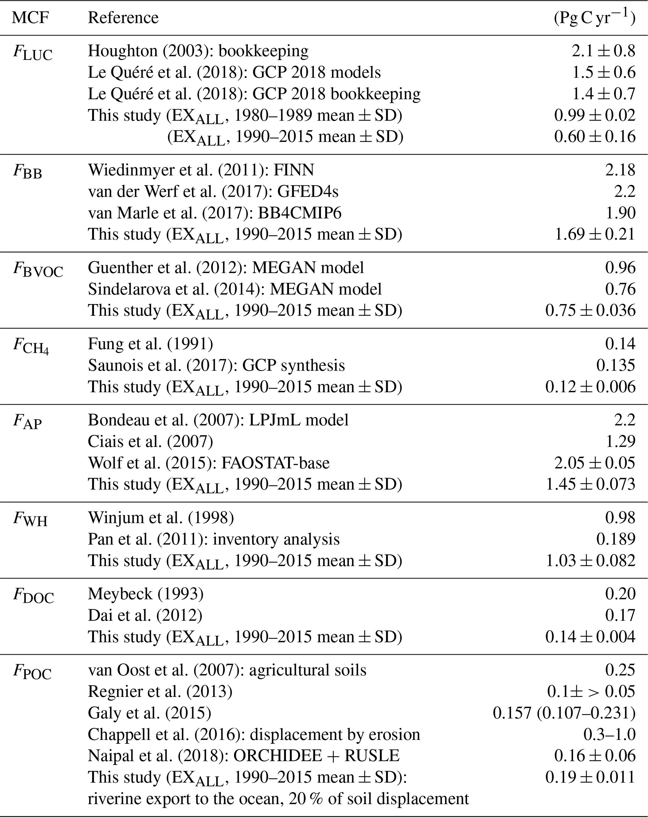
This study showed that MCFs have notable impacts on the terrestrial carbon budget; they disequilibrate ecosystem carbon stocks and affect MRTs. Most of the simulated magnitudes of MCFs were comparable to results of previous studies (Fig. 5 and Table 2), and their impacts on the carbon budget were consistent with other model studies (e.g., Yue et al., 2015; Naipal et al., 2018). In terms of F_LUC, the model estimated clearly lower emissions than the Global Carbon Project (GCP) synthesis (Le Quéré et al., 2018) and other studies, surely because this study did not use actual land-use data after 2005. Updated data would likely improve the VISIT model's performance. The fact that the simulated F_BB was slightly low compared to previous estimates implies that there is a need to refine the fire module in the model (discussed further in Sect. 4.5). The simulated F_POC was comparable to results in other studies, but there remain inconsistencies in the fate terms (riverine transport, burial, and CO₂ evasion) and the ratio of ocean and inland water export. Similarly, the simulated F_AP and F_WH appear comparable to results in other studies, but this study largely ignored their transport and consumption. Further detailed comparisons and comprehensive assessments are clearly required.

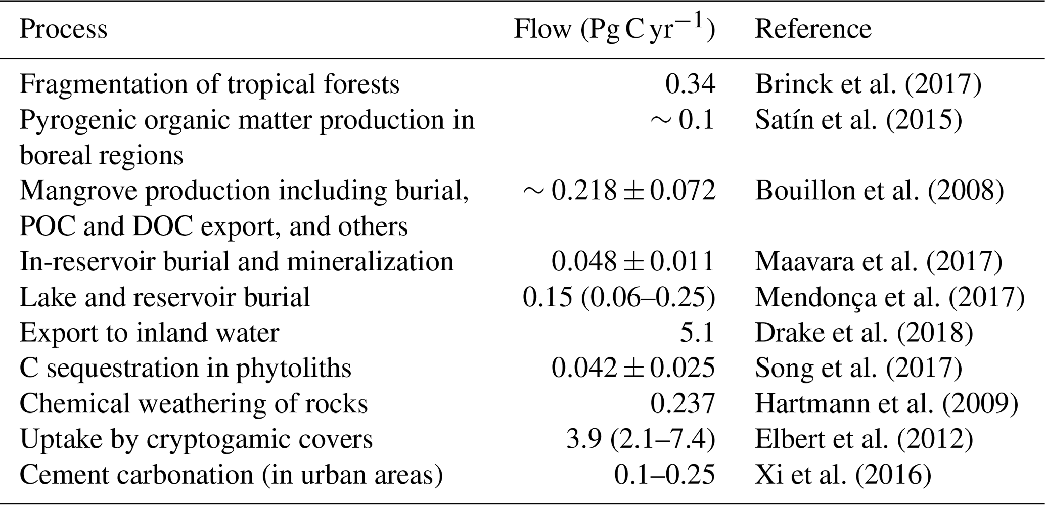
Table 2 Summary of previous estimates of minor carbon flows (MCFs).

Most models have been calibrated and validated with observational data of major carbon flows (e.g., GPP, RE, and NEP) and carbon stocks. Although recent models have begun to take account of land-use change and biomass burning, most still ignore the contributions of many other minor flows. The global GPP simulated in this study is similar to a satellite-based product of the Breathing Earth System Simulator (BESS) of Jiang and Ryu (2016): for the 2001–2013 period, the coefficient of determination (R²) was 0.77 for EX0 and 0.71 for EX_ALL (Fig. S5). All three simulations show increasing trends. In contrast, the upscaled flux measurement data of FLUXCOM (Tramontana et al., 2016) and the MOD15 satellite product (Zhao et al., 2006) show smaller interannual variability and trends, and they were only weakly correlated with the VISIT simulations (R²=0.21–0.39). Compared with the terrestrial carbon budget in the integrated synthesis of the GCP for 1959–2016 (Le Quéré et al., 2018), the simulated NEP in EX_ALL was much higher in the same period: 5.7 Pg C yr⁻¹ in EX_ALL and 2.1 Pg C yr⁻¹ in GCP. Removing the land-use emission of 1.3 Pg C yr⁻¹ would reduce the provisional NBP from GCP to 0.85 Pg C yr⁻¹, putting it closer to the simulated NBP in EX_ALL (0.68 Pg C yr⁻¹) than to the NBP in EX0 (2.33 Pg C yr⁻¹). (Figures S6 and S7 compare the results of NEP and F_LUC from the individual models in the GCP synthesis.) EX_ALL successfully captured the large aboveground vegetation biomass stock in the tropics and the small stock in boreal zones seen in observations (Fig. S8a). A similar comparison of soil carbon (Fig. S8b) also indicates the model's ability to capture the spatial gradient in this stock; an overestimation in the northern midlatitudes (around 30^∘ N) is attributable to high soil carbon accumulation in the Tibetan Plateau simulated by the model in frigid regions. It is not clear, however, whether EX_ALL (with MCFs) captured the global patterns with greater accuracy than EX0 (without MCFs), because observational datasets show considerable discrepancies, and the differences between the model simulations were relatively small. The estimated MRT of the ecosystem carbon stock in EX_ALL (14–17 years) was shorter than the MRT of 23 years (95 % confidence interval, 18–29 years) found by the data-oriented study of Carvalhais et al. (2014). This difference is attributable to the high soil carbon stock in the latter study (2397 Pg C) rather than to differences in the vegetation carbon stock and flows; both studies had similar spatial patterns of MRT.

Considering the remaining uncertainties in observational terrestrial carbon accounting, it is still difficult to perform a conclusive validation. Nevertheless, this study demonstrated the possibility of integrating various carbon flows into a single model framework.

4.2 Impacts of MCFs on regional and global carbon budgets

The simulated MCFs affect the amount of the terrestrial carbon stock by as much as 440 Pg C. The size of this difference is comparable to differences, or the model estimation uncertainty, found among biome models (e.g., Friend et al., 2014; Tian et al., 2015). By definition, NBP including the effect of MCFs is likely to correspond closely to carbon stock change as well as carbon budgets obtained by atmospheric inversions. MCFs affect the carbon budget in two major ways: first by their instantaneous carbon exports and second by the ensuing carbon uptake during recovery from these disturbances, which occurs with time lags of decadal to centennial scale, depending on the types of disturbance and their intensities (e.g., Fu et al., 2017). Assessments of MCFs would help characterize the “missing sink”, which is now primarily ascribed to terrestrial carbon uptake (Houghton et al., 1998; Le Quéré et al., 2018) by mechanisms that are still arguable. Although previous studies (e.g., Jung et al., 2011; Zscheischler et al., 2017) have noted the potential importance of MCFs and the difference between NEP and NBP (or corresponding metrics such as the net ecosystem carbon balance of Chapin et al., 2006), these issues have not been comprehensively evaluated by global and regional carbon syntheses, such as the REgional Carbon Cycle Assessment and Processes (RECCAP; Sitch et al., 2015). Indeed, biome models used to simulate the terrestrial carbon cycle in RECCAP differ in how they parameterize the MCFs, and their estimations of net budget are not easily compared.

In the VISIT model simulation, interannual variability of NBP and NEP were closely correlated (Fig. S9), although several MCFs such as F_BB and $F_{{\mathrm{CH}}_{\mathrm{4}}}$ did not share in that correlation. These interannual variations were largely determined by the major flows, except for extreme events such as huge fires in 1997 and 2015 (e.g., Huijnen et al., 2016). Therefore, establishing an empirical model may make it possible to approximately estimate NBP from NEP. To evaluate the similarities and differences between these two quantities, further observation data are required for each flow and its determinant processes.

This study demonstrated that the VISIT modeling approach is effective in integrating the major and minor carbon flows into a single framework and obtaining a consistent carbon budget, although this approach has its own uncertainties and biases, as shown by benchmarking and intercomparison studies (e.g., Arneth et al., 2017; Huntzinger et al., 2017). Biogeochemical models like VISIT have advantages in reconciling inconsistencies, filling gaps, and specifying underlying mechanisms, as well as reconstructing historical changes and making future projections. Intimate collaborations between modeling and observational studies (Sitch et al., 2015; Schimel et al., 2015) should lead to more reliable carbon accounting.

4.3 Ancillary impacts on hydrology

This study focused on the terrestrial carbon budget, but the MCFs also affect the hydrological properties of land systems. As shown in Fig. S10, land-use change, biomass burning, and BVOC emission lead to a loss of vegetation leaf area, except in croplands. The loss in turn decreases evapotranspiration and increases runoff discharge regionally by as much as 20 mm yr⁻¹. In the simulation, runoff discharge increased through time, more steeply in EX_ALL than in EX0. This effect was evident in many tropical to temperate regions, implying the importance of a comprehensive understanding of carbon–water interactions.

However, it should be noted that the actual impacts of MCFs on land systems can be much more complicated than assumed here. For example, loss of soil organic carbon by biomass burning and water erosion may decrease the water-holding capacity of soils, leading to higher runoff discharge and lower tolerance to droughts. Also, several MCFs should change along with translocations and biogeochemical reactions of nutrients such as nitrogen and phosphorus, followed by changes in vegetation productivity and water use. To fully include these processes in the model, a comprehensive understanding of biogeochemistry and ecohydrology is required.

4.4 Complexities of MCF accounting

Although this study incorporated some of the known MCFs, fully or partially, others are unrecognized or assumed to be negligible. Indeed, many studies have investigated MCFs that were not included in this and most previous carbon cycle studies (Table 3). Few studies have taken comprehensive account of all carbon flows. For example, for lack of parameterization data, this study did not explicitly consider carbon sequestration in pyrogenic organic matter or charcoal (e.g., Santín et al., 2015), in phytoliths (Song et al., 2017), or by means of abiotic geochemical processes (Schlesinger, 2017). This study tried to include the effects of DOC and POC exports and obtained results comparable to other studies (e.g., Dai et al., 2012; Galy et al., 2015; Chappell et al., 2016). However, this study did not explicitly consider lateral displacement of carbon between adjacent grid cells and associated emissions, such as river transport and international commerce (e.g., Battin et al., 2009; Bastviken et al., 2011; Peters et al., 2012), and reservoir effects on riverine transport (e.g., Mendonça et al., 2017). In this regard, modeling of agricultural practices should be improved to obtain more reliable regional carbon budgets. It is particularly important to evaluate efforts to enhance harvest index and to raise carbon sequestration into cropland soils, as proposed by the “4 per 1000” initiative (Dignac et al., 2017; Minasny et al., 2017).

Table 3 Summary of studies on other minor carbon flows.

More clarity is needed in the parameterization of disturbances. This study considered the impacts of wildfires and land-use conversion, but in a conventional manner, possibly leading to biased results (see Sect. 4.5 for biomass burning). Other potentially influential disturbances, such as pest outbreaks and drought-induced dieback associated with climate extremes, were not explicitly considered, although they can perturb ecosystem carbon budgets (Reichstein et al., 2013). In the long term, ecosystem degradation induced by forest fragmentation, overgrazing, and soil loss by wind erosion can further affect carbon budgets (e.g., Paustian et al., 2016; Brinck et al., 2017). Integration of these processes awaits future studies.

4.5 Uncertainties and possibility of constraints

This study is an early attempt to evaluate the effects of various MCFs. The results have convinced me that changes in MCFs will have considerable influences on the global carbon budget (e.g., Piao et al., 2018; Lal, 2019; Pugh et al., 2019), and more such attempts are required to improve our understanding of the global carbon cycle, which plays a critical role in future climate projections. However, given the imperfect state of knowledge about these MCFs, their inclusion can introduce other errors and biases. I took the estimation uncertainty into account by perturbing representative parameters, but this study did not examine other sources of uncertainties such as differences among ecosystem models and forcing data. Indeed, many ecosystem models have been developed with different degrees of complexity (e.g., dynamic global vegetation models), and intercomparison studies have shown that existing ecosystem models differ widely in their environmental responsiveness to changes in major carbon flows (e.g., Friend et al., 2014; Huntzinger et al., 2017). For example, the models differ in global GPP by more than 30 %, even though the processes contributing to primary production are well understood and increasingly constrained by observations (Anav et al., 2015). This single-model study was necessarily limited in searching the full range of estimation uncertainty, and further studies using multiple MCF-implemented models are highly desirable.

Considering the shortcomings of broad-scale and long-term observations of MCFs, estimation uncertainties could be larger than presently thought. For example, each of the coefficient factors of the erosion scheme (Eq. 6) can be expected to have large ranges of uncertainty, and few data are available to constrain for the fate of laterally transported POC and DOC. Data related to land-use changes (e.g., gross vs. net land-use transition) and procedures to implement them in models are not standardized (e.g., Fuchs et al., 2015). One exception is that multiple satellites have produced long global records of biomass burning. Indeed, a comparison of F_BB in the VISIT model simulation and these observations clearly shows a problem in this study (Fig. 5b): the VISIT model systematically underestimated fire-induced CO₂ emission in most years relative to the BB4CMIP6 multi-satellite (combined with proxies) product of biomass burning (van Marle et al., 2017). It also showed an increasing trend of fire activity after 1998, a trend inconsistent with a recent analysis of global burned area (Andela et al., 2017) that showed a declining trend of burned area due to human activities such as agricultural expansion and intensification.

To evaluate the bias caused by this inconsistency, a simulation was conducted (EX_BB1) in which interannual anomalies of burned area were prescribed by the GFED4s satellite product in 1998–2016 (Fig. S11, green line). As a result, the model-simulated F_BB showed a decreasing trend, implying that prognostic modeling of fire regimes is problematic. Additionally, the high fire-induced emission in 1998, a strong El Niño year, was appropriately captured. The model, however, was likely to overestimate average burned area (561×10⁶ ha yr⁻¹) relative to satellite-based estimates. Therefore, another simulation was conducted (EX_BB2) in which not only anomalous but also average burned area were prescribed by GFED4s. That simulation (Fig. S11, orange line) yielded an even lower F_BB resulting from a smaller burned area (437×10⁶ ha yr⁻¹), although its interannual variability was little changed. The low F_BB despite a large burned area indicates that fire intensity or emission factors in the model were not properly determined. Such estimation biases and uncertainties can remain in other carbon flows and should be clarified and reduced using observational data.

4.6 Implications for observations

This study has implications not only for improving models, but also for strategic observations of the carbon cycle. MCFs may account for much or all of the discrepancy among top–down atmospheric inversions, CO₂ flux measurements, and bottom–up biometric carbon stock surveys (e.g., Jung et al., 2011; Kondo et al., 2015; Takata et al., 2017). Furthermore, investigations of MCFs may help reveal the mechanisms underlying the apparent net carbon sequestration by mature forests (Luyssaert et al., 2008), as observed in CO₂ flux measurements and biometric surveys. Major carbon flows (GPP, RE, and NEP) have been observed using the standardized FLUXNET method at many flux measurement sites (Baldocchi et al., 2001). These observations have given us an overview of the terrestrial carbon budget and its tendencies (e.g., Jung et al., 2017). Recent satellite observations allow us to monitor vegetation coverage and biomass globally at fine spatial resolutions (e.g., Saatchi et al., 2011; Baccini et al., 2017). Nevertheless, it is still difficult to directly observe some MCFs, including non-CO₂ trace gases, disturbance-induced non-periodic emissions, and subsurface transport and sequestration. For example, flux measurements of BVOC emissions are technically challenging (Guenther et al., 1996; Geron et al., 2016) because of the low concentrations of BVOC compounds, their wide variety, and their spatial and temporal heterogeneity. Quantification of DOC and POC dynamics at the landscape scale appears to require intensive observation networks (e.g., Dai et al., 2012; Raymond et al., 2013). Emissions associated with land-use change, which have attracted much attention from researchers, still have large uncertainties (Houghton and Nassikas, 2017; Erb et al., 2018). Further integrated studies of ground-based, airborne, and satellite observations of carbon flows are necessary that include minor flows, pools, and relevant properties (e.g., isotope ratios). The spatial and temporal patterns of influential MCFs obtained in this study will be useful for planning effective observational strategies.