Changes in extremely hot days under stabilized 1.5 and 2.0 °C global warming scenarios as simulated by the HAPPI multi-model ensemble

The half a degree additional warming, prognosis and projected impacts (HAPPI) experimental protocol provides a multi-model database to compare the effects of stabilizing anthropogenic global warming of 1.5 ^∘C over preindustrial levels to 2.0 ^∘C over these levels. The HAPPI experiment is based upon large ensembles of global atmospheric models forced by sea surface temperature and sea ice concentrations plausible for these stabilization levels. This paper examines changes in extremes of high temperatures averaged over three consecutive days. Changes in this measure of extreme temperature are also compared to changes in hot season temperatures. We find that over land this measure of extreme high temperature increases from about 0.5 to 1.5 ^∘C over present-day values in the 1.5 ^∘C stabilization scenario, depending on location and model. We further find an additional 0.25 to 1.0 ^∘C increase in extreme high temperatures over land in the 2.0 ^∘C stabilization scenario. Results from the HAPPI models are consistent with similar results from the one available fully coupled climate model. However, a complicating factor in interpreting extreme temperature changes across the HAPPI models is their diversity of aerosol forcing changes.

1 Introduction

The United Nations Framework Convention on Climate Change (UNFCCC) challenged the scientific community to describe the impacts of stabilizing the global mean temperature at its 21st Conference of Parties held in Paris in 2016. A specific target of 1.5 ^∘C above preindustrial levels had not been seriously considered by the climate modeling community prior to the Paris Agreement. Indeed, this level of global warming is reached but then exceeded in most of the projections of the Coupled Model Intercomparison Project phase 5 (CMIP5), the source of much of our detailed information about projected future climate change scenarios (Collins et al., 2013). Analysis of these transient global climate model simulations as they pass through 1.5 and 2.0 ^∘C warmer temperatures than preindustrial estimates are not necessarily descriptive of a stabilized climate due to the differential warming rates over land and ocean regions of the planet. While pattern scaling (Tebaldi and Arblaster, 2014) of stabilized simulations at warmer levels may permit a reasonable estimate of surface air temperature and precipitation at the Paris Agreement targets, such techniques have not been widely applied to other important output quantities from climate models. Hence, custom simulations tailored to these 1.5 and 2.0 ^∘C targets outside of the CMIP5 (and CMIP6) protocols are the most straightforward vehicles for the scientific community to inform the UNFCCC.

Recently, the modeling group at the National Center for Atmospheric Research (NCAR) performed simulations of the Community Earth System Model phase 1 (CESM1) suitably forced to stabilize at the Paris Agreement targets. Described in Sanderson et al. (2017), these ocean-atmosphere coupled global simulations extend a previous large ensemble (Kay et al., 2015) and provide a rather complete description of the climate system at these stabilized levels and a path toward stabilization. However, to more fully understand the model structural uncertainty in such projections, efforts from additional modeling groups are necessary. In lieu of an internationally coordinated extension to CMIP6 and to provide information prior to the publication deadlines of the special report requested of the Intergovernmental Panel on Climate Change (IPCC), a limited number of modeling groups agreed to a simpler set of customized simulations. The HAPPI (half a degree additional warming, prognosis and projected impacts) experiment is based on the atmospheric components of CMIP5 models forced by prescribed sea surface temperature (SST) and sea ice concentrations (Mitchell et al., 2017). By replacing the ocean and sea ice component models with prescribed values, simulation workflows are considerably simplified and computational resource requirements reduce enabling the integration of larger ensembles. SST and associated sea ice concentrations were specially constructed for the HAPPI experimental protocol. Prescribed SSTs for the 1.5 ^∘C stabilization scenario are obtained by adding the average climatological change over the periods 2006–2015 and 2091–2100 from the multi-model CMIP5 representative concentration pathway (RCP) 2.6 ensemble to the observed 2006–2015 SSTs. For the 2 ^∘C stabilization scenario, a weighted sum of the RCP2.6 and RCP4.5 ensemble average changes over the same period is constructed to be exactly 0.5 ^∘C warmer in the global mean than the 1.5 ^∘C experiment. Sea ice concentrations are computed using an adapted version of the method described in Massey (2018) by using observations of SST and ice to establish a linear relationship between the two fields for the time period 1996–2015 and are consistent with the HAPPI-prescribed SST fields. While the changes to SST and sea ice concentrations defining the stabilizations scenarios are identical for each HAPPI model, the actual observations used come from a variety of well-established sources chosen at the discretion of the modeling groups. Details are further described in Mitchell et al. (2017).

While HAPPI allows for large ensembles of multiple models to be compared, there are tradeoffs to note in this simpler approach to modeling a stabilized climate including the potential for radiative imbalance and inconsistencies between the atmospheric state and the surface at the sea ice and ocean boundaries (Covey et al., 2004). Furthermore, while the CMIP5 model differences in equilibrium climate sensitivity are largely due to differences in ocean heat uptake (Collins et al., 2013), important residual differences remain over land and global mean temperatures that are not the same across the participating models. Finally, due to the prescribed SSTs HAPPI does not account for different realizations of or potential changes in the ocean's internal variability. The present study is confined to changes in extreme temperatures over land simulated for the HAPPI project and defers these issues to later analyses.

2 Data and methods

Five modeling groups have submitted model output data to the HAPPI project that are freely available to the public. The first modeling group is the National Center for Atmospheric Research-Department of Energy (NCAR-DOE) Community Atmosphere Model version 4 (CAM4) coupled with the Community Land Model version 4 (CLM4) with simulations contributed by the Federal Institute of Technology (ETH) Zurich (Neale et al., 2011; Oleson et al., 2010). The second modeling group is the Canadian fourth generation atmospheric global climate model (CanAM4) contributed by the Canadian Centre for Climate Modelling and Analysis (von Salzen et al., 2013). The third modeling group is from the European Centre for Medium-Range Weather Forecasts Hamburg (ECHAM6.3) (Stevens et al., 2013) contributed by the Max Planck Institute for Meteorology, Hamburg, Germany. It includes a modified version of the land component (Reick et al., 2013). The soil hydrology is described by a five-layer scheme (Hagemann and Stacke, 2015) instead of the bucket scheme used in the CMIP5 version. Additionally, a high resolution (global 0.5^∘ grid) hydrological discharge model (Hagemann and Dümenil, 1997) is activated. The fourth modeling group is the model for interdisciplinary research on climate version 5 (MIROC5) contributed by the National Institute for Environmental Studies, Tsukuba, Japan (Shiogama et al., 2013, 2014). The fifth modeling group (NorESM1) is an updated version of the Norwegian Earth System model version 1 (Bentsen et al., 2013; Iversen et al., 2013) contributed by the Norwegian Climate Center. The NorESM1 is based on the NCAR Community Climate System Model (CCSM) version 4 (Gent et al., 2011), but with a different ocean model and a modified atmosphere component. The atmosphere model is based on CAM4, but includes an advanced module for aerosols and aerosol-cloud-radiation interactions (Kirkevåg et al., 2013). The version of the NorESM1 used in the HAPPI project, NorESM1-Happi, additionally includes improvements to wet snow albedo and the atmospheric burden of soot (Trond Iversen et al., personal communication, 2017).

Aerosol forcings are not prescribed but left to the modeling groups to implement based on their previous experience and simulations. The only constraint specified by the HAPPI protocol is that the 1.5 and 2 ^∘C scenarios use the same aerosol forcing. Variations between model treatments in both the absolute magnitudes of the aerosol forcing and their differences in the historical and stabilized scenarios will prove to be an important factor in the changes in extreme temperatures.

An additional model result is also presented for comparison. CESM1 is a fully coupled model that was not part of the HAPPI project. However, 15 member ensembles of simulations were made under forcing scenarios tailored to produce stabilized climates of 1.5 and 2 ^∘C (Sanderson et al., 2017). These simulations, while not directly comparable to the five HAPPI models, provide additional context for extreme temperatures in stabilized low-warming scenarios.

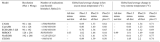
The HAPPI experimental protocol was inspired by the Climate of the 20th Century Plus Detection and Attribution (C20C+ D&A) project (Stone et al., 2018) and data from both sets of simulations are available at the same website (http://portal.nersc.gov/c20c/). However, only output from the MIROC5 model was submitted to both projects. In the HAPPI experimental protocol, the present-day forcings and boundary conditions are representative of the observed 2006–2015 state and are identical to that specified in the C20C+ D&A protocol over that period. HAPPI forcings for stabilized future scenarios preserve the observed 2006–2015 interannual variability (Stone et al., 2018; Mitchell et al., 2017) but include appropriate changes derived from CMIP5's RCP2.6 and RCP4.5 scenario simulations. Years for these simulations are nominally 2106–2115 as atmospheric trace gas concentrations are scaled from the RCP's protocol at 2095. Table 1 summarizes details of the model simulations used in this study. Note that the ensemble sizes are exceptionally large for a publicly available multi-model climate simulation dataset.

Table 1 Details of the HAPPI models used in this study. The number of realizations for each part of the numerical experiment is used separately in this study. For some individual years of the all-hist and nat-hist simulations, additional realizations may be available. The two rightmost columns show the globally averaged difference between selected combinations of the hot season temperature and the 20-year return value of the annual maximum 3-day average daily maximum surface air temperature (TX3x) over land. “Hot season” is defined as the maximum of June, July and August (JJA) and December, January and February (DJF) averages. Plus2.0 denotes the 2 ^∘C stabilization scenario and plus1.5 denotes the 1.5 ^∘C stabilization scenario. Note that CESM1 is not part of the HAPPI experiment but a fully coupled ocean-atmosphere climate model that has been run with emissions scenarios consistent with both targets. The CESM1 experiments are roughly comparable to the HAPPI experiment but not exactly the same forcing or reference period.

In this study, we examine the differences in changes in extreme temperatures from the HAPPI simulations. In a companion paper, we examined such changes between the actual and counterfactual (non-industrialized) simulations submitted to the C20C+ D&A project and this paper uses the same extreme value statistical methodologies (Wehner et al., 2018). The annual maximum of the daily maximum temperature is one of the 27 indices defined by the Expert Team on Climate Change Detection Indices (ETCCDI) and is a robust indicator of extremely hot weather (Zhang et al., 2011). Called “TXx” by the ETCCDI and derived from “tasmax”, the daily maximum near-surface air temperature in the CMIP5, this quantity is also known as “hot days” because it is the hottest daytime temperature of the year. As in our previous work on this topic (Tebaldi and Wehner, 2016; Sanderson et al., 2017; Wehner et al., 2018), we first calculate the running 3-day average of tasmax and compute its annual maximum, denoted hereafter as TX3x, and then estimate its 20-year return values by fitting stationary generalized extreme value (GEV) distributions. We have previously found that while long period return values of TX3x are slightly smaller than the values for the daily quantity, projected changes of the 3-day averages were considerably larger (Tebaldi and Wehner, 2016). For this study, where we are interested in the small differences between the 1.5 and 2.0 ^∘C stabilization levels, this point becomes particularly important.

In this paper, we do not assess the HAPPI models' relative skill at reproducing observed estimates of extreme temperatures. However, we note that this set of models form the atmospheric components of several of the CMIP5 fully coupled models. Sillman et al. (2013) examined the CMIP5 model's performance in simulating TXx and other ETCCDI measures. The coupled models corresponding to these five HAPPI models spanned a large range of TXx errors when compared to four different reanalyses. These model errors are presumably reduced when the ocean is specified to its observed state.

As in our C20C+ D&A analysis of anthropogenic extreme temperature changes, we estimate 20-year return values by fitting the GEV distribution by the methods of L-moments (Hosking and Wallis, 1997). Assumptions that the analyzed data are stationary and independent and identically distributed (i.i.d) are necessary for this approach to be valid and are reasonable for the HAPPI model output. A more detailed discussion of the rationale and limitations of these assumptions for the C20C+ D&A data is provided in Wehner et al. (2018) and the same arguments hold for the HAPPI data. Originally introduced by Zwiers and Kharin (1998) and Kharin and Zwiers (2000) to provide statistically rigorous projections of future extreme temperature and precipitation, such GEV analyses, both stationary and non-stationary, are now widespread throughout the literature including recent assessment reports of the International Panel on Climate Change (Seneviratne et al., 2012; Collins et al., 2013). The particulars of the details of the GEV analysis used in this study are described in the Supplement of Tebaldi and Wehner (2018).

By pooling the block maxima variable, TX3x, across both years and ensemble members, the extreme value time series are equivalent in length to the product of these two dimensions. As both the historical and stabilization periods are a decade, this results in extreme value sample sizes for the HAPPI models that are 10 times longer than the number of realizations in the 3rd column of Table 1, ranging from 500 (MIROC5) to 5000 (CAM4). These large sample sizes of the HAPPI models (Table 1) ensure that uncertainty due to the fitting of statistical distributions is negligible. The coupled model results (CESM1) are taken directly from Sanderson et al. (2017), which used periods of three decades to compensate for the smaller ensemble size.

3 Results

We limit this study to reporting changes in 20-year return values of extreme temperatures with the recognition that changes in longer period return values do not differ greatly. This is principally due to the bounded nature of the fitted GEV distributions and little difference in the width of these distributions over most land areas (Wehner et al., 2018). As changes in return periods for fixed thresholds are not as stable to the choice of threshold values, any results we might report would be of less general utility, so we defer such results to more targeted impact analyses. Figure 1 shows the changes over land in 20-year return values of the annual maximum of the 3-day average of daily maximum surface air temperatures (TX3x) between the 1.5 ^∘C stabilized scenario and the present-day simulations. Of the HAPPI models, MIROC5 exhibits the largest increases of the five HAPPI models, exceeding 0.75 ^∘C nearly everywhere and even 1.25 ^∘C over large regions. CAM4 and ECHAM6 exhibit the smallest changes but have hot spots in Asia. CanAM4, ECHAM6 and NorESM1 also show decreases or little increase over parts of the Amazon, but MIROC5 does not. The fitted GEV parameters and these return value changes are extremely robust to sample size uncertainty due to the large number of realizations in the HAPPI database (Table 1). Standard errors determined by a bootstrap calculation (Hoskins and Wallis, 1997) are very small. Results shown in Figs. 1–4 from the coupled ocean-atmosphere model CESM1 are shown for illustrative purposes only and are not directly comparable to the HAPPI models as the experimental protocols are necessarily different.

Figure 1 Change in 20-year return values (^∘C) between the 1.5 ^∘C and present-day HAPPI simulations of TX3x. (a) CAM4. (b) CanAM4. (c) ECHAM6. (d) MIROC5. (e) NorESM1. (f) CESM.

The annual maximum of the daily high temperature is most likely to occur in the summer over most of the world outside of the tropics. Figure 2 shows the difference between the 1.5 ^∘C stabilized scenario and the present-day simulations of the average surface air temperature in the hottest season, usually June, July and August (JJA) in the Northern Hemisphere and December, January and February (DJF) in the Southern Hemisphere. This much more spatially smooth average temperature change is quite different from the extreme temperature change in other ways as well. Global land average changes (shown in Table 1) indicate that hot season temperatures generally increase slightly more than extreme temperatures. However, there are significant regional differences between models, as shown below in Fig. 6. Furthermore, there are no regions of average temperature decreases. Average temperature increases are always greater than 0.25 ^∘C.

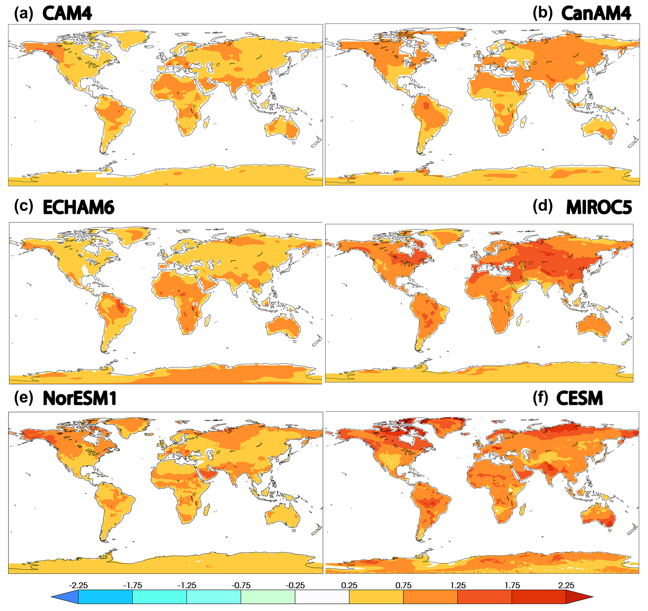
Figure 2 Differences in average hot season surface air temperature (^∘C) between the 1.5 ^∘C and present-day HAPPI simulations. (a) CAM4. (b) CanAM4. (c) ECHAM6. (d) MIROC5. (e) NorESM1. (f) CESM.

Figure 3 shows the changes over land in 20-year return values of the annual maximum of the 3-day average of daily maximum surface air temperatures between the 2.0 ^∘C stabilized scenario and the present-day simulations. As might be expected, extreme temperature increases are larger than in the 1.5 ^∘C stabilized scenario (Fig. 1). In this warmer scenario, most models produced no decreases in extreme temperature. Only ECHAM6 has a small decrease in the Amazon. For completeness, differences between the 2.0 ^∘C stabilized scenario and the present-day simulations of the average surface air temperature in the hottest season are shown in the Appendix. As in the cooler scenario, global averaged land extreme temperature differences are generally smaller than for the average hot season temperature differences (Table 1). MIROC5, discussed in more detail below, is an exception to this conclusion.

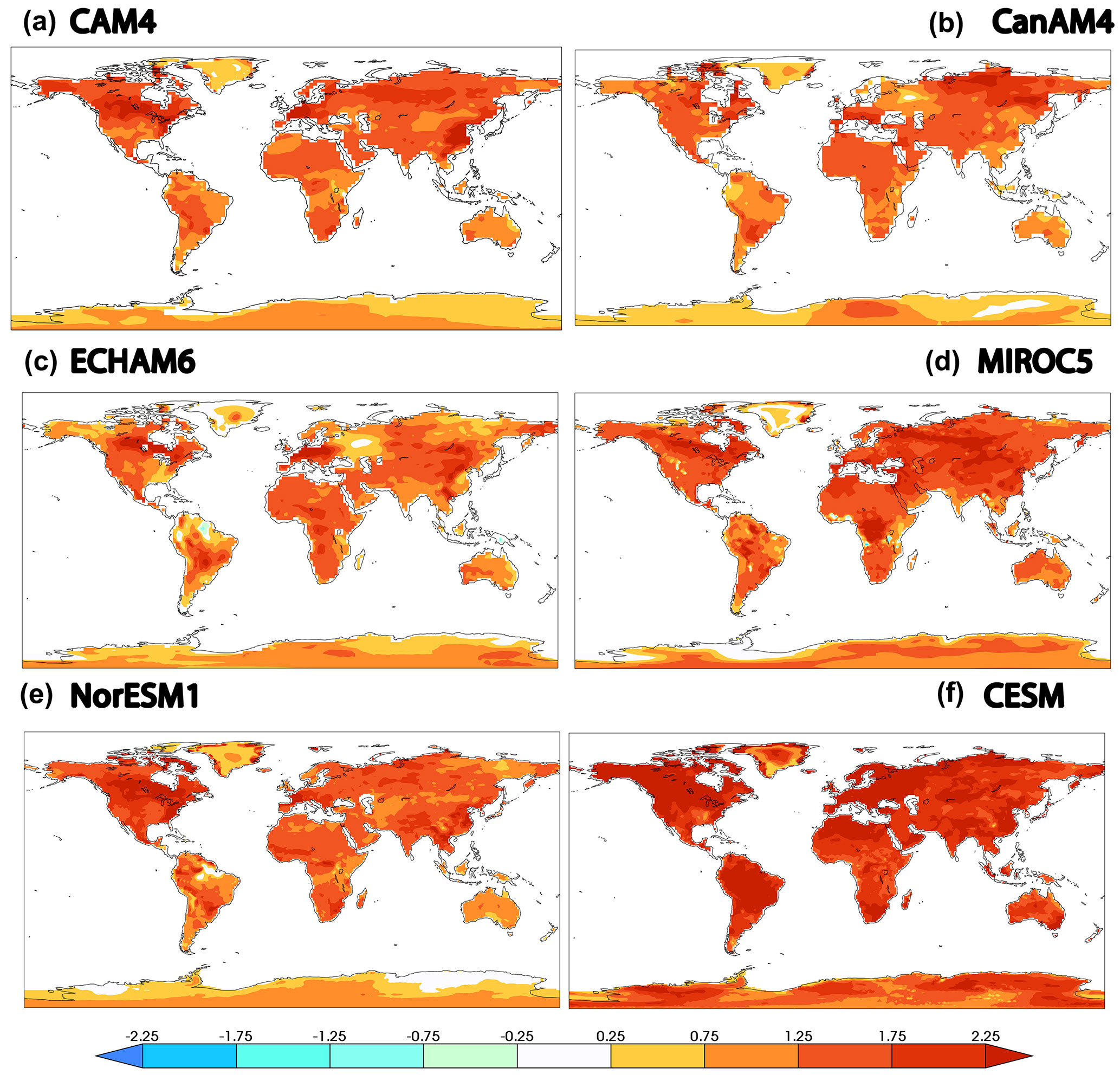
Figure 3 Change in 20-year return values (^∘C) between the 2.0 ^∘C and present-day HAPPI simulations of TX3x. (a) CAM4. (b) CanAM4. (c) ECHAM6. (d) MIROC5. (e) NorESM1. (f) CESM.

Differences between the extreme temperatures of the 2.0 and 1.5 ^∘C stabilized scenarios are shown in Fig. 4. Global land average differences in extreme 3-day hot temperatures range from about 0.5 to 0.75 ^∘C (Table 1).

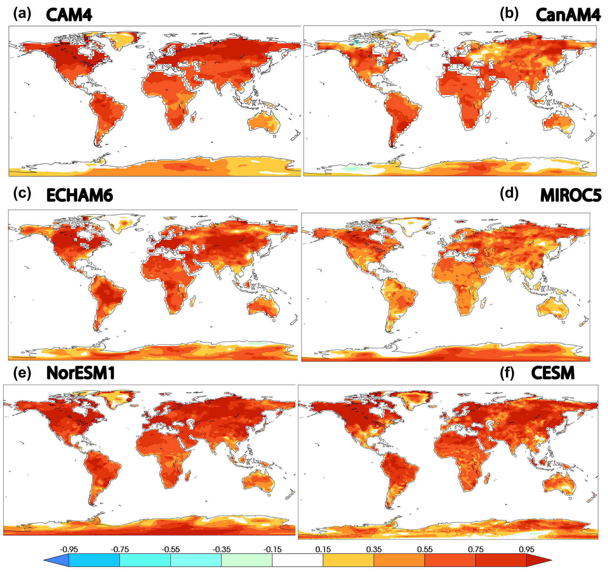
Figure 4 Differences in 20-year return values (^∘C) between the 2.0 and 1.5 ^∘C HAPPI simulations of TX3x. (a) CAM4. (b) CanAM4. (c) ECHAM6. (d) MIROC5. (e) NorESM1. (f) CESM. Note that the color scale covers a smaller range of temperature differences than for the previous figures.

Standard errors obtained from the method of Hoskins and Wallis (1997) are shown to be small in Fig. A3 of the Appendix. Generally, these error estimates are less than 0.15 ^∘C with the largest values towards the higher northern latitudes. Variability in CanAM4 is higher than the other HAPPI models but is generally less than 0.25 ^∘C. Standard error estimates in the CESM are of a similar magnitude but are not directly equivalent. Most of the changes in Figs. 1–4 are interpreted as at least at the likely level in the IPCC calibrated language (Mastrandrea et al., 2010).

At this time, only a single coupled model, the CESM, has been run under 1.5 and 2 ^∘C stabilization conditions. Fortunately, a moderately sized ensemble of those CESM simulations is available and analyzed in Sanderson et al. (2017) and shown in the lower-right panel of Figs. 1–4. The reference period from the “historical” run in Sanderson et al. (2017) was earlier than for the HAPPI all-hist simulation and partly explains the larger changes in the comparison between stabilization and current simulations shown in Figs. 1–3. Although the method to simulate stabilized climates is quite dissimilar between the HAPPI and the coupled model, differences between the 1.5 and 2.0 ^∘C stabilized CESM simulations of TX3x return values are quite similar to CAM4, ECHAM6 and NorESM1 with global averages over land of 0.7 ^∘C or larger.

The MIROC5 is the only model for which results were submitted to the C20C+ D&A project. In Wehner et al. (2018), we find that anthropogenic aerosol forcing can play a critical role in heat wave attribution statements. The MIROC5 experiments were run with a fully prognostic sulfate, black carbon and organic carbon aerosol package forced by prescribed aerosol emissions. In such experiments, aerosol concentrations can interact with the immediate meteorology, leading in some regions to cooling, especially in events characterized by persistent and stagnant air masses. This is indeed the case for the MIROC5 all-hist simulations compared to the C20C+ D&A counterfactual simulations (nat-hist) of a world without anthropogenic changes to the composition of the atmosphere. All-hist minus nat-hist extreme temperatures from MIROC5 are replotted from Wehner et al. (2018) in the top panel of Fig. 5 with a wider color scale to permit additional comparison to the warmer stabilization scenarios. Decreases in extreme temperatures are found in East Asia, the Congo and Eastern Europe that are attributable to sulfate and organic carbon aerosol concentration differences for this model. In the MIROC5 stabilization runs, sulfate and organic carbon aerosol emissions are reduced according to the protocols of the RCP2.6 scenario. These reductions allow the greenhouse gas contribution to temperature changes to dominate, leading to increases in these regions when comparing the stabilization experiments to either the all-hist or nat-hist MIROC5 experiments (Figs. 1, 3 and 5). In fact, the cooling in these regions in the MIROC5 all-hist experiment results in localized hot spots when compared to the stabilization experiments (Figs. 1 and 3). This is especially evident over the Congo in these figures.

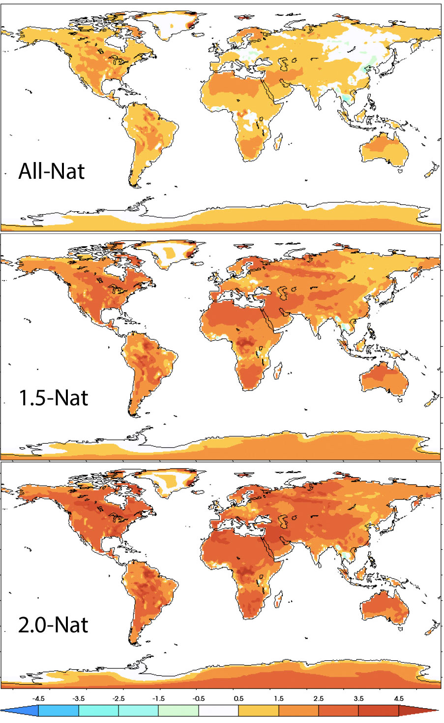
Figure 5 Change in 20 year return values (^∘C) of TX3x between the C20C+ D&A counterfactual simulation of a non-industrial world and the present-day, 1.5 ^∘C, 2.0 ^∘C HAPPI simulations for the MIROC5 model. Note that the color scale covers a larger range of temperature differences than for the previous figures.

4 Discussion

The HAPPI coordinated climate modeling experiments demonstrate that there are indeed benefits in the form of reduced heat wave intensities associated with lower stabilization targets. The large number of realizations permits estimation of these reductions in heat wave magnitude to a high precision for each of the four participating models. For two of the models (CanAM4 and MIROC5), heat wave differences between the 1.5 and 2 ^∘C stabilization targets called for in the Paris Agreement are close to 0.5 ^∘C over large portions of the land mass. The other 3 models showed reductions of approximately 0.75 ^∘C over large regions of the land mass.

The HAPPI experimental protocol was designed to explore roughly equal increments of global warming with experiments of the present day, approximately 1 ^∘C above preindustrial temperatures, compared to 1.5 and 2 ^∘C above that reference value. However, comparing the changes between the 1.5 ^∘C stabilization and present day to the changes between the 2.0 and 1.5 ^∘C stabilizations reveals profound differences across models in the pattern of warming, both in mean and extreme temperatures. This is traceable in part to the unconstrained nature of the aerosol forcings. Models vary in their response to aerosol forcing, especially in the so-called “indirect” effect involving feedbacks with cloud nucleation processes. However, more relevant to temperature extremes is the fact that some models prescribed atmospheric aerosol concentrations while others prescribed aerosols emissions. In the former case, aerosol concentrations are slowly varying and independent of the local meteorology. In the latter case, aerosol concentrations interact with the meteorology and can be considerably larger than their climatological averages during the stagnant conditions often associated with certain types of heat waves. Higher aerosol concentrations lead to greater atmospheric reflectivity reducing temperatures during such heat waves. In the RCP2.6 scenario, emissions of sulfate aerosols are significantly reduced compared to the present day. Hence, the type of aerosol treatment can affect magnitudes of the changes in simulated TX3x return values. Relative to the non-industrial MIROC5 simulations, present-day heat waves are suppressed in East Asia and other areas where sulfate aerosol emissions are currently high. As aerosol emissions in the stabilization scenarios are reduced from present-day levels, changes in heat waves are larger in these regions because of this suppression. This is a possible explanation of some of the differences between simulated TX3x return values in the stabilized scenario compared to the present day. On the other hand, aerosol forcing in the two stabilization scenarios are the same, leading to a more controlled comparison of the effects of increased greenhouse gases. As a result, the differences between stabilization scenarios in extreme temperature changes shown in figure 4 are less spatially heterogeneous and more similar between models than changes relative to the present day (Figs. 1 and 3).

This relative uniformity in Fig. 4 suggests that pattern scaling of extreme temperature changes in models in the CMIP5 forced by the RCP2.6 forcings to the 1.5 ^∘C stabilization target may be an appropriate method to accurately estimate changes in extreme temperatures. However, relating changes in average hot season temperatures to changes in long period return values of TX3x is difficult in the low-warming stabilization scenarios considered here. Figure 6 shows the difference between changes in 20-year return values of TX3x and changes in hot season average temperatures for the 2.0 ^∘C stabilization scenario relative to the historical period. There is no clear relationship across models between changes in the middle of the temperature distribution to changes in the tail. For instance, CanAM4 exhibits smaller changes in the TX3x return values than in the hot season average. The couple model, CESM, exhibits the opposite behavior. The other four HAPPI models are mixed with some regions exhibiting greater changes in extreme temperatures but other regions exhibiting lesser changes. The exaggerated effects on extreme temperatures of aerosol forcing changes would tend to lead to larger changes in extreme temperature than for hot season temperatures in the prescribed aerosol emission models since RCP2.6 reduces aerosol forcing. Hence, this mechanism may be partly responsible for the heterogeneities in East Asia and the Congo of Fig. 6 but is not likely a factor for the heterogeneities in North America and Europe.

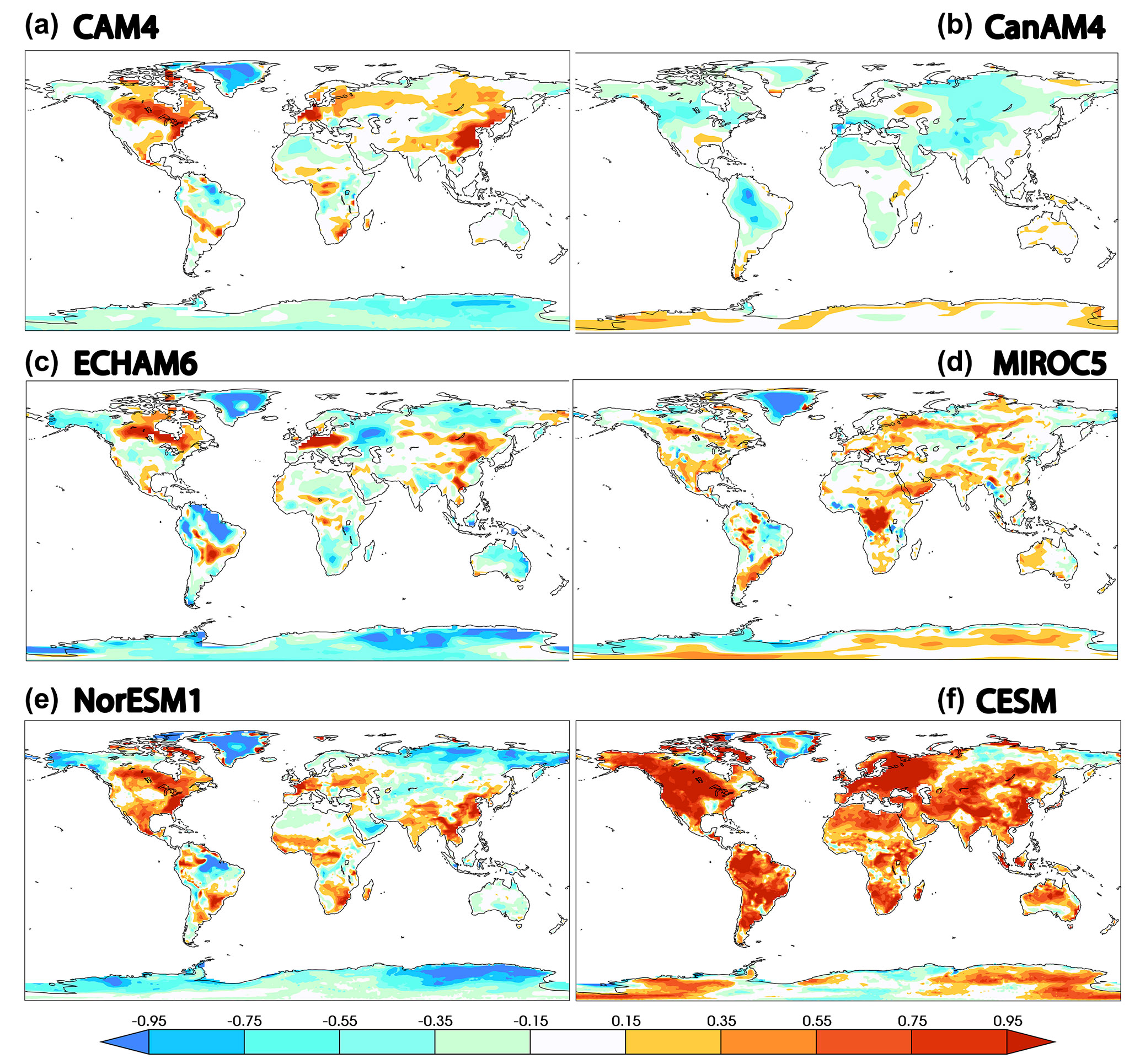
Figure 6 Differences between changes in 20-year return values of TX3x and changes in hot season average temperatures (^∘C) in the 2.0 ^∘C HAPPI simulations. (a) CAM4. (b) CanAM4. (c) ECHAM6. (d) MIROC5. (e) NorESM1. (f) CESM.

Land surface feedbacks offer another mechanism for different patterns of hot season and extreme temperature changes. Evaporative cooling fueled by surface soil moisture can locally reduce surface air temperatures (Seneviratne et al., 2010). However, as the supply of surface soil moisture is limited, such temperature reductions by evaporative cooling are also limited (Vogel et al., 2017). Hence during extended periods without rain, dry conditions can enhance extreme high temperatures. If this mechanism were important, one would expect changes in extreme temperatures to be larger than average hot season temperature in regions with moderate amounts of hot season rainfall.

Both the aerosol forcing and land surface feedback mechanisms would lead to locally larger changes in extreme temperature compared to hot season temperatures. We note that both mechanisms are diminished as greenhouse gas forcing increases past those imposed by the HAPPI protocols. A physical mechanism for the smaller extreme temperature changes in Fig. 6 is not readily apparent although changes in large scale circulation are certainly a possibility (Koster et al., 2014). Also, Fischer and Schär (2009) found a lengthening of the summer season in parts of Europe that could also raise the average seasonal temperature more than short duration extremes. In any event, we discount the possibility that these regions of smaller extreme temperature changes are a result of statistical uncertainties due to the large number of HAPPI realizations in each ensemble.

The lack of a clear relationship in these models between hot season and extreme temperature changes would seem to contradict the results of Seneviratne et al. (2016) who found an approximately linear relationship between average regional changes in TXx and changes in annual global mean temperature with slopes greater than unity (i.e., extremes change more than the global mean). In general, we feel that comparison of changes in very hot days to hot season average temperature changes is more instructive than comparison to annual mean temperature changes in order to more isolate relevant physical mechanisms of changes. For instance, changes in albedo due to snowmelt may cause larger winter temperature changes than temperature changes in other seasons. However, the methods used to draw conclusions from our study and Seneviratne et al. (2016) are too dissimilar to reveal contradiction. Figure 6 shows a relationship between local temperatures for individual models, while the results in Seneviratne et al. (2016) are a multi-model re-expression of transient extreme temperature changes in terms of global mean temperature instead of either time or greenhouse gas forcing.

5 Conclusions

Climate model experiments with identically prescribed SST and sea ice concentration such as the ones presented here have a computational advantage that permits a large number of realizations enabling precise statistical description of extreme temperatures. However, the limited number of models participating in the HAPPI experiment does not sample the model structural uncertainty as fully as the CMIP5 database of coupled models and the spread in results presented here should not be interpreted as a complete representation of the uncertainty in the extreme temperature change stabilized scenarios. Nonetheless, although there is some amplification of extreme temperature differences relative to average hot season temperature differences between the 1.5 and 2.0 ^∘C stabilization targets, this amplification does not appear to be dramatic.

Appendix A

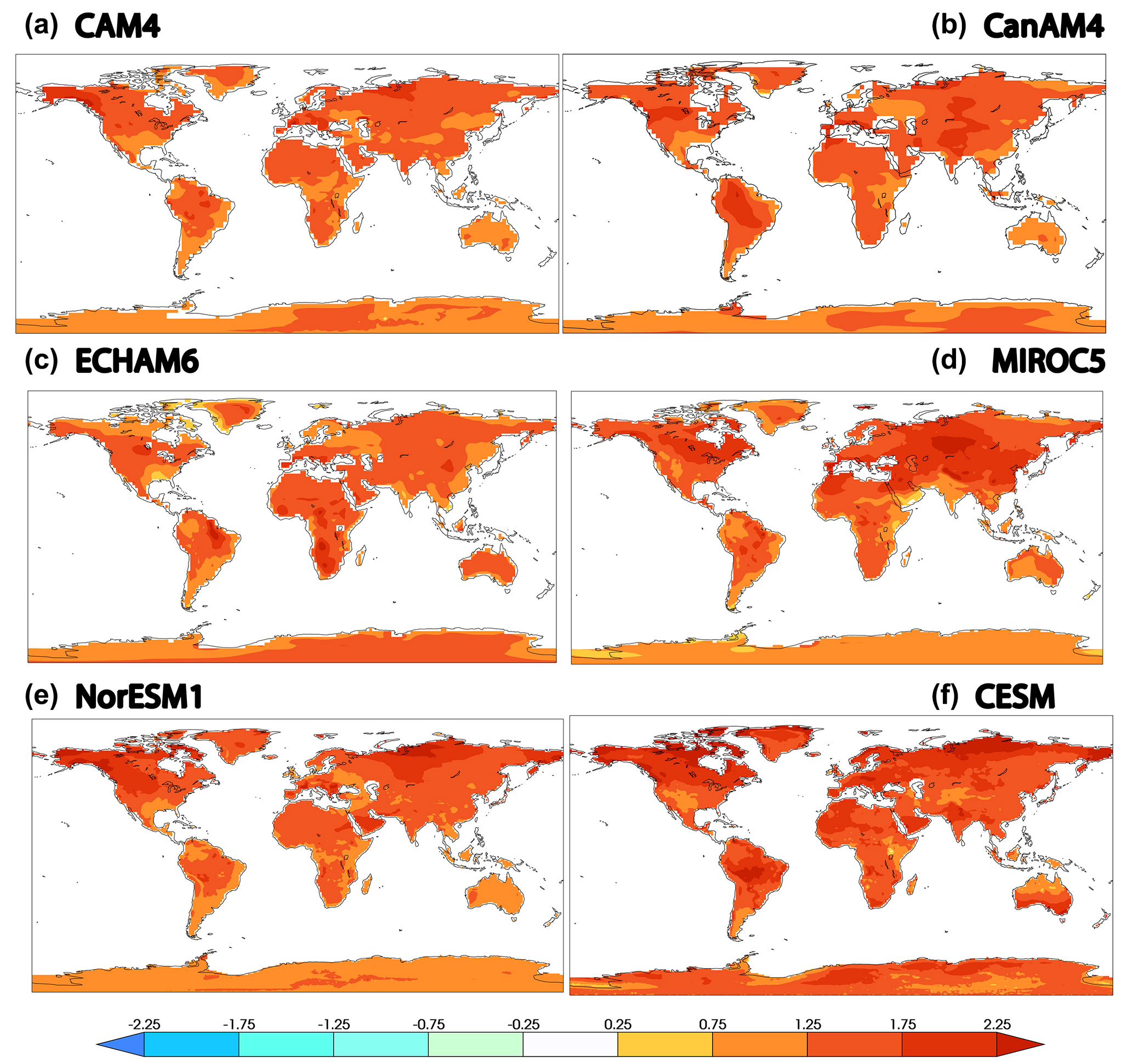
Figure A1 Differences in average hot season surface air temperature (^∘C) between the 2.0 ^∘C and present-day HAPPI simulations. (a) CAM4. (b) CanAM4. (c) ECHAM6. (d) MIROC5. (e) NorESM1. (f) CESM.

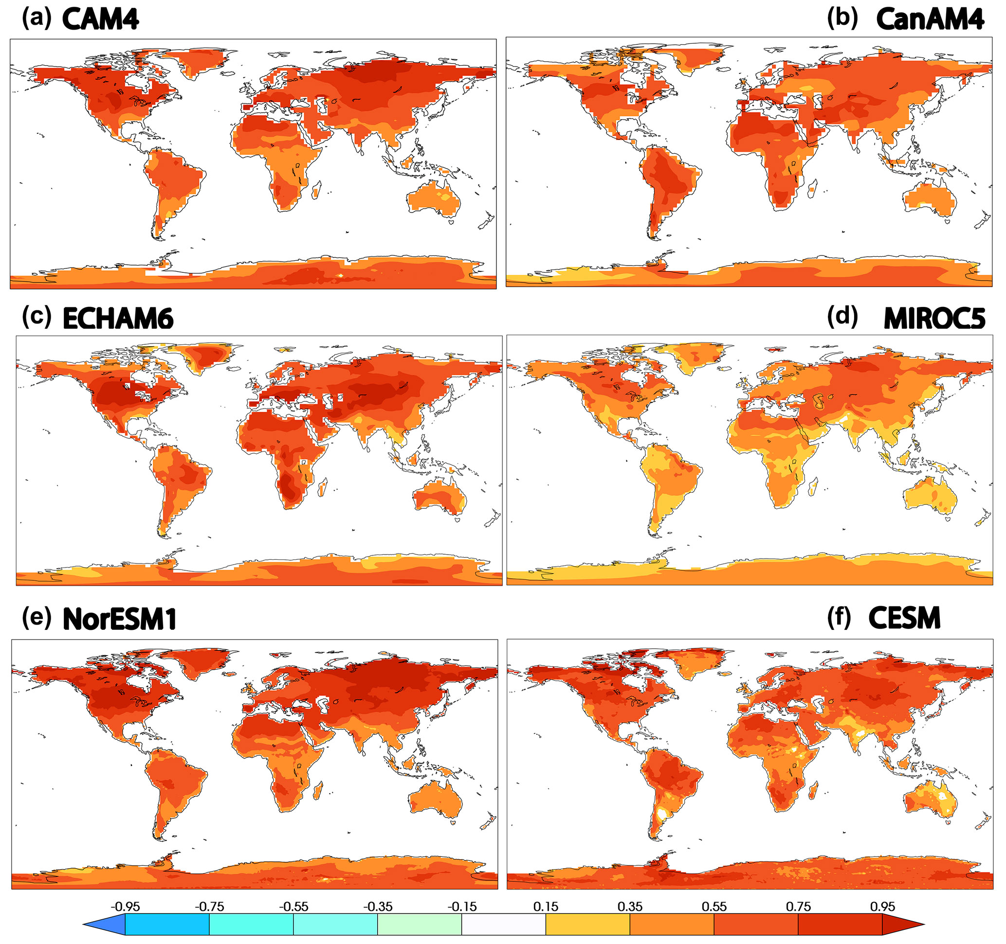
Figure A2 Differences in average hot season surface air temperature (^∘C) between the 2.0 ^∘C and 1.5 ^∘C HAPPI simulations. (a) CAM4. (b) CanAM4. (c) ECHAM6. (d) MIROC5. (e) NorESM1. (f) CESM.

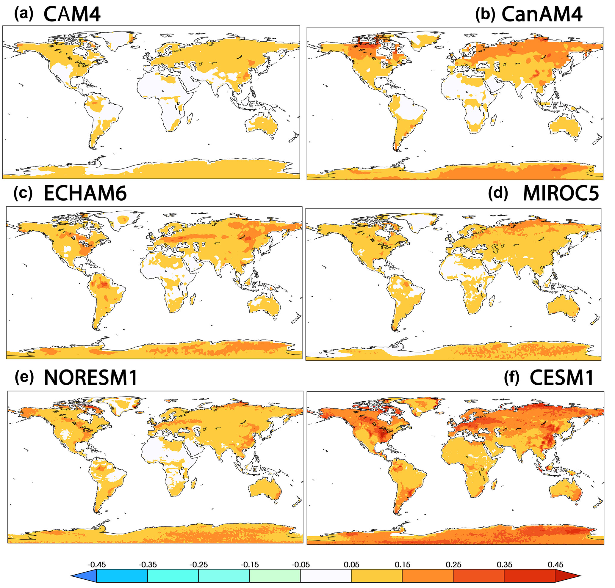
Figure A3 Standard error estimates of 20-year return values of TX3x (^∘C) in the 1.5 or 2.0 ^∘C HAPPI simulations. (a) CAM4. (b) CanAM4. (c) ECHAM6. (d) MIROC5. (e) NorESM1. (f) CESM.