A multivariate analysis of atmospheric drivers for Western European heatwaves

Understanding the dynamics of heatwaves is critical for accurate climate risk assessment. Traditional definitions, based solely on surface temperature thresholds, can detect heatwaves but cannot be used to analyze the complex, multivariate nature that causes them. We apply a spatiotemporal Variational Autoencoder (VAE) to ERA5 reanalysis data to identify compact representations of multivariate, year-round heatwave patterns over Western Europe. Focusing on key atmospheric variables (e.g. circulation, humidity, temperature, geopotential height, cloud cover, stream function, and radiation), we extract 11 d heatwave samples from ERA5 reanalysis data over the North Atlantic, centered on near-surface temperature extremes in Western Europe. The VAE was trained on heatwave samples from 1941 to 1990 and evaluated using samples from 2001 to 2022, effectively clustering heatwave events by season and identifying known dynamical regimes, such as summer blocking highs and winter omega blocks. The VAE model captures the interplay and temporal evolution between different atmospheric variables in their contributions to heatwaves over Western Europe. Notably, the VAE identifies distinct atmospheric circulation patterns that align with seasonal dynamics even when applied to detrended and deseasonalized data. When analyzing non-detrended data, recent summer heatwaves occupy a distinct region in the latent space, consistent with the strong warming-driven intensification of these events. However, analyses of detrended data reveal significant structural shifts in atmospheric configurations across all seasons, indicating that the VAE captures changes in the multivariate structure of heatwave-related variables beyond simple mean warming. Composite anomaly maps further show coherent pre-onset patterns across variables. These results demonstrate the utility of VAEs for extracting physically meaningful, multivariate representations of heatwave dynamics from reanalysis data, highlighting changes in their atmospheric drivers over recent decades.

1 Introduction

Extreme events and heatwaves pose a significant threat to both the environment and human health (López-Bueno et al., 2021; Mora et al., 2017a). Extreme events refer to rare and intense meteorological phenomena, whereas heatwaves are characterized by exceptionally high temperatures that persist over several days. Since the effects of climate change intensify with the increased amount of human-induced greenhouse gases in the atmosphere (Lynas et al., 2021), the frequency and intensity of hot (cold) extremes increase (decrease) globally (IPCC, 2021). On average, the intensity of hot extremes increases approximately linearly with global warming, while the frequency of rare hot extremes increases more rapidly (IPCC, 2021; Li et al., 2021; Fischer and Knutti, 2014; Kharin et al., 2018; Fischer et al., 2021; Skinner et al., 2025). These trends are projected to continue even at the lowest projected global warming scenario (IPCC, 2021).

Currently, 30 % of the global population is exposed to deadly climatic conditions, which are projected to increase up to 75 % under the current greenhouse gas emissions scenarios (Mora et al., 2017a, b; King and Harrington, 2018). The growing severity of extreme events also impacts the environment, infrastructure, and economy (Yuan et al., 2024; Dosio et al., 2018; IPCC, 2021). Recent heatwaves in Europe (2003, 2010, 2015, and 2018) caused damages that amounted to 0.3 %–0.5 % of European gross domestic product (GDP) (García-León et al., 2021). Globally, the annual cost of extreme weather events is estimated at USD 143 billion (Newman and Noy, 2023). Looking ahead, global cumulative GDP losses could reach 16 %–22 % by the end of the century if the current 3 °C warming trajectory continues (Burke et al., 2015; Newell et al., 2021; Kotz et al., 2024; World Economic Forum, 2024). Therefore, identifying and characterizing heatwaves is crucial to effectively mitigating and adapting to their impacts. Since extreme temperature events, including heatwaves, are by definition rare occurrences at the tails of temperature distributions (McPhillips et al., 2018), percentile and block maxima methods have been widely used for their detection (Zhang et al., 2011; Huang et al., 2016; Alaya et al., 2020; Li et al., 2021; IPCC, 2021). Russo and Domeisen (2023) demonstrated that historically unprecedented extreme heatwaves have increased 10-fold in recent years, using cumulative indices for their identification rather than indices relying on temporal averages, as cumulative indices are more reliable for comparing events with different durations. Brunner and Voigt (2024) found that seasonal running windows commonly used to define extreme thresholds can introduce systematic biases and underestimate the frequency of extreme events. However, the definition of an extreme depends on the application, and there is no standard definition for heatwaves (Barriopedro et al., 2023; Boni et al., 2023). Many existing indices rely solely on temperature, which allows detection but provides only limited information to capture the full complexity of these events (Perkins, 2015; McPhillips et al., 2018; Barriopedro et al., 2023). The complex nature of heatwaves, however, requires more sophisticated analysis methods. Multiple atmospheric processes and local drivers play an essential role in the occurrence of heatwaves, and a multidimensional approach considering the tails of high-dimensional, multivariate probability distributions, whose shape and structure are themselves changing due to non-stationary climate dynamics, is required for defining and studying heatwaves (Sardeshmukh et al., 2015; Domeisen et al., 2022; Barriopedro et al., 2023; Camps-Valls et al., 2025).

Machine learning (ML) and deep learning (DL) methods are frequently employed in climate science, as they can uncover complex relationships in multivariate and high-dimensional climate datasets (Reichstein et al., 2019; Zhu et al., 2023; Salcedo-Sanz et al., 2023; Camps-Valls et al., 2025). For instance, Ronco et al. (2023) employed explainable machine learning models, including random forests and gradient boosting, to predict human displacement induced by floods, storms, and landslides from global observational data. Machine learning methods help discover physical processes from data and improve numerical simulations (Heuer et al., 2024; Debeire et al., 2025). Unsupervised approaches such as autoencoders and clustering can extract dynamical regimes from high-dimensional climate fields, advancing physical understanding beyond traditional linear methods (Lai et al., 2025; Behrens et al., 2022). ML and DL techniques rely on high-quality and reliable labeled data (Camps-Valls et al., 2025). However, a significant limitation for extreme events and heatwaves is precisely the lack of high-quality and labeled datasets (Prabhat et al., 2021; Lacombe et al., 2023). One potential solution is to use unsupervised learning methods where the model learns patterns from data autonomously. Unsupervised learning methods help identify complex data patterns without relying on predefined labels or thresholds (Kingma and Welling, 2019). In Paçal et al. (2023), the Gaussian Mixture Model (GMM), an unsupervised learning approach that models data as a combination of multiple Gaussian distributions, was applied to characterize extreme temperature events. By representing daily maximum temperatures as a bimodal rather than a traditional unimodal distribution, the study found that extreme temperature events will become significantly more frequent under future global warming levels and revealed regional differences not captured by conventional methods. Another example of an unsupervised learning method is the Variational Autoencoder (VAE), which is composed of an encoder that reduces the dimensionality of the input data to a latent space and a decoder that reconstructs the input data from that latent space (Kingma and Welling, 2019). Recent advances in artificial intelligence for climate extremes have highlighted the importance of unsupervised learning models like GMMs and VAEs for both detecting anomalies and uncovering the mechanisms behind rare and compound events, especially when labeled data are scarce or absent (Materia et al., 2024).

VAEs are primarily developed as generative models, capable of learning complex data distributions and generating realistic synthetic samples (Kingma and Welling, 2019). Beyond generative tasks, VAEs have also been widely applied in anomaly detection across various domains, including network security, risk management, health monitoring, and computer vision (Pang et al., 2021; Nassif et al., 2021; Albuquerque Filho et al., 2022). Among other applications, autoencoders and VAEs have been applied to learn spatiotemporal regularities from video data (Hasan et al., 2016; Fan et al., 2020). VAEs and clustering methods such as GMMs have been used to identify regimes in the latent space and analyze their dynamical behavior in climate science (Lindhe et al., 2021; Happé et al., 2024; Paçal et al., 2023). Spuler et al. (2024) introduced the RMM-VAE, a probabilistic machine learning method that combines variational autoencoders with clustering to identify circulation regimes targeted to local impact variables. Happé et al. (2024) applied a 3D variational autoencoder to heatwave events from the KNMI-LENTIS dataset over western Europe, showing that the latent space captures physically interpretable circulation regimes and that heatwaves are best represented in a probabilistic framework.

Building on these previous applications, our study extends Happé et al. (2024) to a multivariate and year-round analysis of European heatwaves using reanalysis data. This study aims to understand how heatwaves develop, what contributes to their evolution, and how recent heatwaves are represented relative to those from the historical baseline. In contrast to Happé et al. (2024), who focused on heatwave samples extracted from the KNMI-LENTIS dataset over Western Europe, we (i) include nine atmospheric variables from the ERA5 reanalysis dataset to assess their contribution to heatwave evolution, (ii) analyze spatiotemporal samples over a larger window (±5 d around the onset, i.e. 11 d in total) to characterize build-up and decay processes better, (iii) train on 11 d multivariate ERA5 heatwave samples that cover the full year with standardized anomalies, and (iv) assess generalization with an explicit historical-to-recent evaluation. To this end, we first train a spatiotemporal VAE on multivariate reanalysis heatwave samples from the historical period of 1941–1990. Then, we cluster and analyze the latent space representation of recent heatwaves (2001–2022) in Western Europe. Section 2 describes the data and methodology followed in this research. Section 3 provides the results for the heatwave cluster analysis. Finally, the main results are summarized and discussed in Sect. 4.

2 Data and Methods

2.1 Data Sources and Preprocessing

We used the ERA5 reanalysis dataset (Hersbach et al., 2017; Soci et al., 2024) to detect and understand heatwave dynamics. We focused only on atmospheric variables, as shown in Table 1, including those used in Happé et al. (2024) as well as additional variables relevant to heatwave dynamics identified in previous studies, such as geopotential height at 500 hPa (z₅₀₀) as it captures mid-tropospheric circulation patterns and has been shown to better reproduce temperature anomalies associated with European heatwaves than sea-level pressure (Jézéquel et al., 2018; Domeisen et al., 2022; Rousi et al., 2022; Barriopedro et al., 2023; Kim and Seo, 2023; Tian et al., 2024). All data was accessed via the German Climate Computing Center (DKRZ) data catalog (Hersbach et al., 2017). We aggregated hourly data in GRIB (General Regularly-distributed Information in Binary form) format for each variable into daily values using variable-specific temporal operators, such as daily maxima for temperature and daily means for pressure, as shown in Table 1. The resulting dataset comprises daily observations from 1940 to 2022 for the North Atlantic region, spanning from 75° W to 60° E and from 30 to 75° N on a 0.7° grid, as shown in Fig. 1. ERA5 data were regridded from its native 0.25° resolution to 0.7° to ensure direct comparability with Happé et al. (2024), which uses this resolution as the native grid of the EC-Earth3 model. Furthermore, this coarser resolution also reduces the very high dimensionality of the multivariate input while retaining the large-scale circulation patterns. Although ERA5's native resolution is finer, the reconstruction performed by the variational autoencoder emphasizes large-scale circulation patterns while smoothing out small-scale variability. Retaining the native 0.25° grid would therefore not provide additional benefit while substantially increasing computational cost. Since ERA5 data are provided in hourly resolution, we first applied the temporal aggregation operators listed in Table 1 to convert the hourly ERA5 fields to daily values. From these daily fields, we then computed the 1941–1980 climatological mean and standard deviation using a 15 d moving window centered on each calendar day, which we used to standardize the variables and remove seasonal variability. The 15 d climatological window is a common choice for smoothing day-to-day noise while preserving seasonal variations. This approach is consistent with other studies on extreme-event detection (Sulikowska and Wypych, 2020). We used this period to calculate the climatology, as it precedes the stronger warming trends after 1980 in Europe (Elguindi et al., 2013; Reid et al., 2016). The standardized daily anomalies were then used for all subsequent analyses.

Table 1 Overview of the atmospheric variables used for heatwave characterization in this study. The temporal operator refers to the daily aggregation method applied to each variable during preprocessing, converting the hourly frequency to a daily frequency. Heatwave samples for training and analysis, comprising all nine variables (multivariate), are extracted from the broader North Atlantic region, centered temporally around the onset dates. (^⋆) 2 m temperature (t2m) is used to identify heatwave onset dates specifically from the Western Europe subregion. Regions are shown in Fig. 1.

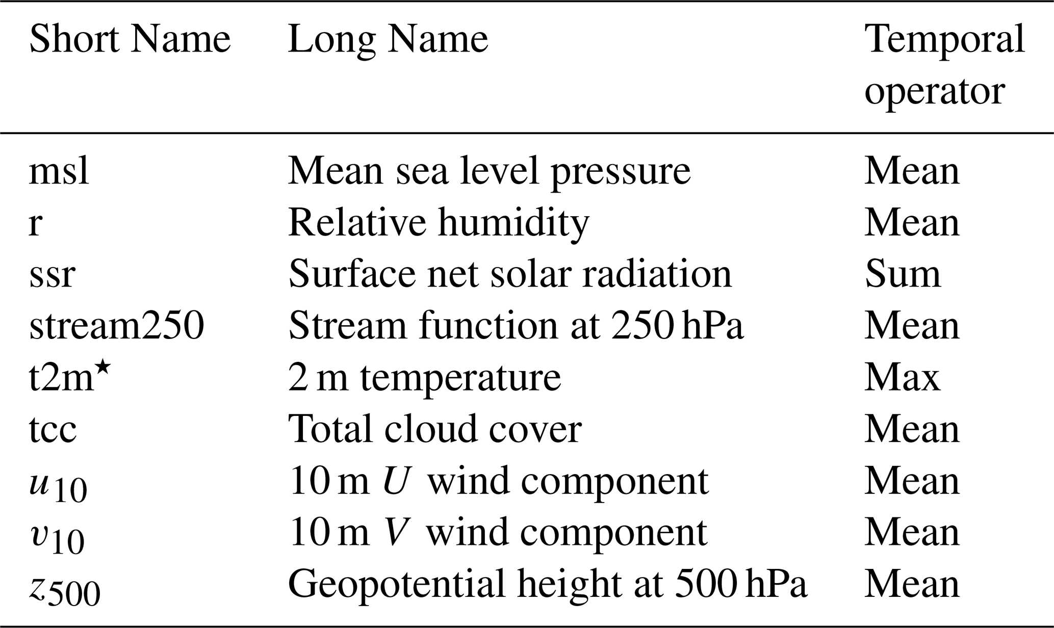
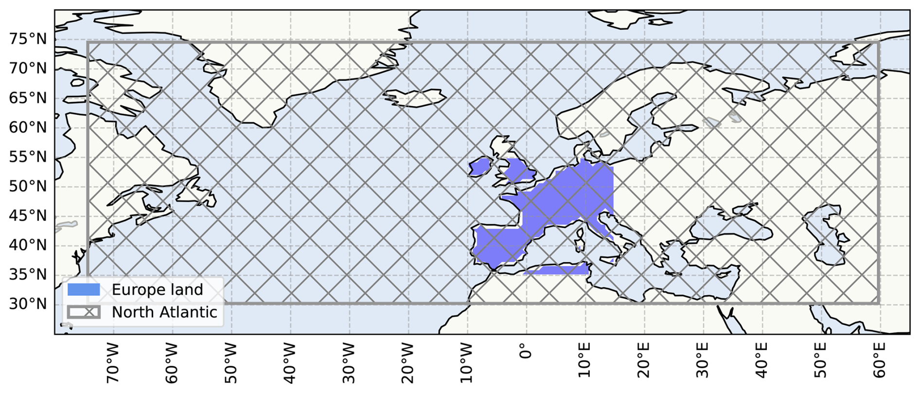
Figure 1 Geographical domains used to identify heatwave onset dates and train the VAE model. The shaded blue area represents the Western Europe land grid cells used to identify heatwave onset dates based on hot grid points derived from ERA5 temperature fields. These onset dates are then used to extract 11 d heatwave samples, centered on the onset dates, from the broader North Atlantic region (indicated by the hatched gray box), covering the nine variables (multivariate) listed in Table 1. These multivariate heatwave samples are used for training and analysis.

2.2 Heatwave Identification

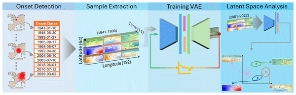
We followed the methodology proposed by Happé et al. (2024) to identify heatwave onset dates over Western Europe and extract heatwaves from the extended North Atlantic region. The identification process consists of three main steps: (1) threshold-based detection of anomalies at the grid-point level, (2) clustering of spatially and temporally contiguous anomalous grid cells, and (3) extraction of multivariate spatiotemporal samples suitable for model training. The overall workflow for heatwave onset detection and sample extraction is illustrated in Fig. 2.

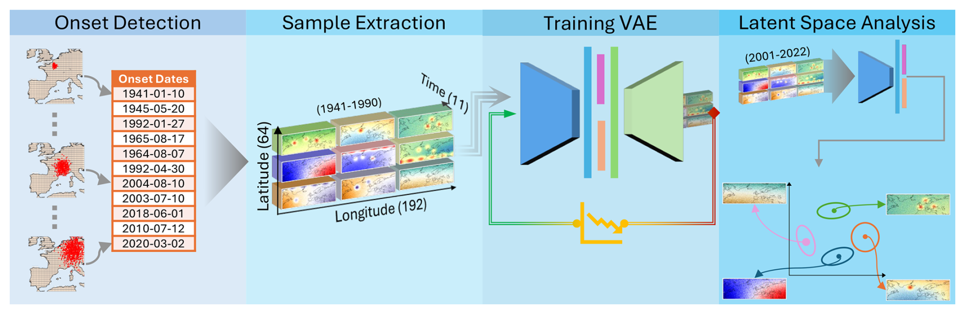
Figure 2 Workflow illustration of the heatwave onset detection and sample extraction process. Detected onset dates over Western Europe are used to extract 11 d multivariate heatwave samples from the North Atlantic region, centered on the onset of each event. Samples from 1941–1990 are used to train a Variational Autoencoder (VAE) that learns compact representations of the spatiotemporal structure of heatwaves. Subsequently, samples from 2001 to 2022 are encoded into the latent space to analyze the evolution and dynamics of recent heatwave events.

The first step is to detect anomalies at the level of individual grid cells. We focused only on land grid cells in the Western Europe subregion, extending from 10° W to 55° E and from 35 to 55° N (see the blue shaded area in Fig. 1). Then, we used daily maximum 2 m temperature data from the ERA5 reanalysis dataset. For each grid cell, we calculated the 90th percentile threshold for each calendar day using a multiyear 15 d moving window centered on that day, based on the historical baseline period from 1941 to 1980. We identified anomalies each day by comparing the temperature to the corresponding threshold. This approach captured relative temperature anomalies while accounting for seasonality and regional climate norms. The result was a binary mask indicating whether or not a grid cell experienced a day of anomalous heat. A value of 1 for a grid cell marks exceedance of the local threshold, while 0 represents climatologically typical conditions. Subsequently, during the second step, we applied the Generalized Density-Based Spatial Clustering of Applications with Noise (GDBSCAN) algorithm to detect heatwave events (Sander et al., 1998), using a minimum cluster size of 21 cells across space and time, as suggested by Happé et al. (2024). This procedure identified 2565 unique heatwave onset dates between 1941–2022 from land grid cells over Western Europe, as shown in Fig. 1.

Finally, the last step involves extracting heatwave samples using these onset dates, with 11 d windows centered on each onset. The 11 d window encompasses the five days preceding the onset, the onset day itself, and the subsequent five days, similar to Rouges et al. (2023). We focused on nine different atmospheric variables (multivariate), as listed in Table 1. In the first step, we only used land grid cells over Western Europe to define heatwave onset dates. However, the heatwave samples used for training the model and for analyses cover a broader spatial domain, namely the extended North Atlantic region, to capture large-scale atmospheric conditions, as shown by the hatched gray box in Fig. 1. This framing (spatiotemporal) captures both the build-up and evolution of heatwave conditions, enabling the VAE model to learn characteristic patterns associated with the heatwaves.

Compared to Happé et al. (2024), our setup differs in several ways. We focused on the ERA5 reanalysis dataset to extract heatwave samples, rather than the KNMI-LENTIS. Furthermore, we extracted heatwave samples across the year, avoiding a fixed definition of summer. This makes our approach more general and less dependent on a definition of “summer” (Wang et al., 2021). Additionally, the data are standardized, allowing us to analyze both summer heatwaves and anomalous heat during colder months, such as warm spells or winter heatwaves. This approach, in turn, allows for more heatwave samples from the ERA5 reanalysis dataset to be used for training the VAE model. An additional difference between our approach and the method applied in Happé et al. (2024) is that we used additional atmospheric variables to investigate their impact on heatwave occurrence and to analyze large-scale atmospheric patterns. We also incorporated timesteps before the onset of heatwaves (Rouges et al., 2023), allowing us to identify atmospheric patterns that build up to and persist during heatwave progression.

2.3 Variational Autoencoder

The Variational Autoencoder (VAE) is an unsupervised machine learning method that uses neural networks to generate a latent-space representation of the input data, enabling the reconstruction of the original input data (Kingma and Welling, 2019). VAEs have been widely and successfully used in anomaly detection, image recognition, and generative modeling (Pang et al., 2021). VAEs consist of an encoder network and a decoder network. The encoder network takes an input, x, such as an image, and compresses it into a latent-space representation. This latent space is represented as a probability distribution, typically a Gaussian. The decoder then takes the representation from the latent space and reconstructs the input, $\widehat{x}$. The main goal of VAE is to approximate the reconstructed output as closely as possible to the original input by minimizing the reconstruction loss between the output and input. A VAE, therefore, summarizes complex, high-dimensional data into a low-dimensional embedding. This low-dimensional latent space compresses the input data, enabling the discovery of hidden patterns. It can be further analyzed using visualization techniques and clustering algorithms to identify patterns and regimes in the data (Happé et al., 2024; Lindhe et al., 2021). The reconstruction produced by the VAE can be interpreted as a learned climatological baseline or “normal state,” against which deviations can be studied. We focused on using latent space to understand the atmospheric patterns underlying different heatwave types. Similar latent space approaches have been successfully applied in climate research (Behrens et al., 2022; Oliveira et al., 2022; Shamekh et al., 2023; Mooers et al., 2023; Camps-Valls et al., 2025).

We considered a 3D convolutional neural network architecture for our VAE model to learn multivariate spatiotemporal representations of heatwaves in an unsupervised manner (see Table A1 in the Appendix for the description of the VAE architecture and more details on the training process). We also experimented with hybrid architectures combining 2D convolutional encoder (decoder) layers to capture spatial features, followed (preceded) by LSTM (Long Short-Term Memory) layers to capture temporal information. However, these configurations produced unstable or less coherent reconstructions, likely because the LSTM struggled to capture the complex spatiotemporal dynamics of heatwave events when applied after a spatially compressed representation by 2D convolutional encoders. The 3D convolutional setup proved more robust and effective for representing the coupled spatiotemporal dynamics of heatwaves, consistent with findings from other studies employing 3D architectures for climate and geophysical data (Happé et al., 2024; Szwarcman et al., 2024).

Each heatwave sample consisted of 9 climate variables for 11 d on a 64×192 spatial grid (North Atlantic, see hatched gray region in Fig. 1), resulting in input tensors with the shape ($\mathrm{9},\mathrm{11},\mathrm{64},\mathrm{192}$). The model was trained on heatwave samples from 1941 to 1990, validated on samples from 1991 to 2000, and tested on samples from 2001 to 2022, resulting in 1408, 320, and 928 samples, respectively. This split enables an out-of-distribution setting in which the test years reflect recent climate conditions that differ from the historical baseline, as recent decades exhibit non-stationary warming and circulation changes (Chitsaz et al., 2023; Rouges et al., 2023). Because the 1941–1980 baseline precedes the strong post-1980 warming trend (Elguindi et al., 2013; Reid et al., 2016; IPCC, 2021), this choice naturally results in more heatwave events being detected in recent decades. However, our goal is not to quantify frequency changes but to characterize the structural and dynamical patterns of heatwaves. The model focuses on circulation-related variability rather than long-term thermodynamic shifts. To assess robustness against non-stationarity, we also trained a version of the VAE using random train (0.8)/validation(0.05)/test(0.15) splits across the whole 1941–2022 period. While this approach provides a smoother latent space as expected, the resulting latent space (Appendix Fig. A1) shows consistent seasonal clustering, confirming that the identified heatwave types are not artifacts of temporal trends. By training the model on historical heatwave samples, the VAE learns an internal representation of typical temporal patterns, capturing the complex spatial and temporal relationships among climate-relevant variables. This allows the model to learn a low-dimensional representation of extreme multivariate events in the latent space.

Once the model was trained, we evaluated the latent space by encoding heatwave samples from the test period (2001–2022), which includes 928 heatwave events. After passing the data through the encoder, each event was mapped to a point in the 128-dimensional latent space. To uncover distinct types of heatwaves, we first reduced the dimension of the latent space to two dimensions using t-distributed stochastic neighbor embedding (t-SNE), a statistical method for visualizing high-dimensional data (van der Maaten and Hinton, 2008), and then applied GMM clustering to the latent vectors. GMM is an unsupervised learning method that probabilistically clusters data points into different Gaussian components. This technique identifies the underlying groups or clusters of heatwave events in the latent space. Each cluster corresponds to a distinct type of heatwave event characterized by similar atmospheric conditions. We extracted the centroids for each GMM cluster to interpret the resulting clusters. For interpretation, we do not reconstruct the cluster centroid directly through the decoder, since the stochastic nature of the VAE means that latent positions and cluster centers can vary slightly across runs. Instead, we retrieve the 100 heatwave samples closest to each cluster centroid in the latent space and compute composite maps of the nine climate-relevant variables (Happé et al., 2024). This approach produces spatial patterns that are more stable and physically consistent, because neighboring samples in latent space already share similar structures (Kingma and Welling, 2019). This process enables us to analyze the spatial patterns associated with each cluster and the conditions described by these variables, culminating in the heatwave onset (Rouges et al., 2023). A potential concern is that averaging might partially cancel features if events are spatially shifted. To assess this, we tested composite maps with different sample sizes ($N=\mathit{\{}\mathrm{1},\mathrm{5},\mathrm{10},\mathrm{20},\mathrm{50},\mathrm{100}\mathit{\}}$). Patterns remain consistent for N>5, while the single-sample composite differs, as expected, since the 1-sample map corresponds to an individual event and cluster centers (see Appendix Figs. A2–A7). Due to the stochastic nature of the method, the position of the heatwave sample assigned as the cluster center in the latent space may not be stable. These tests confirm that the composite maps are therefore more reliable in capturing robust spatial signals representative of each heatwave cluster.

3 Results

3.1 Identification of heatwaves

Figure 3 shows the annual number of heatwave events in Western Europe identified in the ERA5 reanalysis dataset from 1940 to 2022. We observe a gradual increase in heatwave frequency starting in the 1980s, which becomes especially pronounced after the mid-1990s. Over the past two decades, annual heatwaves have frequently exceeded 40 events, culminating in 55 in 2021, the highest value during the analyzed period. These findings are consistent with other studies, which have shown that heatwaves are becoming more frequent (Coumou and Rahmstorf, 2012; Rahmstorf and Coumou, 2011; Perkins-Kirkpatrick and Lewis, 2020; Fischer et al., 2021; IPCC, 2021; Wang et al., 2024; Huntingford et al., 2024). While the overall trend indicates an increase in the frequency of heatwaves, we also find occasional declines in annual counts. These lower counts can be attributed to interannual climate variability and varying meteorological conditions for heatwave formation (Perkins-Kirkpatrick et al., 2017).

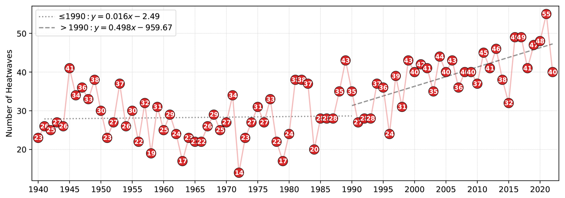
Figure 3 Number of detected heatwave events per year in Western Europe, from 1940 to 2022, identified by the GDBSCAN algorithm (Sander et al., 1998) in ERA5 reanalysis data using the grid cells that exceed the 90th percentile with respect to the 1941–1980 daily maximum temperature climatology. This period precedes the stronger warming trends after 1980 in Europe (Elguindi et al., 2013).

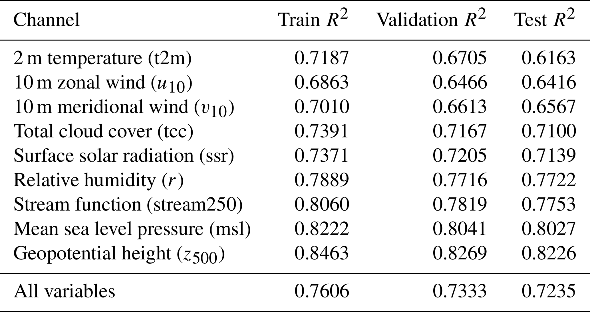
After training the VAE model, we evaluated its reconstruction performance for all climate variables across the training, validation, and test subsets (Table 2). The model achieves overall R² scores of 0.76, 0.73, and 0.72 for the train, validation, and test data, respectively, indicating stable performance and good generalization without signs of overfitting. The highest reconstruction skill is obtained for geopotential height (z₅₀₀) and mean sea level pressure (msl). This agrees with Jézéquel et al. (2018), who found that geopotential height better represents temperature anomalies associated with European heatwaves. Near-surface variables such as 2 m temperature (t2m) and 10 m wind components (u₁₀, v₁₀) show lower scores, reflecting their higher spatiotemporal variability influenced by local surface conditions, which are difficult for the model to capture accurately, considering the coarse spatial resolution of the data and the smoothing of small-scale variability due to the reconstruction loss.

Table 2 R² scores for training, validation, and test subsets. The evaluation is based on input data structured into 1408, 320, and 928 samples for the training, validation, and test sets, respectively, each with nine channels spanning 11 d on a 64×192 grid.

Then, we analyzed the latent-space representations of heatwave samples. Each multivariate heatwave sample was encoded into a 128-dimensional latent space by the VAE. As an intermediate processing step, we first used Principal Component Analysis (PCA) to reduce the dimensionality of all heatwave samples from 1941–2022 to 50 components. Then, we applied the t-SNE algorithm to all heatwave samples to reduce them to two dimensions for visualization of the latent space. This two-step approach is recommended by van der Maaten and Hinton (2008) for t-SNE visualizations of high-dimensional latent spaces to reduce dimensionality and improve efficiency and robustness (Pedregosa et al., 2011). Because these steps involve stochasticity, we fixed the random seed to 42 (Adams, 1979) for PCA, t-SNE, and GMM to ensure consistency across visualization runs.

Figure 4 shows the t-SNE projections for training (1941–1990), validation (1991–2000), test (2001–2022), and combined (1941–2022) samples. During training (from 1941 to 1990, characterized by heatwaves), the VAE was exposed to a larger set of heatwave patterns, which were encoded into a latent space. This spread suggests that there was a wide range of training examples. The validation period shows a consistent distribution with the training periods, suggesting that the model generalizes well with the validation data (1991–2000). Interestingly, the latent space for the test period (2001–2022) shows a ring-like structure with fewer samples in the center and an accumulation toward the positive values of the first component (see Fig. 4c). This shift, compared to previous historical periods, might imply that the nature of heatwaves has changed. As heatwaves become more frequent and extreme (Perkins-Kirkpatrick and Lewis, 2020; Fischer et al., 2021; IPCC, 2021; Russo et al., 2015; Lhotka and Kyselý, 2022; Paçal et al., 2023), the VAE encodes these heatwave samples, which are underrepresented in the training period, into regions of the latent space not occupied by training heatwave samples. This subtle drift is more pronounced in the combined panel in Fig. 4d, suggesting a change in heatwave characteristics during the most recent period (2001–2022).

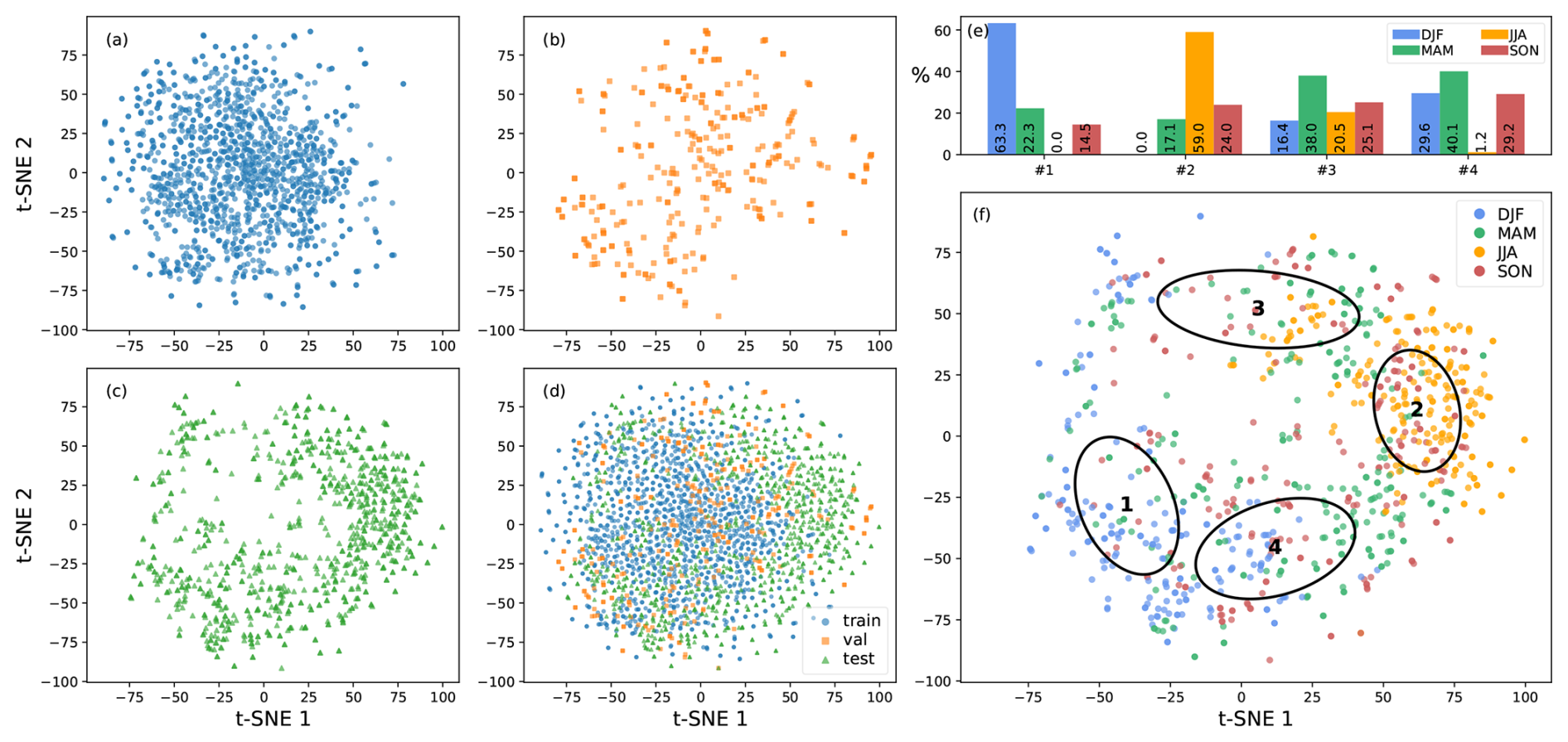
Figure 4 t-SNE representation of the latent space for (a) training (1941–1990), (b) validation (1991–2000), (c) test (2001–2022), and (d) the full period (1941–2022). (e) shows the seasonal distribution of samples within each cluster. (f) displays the t-SNE projection of test-period heatwave samples colored by the season of onset, with ellipses representing the four Gaussian Mixture Model components. Each point corresponds to an individual heatwave event.

To further validate that the observed latent space shifts are not merely artifacts of global warming trends or the data split, we performed a secondary analysis using detrended variables. We quantify distributional shifts using Mahalanobis distance (D), which measures how far the center of the test-period distribution has moved from the training-period distribution in units of standard deviations (De Maesschalck et al., 2000). While we focus on non-detrended data in this study to capture the full thermodynamic intensification of recent heatwaves, the detrended data analysis reveals that statistically significant shifts (p<0.001) persist across all seasons between training (1941–1990) and test (2001–2022) periods (see Appendix Table A2 and Fig. A8). This suggests that, beyond mean-temperature increases, the multivariate structure of atmospheric patterns associated with heatwaves is evolving. Interestingly, in the detrended dataset, summer (JJA) samples exhibit a smaller shift (D=0.34), while winter (DJF) shows a much more robust dynamical evolution (D=1.40). In the non-detrended dataset, summer samples show a higher shift, pointing to a thermodynamical warming (see Appendix Table A3 and Fig. A9). This finding is consistent with recent projections that changes in internal variability and moisture limitations can enhance land-atmosphere feedbacks, particularly in central and northern Europe, thereby altering the nature of extreme events Beobide-Arsuaga et al. (2025). After removing the linear warming trend from the input fields, structural shifts in atmospheric configurations persist across all seasons, indicating that the model captures changes in the multivariate structure of heatwave related variables that are not explained solely by the linear warming trend. However, linear detrending removes only the slow, monotonic component of each input variable, while the residual still contains nonlinear thermodynamic effects and circulation variability (Shaw et al., 2024; Suarez-Gutierrez et al., 2020; Singh et al., 2023; Schumacher et al., 2024). The residual shifts reported here should therefore be interpreted as evidence that the multivariate structure of heatwave-related variables is evolving, rather than as a quantitative attribution to circulation dynamics.

We fitted multiple GMM components to the latent space to identify different clusters of heatwaves. After testing the GMM fits with the Bayesian Information Criterion (BIC) scores and cluster stability across different random initializations, we found that four clusters provide the most robust grouping of test samples (see Appendix Fig. A10 for BIC scores across different components for training, validation, and test periods). While the BIC scores favor simpler models for the training and validation sets, the test set shows a clear minimum at 4 components. This balances model complexity and fits well, as BIC values steadily increase beyond four across all datasets. We color-coded heatwave sample representations in the latent space to interpret the clusters by their corresponding seasons. As shown in Fig. 4f, some clusters are dominated by heatwaves happening at specific seasons (e.g. Cluster #2 with mostly June–July–August (JJA) events), indicating that the model distinguishes between heatwave patterns that align with different seasonal characteristics. While some of this separation could also emerge from individual variables such as air temperature, using multiple variables provides a more complex representation of the atmospheric conditions associated with each cluster. This seasonal structure emerges even though the input data were deseasonalized and standardized. Clusters #2 and #3 in Fig. 4f, respectively, correspond to nearly the same heatwave samples as those shown in the three-component clustering (see Fig. A11 in the Appendix). Since the samples correspond mostly to JJA months in the latent space represented on the right side of the t-SNE plots, this also suggests that these heatwave samples were not very frequent historically, as this aggregation is clearly outside of training period samples, as shown in the combined panel in Fig. 4. Since four components in Fig. 4f provide the possibility of a more detailed analysis for heatwave samples within Cluster #1, i.e. those corresponding to December–January–February (DJF) winter months, while having a similar Cluster #2 and #3 as in the three-cluster case (see Appendix Fig. A11), we chose four GMM components for our further analysis. Similarly, Happé et al. (2024) found that four clusters were optimal for their latent space analysis. Our identified clusters represent then the following seasons: Cluster #1 represents DJF (Sect. 3.2), Cluster #2 represents JJA (Sect. 3.3), Clusters #3 and #4 represent transition seasons March–April–May (MAM) or September–October–November (SON) (Sect. 3.4). To further investigate whether the clustering reflects only seasonal differences or distinct dynamical regimes, we examined the standardized mean anomaly of each variable within the four clusters (Fig. 5). For each variable, we computed the mean standardized anomaly values over all heatwave samples in a cluster. These mean values represent the typical anomaly structure captured by each cluster. Although the clusters align broadly with seasonal timing, their multivariate structures differ beyond temperature intensity. For instance, Cluster #1, representing mainly winter events, exhibits on average weaker positive temperature anomalies but enhanced warm advection (positive v10 values) and reduced solar input (low ssr) (Spanjers et al., 2025). Cluster #2 shows strong positive t2m, r, and z₅₀₀ anomalies typical of intense summer heatwaves (Vautard et al., 2023). Clusters #3 and #4 show mixed transition season features, one dominated by high solar radiation and the other by stronger pressure anomalies (Träger-Chatterjee et al., 2013; Boboc et al., 2025). These differences suggest that latent-space clustering captures distinct dynamical configurations rather than just temperature variability.

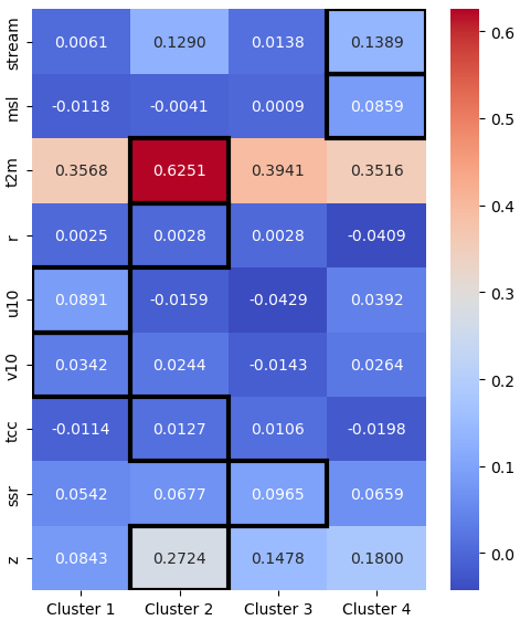
Figure 5 Mean standardized anomaly values for each variable, averaged over all heatwave samples in each latent cluster. The values summarize the typical anomaly patterns represented by the four clusters. Black boxes represent the highest value for each variable.

To analyze the atmospheric patterns before and during heatwaves, we constructed composite representations of heatwave samples for each cluster by selecting the closest 100 samples (in latent space) to each GMM cluster centroid, similar to the procedures described by Rouges et al. (2023) and Happé et al. (2024). Since the entire process, i.e. the encoding of heatwave samples to the latent space by the VAE, the dimensionality reduction via t-SNE, and the GMM clustering, contains randomness, a single sample may be sensitive to random fluctuations. The composite maps provide a more stable representation of atmospheric conditions for each cluster by averaging over the closest samples in the latent space. The anomalies of each variable are displayed for the North Atlantic region (as shown in Fig. 1) for each of the eleven analyzed days (five days before the onset of the heatwave; the onset day of the heatwave, indicated with a broader frame around the graphs; and five days after the onset of the heatwave), and all four identified clusters.

To assess the physical relevance of our VAE-based clustering, we selected several major European heatwaves that have been extensively studied in the literature as case studies. Russo et al. (2015) identified and ranked the top ten most severe European heatwaves between 1950–2014, highlighting events such as the 2003 Western European and 2010 Russian heatwaves as the most severe. Lhotka and Kyselý (2022) expanded on this work by providing an updated catalog of major heatwaves up to 2021. Following these studies, we selected the 2003, 2010, and 2018 heatwaves as case studies to examine whether the VAE latent space captures the known dynamical features of these benchmark events. Due to differences in detection methods, the exact onset dates of heatwaves in our dataset do not always align with those reported in the literature. Therefore, for each target heatwave date defined by Lhotka and Kyselý (2022) (“target date” in Fig. 6), we identified the temporally closest matching event in our dataset (“closest date” in Fig. 6). We then extracted the ten nearest neighbors in the latent space around each closest date to construct composite anomaly maps. This procedure allows us to place these historically significant heatwaves within the structure of the learned latent space and to compare the resulting anomaly patterns directly with those documented in the literature. As shown in Fig. 6, the resulting geopotential height at 500 hPa (z₅₀₀) anomaly maps exhibit similar patterns to those reported by Lhotka and Kyselý (2022). In particular, the 2010 heatwave shows characteristic strong positive z₅₀₀ anomalies over western Russia; the 2003 event exhibits a ridge over central Europe; and the 2018 heatwave displays height anomalies over Scandinavia. These spatial features closely match the patterns reported in Fig. 3 of Lhotka and Kyselý (2022), demonstrating that the VAE organizes these events in a way that is consistent with established dynamical interpretations.

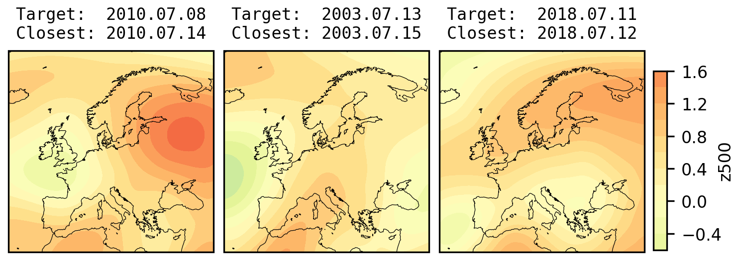
Figure 6 Geopotential height at 500 hPa (z₅₀₀) anomaly maps for three historically significant European heatwaves: 2010, 2003, and 2018. The target dates correspond to the heatwave onset dates defined by Lhotka and Kyselý (2022), while the closest dates refer to the temporally nearest matching events detected in our dataset using the GDBSCAN algorithm. For each event, composite maps are constructed by averaging the 10 latent-space neighbors closest to the selected onset date. The spatial domain in this figure is cropped to match that used by Lhotka and Kyselý (2022), for consistency, although other figures in this study use a broader domain.

3.2 Cluster no. 1

Using the composite maps, we found that four heatwave clusters exhibit distinct atmospheric patterns across seasons. The composite anomaly maps for each of the nine atmospheric variables across all four heatwave clusters are presented in Figs. 7–15, showing the temporal evolution from five days before to five days after the heatwave onset. In Figs. 7 and 8, Cluster #1 exhibits a circulation structure that is topologically similar to the UK High cluster in Happé et al. (2024) and the omega block in Rouges et al. (2023) for the onset day of the heatwaves, persistent anticyclonic anomaly centered over the British Isles and Western Europe, with positive geopotential height anomalies, suppressed cloud cover, and warm advection from the Atlantic. This comparison refers to the dynamical structure of the circulation pattern, not to its seasonal context or absolute temperature anomaly levels. Cluster #1 is dominated by winter events and contains no summer heatwaves (Fig. 4e) and accordingly shows weak positive 2 m temperature anomaly (Fig. 5). Because our heatwave sample detection method is seasonal threshold-based (Sect. 2.2), an event in this cluster represents anomalous warmth relative to its own seasonal climatology, i.e. a winter warm spell, rather than absolute heat comparable to summer. While Happé et al. (2024) found this UK high pattern in summer (JJA) months and Rouges et al. (2023) found this pattern in extended summer (May to September) months, our analysis, which uses standardized anomalies relative to each calendar day's local climatology, reveals that structurally analogous circulation configurations also drive anomalous warmth during winter months relative to the winter baseline. This is consistent with previous studies documenting that winter warm spells over Europe are associated with positive geopotential height anomalies and anticyclonic blocking, as shown in Fig. 15 (Tomczyk et al., 2019; Leach et al., 2021).

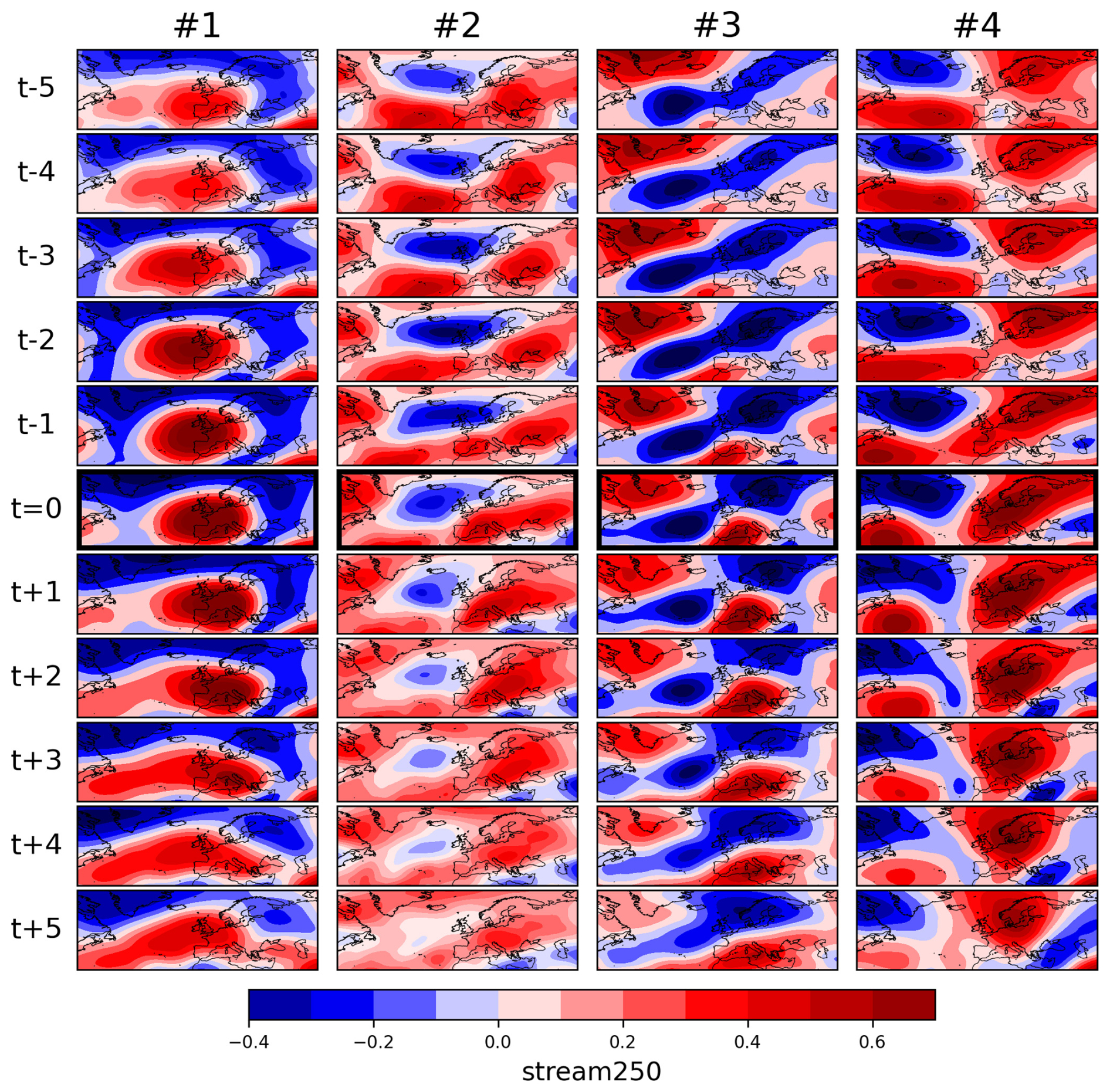
Figure 7 Composite map for standardized stream function anomaly at 250 hPa (stream250) across t±5 d for each GMM cluster identified in Fig. 4f. Rows show Cluster #1 to #4, and each row corresponds to the cluster average of the n=100 heatwave samples closest to the respective GMM centroids. Time progresses from top to bottom, centered on the heatwave onset date (t=0), as shown in the sixth row, and is emphasized with a broader frame.

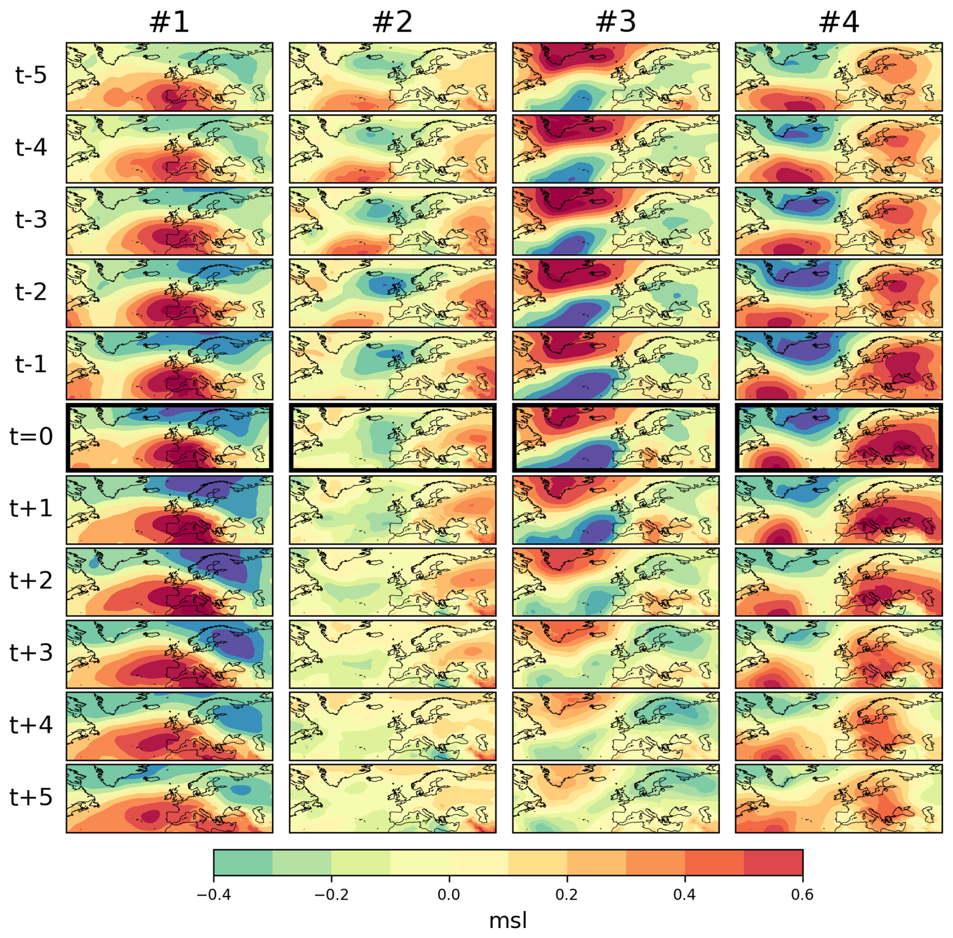
Figure 8 Same as Fig. 7, but for standardized mean sea level pressure (msl) anomaly.

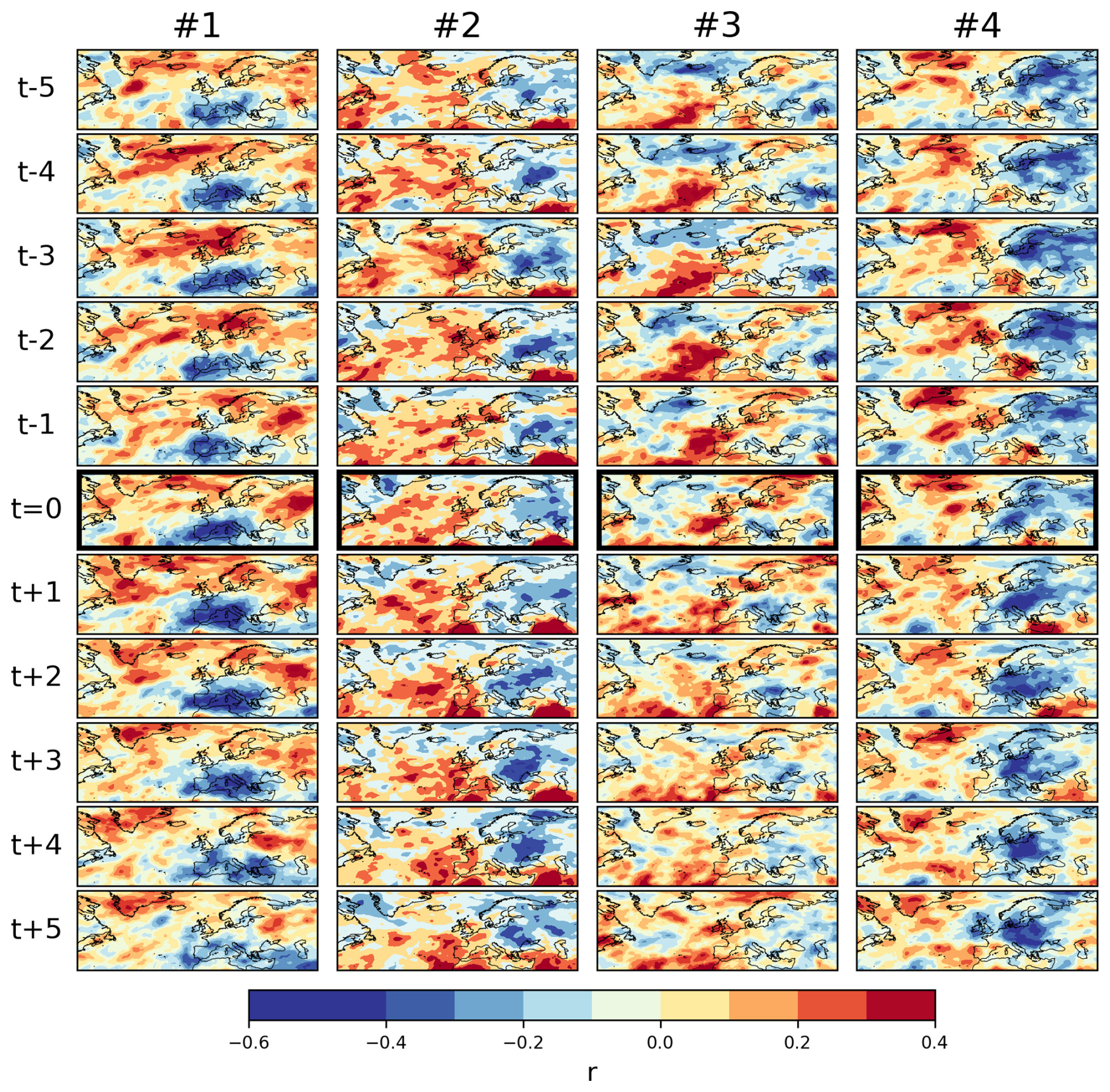
Figure 9 Same as Fig. 7, but for standardized relative humidity (r) anomaly.

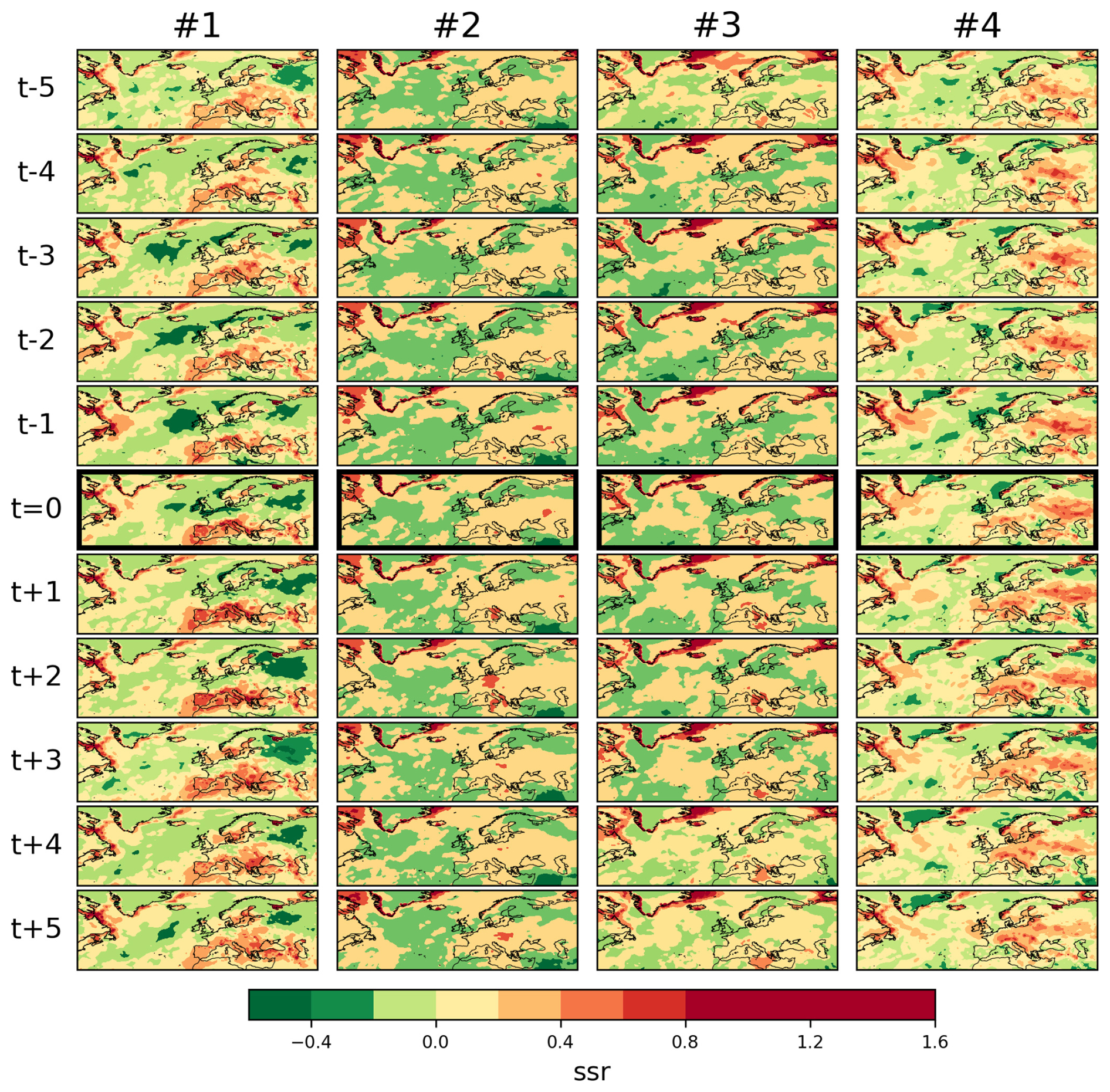
Figure 10 Same as Fig. 7, but for standardized sum surface net solar radiation (ssr) anomaly.

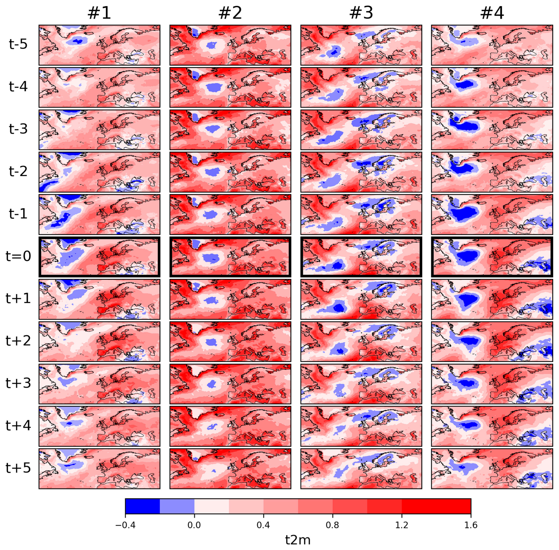
Figure 11 Same as Fig. 7, but for standardized maximum 2 m temperature (t2m) anomaly.

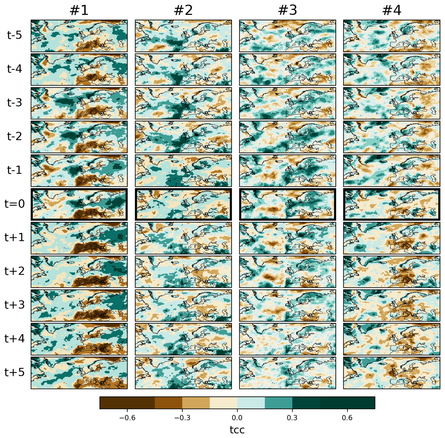
Figure 12 Same as Fig. 7, but for standardized total cloud cover (tcc) anomaly.

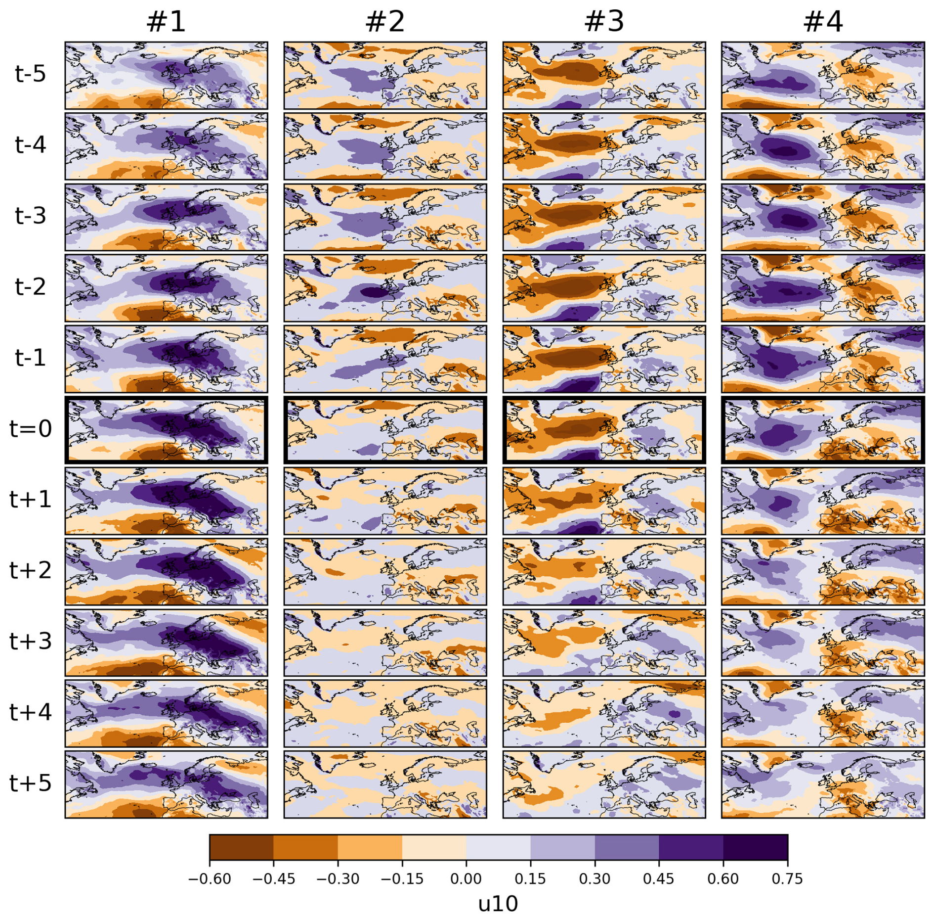
Figure 13 Same as Fig. 7, but for standardized 10 m eastward wind component (u₁₀) anomaly.

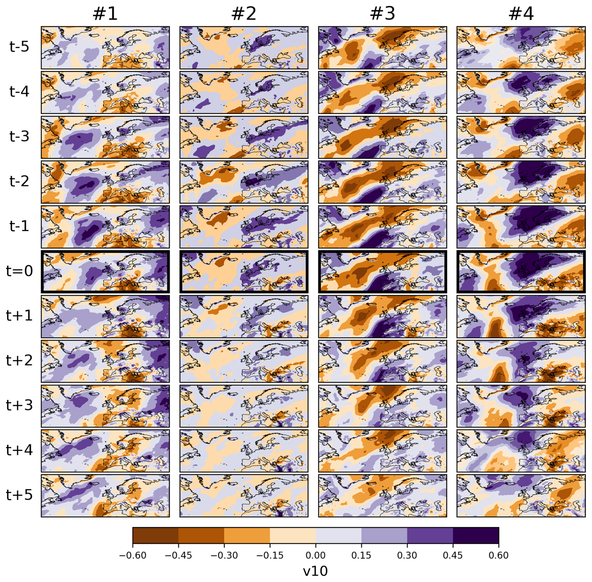
Figure 14 Same as Fig. 7, but for standardized 10 m northward wind component (v₁₀) anomaly.

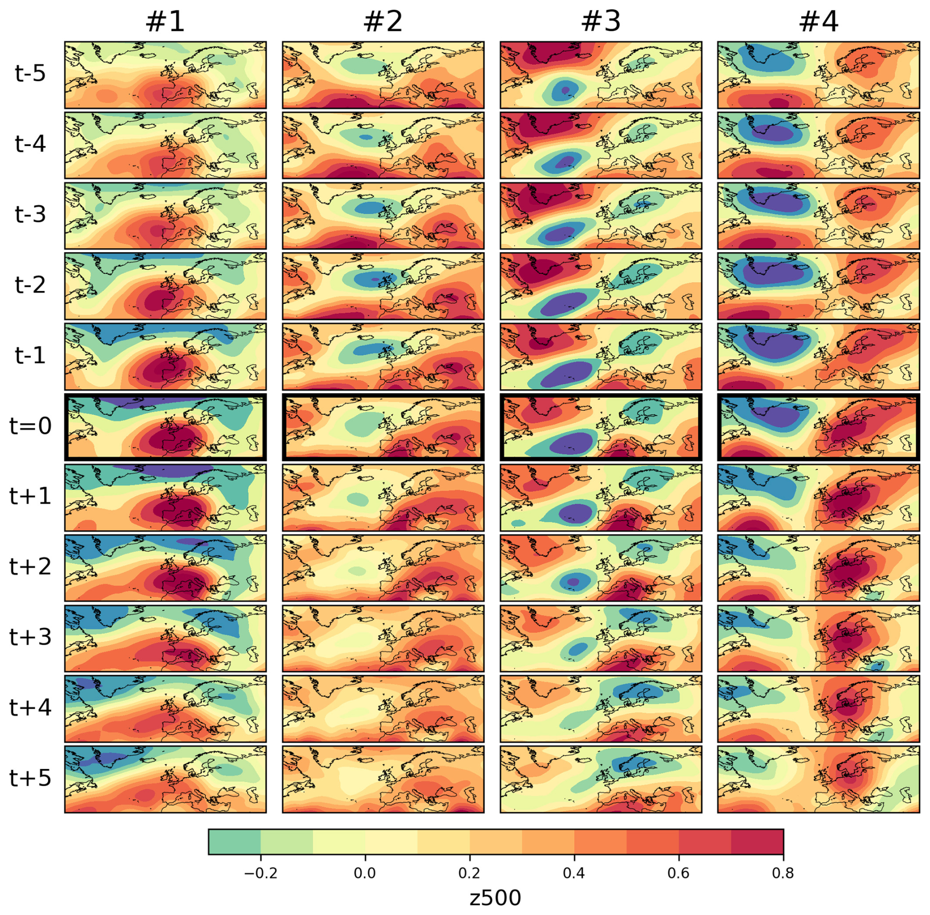
Figure 15 Same as Fig. 7, but for standardized geopotential height at 500 hPa (z₅₀₀) anomaly.

As the extreme event progresses (the days after the onset), these geopotential height at 500 hPa (z₅₀₀) anomalies begin to disperse eastward across the North Atlantic, as shown in Cluster #1 in Fig. 15. Tomczyk et al. (2019) also demonstrated this in their study: anomalies in geopotential height begin to develop over the North Atlantic and move towards Europe, where they intensify as they traverse the continent. This pattern of dispersion is also evident in Fig. 11: the positive maximum temperature anomalies associated with winter heatwaves are initially concentrated over Western Europe, gradually weakening and dissipating in a similar manner following the onset of the heatwave events in Cluster #1. These patterns are also consistent with findings from previous studies where heatwaves in north-west Europe are typically found to be related to blockings (Carril et al., 2008; Zschenderlein et al., 2020). This blocking is also accompanied by a positive (negative) anomaly in the zonal wind (u₁₀) component at the north (south), and a dipole structure with positive (negative) anomalies to the west (east) in the meridional wind (v₁₀) (see Cluster #1 in Figs. 13 and 14). Together, these features point to a blocking structure with enhanced atmospheric stagnation, consistent with an anti-cyclonic flow (Kautz et al., 2022), and advection of warm-moist air from the Atlantic (Spanjers et al., 2025). This blocking system helps create and maintain unusually warm weather, which is associated with clear skies, as shown in Cluster #1 in Figs. 10 and 12. The lack of cloud cover, indicated by negative anomalies in the total cloud cover (tcc) variable, for Cluster #1 over Southern Europe and the Mediterranean in Fig. 12, allows more solar radiation to reach the Earth's surface, especially during the build-up of the heatwaves (days t−5 to day 0), where these negative anomalies are more pronounced. The positive anomalies in surface net solar radiation (ssr), as shown in Fig. 10, become more distinct especially after the heatwave event has started, creating a feedback loop that brings further warm and dry air into the region, as shown with negative relative humidity (r) anomalies located over Europe in Fig. 9 during the onset. During the days after the onset, the negative anomaly for relative humidity tends to move eastward towards the Middle East.

3.3 Cluster no. 2

Cluster #2, which corresponds to mostly summer heatwaves, as shown in Fig. 4f, exhibits a similar atmospheric pattern to the southern European cluster (SE) in Rouges et al. (2023). As shown in Fig. 7, stream function at 250 hPa (stream250) shows a broad negative anomaly over the North Atlantic, expanding from Greenland to Scandinavia, while a larger positive anomaly block is observed from the central North Atlantic to Russia from t−5 d before the heatwave onset. Similarly, a continuous ridge pattern in geopotential height at 500 hPa (z₅₀₀) is detectable. It is accompanied by a positive anomaly in zonal wind component, as shown in Fig. 13, up to t+3 d, and positive anomalies in the meridional wind component, especially from t−1 d in the build-up period of heatwaves, as shown in Fig. 14. These anomalies point to greater heat transfer from lower latitudes to Europe. Positive anomalies in geopotential height at 500 hPa (z₅₀₀) over the Subtropical North Atlantic region start t−5 d before the onset, and later sweep into Central Europe during the progression of heatwaves. This finding is similar to that reported by Tomczyk et al. (2019), who showed that warm spells in winter months are associated with positive geopotential height anomalies at 500 hPa (z₅₀₀) over Central Europe. After the onset, the positive anomaly ridge in stream function at 250 hPa (stream250), stretching from central North Atlantic to Russia, surrounds the North Atlantic trough, and extends to North America through to the Arctic during the progression of heatwaves, as seen in Cluster #2, from t=0 to t+5 d, in Fig. 7, while the negative anomalies over North Atlantic dissipates. A persistent negative mean sea level pressure (msl) anomaly occurs over the British Isles during the build-up period of these heatwaves, where it later gives way to a positive anomaly over Russia up to t+3 d, as shown in Fig. 8. As these persistent patterns start to dissipate after the onset of the heatwave, cloud-free skies and a stagnant atmosphere prevail. This is indicated by expanding negative anomalies in total cloud cover (tcc) over Europe and Russia, and near-zero wind speed anomalies, as shown in Figs. 12–14, respectively. The positive anomalies in relative humidity (r) over the North Atlantic during the build-up period of heatwaves gradually spread into Western Europe, while the zonal wind component shows positive anomalies during the same period. This brings more humid, warm air to Europe, creating positive anomalies in relative humidity (r) over Western Europe on the onset date and merging with anomalies over the Middle East during the heatwave, as shown in Fig. 9. Simultaneously, positive temperature anomalies propagate northeast towards central Europe as the heatwave progresses, as shown in Fig. 11. On the other hand, a clear negative anomaly pattern over the North Atlantic in 2 m temperatures (t2m) is observed during the build-up and progression of the heatwaves. This negative anomaly pattern over the North Atlantic is consistent with results described by Krüger et al. (2023), Bischof et al. (2023), and Lipfert et al. (2024), who showed that colder-than-usual North Atlantic sea surface temperatures (SSTs) with a negative tendency are associated with persistent negative anomalies. These conditions promote a deep North Atlantic trough and the subsequent formation of a European ridge, which in turn favors stronger and longer-lasting heatwaves as well as a shift toward positive summer temperature anomalies over Europe (Krüger et al., 2023). These interacting atmospheric mechanisms help explain why the latent space representations of summer heatwave samples (see Fig. 4) are distinctly clustered and separate from the rest of the dataset. The isolation of this cluster underscores that summer heatwaves are not driven by simple linear temperature increases, but by a highly nonlinear interplay between specific dynamical configurations (like the deep North Atlantic trough) and intense thermodynamic processes. As heatwaves intensify and high temperatures rise more rapidly in Europe and other mid-latitude regions (Beobide-Arsuaga et al., 2025; Perkins-Kirkpatrick and Lewis, 2020; Bischof et al., 2023; Paçal et al., 2023), enhanced land-atmosphere coupling and moisture deficits physically alter the atmospheric state (Chen et al., 2026; Shaw et al., 2024). Since the VAE is sensitive to these complex, coupled multivariate structures, recent extreme summer events diverge sharply from the historical distribution learned during training.

3.4 Clusters nos. 3 and 4

Clusters #3 and #4 primarily correspond to heatwaves in the transition seasons, occurring mainly during MAM or SON. The separation of these two clusters directly demonstrates that the VAE's latent space captures distinct physical atmospheric configurations, rather than merely sorting events by the season. Although both clusters occur during the same transition months, they represent fundamentally different dynamical regimes. Cluster #3 is driven by a thermodynamic pathway dominated by enhanced solar radiation and clear skies, while Cluster #4 is linked to stronger large-scale pressure anomalies and advection. Similarly, autumn heatwaves are associated with high-pressure anomalies over western and southern Europe, leading to persistent warm conditions (Boboc et al., 2025). Träger-Chatterjee et al. (2013) found that enhanced solar irradiation during late winter and spring is associated with the development of warm conditions in the coming months. Even though it is not possible to assign these clusters to certain seasons as we could do with the first two clusters, Cluster #4 shows some similarities in anomaly patterns in certain variables with Cluster #1, such as (1) 2 m temperature (t2m), where both show a negative–positive–negative anomaly tripole across the North Atlantic–Europe–Russia domain; (2) mean sea level pressure (msl), where both show negative anomalies closer to Arctic while having positive anomalies over Europe, (3) stream function at 250 hPa (stream250), where both show negative anomalies over Greenland with positive anomalies over Europe. These similarities could explain why the GMMs in Figs. A11 and 4f, with three or four components, consistently identify the same seasonal clusters (#2 and #3), while Clusters #1 and #4 are either merged or separated depending on the number of components. Four components are used in our study to better understand the differences in the characteristics of heatwave clusters.

Although Clusters #3 and #4 are both associated with transition seasons, they exhibit nearly opposite atmospheric anomaly patterns in several key climate variables. This separation in the latent space indicates the model's capacity to distinguish distinct physical mechanisms operating within the same time of year. For instance, in Fig. 15, Cluster #3 displays a positive geopotential height at 500 hPa (z₅₀₀) anomaly over Greenland and negative anomalies over the North Atlantic extending into Scandinavia, a pattern consistent with Greenland blocking events which are known to cause European heatwaves (Kornhuber et al., 2017). Conversely, Cluster #4 shows the opposite, i.e. negative anomalies over Greenland and positive anomalies over the North Atlantic–Scandinavia sector. This creates a contrasting tripole structure during the heatwave build-up phase, which then evolves into opposite-sign anomalies over Scandinavia as the events progress. Likewise, the zonal (u₁₀) and meridional (v₁₀) wind component anomalies show opposing dipole structures between the two clusters, as shown in Fig. 13 and 14. Cluster #3 shows a positive meridional wind (v₁₀) anomaly over the Canaries, t−5 d before the onset, and slowly becomes more prominent as the anomaly expands towards Europe during the event's progress. Since this positive anomaly of wind becomes more prominent as the onset date approaches, increasing wind anomalies enhance the advection of warm air from the south, as shown in Fig. 11.

On the other hand, the wind components for Cluster #4 exhibit anti-cyclonic flow with positive (negative) anomalies over the western North Atlantic (Canaries) during the build-up shown in Figs. 13 and 14, which carries warm air through the North Atlantic, as shown in temperature anomalies in Fig. 11. Cluster #3 is characterized by an elongated trough in stream function at 250 hPa (stream250) extending from the east coast of Canada towards Scandinavia, with a ridge over Greenland. Conversely, Cluster #4 exhibits an inverse pattern with a trough over Greenland, and two ridges are located over the central North Atlantic and Scandinavia, as shown in Fig. 7, showing similarities with the North Atlantic Low cluster in Happé et al. (2024). This elongated trough in Cluster #3 persists across all analyzed heatwave time steps, while the ridge over the central North Atlantic in Cluster #4 dissolves as the event progresses. Furthermore, while heatwave Cluster #3 is accompanied by positive relative humidity (r) anomalies over the Eastern subtropical North Atlantic during the build-up and over Europe following the onset, Cluster #4 exhibits negative relative humidity (r) anomalies over Central Europe and Russia (see Fig. 9). Recent studies also highlight that the accelerated decline of Arctic sea ice since the 2000s has contributed to a shift toward a dipole-like atmospheric circulation mode, resulting in more heatwaves in Europe (Zhang et al., 2020; Lee et al., 2025). These enhance warm-air advection from the North Atlantic and favor soil drying over Europe, supporting the contrasting atmospheric-variability anomalies observed between Clusters #3 and #4.

4 Discussion and Conclusions

Heatwaves are expected to intensify and occur more frequently, particularly in Western Europe, where recent extremes have exceeded model projections (Perkins-Kirkpatrick and Lewis, 2020; Russo and Domeisen, 2023; Schielicke and Pfahl, 2022; Paçal et al., 2023; Vautard et al., 2023; Patterson, 2023; McKinnon et al., 2024; Kornhuber et al., 2024). However, these dynamics are not yet fully understood due to the complex interactions between multivariate spatiotemporal variables and the limited availability of labeled data, making unsupervised learning a promising approach (Van Oldenborgh et al., 2022; Barriopedro et al., 2023; Ruff et al., 2021). This study aims to investigate the interplay and temporal evolution of different atmospheric variables in their contributions to heatwaves in Western Europe. To achieve this, we employed a Variational Autoencoder (VAE) and interpreted the different data clusters, identified by a Gaussian Mixture Model (GMM), in the latent space. Our work builds directly on Happé et al. (2024), but extends it in several important ways. While their study focused on summer heatwaves in the KNMI-LENTIS ensemble dataset, our analysis uses ERA5 reanalysis data, encompasses nine variables, spans all seasons, and incorporates a longer heatwave sample window (11 d). We also analyze historical and recent periods separately to assess how heatwave samples are represented in the VAE latent space across the two periods. These patterns were subsequently analyzed to gain a deeper understanding of the development and progression of heatwaves across all seasons, including summer, winter, and transition periods. By training the VAE on year-round heatwave samples, we captured a comprehensive view of the atmospheric dynamics associated with various heatwave events. Our VAE analysis identified several distinct heatwave regimes from the ERA5 dataset, each associated with characteristic atmospheric patterns and seasonal preferences.

While we trained the VAE model with year-round heatwave samples from ERA5, the composite maps of the resulting heatwave clusters reveal atmospheric patterns consistent with previous studies, which typically considered only summer months (Carril et al., 2008; Horton et al., 2015; Rouges et al., 2023; Krüger et al., 2023; Bischof et al., 2023; Happé et al., 2024). We observed a similar pattern in Cluster #1 to the UK High cluster described by Happé et al. (2024) and the omega block reported by Rouges et al. (2023), although our analysis considered year-round heatwave samples. In contrast, those studies focused only on summer events. As explained before, our choice of four Gaussian components for our analyses enables a more nuanced analysis of heatwave regimes and enhances the interpretability of the latent space. Each of the four identified groups captures distinct atmospheric conditions in different variables analyzed, with well-defined patterns leading to the onset of the heatwave and their subsequent progression, as illustrated in the composite anomaly maps in Figs. 7–15. For example, anomalies in relative humidity (r) in Fig. 9 highlight contrasting patterns between seasonal heatwaves: Cluster #1, associated with winter heatwave samples, exhibits a pronounced negative relative humidity (r) anomaly over Western Europe and the Mediterranean, whereas Cluster #2, dominated by summer heatwaves, shows a positive relative humidity (r) anomaly following the onset. This distinction is consistent with previous studies, which indicate that humid summer heatwaves are highly dangerous and are intensifying under climate change (Russo et al., 2017; Dong et al., 2024; Wang et al., 2024). The total cloud cover (tcc) shows a distinct negative anomaly starting from t−5 d and strengthening during the progression of winter heatwaves over Southern Europe, causing a positive anomaly in surface net solar radiation (ssr) a couple of days later, which brings more heat to Western Europe, as seen in Cluster #1 (Fig. 10). Meanwhile, positive anomalies in total cloud cover (tcc) are observed before the onset of summer heatwaves in Cluster #2. Still, they gradually transition into negative anomalies in total cloud cover (tcc) over Central Europe as the heatwave evolves (Fig. 12). Despite the data being standardized, the VAE organizes heatwave samples into clusters that align with seasonal differences, suggesting that seasonal signals are embedded in the atmospheric patterns of the test period. We note that the persistence of seasonal grouping despite year-round, deseasonalized, and standardized inputs indicates that the multivariate circulation structure of heatwaves differs systematically across seasons. The clearest illustration is the pair of transition-season Clusters #3 and #4, which contains same seasonal samples (MAM and SON) yet display near-opposite z₅₀₀, wind, and humidity structures, confirming that the clustering separates dynamical regimes and not merely calendar months.

Our statistical validation confirms that these latent space shifts are not mere artifacts of the temporal split or thermodynamic trends. Hotelling's T² tests reveal highly significant temporal shifts (p<0.001) across all seasons in both detrended and non-detrended data. The contrasting seasonal responses to detrending indicate that the removable linear component of the latent-space shift is largest in summer, consistent with the strong warming-driven intensification of recent summer heatwaves (Mazdiyasni et al., 2019; Beobide-Arsuaga et al., 2025), whereas substantial shifts persist in the other seasons once the linear trend is removed. While the warming-related component dominates the summer heatwave separation signal, the robust shifts maintained in other seasons demonstrate that the VAE successfully captures genuine structural changes in atmospheric dynamics that were not present during the training period. This finding aligns with previous studies, which have shown that climate change impacts seasonal cycles (Wang et al., 2021; Paçal et al., 2023). Similarly, Beobide-Arsuaga et al. (2025) showed that forced changes in internal variability under global warming are projected to further intensify summer heatwaves in central and northern Europe, highlighting that frequent moisture limitations in these regions enhance land-atmosphere feedbacks, increasing both the intensity and variability of heatwaves.

This study highlighted the potential of machine learning methods to improve our understanding of heatwaves. By using a VAE, we uncovered a data-driven classification of heatwave events that not only aligns with known atmospheric circulation regimes from previous studies but also reveals their seasonal and dynamical characteristics from several days before the onset of the heatwave until several days after. Our results showed that the VAE's latent space effectively captures key atmospheric patterns previously linked to extreme heat events, such as blocking highs, omega blocks, and persistent ridges, similar to those identified by Happé et al. (2024) and Rouges et al. (2023).

The VAE's ability to identify these distributional changes in the latent space without supervision suggests that unsupervised learning techniques can be a valuable tool for identifying non-stationary shifts in high-dimensional atmospheric states (Behrens et al., 2022; Shamekh et al., 2023; Mooers et al., 2023; Camps-Valls et al., 2025).

Despite these promising results for identifying heatwaves and their underlying atmospheric conditions, several limitations of the current approach must be acknowledged. First, we adopt a percentile-based threshold for detecting heatwave sample onset dates using 2 m temperature anomalies over Western Europe. However, there is no universally accepted definition of heatwaves (Barriopedro et al., 2023; Boni et al., 2023). Alternative heatwave indices could yield different heatwave samples and thus different atmospheric patterns. Second, while we used variables related to atmospheric heatwaves, other potentially relevant drivers of heatwave dynamics may not be represented. As a result, the clusters we identify should be interpreted as emerging from the chosen subset of variables rather than from the full spectrum of processes affecting heatwaves. In addition, ERA5 itself has known uncertainties (Soci et al., 2024). Future work could improve this by also analyzing other variables to capture additional feedback processes. Third, the VAE is trained on historical heatwaves (1941–1990) and tested with recent heatwaves. While this was a deliberate choice to investigate how recent heatwaves differ from historical heatwaves, it assumes that the latent representation learned from the historical period can adequately model unprecedented patterns arising from climate change. Similarly, the use of linear detrending on the input data cannot isolate nonlinear soil moisture-atmosphere feedbacks, whose competing thermal warming and moisture depletion effects drive spatially divergent responses of heat extremes (Chen et al., 2026; Lindenlaub et al., 2026), nor disentangle the forced response from internal variability (Shaw et al., 2024). Furthermore, the VAE approach introduces some uncertainties due to the choices in model architecture. Key hyperparameters (such as the dimensionality of the latent space, learning rate, batch size, and the number of layers) can significantly influence training outcomes and the structure of the latent space. In addition, dimensionality reduction using PCA and t-SNE, followed by clustering with GMM, further influences how heatwave events are grouped in the latent space, as all these steps involve stochastic elements. Finally, the VAE reconstructions tend to smooth out extremes, and the use of composite maps that average 100 nearest latent samples, while reducing randomness and providing a more stable representation of atmospheric conditions, may mask variability within clusters. These limitations highlight that the VAE clustering approach is one possible data-driven analysis of atmospheric dynamics associated with heatwaves, rather than a definitive classification.

An open question concerns whether the atmospheric patterns identified before heatwave onsets also appear during periods without subsequent temperature extremes. We computed the mean bias between the composite fields of the summer cluster center and 11 d running window samples from all summer days from 2015 to 2021 for each variable. This approach tests whether these circulation patterns arise exclusively before heatwaves. Our preliminary results did not show a clear predictive signal, suggesting that these large-scale configurations can occur without always leading to a heatwave. Future work could investigate the potential predictive value and improve understanding of the physical mechanisms linking circulation anomalies to heatwave development. Another possible approach could be to enhance the model's ability to analyze various types of extreme events by incorporating additional variables, such as soil moisture, vegetation indices, or extreme indices. Furthermore, applying the VAE model to CMIP6 climate simulations (Eyring et al., 2016) to evaluate how well climate models capture historical heatwave patterns compared to reanalysis data could provide valuable insights on model biases and help to bridge the gap between observational and model-based understanding of extreme events in a warming climate (Domeisen et al., 2022; Kornhuber et al., 2024; Barriopedro et al., 2023; Brunner and Voigt, 2024). These insights are particularly relevant for climate change adaptation and mitigation efforts (IPCC, 2021), as heatwaves pose serious risks to both environmental systems and human health (Mora et al., 2017b).

Appendix A: Details for the Variational Autoencoder

VAEs, like other deep learning models, require several design choices before training. These hyperparameters determine how the model performs, such as the learning rate (how it adjusts its parameters during each training iteration), the batch size (how many samples it uses in each iteration), and the hidden layer and latent space sizes (how complex its internal representations are). Since these settings strongly affect the performance of the model reconstruction, we conducted a grid search over a range of hyperparameters, including learning rates ([0.0001, 0.001, 0.01]), batch sizes ([8, 16, 32, 64]), hidden layer dimensions ([64, 128, 256]), and latent space sizes ([64, 128, 256]). The model performance improves substantially with increasing hidden dimension, as shown in Fig. A12. Based on the model's performance on the unseen validation data, we selected a learning rate of 0.001, a batch size of 32, a hidden layer size of 256, and a latent space size of 128. These choices provided a good balance between reconstruction accuracy, latent-space simplicity, and computational efficiency.

The encoder processes the input with four layers of 3D convolutions with Max Pooling layers across the variable, time, and spatial dimensions (see Table A1). Likewise, Happé et al. (2024) used a similar architecture and latent space size. By using 3D convolutions, the model captures interactions across time and space simultaneously. It gradually reduces the spatiotemporal heatwave data in the encoder. From the encoded representation, the model estimates the parameters of a latent distribution using the reparameterization trick (Kingma and Welling, 2019). Sampling from this distribution yields a 128-dimensional latent vector that serves as the compressed representation of each heatwave event. The decoder, consisting of four layers of 3D transposed convolutions with corresponding unpooling operations to restore the original input dimensions, reconstructs the heatwave sample from its latent-space representation. By minimizing the reconstruction loss between the original input and the decoder output, the model learns to optimize its parameters. The encoder-decoder architecture is symmetric and fully convolutional, preserving spatiotemporal locality throughout the encoding and decoding process, as described in Table A1.

Table A1 Architecture of the VAE model. Each row shows the layer name, the output tensor size after the operation, the number of input and output filters (where applicable), the convolution or transpose convolution kernel size, the applied padding, and the stride. The output has dimensions corresponding to variables (9), days (11), latitude (64), and longitude (192). The encoder compresses the input, and fully connected (FC) layers map the flattened encoder output to the latent space. In VAEs, the latent space is sampled from a Gaussian distribution. Two separate FC layers generate the mean (FC_μ) and standard deviation (FC_σ) vectors that parameterize the latent Gaussian distribution. After sampling from the latent space, the data are reshaped and passed into the decoder to reconstruct the input.

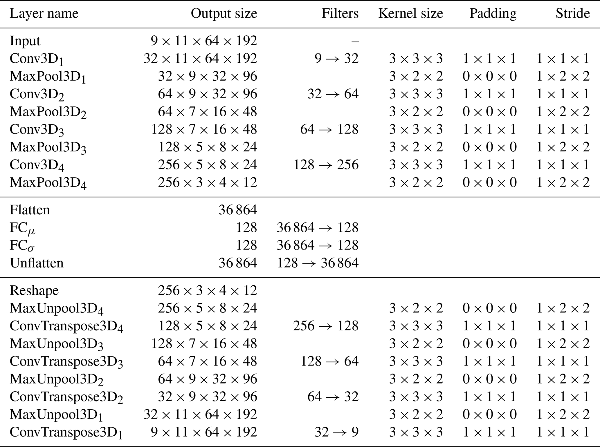
Table A2 Temporal shift analysis of seasonal embeddings in detrended data (1941–1990 vs. 2001–2022). Samples are grouped by seasons based on their dates, not by GMM assignment. Different total sample counts compared to non-detrended data (Table A3) result from independent heatwave detection on detrended temperature fields.

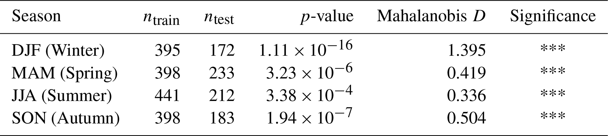
* p<0.05, ** p<0.01, *** p<0.001

Table A3 Temporal shift analysis of seasonal embeddings in non-detrended data (1941–1990 vs. 2001–2022). Samples are grouped by seasons based on their dates, not by GMM assignment.

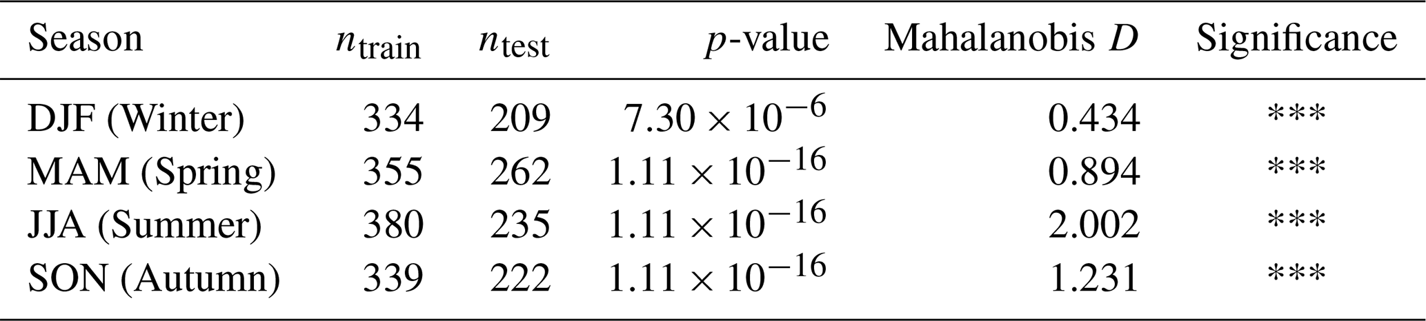
* p<0.05, ** p<0.01, *** p<0.001

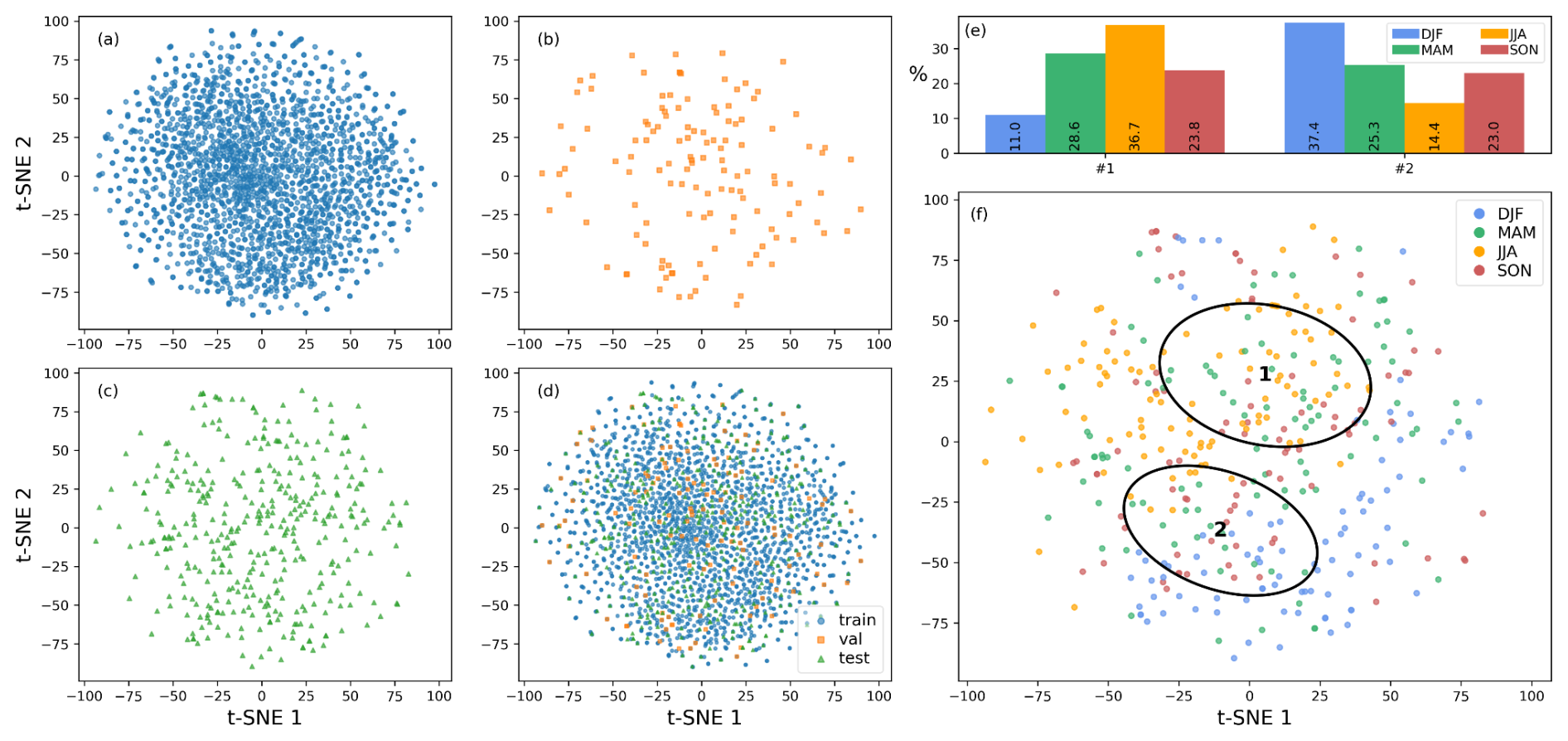
Figure A1 t-SNE representation of the latent space with random-split data ($\mathrm{0.8}/\mathrm{0.05}/\mathrm{0.15}$). Following our workflow (testing with more than 2 components), a 2-component GMM provided the best fit, as it was closest to a single Gaussian distribution and thus better captured the smooth latent-space structure. While this approach provides a smoother latent space, summer heatwaves still accumulate more closely together. This confirms that the clustering is not simply an artifact in the time series but reflects consistent structural patterns across periods.

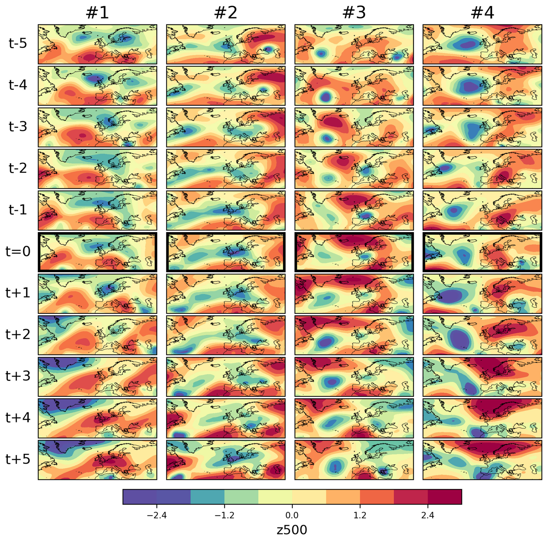
Figure A2 1-sample composite map.

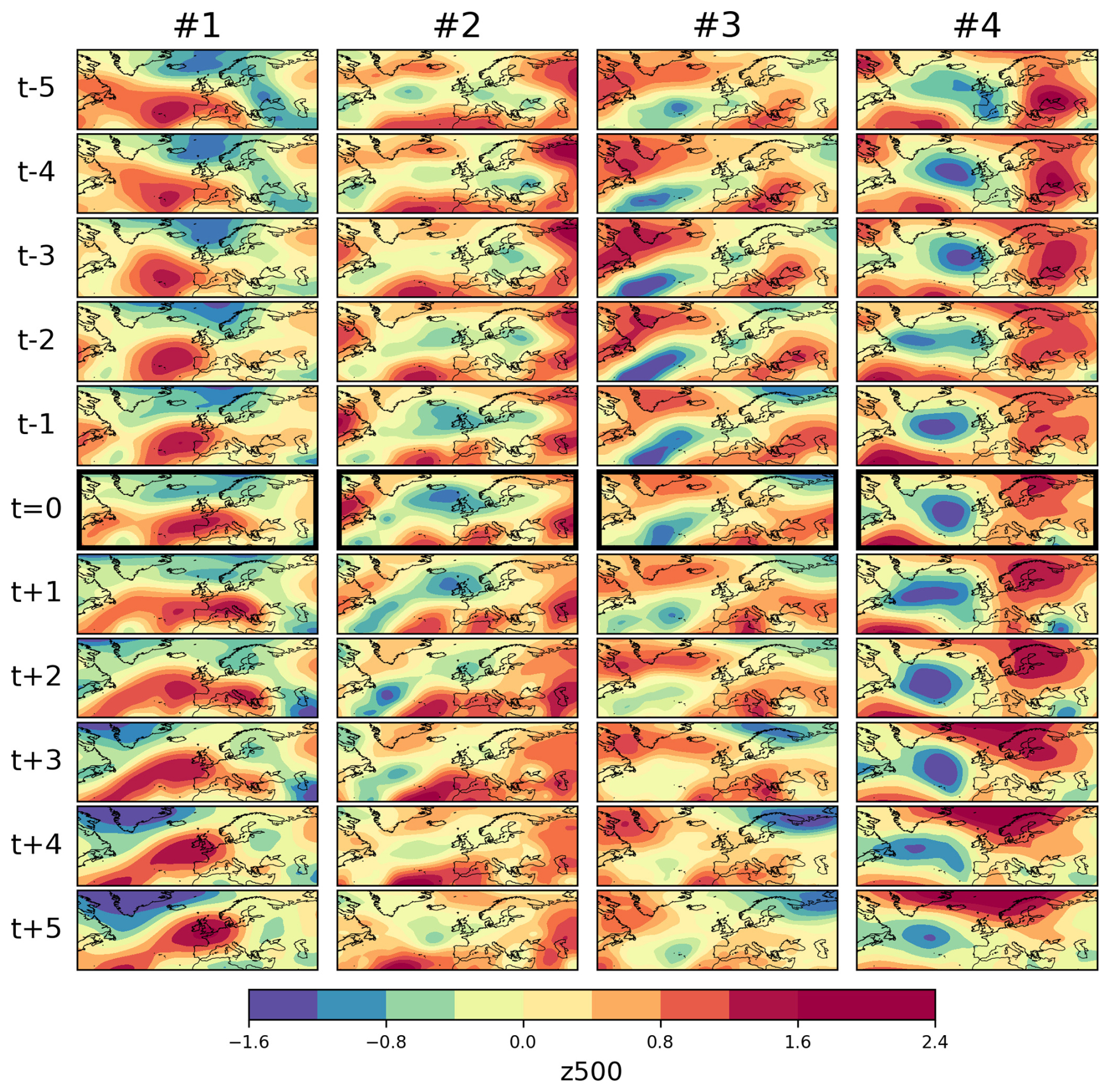
Figure A3 5-sample composite map.

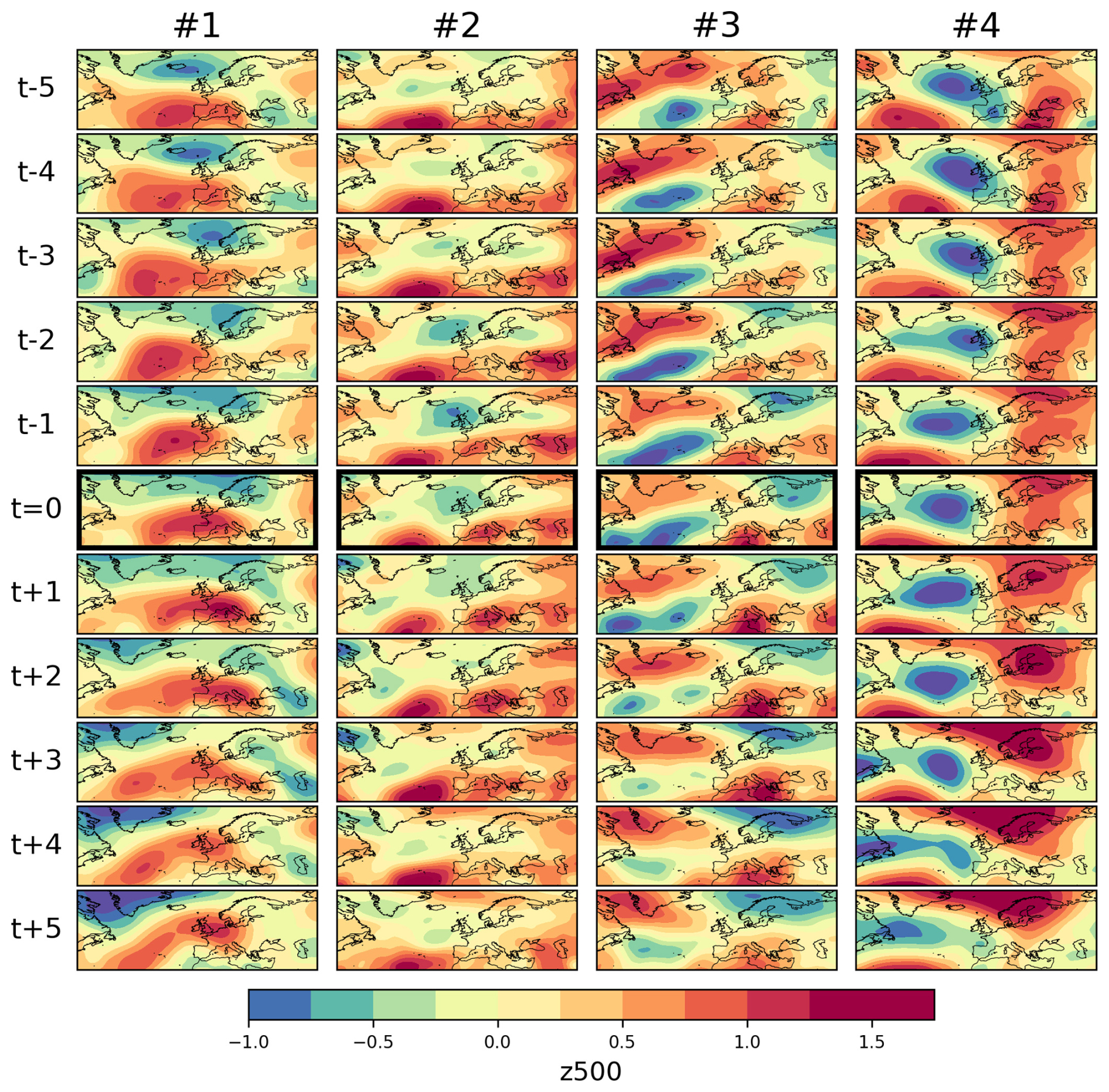
Figure A4 10-sample composite map.

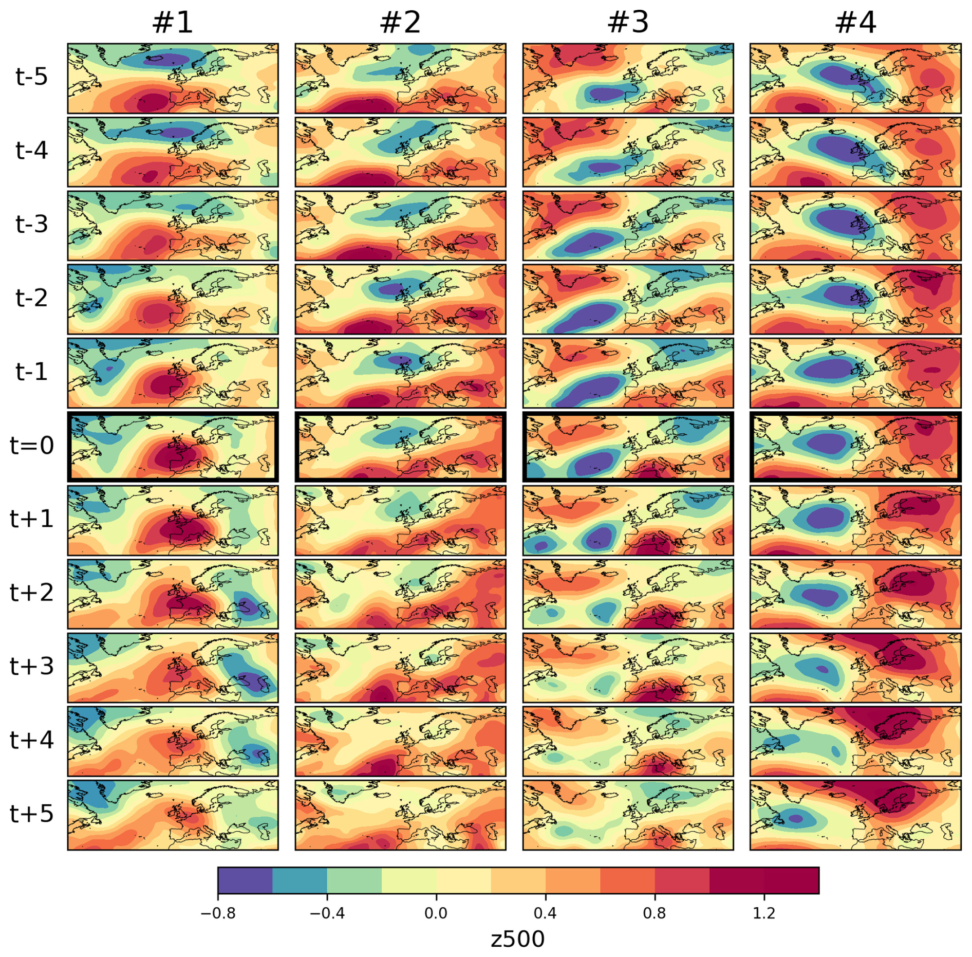
Figure A5 20-sample composite map.

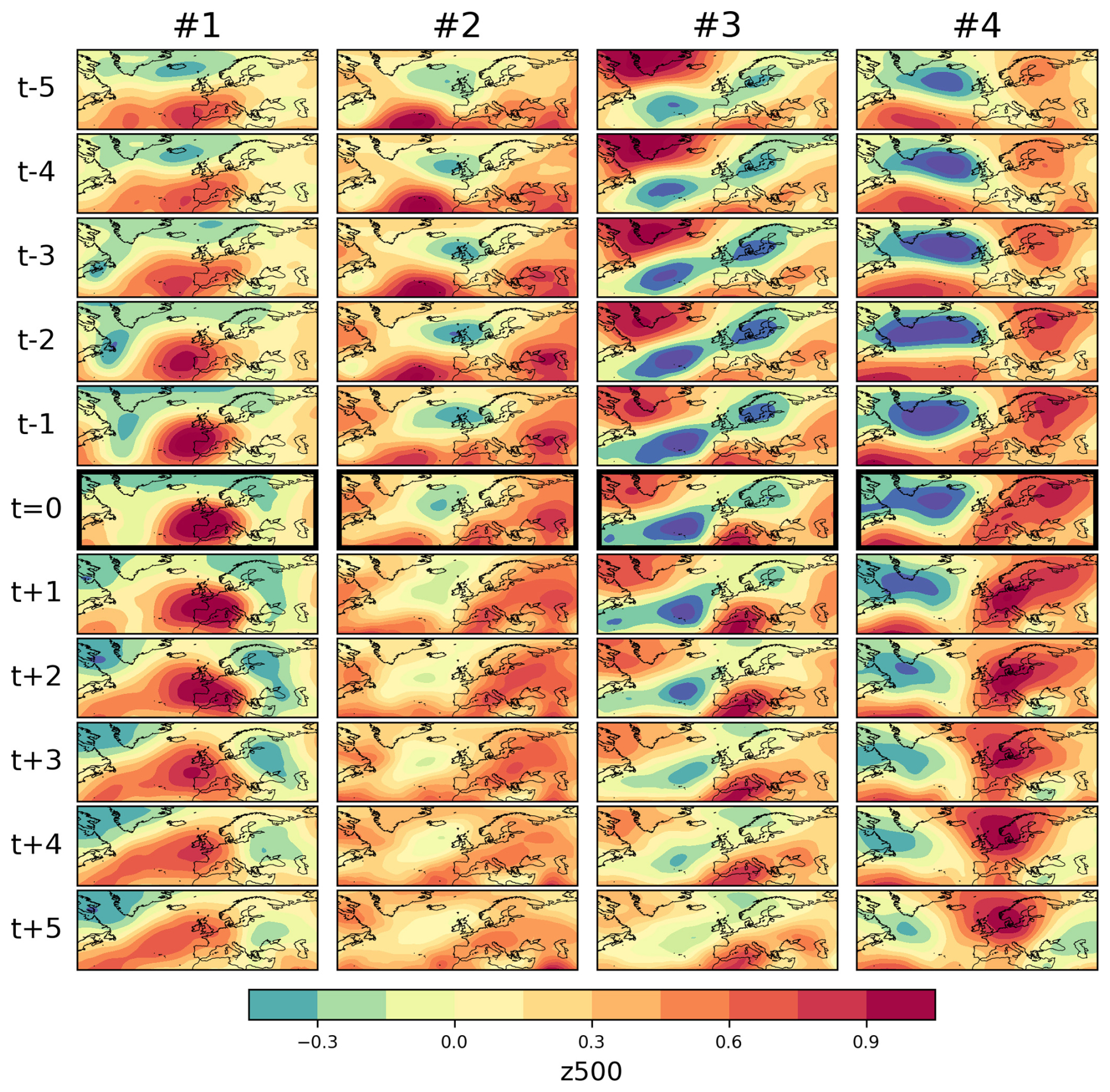
Figure A6 50-sample composite map.

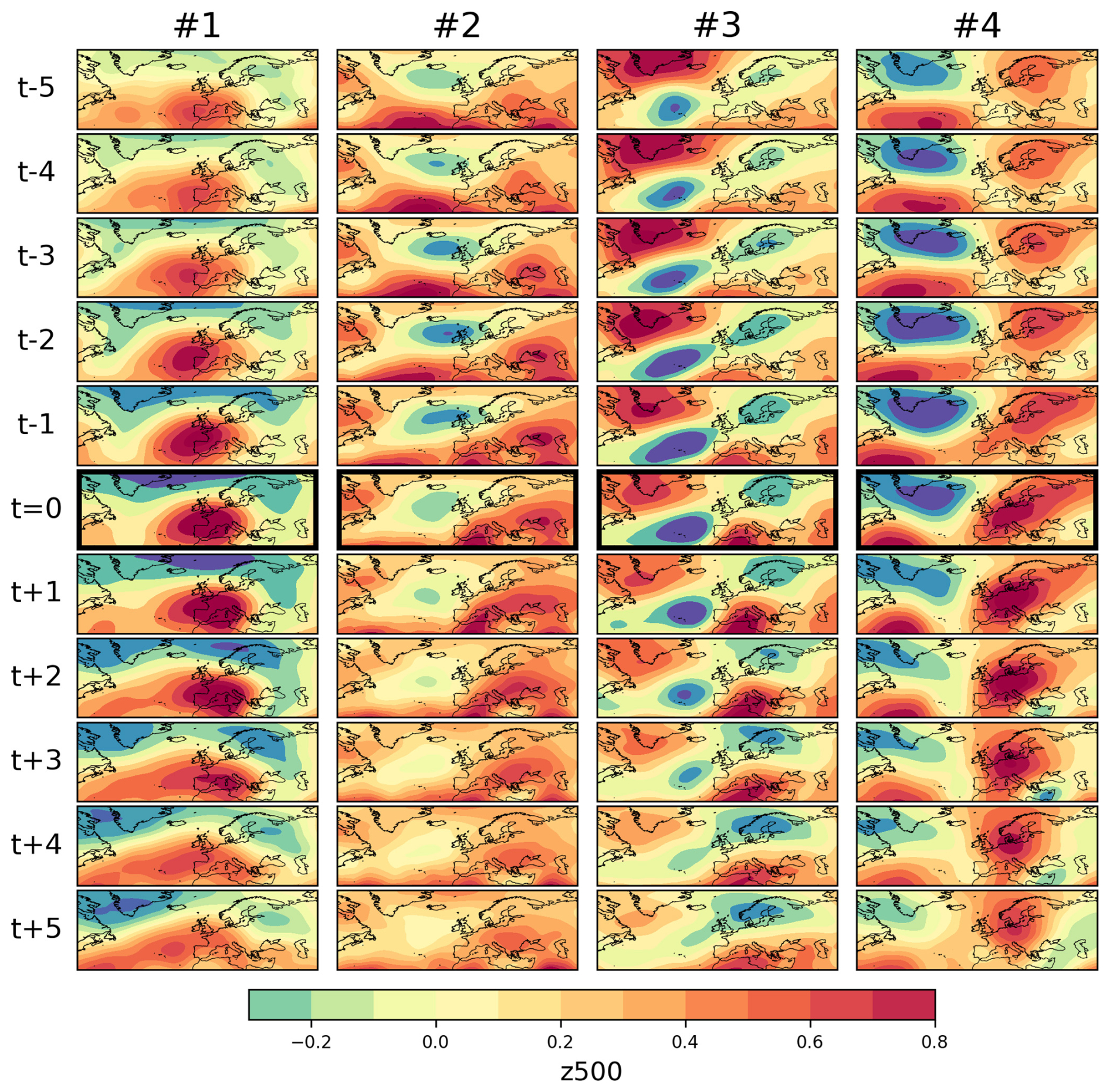
Figure A7 100-sample composite map.

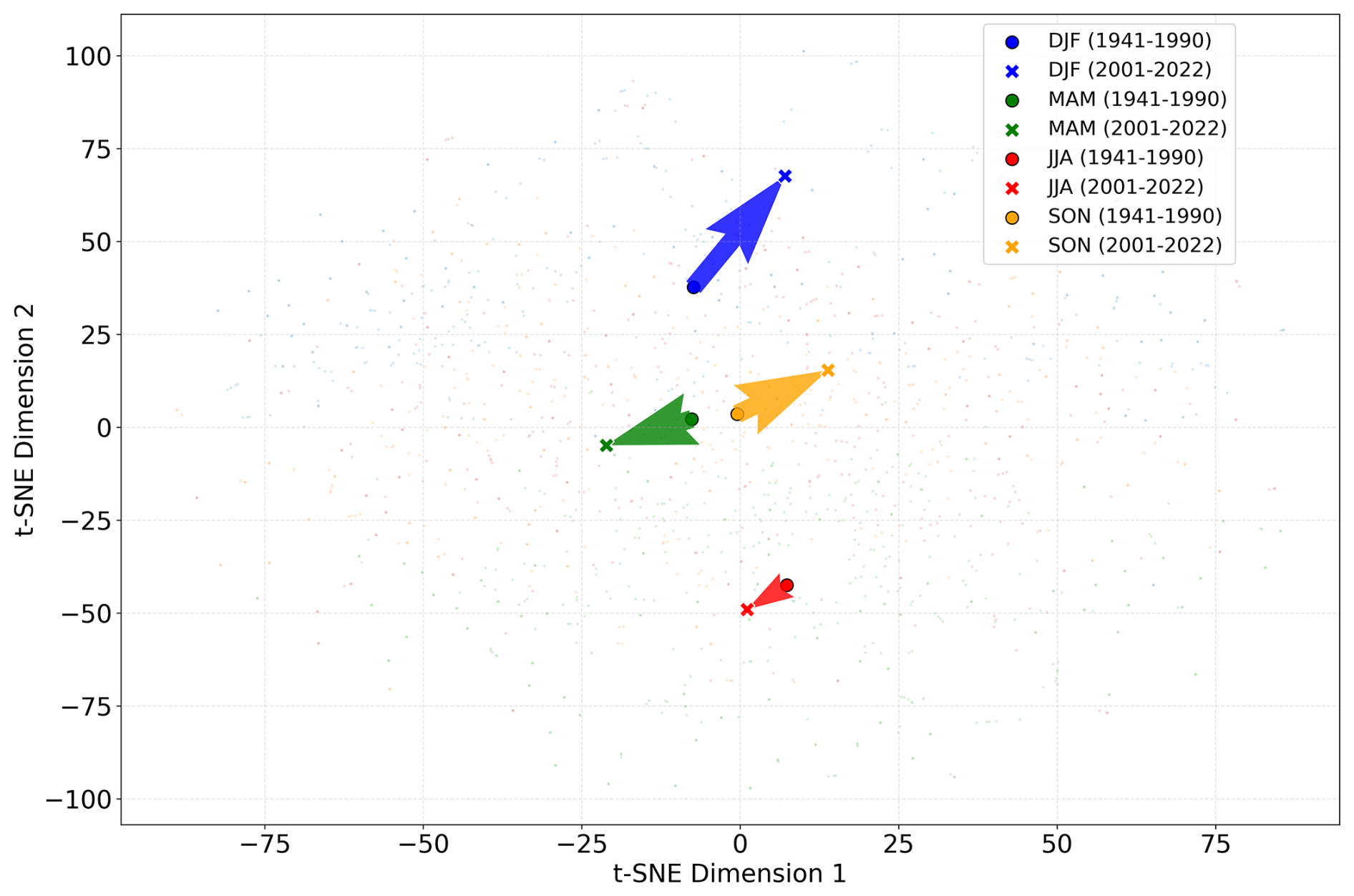
Figure A8 Temporal evolution of seasonal atmospheric patterns in the VAE latent space using detrended data. Vectors indicate the shift in mean latent embeddings for heatwave samples between 1941–1990 and 2001–2022 for Winter (blue), Spring (green), Summer (red), and Autumn (orange). All shifts are statistically significant (p<0.001). Winter patterns exhibit the most substantial displacement (Mahalanobis distance D=1.40)

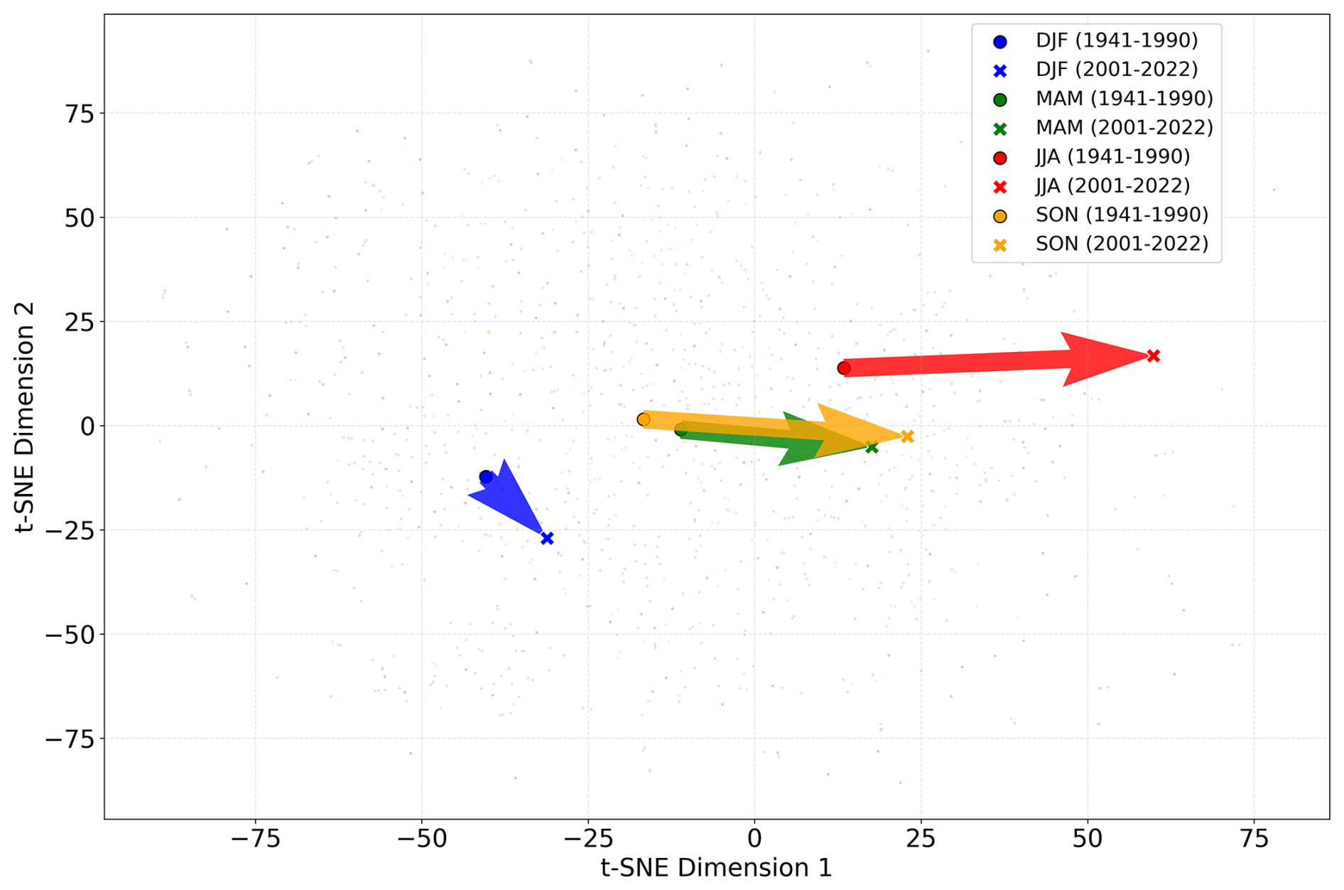
Figure A9 Temporal evolution of seasonal atmospheric patterns in the VAE latent space using non-detrended data. Vectors show the distributional drift between train (1941–1990) and test (2001–2022) periods. In this dataset, summer patterns show the largest shift (D=2.00), dominated by thermodynamic warming, which contributes approximately 83 % of the signal. This highlights that summer heatwave evolution is primarily driven by thermodynamic factors (p<0.001).

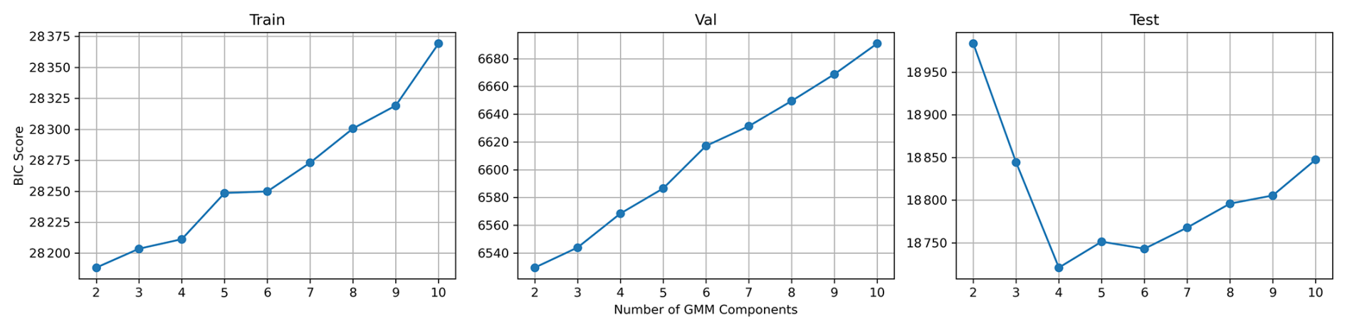
Figure A10 Bayesian Information Criterion (BIC) scores for GMM clustering across 2–10 components. Each panel shows the BIC scores for a different dataset split: (left) training period (1941–1990), (middle) validation period (1991–2000), and (right) testing period (2001–2022). The test set shows a clear minimum BIC score at four components, suggesting this is the optimal number of clusters under the BIC criterion. In contrast, the training and validation sets exhibit steadily increasing BIC scores as components are added, favoring simpler models. Despite these differences, the four-component model provides a balance between underfitting and overfitting across all periods.

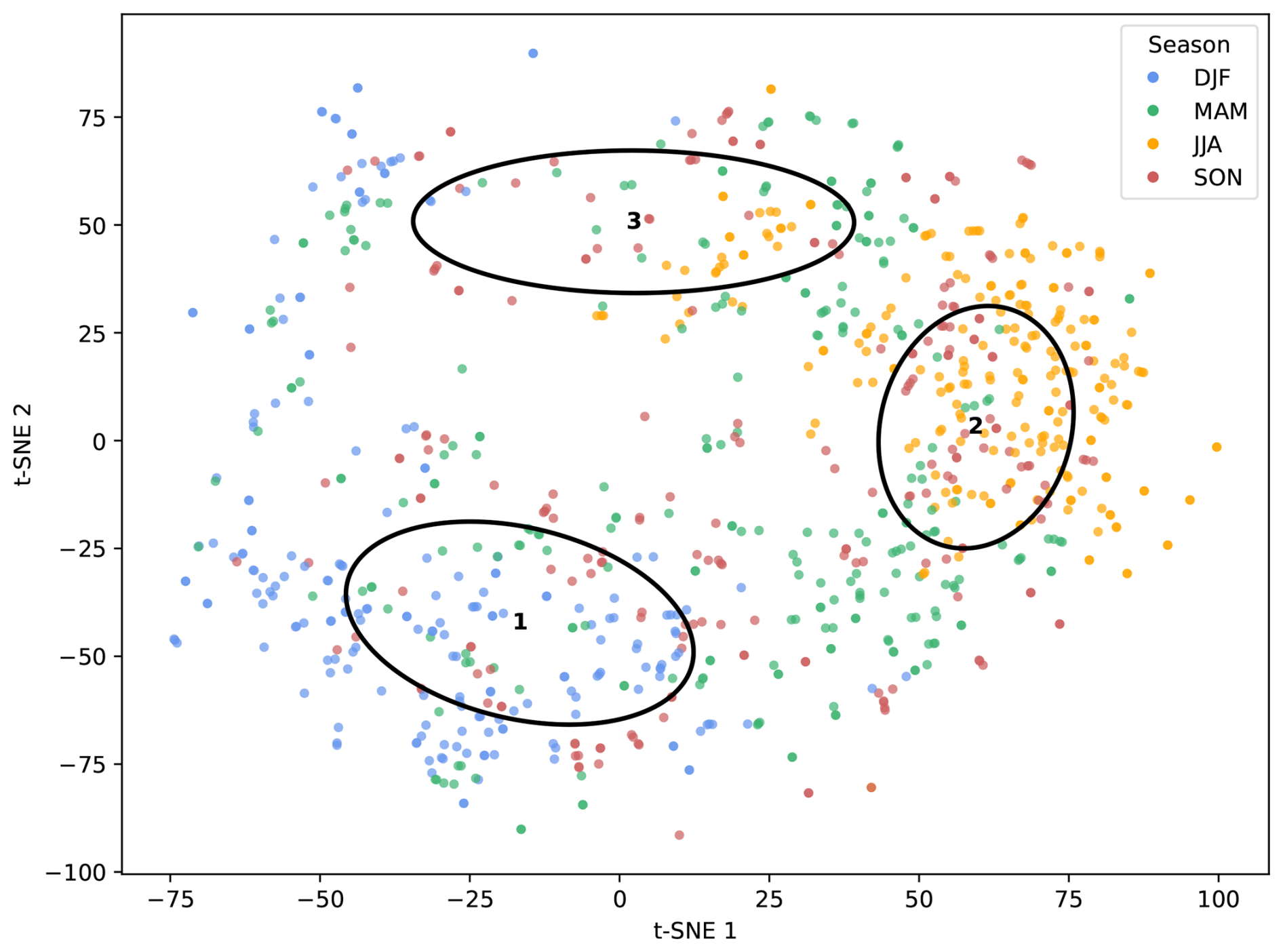
Figure A11 t-SNE representation of the latent space with three corresponding GMM components. Each point represents a heatwave sample. Colors represent the seasons in which the sample onset dates are located.

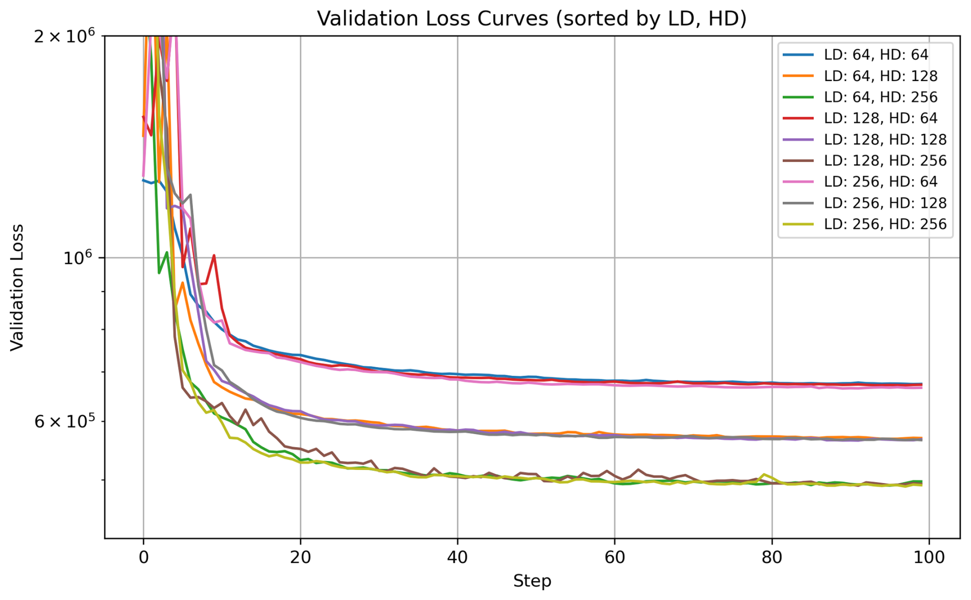
Figure A12 Validation loss curves for combinations of latent dimension (LD) and hidden dimension (HD). Each line shows the validation loss over training steps for a specific pair of LD and HD values. Higher-dimensional representations substantially improve reconstruction accuracy.

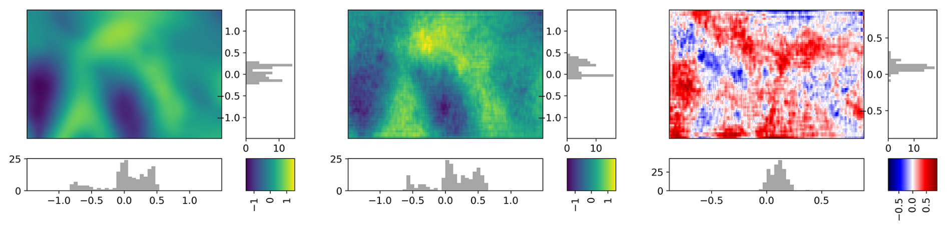
Figure A13 Geopotential height at 500 hPa for a random sample (left), its VAE reconstruction (middle), and the resulting reconstruction bias (right), each averaged over the time dimension. The histograms below each panel show the distributions of longitudinal and latitudinal values, respectively.

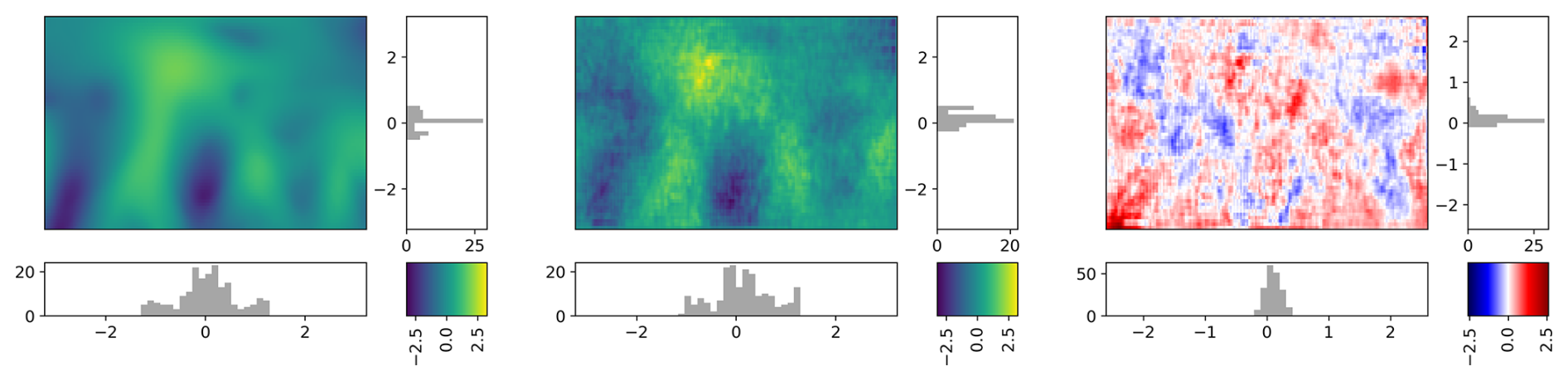
Figure A14 Geopotential height at 500 hPa for a random sample (left), its VAE reconstruction (middle), and the resulting reconstruction bias (right), each shown at the onset date. The histograms below each panel show the distributions of longitudinal and latitudinal values, respectively.

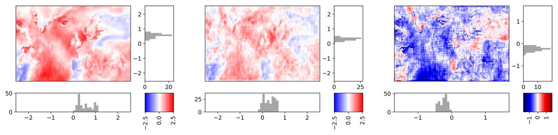
Figure A15 2 m temperature for a random sample (left), its VAE reconstruction (middle), and the resulting reconstruction bias (right), each averaged over the time dimension. The histograms below each panel show the distributions of longitudinal and latitudinal values, respectively.

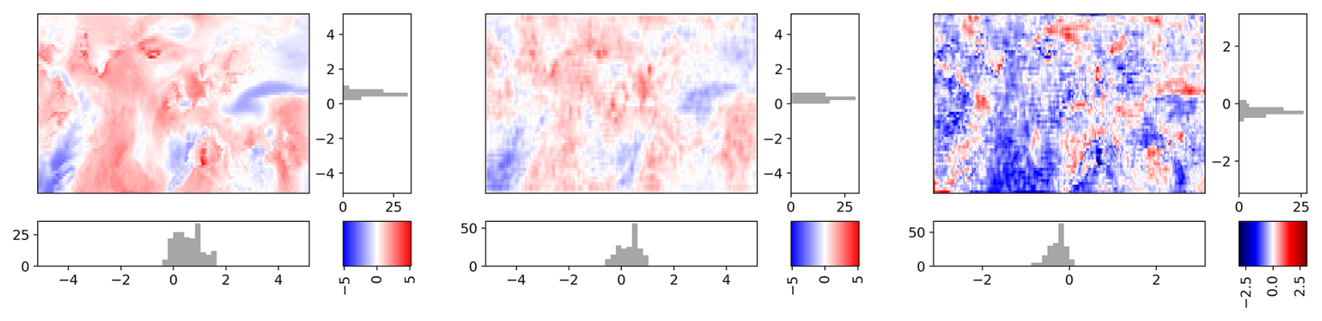
Figure A16 2 m temperature for a random sample (left), its VAE reconstruction (middle), and the resulting reconstruction bias (right), each shown at the onset date. The histograms below each panel show the distributions of longitudinal and latitudinal values, respectively.