Deep learning-based chlorophyll prediction: comparison with a dynamic model and applications to fish catch forecasting

Anticipating marine ecosystem changes is critical for enabling communities to adapt to climate fluctuations and for predicting future climate by considering interactions between Earth's physical and biogeochemical fields. Earth System Models (ESMs) capture large-scale physical–biogeochemical coupling, but their biogeochemical prediction skill varies substantially across regions and lead times due to sparse observational records, structural uncertainties in biogeochemical models. Here, we develop a deep learning-based prediction system to forecast surface chlorophyll concentrations across all Large Marine Ecosystems (LMEs) at monthly to annual timescales with lead times up to two years. Trained on multi-decadal simulations from various climate models and a coupled physical–biogeochemical reanalysis from a data assimilative ESM run, the system demonstrates skillful chlorophyll predictions comparable to ESM-based dynamic forecasts. The prediction skill is associated with physical-biogeochemical coupling processes triggered by large-scale climate variability, consistent with the mechanisms previously identified in dynamical forecasts. Furthermore, predicted chlorophyll anomalies are significantly linked to interannual variability in fish catch in several LMEs, demonstrating the promise of data-driven biogeochemical forecasting to support adaptive, climate-informed marine resource management.

1 Introduction

Marine ecosystems play a pivotal role in regulating Earth's climate system, particularly through the cycling of carbon and other greenhouse gases at the ocean–atmosphere boundary (Volk and Hoffert, 1985; Falkowski et al., 2000). Phytoplankton, a central component of the marine ecosystem, drives the biological carbon pump via photosynthesis (Falkowski et al., 1998; Field et al., 1998) and also modulates the physical properties of the ocean surface, such as surface albedo and the vertical distribution of solar shortwave radiation, thereby influencing upper ocean temperature (Sweeney et al., 2005; Park et al., 2018a). These biogeochemical and biogeophysical feedbacks can affect large-scale climate variability and long-term global warming patterns across multiple timescales. Understanding and predicting marine biogeochemical variability is therefore critical for advancing climate predictions based on bio-climate interactions and supporting the sustainable management of marine ecosystems (Bonan and Doney, 2018; Siegel et al., 2023). This is particularly important for Large Marine Ecosystems (LMEs), productive coastal regions that account for the majority of the world's marine fish catch, and anticipating environmental changes in these regions is directly relevant to climate-informed fisheries management (Tommasi et al., 2017; Capotondi et al., 2019).

Translating this understanding into actionable biogeochemical prediction remains challenging. While Earth System Models (ESMs), which integrate biogeochemical processes within physical climate frameworks (Flato, 2011; Bonan and Doney, 2018), have demonstrated skillful forecasts of oceanic physical variables on seasonal to decadal timescales (Smith et al., 2019; Balmaseda et al., 2024), recent advances have further shown prediction skill for biogeochemical variables including net primary production (Krumhardt et al., 2020), ocean carbon fluxes (Ilyina et al., 2021), ocean acidification (Brady et al., 2020), ecosystem stressors (Mogen et al., 2023), and seasonal to multiannual chlorophyll fluctuations across several regions (Park et al., 2019). Yet prediction skill varies substantially across LMEs and lead times. ESM-based biogeochemical forecasting remains constrained by limited observational records for biogeochemical fields, with satellite-derived chlorophyll a records extending only since the late 1990 s (Henson et al., 2010; Henson et al., 2016), structural uncertainties in biogeochemical models (Séférian et al., 2020; Fennel et al., 2022), large inter-model discrepancies, particularly where observational constraints are insufficient (Mignot et al., 2023; Kwiatkowski et al., 2020), and the substantial computational costs required for ensemble experiments (Balaji et al., 2022). These constraints have highlighted the need for alternative methodologies that can provide skillful biogeochemical forecasts at the scale of LMEs with greater computational efficiency.

Deep learning has emerged as a promising alternative for predicting marine biogeochemical variability. These data-driven models can learn complex, nonlinear relationships and can be trained on data-rich climate model simulations to overcome the limited length of observational records and structural uncertainties in process-based models, making them well-suited for seasonal-to-annual biogeochemical forecasting (Reichstein et al., 2019). Having demonstrated skills in forecasting physical ocean variables and major climate modes including El Niño–Southern Oscillation (ENSO) and the Indian Ocean Dipole (IOD) across various timescales (Biswas and Sinha, 2021; Xiao et al., 2019; Song et al., 2020; Immas et al., 2021; Ham et al., 2019), deep learning has more recently been applied to biogeochemical domains, including historical chlorophyll a reconstruction (Roussillon et al., 2023), phytoplankton biomass estimation (Yu et al., 2020), satellite data gap-filling (Hong et al., 2023), and biogeochemical forecasting applications in regional marine systems (Cen et al., 2022; Yao et al., 2023). Despite this progress, existing efforts often lack global spatial scope, suffer from limited interpretability due to their “black box” nature, and show limited connection to underlying physical–biogeochemical mechanisms.

To address these limitations, we developed a global-scale forecasting framework based on a convolutional neural network (CNN) to predict surface chlorophyll anomalies across all LMEs (Fig. 1). While complementary efforts have explored hybrid approaches that embed AI corrections within process-based models (Banerjee et al., 2026), our framework takes a purely data-driven approach, ingesting three consecutive months of global sea surface temperature and chlorophyll anomalies to produce monthly or annual chlorophyll forecasts at the LME scale with lead times of 1–24 months, aligning with the temporal scales relevant for marine resource management decisions including seasonal quota setting, harvest control adjustments, and interannual stock assessment planning (Stock et al., 2015; Tommasi et al., 2017). The model is trained on multi-decadal climate model simulations from the Coupled Model Intercomparison Project phase 6 (CMIP6) (Eyring et al., 2016) and physical–biogeochemical reanalysis data (Park et al., 2018b), allowing it to learn from a broader range of climate variability than the satellite record alone provides. Model predictions are evaluated against satellite-derived chlorophyll, and compared with ESM-based dynamical biogeochemical forecasts. Sensitivity experiments and interpretability analysis further connect the model's predictions to underlying physical–biogeochemical drivers (details in Sect. 2).

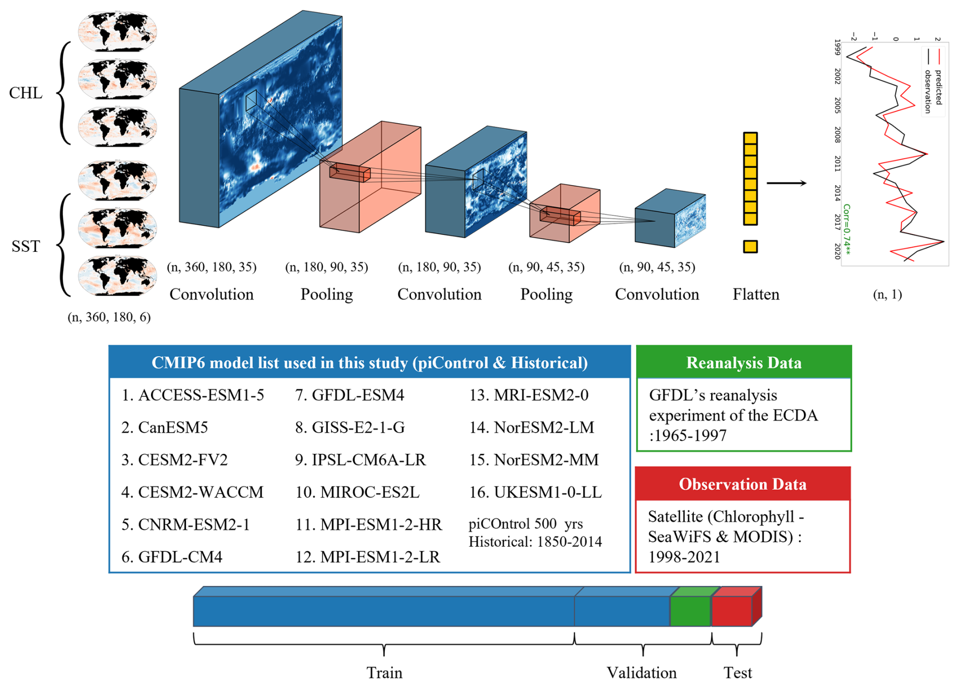
Figure 1 Deep learning model structure. The adapted CNN model comprises three convolutional layers (blue), two max-pooling (MP) layers (red), and one fully connected (FC) layer (yellow). Input data include sea surface temperature (SST) and chlorophyll anomalies for three consecutive months (e.g., November–January), represented as six channels. The model predicts either monthly or annual mean chlorophyll anomalies for each Large Marine Ecosystem (LME). Training data comprise historical and piControl simulations from 16 CMIP6 models, along with physical–biogeochemical reanalysis (1965–1997). Model validation was performed using satellite-based chlorophyll observations from SeaWiFS and MODIS (1998–2021).

2 Methods

2.1 Deep learning model and forecast experiment design

The CNN model used in this study was adapted from prior work on spatiotemporal prediction (Ham et al., 2019). It consists of an input layer followed by three convolutional layers, two max-pooling layers, one fully connected layer, and an output layer. The network incorporates 35 convolutional filters per layer, uses Gaussian Error Linear Unit (GELU) activation functions (Hendrycks and Gimpel, 2016), and is trained using the Mean Absolute Error (MAE) loss function. These configuration choices were identified through systematic sensitivity analysis (Sect. 3.1). The complete hyperparameter specifications are provided in Table S1 in the Supplement.

The model predicts area-averaged chlorophyll anomalies for individual LMEs from global spatial fields. Input data consist of three consecutive monthly global maps of SST and chlorophyll anomalies, gridded at 1°×1° resolution (360 longitude×180 latitude) and represented as six input channels. The model output is a single scalar value representing the LME-averaged chlorophyll anomaly at the target lead time. Separate CNN models sharing the same architecture are trained for each combination of target LME, forecast type (annual or monthly mean), and lead time.

For annual forecasts, the input window is fixed to boreal winter (November–December–January), and models predict the annual mean chlorophyll anomaly for the target LME in the year following the forecast start. For monthly forecasts, CNN models cover all combinations of forecast start months and lead times (1–24 months ahead), each predicting the chlorophyll anomaly for a specific target month. Lead time is defined as the number of months between the final month of the input window and the target month. For example, using inputs from October, November, and December (OND) to predict the January chlorophyll anomaly corresponds to a 1 month lead time. This enables evaluation of how predictability varies with forecast timing and horizon (Sect. 3.2). Chlorophyll anomalies are defined as deviations from monthly climatological means, computed separately for each dataset (CMIP6 models, reanalysis, satellite observations) over their respective reference periods. Prediction performance was evaluated using the anomaly correlation coefficient (ACC), computed as the temporal correlation between predicted and observed time series of LME-averaged chlorophyll anomalies. Statistical significance was assessed following a method using effective degrees of freedom corrected for temporal autocorrelation (Bretherton et al., 1999):

$$\begin{array}{}\text{(1)}& N_{\text{eff}}={\displaystyle \frac{N}{{\sum }_{t=\mathrm{0}}^{t=N-\mathrm{1}}\left(\mathrm{1}-\frac{t}{N}\right)r_t^{\mathrm{F}}{r}_t^{\mathrm{O}}}},\end{array}$$

where N is the number of samples in the forecast (F) and observed (O) time series, and $r_t^{\mathrm{F}}$ and $r_t^{\mathrm{O}}$ are estimates of autocorrelation in each time series at lag t.

2.2 Data sources and preprocessing

This section describes the data sources used for training, validation, and testing, with sample sizes and temporal coverage detailed in Table S2 in the Supplement. The model was trained on CMIP6 historical and preindustrial control simulations (16 models) combined with GFDL-ECDA reanalysis (Park et al., 2018b), totalling 8013 samples. A subset of CMIP6 simulations and reanalysis data (2043 samples) was held out for validation during training to monitor convergence and prevent overfitting. For sensitivity experiments (Sect. 3.1), model performance was evaluated on GFDL-ECDA reanalysis (1998–2017), independent from the training period. Final model evaluation used satellite-derived chlorophyll from SeaWiFS and MODIS (1998–2021), fully independent from all model development data. Where ensemble predictions were required, 5-member ensembles were generated by training five models with identical architecture and data but different random weight initializations.

Long-term simulated chlorophyll and SST data were drawn from historical and preindustrial control (piControl) runs of 16 models from the Coupled Model Intercomparison Project Phase 6 (CMIP6). Historical simulations, driven by observed time-varying external forcings over 1850–2014, and piControl simulations, run under fixed pre-industrial forcing to provide multi-century records of internal climate variability, were used for training. Given variability in the length of piControl simulations among models, only the most recent 500 years were used when available; for models with shorter records, the entire simulation period was included. CMIP6 simulations were employed exclusively for training and validation purposes.

Reanalysis data used for validation and sensitivity testing were obtained from the NOAA Geophysical Fluid Dynamics Laboratory's Ensemble Coupled Data Assimilation (GFDL-ECDA) system, integrated with the COBALT biogeochemical model (Park et al., 2018b). This system assimilates observed physical variables into a coupled physical–biogeochemical framework while excluding direct assimilation of biogeochemical variables to avoid spurious vertical velocity artifacts near the equator. Data from 1965–1997 were used for validation, while the 1998–2017 period supported sensitivity analysis.

Satellite monthly surface chlorophyll a concentrations were obtained from the SeaWiFS and MODIS ocean color sensors (Esaias et al., 1998; Mcclain, 1998), and sea surface temperature (SST) data were from NOAA's optimally interpolated SST version 2 (OISSTv2) dataset based on the Advanced Very High Resolution Radiometer (AVHRR) (Reynolds et al., 2007). The original chlorophyll and SST data were provided at monthly resolution with fine spatial scales (0.25° for SST and 9 km×9 km for chlorophyll). For consistency and computational efficiency in deep learning applications, all observational data spanning 1998–2021 were interpolated onto a 1°×1° regular global grid. Following standard practice (Campbell, 1995), the median value within each grid cell was used during spatial interpolation of chlorophyll to account for the lognormal distribution of chlorophyll concentration.

Due to cloud cover and persistent polar night, the ocean color datasets contained spatially and temporally varying missing values. To ensure spatial consistency across all datasets, we constructed a unified binary mask from the satellite record: any grid cell containing a missing value in any single month during the entire satellite period (1998–2021) was permanently flagged. All flagged grid cells were set to zero across all time steps. The mask itself was not provided as an explicit input channel to the model. The consistently zero-valued regions largely correspond to land-adjacent, polar, or persistently cloud-covered areas where chlorophyll signals are typically absent or negligible, reducing the likelihood that zero-filling introduces spurious learning signals. Land grid cells are also represented as zero in the input fields. Because both land and masked ocean grid cells maintain constant zero values across all time steps and all training samples, they carry no temporal variability and thus contribute no learnable signal to the CNN. The network effectively learns to rely on grid cells with non-zero, time-varying inputs. SST fields were not subject to this masking, as the optimally interpolated SST product provides near-complete global coverage. The same unified mask derived from satellite observations was applied to simulated chlorophyll fields, with masked grid cells set to zero, ensuring that the spatial domain used for training is identical to that used for evaluation.

2.3 SHAP Analysis

To interpret the model's predictions and identify dominant spatial drivers, we applied SHapley Additive exPlanations (SHAP) (Lundberg et al., 2020, 2018). SHAP provides feature-level attributions by estimating the marginal contribution of each input (grid cell) to the final model output. For each prediction, the SHAP decomposition follows Eq. (2):

$$\begin{array}{}\text{(2)}& y=\stackrel{\mathrm{‾}}{y}+\sum _i{\mathit{\phi }}_i,\end{array}$$

where y is the prediction, $\stackrel{\mathrm{‾}}{y}$ is the mean prediction, and φ_i is the SHAP value (i.e., the contribution) of feature i, which in this case corresponds to a specific grid point in the input map. Each feature corresponds to a specific grid point in one of six input channels: three consecutive months of chlorophyll anomalies and three consecutive months of SST anomalies. We compute SHAP values separately for SST and chlorophyll by aggregating across their respective three monthly channels, then visualize them as spatial attribution maps. These maps reveal which area of the input fields most strongly influence the predicted chlorophyll anomaly in each target LME at different forecast lead times. Additionally, comparing the spatial extent and magnitude of SHAP values between SST and chlorophyll maps allows us to assess the relative importance of physical versus biological drivers for each region's predictability.

Because the target variable is chlorophyll concentration anomalies, which can be positive or negative, we analyze the absolute SHAP values to interpret how each grid point contributes to pushing the anomalies in either the positive or negative direction. Large absolute SHAP values indicate that the input conditions at a particular grid point have a strong influence on the predicted chlorophyll anomaly for the region of interest. SHAP values are calculated by estimating the marginal contribution of each grid point across all possible permutations of the input map. This is done by comparing the model's predictions with and without the grid point of interest, while considering all possible subsets of the other grid points. The 'absence' of a grid point is simulated not by zero substitution, but by averaging the model's predictions over a range of plausible values for that location, drawn from the input data distribution.

2.4 Comparison with the dynamical forecast system

The dynamical system, developed at the Geophysical Fluid Dynamics Laboratory (GFDL), builds on a seasonal climate prediction framework with a coupled ocean–atmosphere data assimilation system and is run with a marine ecosystem model, the Carbon, Ocean Biogeochemistry and Lower Tropics (COBALT) (Zhang et al., 2007; Stock et al., 2014). The retrospective predictions were initialized on the first day of each calendar month from 1991–2017 and consist of 2-year-long forecasts with 12-member ensembles (see Park et al., 2019, for details).

To compare the prediction skill of the deep learning and dynamic models, we employed a double bootstrap procedure that accounts for two independent sources of uncertainty in the deep learning model: ensemble variability and temporal sampling variability. For each LME, we performed 1000 bootstrap iterations. In each iteration, we first resampled five ensemble members with replacement from the five independently trained CNN members (each initialized with different random weights) and computed their ensemble mean prediction. We then subsampled 20 years without replacement from the full 24 year test period (1998–2021) to match the verification period length of the dynamic model (1998–2017). The Pearson correlation coefficient between the resampled ensemble mean predictions and satellite observations was computed over the subsampled years, yielding a bootstrap distribution of deep learning correlation skill for each LME. From this distribution, we derived the 95 % confidence interval (2.5th–97.5th percentile) and a one-sided bootstrap p-value, defined as the fraction of bootstrap samples where the deep learning correlation is equal to or less than the dynamic model's correlation.

For spatial comparison, LMEs were classified based on the following criteria. Each model's skill was first assessed for statistical significance (positive correlation with p<0.10), using effective degrees of freedom to account for temporal autocorrelation (Bretherton et al., 1999). If only one model showed significant skill, that model was assigned as superior. When both models showed significant skill, the bootstrap p-value determined the classification: DL superior (p<0.05), dynamic model superior (p>0.95), or no significant difference ($\mathrm{0.05}\le p\le \mathrm{0.95}$). LMEs where neither model achieved significant skill, or where data were unavailable, were classified as not comparable. The bootstrap procedure was applied only to the deep learning model because raw prediction fields from the dynamic model were not available; only pre-computed correlation values were accessible.

2.5 Fisheries data and skill assessment for fish catch prediction

We utilized annual reported fish catch data from the Sea Around Us project (Pauly and Zeller, 2016), which compiles species-resolved annual harvests by LME. Total annual catches per species were calculated, and ambiguous or non-specific entries were excluded. Only LMEs in which the CNN demonstrated significant chlorophyll prediction skill were considered, as skillful prediction is a prerequisite for chlorophyll to serve as a predictable bottom-up driver of fisheries variability. While fish catch is influenced by numerous factors, including fishing effort, management policies, and physical oceanographic conditions, chlorophyll represents one potential bottom-up forcing pathway linking environmental variability to marine resource fluctuations.

For each selected LME, the ten most harvested species were identified by cumulative catch volume. Catch anomalies were computed as normalized values by subtracting the mean and dividing by the standard deviation for each species. Simple linear regression was applied to predict normalized fish catch anomalies using annual chlorophyll anomaly forecasts generated by providing the CNN with satellite observations from NDJ (November of Year 0–January of Year 1), at lag=0 (same year) and lag=1 (following year). Results were back-transformed to the original units (tonnes) for presentation. Species–LME combinations were retained where statistically significant correlations were identified, and supporting ecological literature suggested a plausible bottom-up forcing mechanism. Statistical significance of correlation coefficients between predicted and reported fish catch was assessed using effective degrees of freedom to account for temporal autocorrelation (Bretherton et al., 1999), similar to the statistical test for chlorophyll prediction, and evaluated at p<0.05 and p<0.10 levels. The regression was fitted over the entire analysis period. This analysis is intended as an exploratory demonstration of potential downstream applications of the chlorophyll forecasting framework, rather than a validated fisheries prediction system.

3 Results

3.1 Sensitivity experiments of model configuration

A systematic evaluation of model configurations was performed to assess how architectural and data choices affect chlorophyll prediction skill across global marine ecosystems (Fig. 2). For computational efficiency, the sensitivity experiments were conducted on 16 representative LMEs (Fig. S1 in the Supplement). Prediction skill was quantified as the anomaly correlation coefficient (ACC) between predicted and GFDL-ECDA reanalysis annual chlorophyll anomalies (1998–2017), averaged across these regions for comparison. Starting from a baseline configuration with commonly used settings (ReLU activation functions and mean squared error loss), we systematically evaluated modifications to individual components, including activation functions and loss functions (MAE), kernel sizes, and data composition (Table 1). This allowed us to identify the most robust and efficient combination, which was then adopted as our reference model. To streamline the presentation in Fig. 2, the sensitivity results are organized around this reference. Each blue bar represents a variant differing by only a single component, providing a direct visualization of how individual choices influence predictive skill.

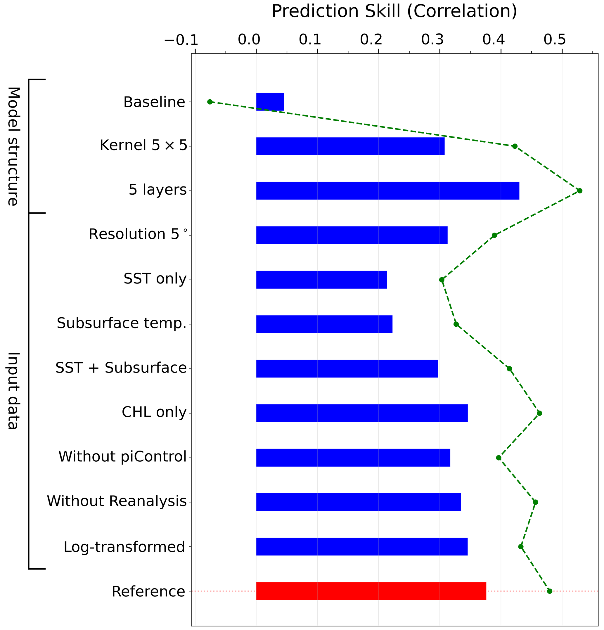
Figure 2 Sensitivity test of model configuration. Bars indicate the average correlation skill across 16 selected regions for each model variation. The reference model (red bar), was identified through this sensitivity analysis as the configuration with the best balance of predictive skill, spatial robustness, and computational efficiency. In each sensitivity experiment (blue bars), a single component differs from the reference configuration, either a structural aspect (e.g., kernel size, number of layers) or input data configuration (e.g., resolution, predictor variables, log transformation). The baseline model, shown at the top, shares the same architecture as the reference model but uses standard training settings (ReLU activation, MSE loss). The green dashed line shows the average skill across regions where prediction was statistically significant (p<0.10) in at least one configuration. See Table 1 for detailed input variable configurations corresponding to each experiment shown.

Table 1 Sensitivity experiment configurations. Each experiment modifies one component relative to the reference model (bottom row), with all other settings held constant. Sig. LMEs indicate the number of regions with statistically significant prediction skill (p<0.10) out of 16 representative LMEs. Training: CMIP6 historical (1850–2014) + piControl (500 years) + GFDL-ECDA reanalysis (1965–1997). Validation: GFDL-ECDA reanalysis (1998–2017). Abbreviations: CHL – surface chlorophyll anomalies; θ – subsurface potential temperature (0–300 m average); hist – historical; piC – piControl. “–” in the Architecture column indicates the same configuration as the reference model (3×3 kernel, GELU, MAE). Note: Prediction skill measured as ACC averaged across 16 representative LMEs.

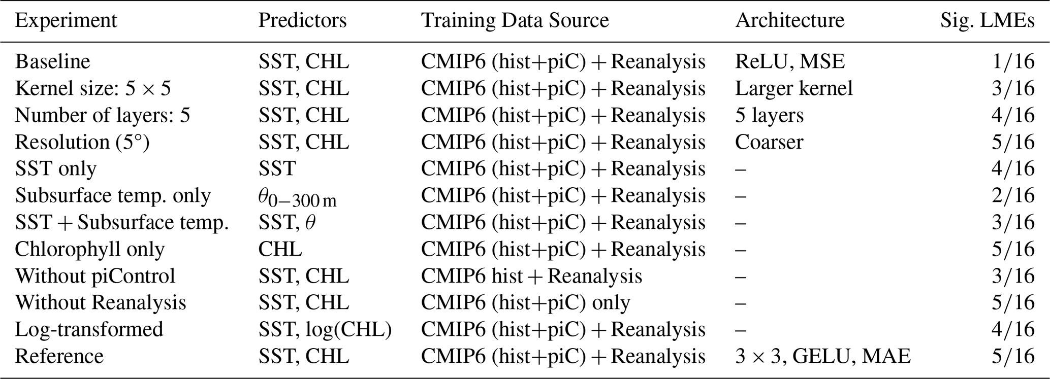
Regarding model architecture, replacing the 3×3 convolutional kernels in the reference model with broader 5×5 kernels reduced prediction skill despite the increase in trainable parameters, suggesting that the smaller kernel size is more effective at capturing local structure relevant to chlorophyll variability. Although increasing the network depth from 3–5 convolutional layers yielded a marginally higher mean ACC, the 3-layer reference achieved statistically significant skill in a larger number of LMEs (5 out of 16) than the 5-layer configuration (4 out of 16). Given that this study aims to identify regions where chlorophyll forecasts can be reliably generated, we prioritized the consistency of statistically significant skill across LMEs over a marginal gain in mean ACC. Combined with the substantial computational cost of training a 5-layer architecture across the large number of independent models required by our main analysis (12 forecast start months × 24 lead times for two representative LMEs in the monthly forecasts, and 66 LMEs in the annual forecasts, all as 5-member ensembles), the 3-layer configuration was adopted as the reference model.

In addition to architectural considerations, model performance was highly sensitive to input data configuration and preprocessing. High-resolution (1°) input data produced markedly higher predictive skill than coarser (5°) fields, reflecting the importance of resolving mesoscale variability that drives chlorophyll dynamics (Keerthi et al., 2022). Predictor selection for the input data proved equally critical: models trained with surface chlorophyll anomalies as input substantially outperformed those using only physical variables, such as sea surface temperature (SST) or subsurface potential temperature. Even combining SST with subsurface temperature did not match the skill achieved when chlorophyll was included as a predictor, underscoring the importance of biological initialization for chlorophyll forecasting. This improvement may reflect chlorophyll's temporal persistence, its sensitivity to subsurface conditions, or both. While chlorophyll alone showed substantial skill, combining it with SST yielded the highest performance, suggesting complementary predictive value (Park et al., 2018a).

The inclusion of additional training data sources improved the model's prediction skill. Incorporating CMIP6 piControl simulations, designed to represent long-term natural variability in the absence of anthropogenic forcing, enhanced the model performance by providing 500 years of diverse climate states beyond the limited satellite record. This enables the model to learn generalizable physical-biogeochemical relationships across a broader range of conditions. Similarly, inclusion of the ESM-based reanalysis product improved chlorophyll prediction skill by extending temporal coverage into the pre-satellite era with physically consistent, observationally constrained ocean states. This multi-source training approach helps mitigate overfitting to specific climate regimes while preserving physically meaningful patterns common across independent datasets.

Finally, the impact of applying a log transformation to chlorophyll data on the prediction skill was also tested. While log transformation is often used to normalize skewed chlorophyll distributions, our results indicate that retaining the original scale yields marginally higher average prediction skills. While the overall difference is modest, the untransformed input better preserves the dynamic range of chlorophyll variability in productive coastal LMEs, as log-scaling dampens high chlorophyll variability, which can lead to an underestimate in regions with high concentrations (Cen et al., 2022).

Overall findings here informed the development of an optimized model configuration that combines efficient model architecture, high-resolution inputs, ecologically meaningful predictors, and physically consistent long-term training data. Rather than representing ad hoc tuning, this configuration reflects deliberate design choices informed by empirical performance and domain knowledge. The reference model, which achieved the best overall balance of predictive skill and spatial robustness across the LMEs, serves as the foundation for all subsequent analyses, including model validation against satellite data, investigation of the mechanisms driving skillful predictions, and applications to fish catch forecasting.

3.2 LME-scale chlorophyll prediction

The reference model derived from the sensitivity experiments was applied across all global LMEs to evaluate its skill in forecasting monthly to annual chlorophyll anomalies. Annual forecasts were generated by providing the model with satellite observations of SST and chlorophyll from three consecutive months in early boreal winter (November–January), with the model predicting the following calendar year.

The model demonstrated skillful annual mean chlorophyll predictions in several LMEs (Fig. 3). These regions span across diverse oceanographic regimes, from the subarctic Eastern Bering Sea and a subtropical western boundary current (Agulhas) to semi-enclosed basins (Mediterranean, Gulf of California, East Sea), temperate shelf systems (Patagonian and Australian Shelves), and tropical-to-temperate coastal systems (Gulf of Mexico, U.S. Continental Shelves, Pacific Central-American Coastal) (Fig. 3b–n). The predicted chlorophyll anomalies successfully captured both interannual fluctuations and longer-term trends, closely following satellite-derived observations. Notably, many of these regions are known to exhibit chlorophyll variability linked to large-scale ocean-climate processes, a connection explored further in the following monthly-scale analysis.

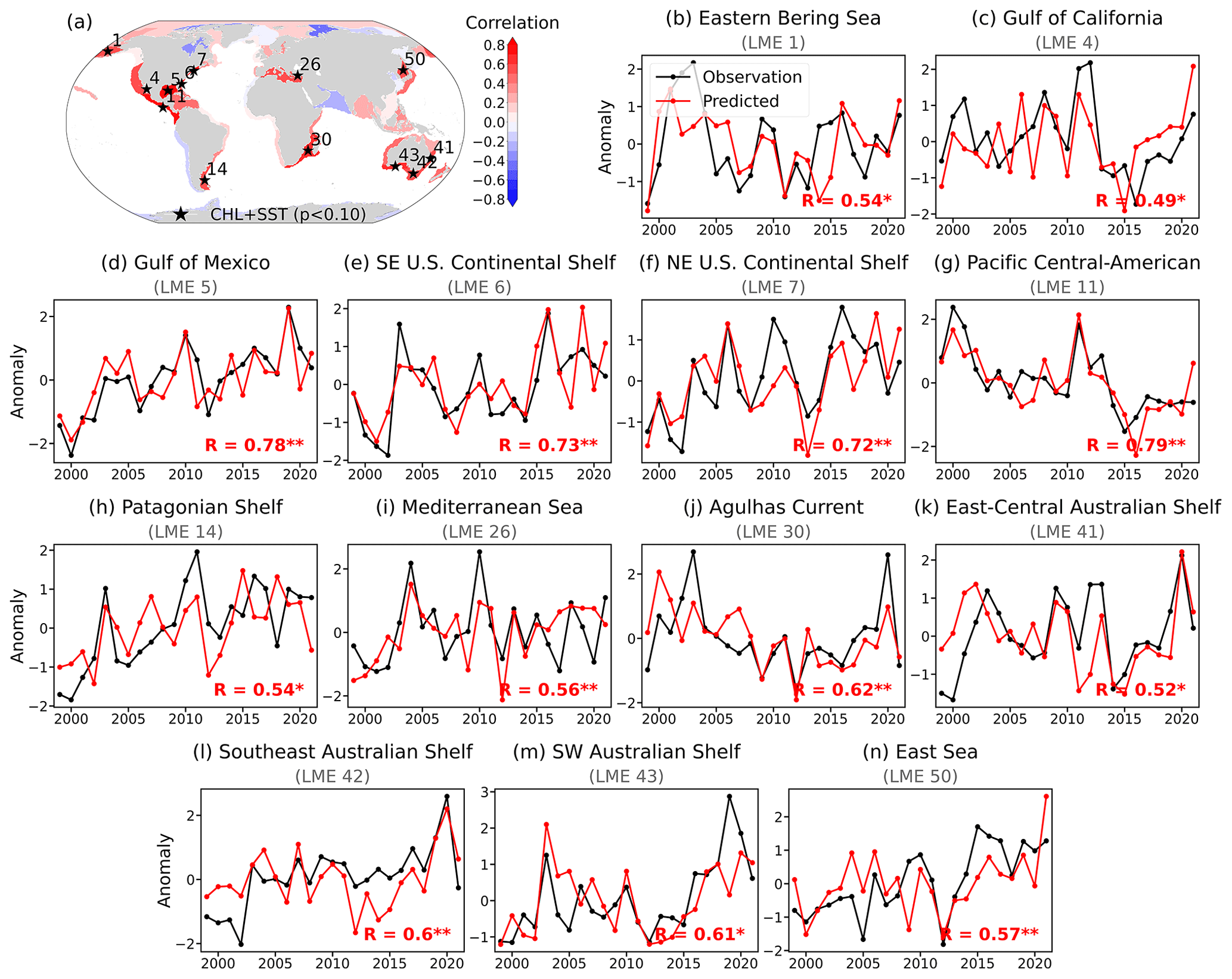
Figure 3 Chlorophyll prediction skill across Large Marine Ecosystems (LMEs). (a) Correlation coefficients between LME-averaged satellite-derived and predicted annual mean chlorophyll anomalies (1998–2021). The model takes November (Year 0)–December (Year 0)–January (Year 1) satellite observations as input and predicts the annual mean chlorophyll anomaly averaged over January–December of Year 1. Shading shows the prediction skill of the reference model using both chlorophyll (CHL) and sea surface temperature (SST) as input. Black asterisks mark LMEs with statistically significant correlations (p<0.1). (b–n) Time series of normalized annual mean chlorophyll anomalies from satellite observations (black) and model predictions (red) for the thirteen LMEs with significant prediction skill (corresponding to asterisks in panel a). Correlation values are indicated with significance levels (*: p<0.1, **: p<0.05).

To investigate the temporal structure of this predictability and the underlying mechanisms, chlorophyll prediction skill was further evaluated at monthly timescales. We examined monthly forecasts by selecting two representative systems from the Pacific and Indian Oceans, both exhibiting significant annual mean chlorophyll prediction skill and well-documented connections to large-scale climate variability in prior literature: the Pacific Central-American Coastal (LME 11) and the Agulhas Current (LME 30). For each LME, separate CNN models were trained for each combination of forecast start month and lead time (1–24 months), as described in Sect. 2.1. Model predictions were compared to satellite-derived chlorophyll anomalies after applying a 3 month moving average to facilitate skill assessment at seasonal scales.

In the Pacific Central-American region, the model exhibits seasonally varying forecast skill, with statistically significant correlations extending up to 12 month lead times for forecasts initialized during boreal winter (Fig. 4a). Prediction skill for chlorophyll is enhanced during boreal fall and winter, when large-scale climate variability such as ENSO is more predictable, but diminished during boreal spring and early summer, coinciding with the well-documented “spring predictability barrier” of ENSO. The model also consistently outperforms persistence forecasts across most initialization months at lead times up to approximately 12 months, with boreal winter initializations maintaining skill advantages at even longer leads (green circles in Fig. 4a). These patterns suggest that the model captures climate-driven signals to enhance chlorophyll prediction in this region, consistent with previous observational and modeling studies of primary productivity in the tropical Pacific (Park et al., 2019; Pennington et al., 2006; Sasai et al., 2012).

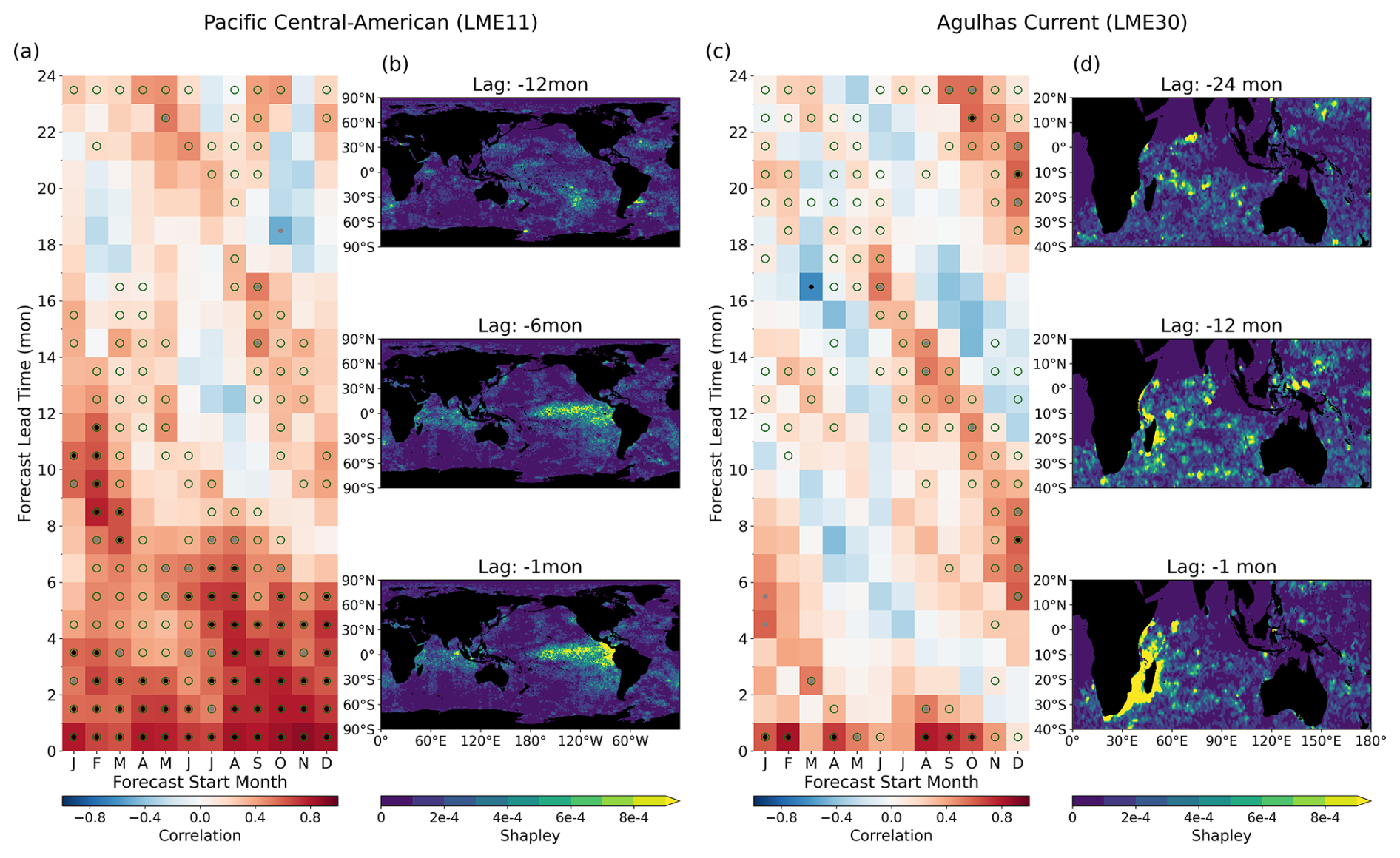
Figure 4 Monthly prediction and mechanism underlying chlorophyll prediction skill. (a, c) Anomaly correlation coefficient between predicted and satellite-observed monthly chlorophyll anomalies (LME-averaged) as a function of forecast start month (x-axis) and lead time (y-axis). Black dots indicate significant skill at p<0.05, while grey dots indicate p<0.10. Green open circles indicate skill exceeding the persistence model. (b, d) Spatial maps of absolute Shapley values at selected input lag times (indicated above each panel), illustrating which regions in the input fields contribute most to the predictions. Lag denotes the time offset of input observations relative to the forecast target period. For each LME, the Shapley values are shown for the most dominant predictor variable: SST for LME 11 (b; lags of −1, −6, and −12 months) and chlorophyll for LME 30 (d; lags of −1, −12, and −24 months).

In the Agulhas Current LME, the model exhibited a seasonally modulated pattern of forecast skill, marked by alternating bands of high and low correlation that persisted across lead times up to 24 months (Fig. 4c). This diagonal structure is particularly pronounced for austral winter initializations and resembles the winter-to-winter reemergence mechanism observed in dynamical prediction systems (Stock et al., 2015). In this process, wintertime anomalies are subducted beneath the mixed layer, preserved during summer stratification, and reemerge the following winter as seasonal mixing deepens the surface layer. The recurrence of this pattern in the model's predictions indicates that initial surface conditions reflect underlying subsurface ocean states, consistent with the demonstrated sensitivity of surface chlorophyll to subsurface dynamics (Park et al., 2018a; Lim et al., 2022; Lee et al., 2024).

3.3 Mechanisms underlying chlorophyll prediction skills

To examine the physical basis of the regional chlorophyll forecast skill, we applied SHAP to quantify the contribution of input features across lead times, focusing on the two regions where monthly forecasts were conducted. In the Pacific Central-American region, we examined boreal winter 2014–2015, which captured the early development phase of El Niño conditions, as documented by satellite chlorophyll observations. Attribution maps from the models initialized from this period reveal coherent patterns at 1-, 6-, and 12-month horizons, aligning with the canonical progression of ENSO-related anomalies, including the emergence and eastward propagation of SST signals along the equatorial Pacific (Fig. 4b). While SHAP does not infer causality, the spatial alignment between feature importance and known ENSO structures shows that the deep learning model can detect climate-scale variability relevant to chlorophyll prediction.

Attribution analysis during 2000–2002 in the Agulhas region, a period of peak chlorophyll concentrations in the region, revealed westward-propagating chlorophyll anomalies originating in the eastern Indian Ocean and extending toward the western boundary (Fig. 4d). This pattern is consistent with the dynamics of upwelling Rossby waves, which have been previously identified as key contributors to long-lead chlorophyll predictability in ESM-based dynamical forecasts in this region (Jeon et al., 2022). The presence of such physically interpretable propagation features indicates that the model captures spatiotemporal dynamics embedded in the training data, beyond surface-level statistical associations.

Results from both the Pacific Central-American Coastal and Agulhas Current LMEs demonstrate that the deep learning model captures physically interpretable signals underlying chlorophyll variability. The seasonally modulated skill patterns are consistent with the ENSO spring predictability barrier and wintertime reemergence of subsurface anomalies (Fig. 4a and c), while SHAP-based attribution identifies spatial features aligned with ENSO evolution and westward-propagating off-equatorial Rossby waves (Fig. 4b and d). Together, these findings suggest that the model internalizes aspects of coupled physical–biogeochemical dynamics from the training data, highlighting the potential of data-driven approaches to support mechanistically informed, climate-relevant biogeochemical forecasts.

3.4 Prediction skill comparison with dynamic forecasts

We next compared the predictive performance of our deep learning model with that of a dynamical prediction system to assess relative skill (see Sect. 2.4 for a description of the dynamical system). Chlorophyll prediction skill was evaluated against an ESM-based biogeochemical prediction system across global LMEs.

Prediction skills between the deep learning and dynamic models were assessed using correlation coefficients between predicted and satellite-derived annual chlorophyll anomalies at a 1-year lead time (Fig. 5a). Given the inherent difficulty of predicting LME-averaged chlorophyll anomalies from large-scale ESM inputs, the level of significant skill obtained by both models is consistent with that previously reported for dynamical biogeochemical prediction systems (Park et al., 2019). Both models achieved significant skill in the Mediterranean Sea (LME 26) and the Agulhas Current (LME 30), where the bootstrap test indicated no significant difference between the two approaches. These regions are strongly influenced by basin-scale climate modes: the Mediterranean Sea by NAO and ENSO, and the Agulhas Current by ENSO-related Rossby wave dynamics propagating across the Indian Ocean (Fiedler, 2002; Beal and Bryden, 1999; Jeon et al., 2022).

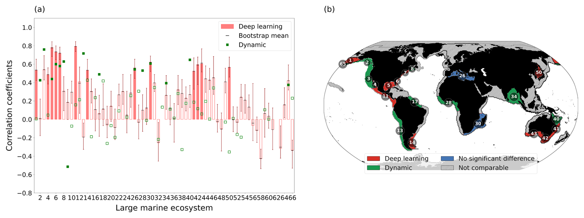
Figure 5 Comparison of chlorophyll prediction skill between deep learning and dynamic models across Large Marine Ecosystems (LMEs). (a) Correlation coefficients between satellite-observed and predicted annual mean chlorophyll anomalies at a 1-year lead time. Red bars show the deep learning model correlation; filled bars indicate significance at p<0.10. Error bars show the 95 % bootstrap confidence interval from a double bootstrap procedure accounting for both ensemble and temporal sampling uncertainty, with black dashes indicating the bootstrap mean. Green markers show the dynamic model correlation (1998–2017); filled markers indicate significance at p<0.10. (b) Map comparing prediction skill. Red shading indicates LMEs where the deep learning model significantly outperforms the dynamic model (bootstrap p<0.05) or is the only model with significant skill. Green indicates the same for the dynamic model (bootstrap p>0.95). Blue indicates LMEs where neither model significantly outperforms the other. Hatched regions indicate LMEs where both models lack significant skill or data are unavailable.

A categorical global map of relative performance (Fig. 5b) reveals distinct regional patterns. The deep learning model showed superior skill along the US coast (LMEs 5, 6, 7), the Pacific Central-American coast (LME 11), and the Indo-Australian coast (LMEs 42, 43). These regions exhibit complex chlorophyll-SST relationships that likely reflect the integrated effects of multiple environmental drivers. The data-driven approach of deep learning appears well-suited to identifying predictive patterns in these surface variables without requiring explicit parameterization of underlying processes. Feature attribution analyses further support this interpretation, consistently highlighting the contributions of climate-sensitive predictors such as surface chlorophyll and SST (Amorim et al., 2021; Liu et al., 2025).

Conversely, the dynamical model showed superior skill in the Pacific Eastern Boundary Upwelling Systems, including the Humboldt (LME 13) and California (LME 3) Currents. These regions are strongly influenced by wind-driven upwelling and episodic vertical nutrient fluxes, which are explicitly resolved in dynamical models with process-based parameterizations. While surface chlorophyll can partially reflect subsurface variability, especially in regions with coherent thermocline dynamics (Park et al., 2018a), such signals may be too intermittent or weakly expressed at the surface in those upwelling zones. This limits the ability of surface-based predictors to capture the timing and magnitude of upwelling-driven productivity variations, and likely contributes to the superior performance of the dynamical model in these physically dominated systems.

Overall, the results here suggest that deep learning and dynamical approaches offer complementary strengths across different oceanographic regimes. The deep learning model performed well in coastal LMEs characterized by complex and nonlinear dynamics, where data-driven pattern recognition provides an advantage, while the dynamical models excelled in upwelling-dominated systems where explicit representation of subsurface processes is critical.

3.5 Exploratory analysis of fish catch predictability

The successful prediction of chlorophyll anomalies in many coastal LMEs suggests that CNN-derived forecasts may serve as a predictable bottom-up driver of fisheries variability, motivating an exploratory assessment of chlorophyll–fisheries linkages. For each LME in which the CNN demonstrated significant chlorophyll prediction skill, the ten most harvested species were identified, and linear regression was applied to assess chlorophyll–catch associations at lag 0 (same year) and lag 1 (preceding year). Species–LME combinations were retained where statistically significant correlations were found, and supporting ecological literature suggested a plausible bottom-up forcing mechanism.

The results revealed statistically significant associations across diverse species and regions (Fig. 6). Contemporaneous relationships (lag=0) were found in the Pacific Central-American Coastal LME (LME 11) for South American pilchard (Sardinops sagax) and skipjack tuna (Katsuwonus pelamis), both of which are known to respond sensitively to ENSO-driven productivity fluctuations in convergence zones (Lehodey et al., 1997; Kim et al., 2020).

Lagged relationships (lag=1) emerged for species whose population dynamics are shaped by prior-year environmental conditions: northern white shrimp (Litopenaeus setiferus) in the Southeast U.S. Continental Shelf (LME 6), whose juvenile recruitment depends on antecedent temperature and productivity (Diop et al., 2007). A similar lagged relationship was observed for Japanese jack mackerel (Trachurus japonicus) in the East Sea (LME 50), potentially reflecting sensitivity to prior-year productivity during early life stages (Takahashi et al., 2016, 2022). Yellowfin tuna (Thunnus albacares) in the East Central Australian Shelf (LME 41) also showed a significant lagged correlation, consistent with the established association between tuna distribution and productivity-driven prey aggregation in the East Australian Current system (Young et al., 2011). These results show the potential of incorporating chlorophyll-based forecasts into fishery prediction frameworks. They also highlight the importance of accounting for species-specific life histories and ecological mechanisms when evaluating forecast performance across diverse ecosystems.

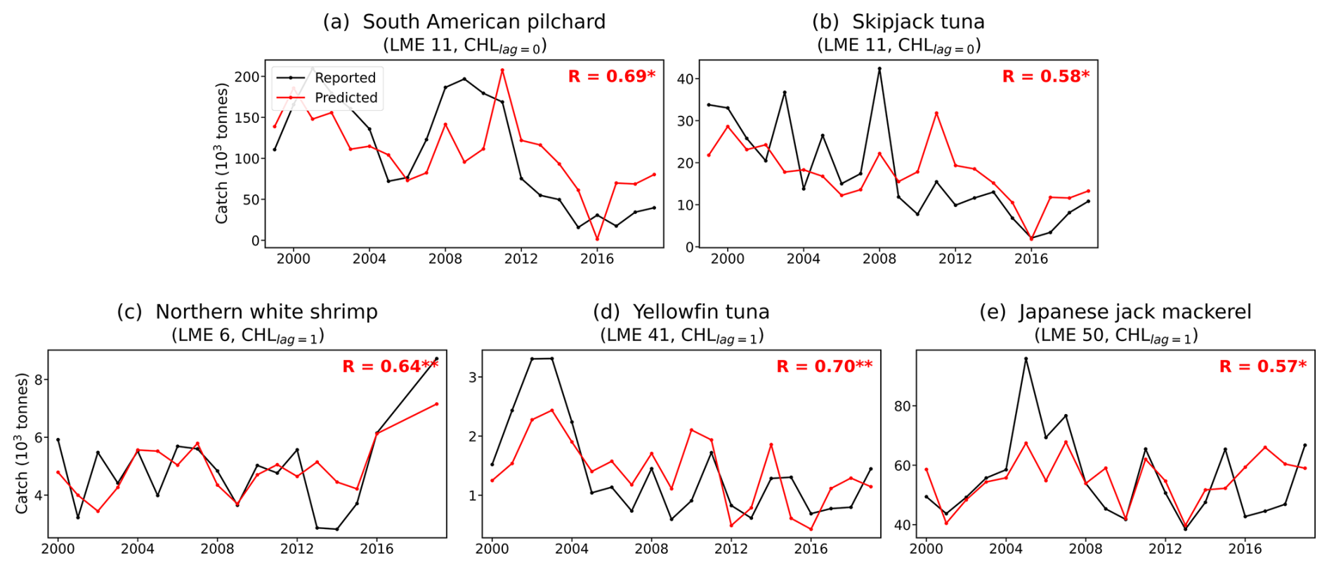
Figure 6 Prediction skill for annual fish catch of individual species in selected Large Marine Ecosystems (LMEs). (a–e) Time series of reported (black) and estimated (red) annual fish catch (tonnes). (a) South American pilchard, LME 11, lag=0. (b) Skipjack tuna, LME 11, lag=0. (c) Northern white shrimp, LME 6, lag=1. (d) Yellowfin tuna, LME 41, lag=1. (e) Japanese jack mackerel, LME 50, lag=1. lag=0 and lag=1 indicate regression against CNN-predicted chlorophyll of the same year and the preceding year, respectively. Asterisks denote statistical significance (* p<0.1, ** p<0.05).

4 Conclusion and Discussion

Regional chlorophyll variability in LMEs is often modulated by basin-scale to global-scale spatial patterns associated with large-scale climate variability, yet ESM-based dynamical forecasts at the LME scale remain constrained by limited observational records, structural uncertainty, and high computational cost. To address this, we developed a CNN based deep learning framework that predicts LME-mean chlorophyll anomalies using global SST and chlorophyll fields. By leveraging the large-scale spatial patterns that modulate regional variability, this approach achieves skillful annual chlorophyll predictions across diverse oceanographic regimes in global LMEs. We applied interpretability analysis to monthly prediction skill in two representative LMEs selected for their well-documented connections to large-scale climate variability. The results revealed that this skill arises from physically interpretable signals, including ENSO-driven SST variability and wintertime reemergence mechanisms. This suggests that statistical learning can internalize aspects of coupled physical-biogeochemical dynamics from training data. Systematic sensitivity analyses further showed that successful data-driven ecosystem prediction requires careful consideration of both model architecture (e.g., kernel size, activation functions) and input data characteristics (e.g., horizontal resolution, log-transformation, and variable selection). Notably, models using surface chlorophyll as input achieved comparable or higher prediction skill than models using subsurface temperature (0–300 m average). This suggests that surface chlorophyll anomalies encode information about subsurface ocean states through the physical linkage between nutrient supply, vertical mixing, and phytoplankton growth (Park et al., 2018a; Lim et al., 2022; Lee et al., 2024).

A further motivation of this study was to assess whether a data-driven approach can complement ESM-based dynamical predictions at the LME scale. Comparisons with an ESM-based dynamical prediction system revealed regional differences in forecast skill, providing insight into the observability of marine ecosystem drivers. The deep learning model excelled in regions dominated by large-scale climate variability, where surface signals of coupled physical-biogeochemical interactions are well captured by satellite observations. However, performance limitations in eastern boundary systems highlighted the challenges of predicting large coastal ecosystems strongly influenced by subsurface processes that may not be consistently detectable at the surface. These findings emphasize that forecast skill depends not only on model design but also on the extent to which key ecological drivers are represented in available data. A key practical advantage of the deep learning approach is computational efficiency. Once trained, the CNN produces forecasts in seconds, compared to the thousands of simulation years required for dynamical retrospective forecasts (e.g., Park et al., 2019). This enables rapid generation of large ensembles and facilitates operational applications where timely forecast delivery is essential.

Beyond chlorophyll prediction itself, a broader motivation is to support climate-informed marine resource management. The demonstrated links between predicted chlorophyll anomalies and fish catch variability provide exploratory evidence for potential linkages between biogeochemical forecasting and marine resource management. Statistically significant correlations were found for both contemporaneous responses (skipjack tuna, South American pilchard) and lagged responses (northern white shrimp, yellowfin tuna, jack mackerel), patterns consistent with known life history traits and recruitment dynamics. However, several important caveats must be acknowledged. Species–LME combinations were selected based on two conditions: significant CNN chlorophyll prediction skill in the LME, and a statistically significant correlation between predicted chlorophyll and catch anomalies. The latter was further restricted to species with a plausible bottom-up forcing mechanism suggested by ecological literature. While this structured selection reduces the risk of purely spurious associations, the analysis relies on bottom-up environmental forcing alone and does not account for top-down effects on reported catch data, such as fishing effort, management interventions, fleet behavior, and reporting practices. We note that the regression relationships are fitted over the entire analysis period and thus represent in-sample associations, consistent with the exploratory nature of this analysis. Although these relationships were identified in only a subset of LMEs, they demonstrate the feasibility of integrating environmental forecasts into fisheries applications. Such applications will require careful consideration of species-specific ecological mechanisms and regional oceanographic contexts. Developing cross-validated prediction frameworks and incorporating additional biogeochemical variables, such as NPP or trophic processes, would be valuable directions for future work.

Several limitations should also be acknowledged. Training on CMIP6 simulations creates an inherent ceiling on CNN performance tied to the fidelity of the training data. Training on diverse multi-model ensembles has been shown to improve generalization beyond the limitations of individual models in similar deep learning frameworks (Guo et al., 2025). Building on this principle, our multi-model training strategy (16 CMIP6 models) leverages the diversity of model physics and biogeochemical parameterizations across the ensemble, which is expected to reduce sensitivity to the biases of any individual model. We additionally incorporated the GFDL-ECDA reanalysis, which assimilates observational constraints into the physical ocean state. As shown in the sensitivity experiments (Sect. 3.1), excluding the reanalysis and training on CMIP6 models alone resulted in modestly lower prediction skill, suggesting that observationally-constrained training data helps anchor the CNN to more realistic physical–biogeochemical relationships. Nevertheless, biases shared across the CMIP6 ensemble, such as limited representation of coastal processes and common biogeochemical parameterization assumptions, may still propagate to CNN predictions, and the forecasts should be interpreted with this limitation in mind. As ESMs continue to improve across successive generations, with documented progress in marine biogeochemistry from CMIP5 to CMIP6 (Séférian et al., 2020), such biases are expected to diminish, offering a pathway toward further gains in prediction skill for data-driven frameworks like ours.

Our 1°×1° input resolution does not resolve fine-scale coastal processes such as submesoscale upwelling, river plume dynamics, and nearshore bathymetric effects. Satellite-derived chlorophyll observations also carry substantial uncertainties in coastal waters due to optical complexity. Furthermore, the clear-sky sampling bias of satellite observations introduces an inconsistency with the all-sky ESM training data, which our unified masking strategy mitigates but does not fully eliminate. These factors, combined with large spatial variability of chlorophyll within LMEs, mean that our LME-mean predictions are most informative for basin-scale environmental conditions rather than localized ecosystem responses.

Another limitation relates to the model's spatial constraints and variable selection. The model treated LMEs as independent units, potentially overlooking cross-basin connectivity and anomaly propagation that could enhance predictive skill across regional boundaries. Other key physical drivers, such as wind stress, mixed-layer depth, photosynthetically available radiation, and vertical nutrient gradients, were not systematically evaluated as CNN inputs. SST and chlorophyll were selected as inputs because both variables have consistent availability across the CMIP6 multi-model ensemble and nearly two decades of near-global satellite observations. This makes them a natural starting point for data-driven biogeochemical forecasting. SST additionally serves as an integrated proxy for multiple physical drivers, including upper-ocean stratification and circulation. Regions where local processes dominate chlorophyll variability may nonetheless benefit from incorporating additional physical drivers in future extensions.

Finally, the current zero-filling approach for missing satellite data was shown to be effective through SHAP analysis, with near-zero contributions from masked regions (Fig. 4b and d). This approach could be extended in future work through alternative approaches such as missingness indicator channels or masked loss functions. Future research should address these limitations by incorporating additional physical variables and exploring architectures that retain spatial context, such as encoder-decoder frameworks or graph-based networks, to better represent cross-basin connectivity and process-dominated systems. Moreover, hybrid frameworks that combine machine learning with dynamical simulations, leveraging expanding Earth observation archives, offer a promising path toward transparent, flexible, and operational biogeochemical forecasting systems capable of supporting adaptive, climate-informed marine resource management.