Improving terrestrial carbon flux simulations with machine learning and global Earth observations

The land carbon cycle currently absorbs about one-third of anthropogenic CO₂ emissions, but multi-model studies project a future weakening of this sink and a possible shift to a carbon source. Large inter-model differences limit confidence in these projections, and some of these discrepancies may arise from parameter uncertainty. Parameter optimization using global Earth observations could reduce this uncertainty, but it is computationally expensive and complicated by equifinality, where different parameter combinations yield similar performance through compensating effects. To address these challenges, this study uses a genetic algorithm to optimize 28 model parameters against 13 global observation datasets. A Gaussian process emulator is then used to approximate the relationship between model performance and parameter values, explore equifinality, and identify alternative parameter sets with comparable performance. These sets are used to generate an ensemble of simulations, providing an estimate of uncertainty associated with parameter optimization. Results show that optimization improves global model performance, especially for leaf area index and gross primary productivity (GPP). Optimized global GPP decreases by 5 %, resulting in a 61 % reduction in global net biome productivity (NBP) compared with the default simulation. While equifinality arises from compensating effects among many parameters, the reductions in GPP and NBP remain robust and are confirmed by the emulator-derived parameter sets. These findings highlight that parameter tuning can substantially alter carbon fluxes, and modelling groups should integrate advanced parameter optimization frameworks into their development cycle.

1 Introduction

The global carbon cycle has the potential to both mitigate and amplify climate change. The Earth's terrestrial biosphere currently absorbs more CO₂ than it releases, making it a net carbon sink (Friedlingstein et al., 2025). This sink sequesters about one-third of all anthropogenic CO₂ emissions, acting as a negative feedback mechanism that mitigates climate change. Paleoclimate data on the other hand shows that an increase in atmospheric CO₂ concentration raises global mean surface temperatures, which in turn drives further increases in atmospheric CO₂ (van Nes et al., 2015). Here, the carbon cycle is acting as a positive feedback mechanism, amplifying a warming trend. The empirical evidence for a positive carbon cycle feedback raises the question whether the terrestrial carbon sink will eventually transition from a net carbon sink to a net carbon source as global mean surface temperatures continue to rise.

Empirical data from the global carbon flux monitoring network indicate that over the past decade, plants have reached the thermal maximum for photosynthesis during the three warmest months each year (Duffy et al., 2021). The same study suggests that as temperatures rise, respiration rates are expected to continue increasing while photosynthesis declines, potentially reducing the land sink strength by nearly half over the next two decades under a business-as-usual emission scenario.

Climate models can help separate the effects of changes in atmospheric CO₂ concentration (carbon-concentration feedback) and climate (carbon-climate feedback) on land-atmosphere carbon fluxes. Results from the latest generation of climate models, known as Earth System Models (ESMs), indicate that the carbon-concentration feedback is negative, meaning the land acts as a net carbon sink. In contrast, the carbon-climate feedback is positive, suggesting the land functions as a net carbon source (Arora et al., 2020). When both feedback mechanisms act in concert, ESMs project that the land will continue to act as a carbon sink by the end of the 21st century, but the strength of this sink is subject to substantial uncertainties, ranging from about 2 to 7 Pg C yr⁻¹ for a fossil-fuel-intensive scenario (Canadell et al., 2021). Longer-term simulations with a set of five ESMs and one ESM of intermediate complexity project that the terrestrial biosphere will switch from a carbon sink to either a neutral state or a carbon source by the year 2300 (Koven et al., 2022). Here as well, the inter-model differences remain substantial, ranging between −7 to 0 Pg C yr⁻¹.

The annual publication of the global carbon budget (GCB) provides regular updates on historical carbon fluxes and the strength of the terrestrial carbon sink (Friedlingstein et al., 2025). This carbon sink is estimated using an ensemble of terrestrial biosphere models referred to as the trends in the land carbon cycle project (TRENDY) ensemble. In the context of TRENDY, the models are driven offline with quasi-observed meteorological data. However, many of the TRENDY models also serve as the land surface components of fully coupled ESMs used for the future projections discussed above. Comparing the TRENDY ensemble against a wide range of global Earth observations shows that while model performance is generally reasonable, substantial room for improvement remains (Seiler et al., 2022). Notably, there is a large inter-model spread in net biome productivity (NBP) and gross primary productivity (GPP), and most models tend to overestimate the leaf area index across all latitudes when compared to multiple remote sensing datasets (their Fig. 2).

To summarize, empirical data and numerical modelling both indicate that the strength of the land carbon sink will decline as temperatures rise. However, the rate of this decline and a potential shift from a carbon sink to a carbon source remain highly uncertain. The current generation of models that simulate terrestrial carbon fluxes is still subject to considerable biases and large inter-model differences. Improving model performance for the historical period may yield more reliable future projections. One source of uncertainty arises from parameters that are not fundamental constants, but whose values depend on environmental conditions. The true values of these free parameters are often unknown and must be selected within physically consistent uncertainty ranges. While traditional approaches to parameter tuning rely on expert judgment, recent advancements in machine learning, coupled with increasing computational power and the availability of global Earth observations, have opened up new opportunities for more systematic and efficient parameter tuning.

A common approach for parameter optimization is referred to as data assimilation. Data assimilation has a long history in weather forecasting, where it uses global Earth observations to estimate the initial conditions of state variables such as temperature, humidity, and wind speed. However, the same technique can be used to optimize parameters, essentially by treating model parameters as initial conditions. The technique can use a variety of data streams, ranging from local in-situ observations to globally gridded datasets at daily, monthly, and annual time scales (MacBean et al., 2022). For instance, Kuppel et al. (2012) optimized 21 model parameters using daily carbon and energy fluxes from 12 eddy covariance measurement sites, reducing the model's root-mean-square error by 22 %. MacBean et al. (2018) optimized 17 parameters using monthly satellite-derived measures of sun-induced chlorophyll fluorescence (SIF), reducing global mean annual GPP biases from 46 % to 25 %. Bacour et al. (2023) optimized 15 parameters using eddy covariance data, satellite-derived normalized difference vegetation index, and atmospheric CO₂ concentration data measured at stations, resulting in a stronger global carbon sink that better aligns with estimates from the GCB. Their study also found that parameter optimization is more effective when multiple data streams are used simultaneously during the optimization process.

The examples above apply to the Organising Carbon and Hydrology In Dynamic Ecosystems (ORCHIDEE) model, which forms the land surface component of the Institute Pierre Simon Laplace (IPSL) ESM (IPSL-CM5). The approach uses a Bayesian framework that iteratively minimizes a cost function using a gradient-based method referred to as the Limited-memory Broyden-Fletcher-Goldfarb-Shanno Bound (L-BFGS-B) algorithm (Tarantola, 2005; Byrd et al., 1995). This widely used algorithm has also been applied to other models, such as the Joint UK Land Environment Simulator (JULES) (Raoult et al., 2016) and the Jena Scheme for Biosphere-Atmosphere Coupling in Hamburg (JSBACH) (Schürmann et al., 2016). Other commonly used optimization algorithms include the adaptive Metropolis - Hastings - based Markov Chain Monte Carlo algorithm, which has been employed for parameter estimation in the Lund–Potsdam–Jena General Ecosystem Simulator (LPJ-GUESS) (Kallingal et al., 2024), and the Ensemble Adjustment Kalman Filter, which has been applied to the Community Land Model (CLM) (Fox et al., 2018).

The primary bottleneck in parameter optimization is its high computational cost, as optimization requires many iterations to progressively improve model performance. These costs make it difficult to fully explore equifinality, the possibility that similar model performance can arise from different parameter combinations due to compensating parameter effects (Raoult et al., 2025). To overcome this limitation, this study employs a Gaussian process emulator to approximate the relationship between model performance and parameter values. Because the emulator incurs negligible computational cost, it enables a systematic exploration of equifinality and the identification of multiple parameter sets with similarly high performance. These parameter sets are then used to generate an ensemble of simulations, providing an estimate of the uncertainty associated with parameter optimization.

The approach is implemented using the Canadian Land Surface Scheme Including Biogeochemical Cycles (CLASSIC) (Melton et al., 2020), which serves as the land surface component of the Canadian Earth System Model (CanESM) (Swart et al., 2019) and contributes to the TRENDY ensemble (Friedlingstein et al., 2025). Although recent efforts have advanced CLASSIC parameter optimization (Gauthier et al., 2025), a general-purpose optimization framework, capable of targeting any subset of CLASSIC parameters and integrating diverse observational data streams, has yet to be developed. Whereas previous studies typically constrain model parameters using observations over relatively short time periods (Peylin et al., 2016; Schürmann et al., 2016; MacBean et al., 2018), the optimization in this study is performed over a much longer time span (1701–2020), allowing sufficient time for parameter effects to fully manifest. In addition, the optimization simultaneously targets multiple variables using multiple observational data streams per variable. This approach helps account for observational uncertainty and reduces the risk of overfitting to any single dataset.

The following sections detail the methods used in this study, including a description of the model, simulation protocol, model parameters, machine learning algorithm, evaluation framework, equifinality approach, and the Gaussian process emulator. The results section begins by evaluating the reliability of the approach using synthetic data, followed by an analysis of how optimization affects parameter values and model performance for a subset of 360 grid cells. Next, I use the emulator to explore the nature of equifinality and to generate alternative parameter sets. I then apply the optimized and emulated parameter sets to all land grid cells and assess global model performance. Finally, I examine the impact of optimization on globally accumulated gross primary productivity and net biome productivity. The discussion section highlights key findings, addressing both the potential and limitations of my approach. Finally, I discuss the importance of improving estimates of future carbon fluxes for climate change mitigation policies and emphasize the need for climate modelling groups to integrate advanced parameter optimization methods into their model development cycle.

2 Methods

2.1 Land Surface Model

The Canadian Land Surface Scheme Including Biogeochemical Cycles (CLASSIC) forms the land surface component of the Canadian Earth System Model (CanESM) (Melton et al., 2020; Swart et al., 2019). CLASSIC's physical component, known as CLASS, partitions the land surface into four distinct subareas: bare ground, snow-covered ground, canopy-covered ground, and snow-covered canopy. The model solves the energy balance equations for the canopy layer and the underlying ground separately. The canopy comprises a single layer that encompasses four plant functional types (PFTs): needleleaf trees, broadleaf trees, grasses, and crops. The offline model configuration used here has 20 soil layers ranging from 10 layers of 0.1 m thickness, gradually increasing to a 30 m thick layer for a total ground depth of over 61 m. Water fluxes are computed within the permeable soil depth of the ground column, excluding underlying bedrock layers. Temperature calculations encompass both soil and bedrock layers. Furthermore, the model computes the temperature, mass, albedo, and density of the single-layer snowpack, as well as the temperature, interception, storage of rain and snow on the canopy, and the temperature and depth of ponded water on the ground surface.

CLASSIC's biogeochemical component, referred to as CTEM, is a dynamic vegetation model coupled to CLASS. CLASS provides essential physical land surface data, including soil moisture, soil temperature, and net radiation, which are used by CTEM to simulate photosynthesis in response to [CO₂]. CTEM accounts for three living vegetation components (leaves, stem, and roots) and two dead carbon pools (litter and soil). These five carbon pools are monitored for nine PFTs, mirroring the four PFTs from CLASS. For instance, needleleaf trees are subdivided into deciduous and evergreen types, while broadleaf trees are categorized as cold and drought-deciduous and evergreen types. Additionally, crops and grasses are differentiated based on their photosynthetic pathways, resulting in C₃ and C₄ versions. The names and corresponding acronyms of the PFTs used in this study are needleleaf evergreen tree (NDL.EVG), needleleaf deciduous tree (NDL.DCD), broadleaf evergreen tree (BDL.EVG), broadleaf deciduous cold tree (BDL.DCD.CLD), broadleaf deciduous dry tree (BDL.DCD.DRY), C₃-photosynthesis grass (GRASS.C3), C₄-photosynthesis grass (GRASS.C4), C₃-photosynthesis crop (CROP.C3), and C₄-photosynthesis grass (CROP.C4). The spatial allocation of PFTs is predefined.

Model inputs that vary in time include seven meteorological variables (downwelling SW radiation, downwelling LW radiation, surface precipitation rate, surface air pressure, specific humidity, air temperature, and wind speed), [CO₂], land cover, and population density. Another input variable is lightning density, which is based on climatological monthly values. The main processes simulated by the biogeochemical component of CLASSIC and that are used in my study include photosynthesis, canopy conductance, tissue turnover, allocation of carbon, phenology and crop harvesting (Arora and Boer, 2004), dynamic root distribution (Arora and Boer, 2003), maintenance, growth and heterotrophic respiration (Melton et al., 2015), wildfires (Arora and Boer, 2005; Arora and Melton, 2018), and land use change (Arora and Boer, 2010). Note that the model's nitrogen cycle (Asaadi and Arora, 2021; Kou-Giesbrecht and Arora, 2022) has been turned off.

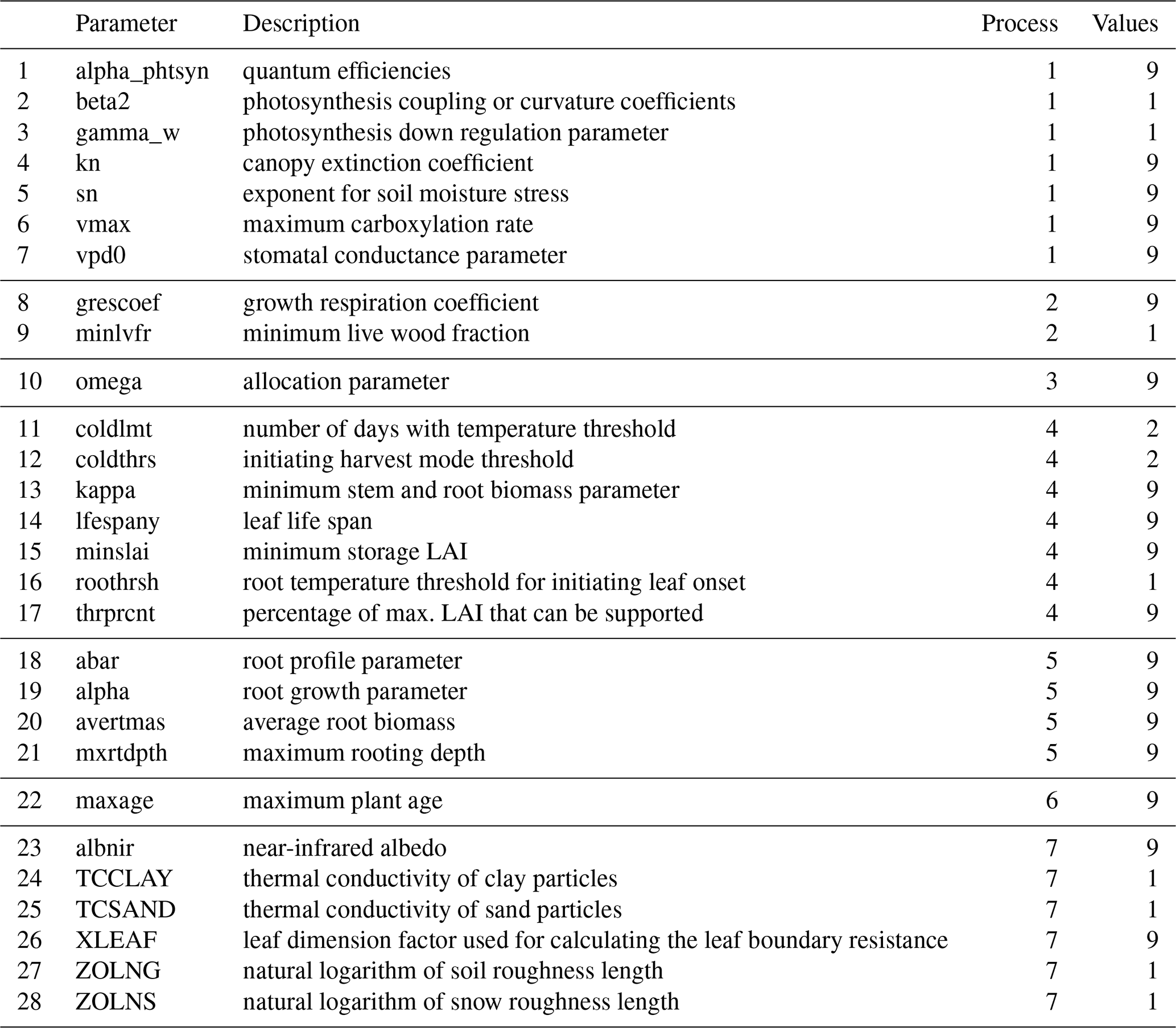
Table 1 Parameters that participate in the optimization, where Process refers to (1) photosynthesis, (2) autotrophic respiration, (3) allocation (4) phenology, (5) rooting, (6) mortality (7) physical, and Values denotes the number of values per parameter.

2.2 Parameter Uncertainty Ranges

There are about 100 CLASSIC model parameters, depending on the exact model configuration. Deepak et al. (2025) conducted a Global Sensitivity Analysis for CLASSIC, identifying the most influential parameters for carbon and turbulent heat fluxes for seven major biomes. While 20 parameters were consistently influential, variations across sites increased the total to 28 parameters. Many parameters have multiple values to account for different PFTs. Parameters with nine values differentiate among nine PFTs, while those with four values distinguish between needleleaf trees, broadleaf trees, grasses, and crops. Parameters with two values separate trees from grasses or crops. As a result, the total number of parameter values tuned increases to 165. The present study optimizes these 165 parameters within their respective uncertainty ranges (Table 1). The two parameters that were frequently most influential were the maximum carboxylation rate (v_max) and the canopy extinction coefficient (k_n). Given the importance of both parameters, I have refined their respective uncertainty ranges using empirical data provided by the TRY database (Kattge et al., 2019) and literature.

The TRY data base provides v_max values for different plant species. Classifying these species into PFTs, I obtained PFT-specific values for needleleaf evergreen trees (n=998), needleleaf deciduous trees (n=9), broadleaf evergreen trees (n=2456), broadleaf deciduous trees (n=3813), C₃ metabolism herbs/grasses (n=965), and C₄ metabolism herbs/grasses (n=11). The PFT classification does not distinguish between cold versus dry broadleaf deciduous trees or grasses versus crops. Therefore, I applied the uncertainty ranges from broadleaf deciduous trees to both cold and dry broadleaf deciduous trees. Likewise, I applied the C₃ metabolism herbs/grasses to both C₃ grasses and C₃ crops, and similarly for C₄ metabolism herbs/grasses. For most PFTs, I defined the uncertainty range as the interquartile range of the observations. However, in the case of needleleaf deciduous trees, C₄ grasses and C₄ crops, I used the total observed range as the uncertainty range due to the small sample size. For C₄ grasses and crops, I set the lower bound of the uncertainty range to the model's default value, which was lower compared to the smallest observed value.

The k_n uncertainty ranges are based on a meta-analysis presented by Zhang et al. (2014). Their study provides means and standard deviations of k_n during the whole growth season for sites located in needleleaf forest (n=15), broadleaf forest (n=9), grassland (n=17) and croplands (n=35). These values are utilized as uncertainty ranges for the PFTs. For C₃ crops, I selected the default model parameter as the lower bound, which was lower compared to the value provided by the aforementioned meta-analysis. All other parameter uncertainty ranges were obtained from Deepak et al. (2025), who determined these ranges from literature and expert judgement.

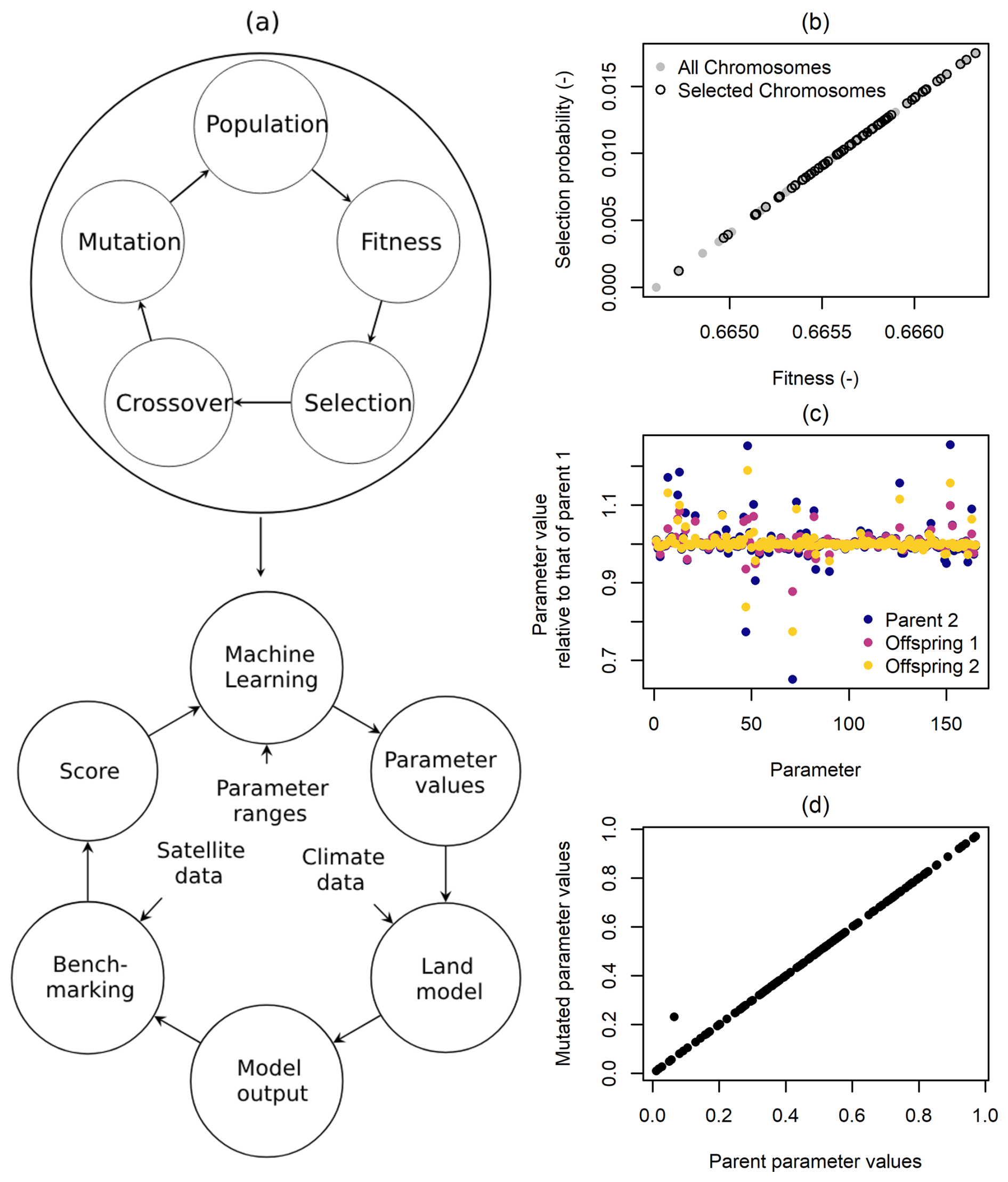
Figure 1 (a) Parameter optimization flowchart, (b) selection, (c) crossover, and (d) mutation.

2.3 Model Parameter Optimization

Model parameter optimization is an iterative process in which a machine learning algorithm identifies parameter values that improve model performance over time (Fig. 1a). The algorithm initially proposes multiple sets of randomly selected parameter values within their prescribed uncertainty ranges. These values, combined with historical climate data, are used to conduct simulations with CLASSIC for a selection of grid cells. The resulting model outputs are then compared against global Earth observations to assess how well each parameter set performs. Based on this evaluation, the machine learning algorithm proposes a new set of parameter values aimed at improving model performance. This iterative process continues until no further improvement is observed. Once the optimal parameter values are determined, I run the model globally using the optimized parameter values during the spinup, transient, and projected future simulations. The next few paragraphs describe how the machine learning algorithm works.

Model optimization can be performed using a variety of machine learning algorithms, each with its own strengths and limitations. This application employs a Genetic Algorithm (GA), implemented in the open-source programming language R by Scrucca (2013). A key advantage of GAs is their ability to explore a broad solution space, reducing the risk of getting trapped in local optima (Eiben and Smith, 2015). Additionally, they do not require the objective function to be continuous and can be efficiently parallelized on high-performance computing systems.

The defining feature of GAs is their ability to optimize parameter values by mimicking biological evolution. In this process, the set of parameters to be optimized is analogous to a chromosome, with each parameter representing a gene (Goldberg, 2012). The main steps of a GA are (i) selection of a population, (ii) crossover, and (iii) mutation. As a first step, the user specifies model parameter uncertainty ranges for all parameters that participate in the optimization process. In this adoption of a GA, I normalize parameter values such that they become dimensionless and vary between zero and one:

$$\begin{array}{}\text{(1)}& \widehat{x_i}={\displaystyle \frac{x_i-min}{max-min}},\end{array}$$

where $\widehat{x_i}$ is the normalized value of the parameter i, x_i is the actual parameter value, and min and max are the parameter's lower and upper boundary values, respectively. Early versions of GAs represented parameter values in binary form (Goldberg, 2012). However, I use the more common real-value representation, working directly with normalized parameter values. Each parameter is represented as an element in the vector $X=(x_{\mathrm{1}},x_{\mathrm{2}},\mathrm{\dots },x_n)$, where each parameter x_i falls within its uncertainty range, spanning from zero to one. This vector represents the chromosome, with individual parameter values serving as genes.

The GA starts the optimization by producing a population of n chromosomes, where each chromosome consists of genes with values that are randomly chosen within the uncertainty range of 0 to 1. The population forms the first generation in the optimization process. The fitness function runs CLASSIC n-times using each of the n chromosomes as an input. The GA then calculates the relative fitness of each chromosome, as detailed in Sect. 2.4. This fitness value determines the selection of parent chromosomes, with well-performing chromosomes having a higher probability of being chosen. Selection can be performed in various ways. In this application, I use a method known as fitness-proportional selection with fitness linear scaling (Scrucca, 2013), where the selection probability P_i of a chromosome is given as:

$$\begin{array}{}\text{(2)}& P_i={\displaystyle \frac{f_i^{\prime }}{{\sum }_{j=\mathrm{1}}^N{f}_j^{\prime }}},\end{array}$$

where $f_i^{\prime }$ is the linearly scaled fitness of an individual chromosome i and N is the population size. The linearly scaled fitness is given by:

$$\begin{array}{}\text{(3)}& f_i^{\prime }=a\cdot f_i+b,\end{array}$$

where f_i is the fitness of chromosome i and a and b are scaling coefficients that are computed as follows:

$$\begin{array}{}\text{(4)}& {\displaystyle }a=\overline{f}/\mathit{\delta },\text{(5)}& {\displaystyle }b=-f_{\min }\cdot \overline{f}/\mathit{\delta },\text{(6)}& {\displaystyle }\mathit{\delta }=\overline{f}-f_{\min },\end{array}$$

where $\overline{f}$ and f_min are the mean and minimum fitness of all chromosomes, respectively. Once each chromosome has an assigned selection probability, the population is then randomly sampled (with replacement) where chromosomes with a higher selection probability are more likely to be selected. This is illustrated in Fig. 1b, which shows the chromosomes being selected along with their corresponding fitness values. As a result, the best-performing strings get more copies, the average-performing strings stay even, and the worst-performing strings die off (Goldberg, 2012).

Selection alone does not improve solutions. The exploitation of current solutions is achieved through crossover, which can be performed in various ways. The method I have adopted is local arithmetic crossover, where crossover is applied to all genes, but the extent to which the offspring gene is influenced by Parent 1 or Parent 2 varies from gene to gene (Scrucca, 2013):

$$\begin{array}{}\text{(7)}& {\displaystyle }{O}_{\mathrm{1}}=\mathit{\alpha }{P}_{\mathrm{1}}+(\mathrm{1}-\mathit{\alpha })P_{\mathrm{2}},\text{(8)}& {\displaystyle }{O}_{\mathrm{2}}=\mathit{\alpha }{P}_{\mathrm{2}}+(\mathrm{1}-\mathit{\alpha })P_{\mathrm{1}},\end{array}$$

where α is a random value taken from a uniform distribution spanning between zero and one. Each parameter receives a different α value. Figure 1c shows how the values of Parent 1 and Parent 2 differ from Offspring 1 and Offspring 2. Here, the values of each gene, represented as dots, are divided by the corresponding values from Parent 1. The figure demonstrates that the offspring values are bounded by the corresponding values from the parents. However, the exact location varies, as α differs among genes.

Next, the GA performs mutations that randomly alter genes. The purpose of mutation is to explore the whole parameter space, preventing the optimization from being trapped in a local maximum. The mutation function I used is the uniform random mutation, which randomly modifies one gene per chromosome (Fig. 1d). After selection, crossover, and mutation, the new generation of chromosomes is used as inputs for the fitness function, and the process starts from the beginning.

The building block hypothesis offers an interpretation of why the seemingly random process of selection, crossover and mutation leads to parameter optimization. At the core of this hypothesis lies a concept referred to as schema. A schema is a parameter vector that restricts some parameters to subranges that are more narrow than the uncertainty ranges (e.g. $\mathrm{0.3}<x_i<\mathrm{0.5}$ rather than $\mathrm{0}<x_i<\mathrm{1}$). Schemata can differ in length, order, and fitness. A short schema constrains a small but meaningful subset of parameters. A low-order schema constrains parameters moderately, avoiding both excessive precision and excessive freedom. A high-fitness schema contains solutions that perform above average. The building block hypothesis states that short, low-order, and high-fitness schemata are more likely to propagate over generations (Eiben and Smith, 2015). These short, low-order, and high-fitness schemata form building blocks, which GAs assemble to create increasingly optimal solutions over time. Selection increases the proportion of high-fitness building blocks over generations. Crossover recombines information from two parent building blocks to create new offspring. Mutation introduces random changes to parameters, helping the algorithm explore new areas of the search space. The repeated selection, recombination, and mutation refine and assemble building blocks, leading to increasingly optimized solutions.

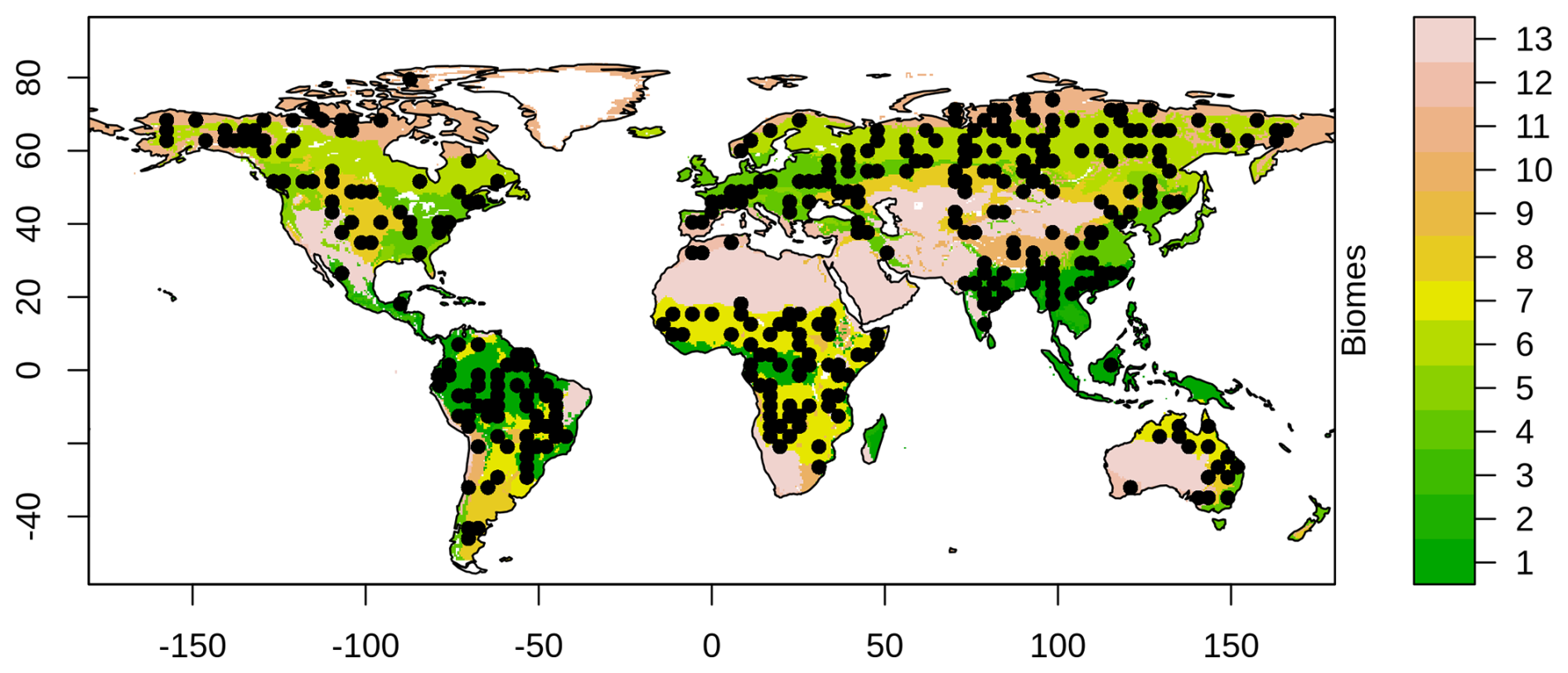
Figure 2 Locations of 360 randomly selected model grid cells used for parameter optimization. The number of selected grid cells per biome is weighted by the biome's area, including (1) Tropical and Subtropical Moist Broadleaf Forests, (2) Tropical and Subtropical Dry Broadleaf Forests, (3) Tropical and Subtropical Coniferous Forests, (4) Temperate Broadleaf and Mixed Forests, (5) Temperate Conifer Forests, (6) Boreal Forests/Taiga, (7) Tropical and Subtropical Grasslands, Savannas and Shrublands, (8) Temperate Grasslands, Savannas and Shrublands, (9) Flooded Grasslands and Savannas, (10) Montane Grasslands and Shrublands, (11) Tundra, (12) Mediterranean Forests, Woodlands and Scrub, and (13) Deserts and Xeric Shrublands.

Parameter optimization is computationally expensive. To make the process feasible, I optimize parameters for 360 randomly selected model grid cells (Fig. 2). These grid cells are distributed across the world's major biomes, with the number of grid cells per biome proportional to the biome’s area. The number of grid cells was selected such that the optimization could be completed within two weeks of wall-clock time on the Digital Research Alliance of Canada's high-performance computing system (Rorqual). The optimization was run for 25 generations, with 100 individuals per generation, resulting in a total of 2500 simulations.

2.4 Model Evaluation

This section describes how I quantify model fitness. The approach is used as the cost function in the optimization process, as well as for measuring model performance when assessing the impact of parameter optimization on global runs. In both cases, performance is quantified using the Automated Model Benchmarking R package developed by Seiler et al. (2022), which quantifies model performance using a skill score system that is based on the International Land Model Benchmarking (ILAMB) framework (Collier et al., 2018). The method employs five scores that assess the model's annual mean bias (S_bias), monthly centralized root-mean-square-error (S_rmse), the timing of the seasonal peak (S_phase), inter-annual variability (S_iav), and spatial distribution (S_dist). The main steps for computing a score usually include (i) computing a dimensionless statistical metric, (ii) scaling this metric onto a unit interval, and (iii) computing a spatial mean. All scores are dimensionless and range from zero to one, where increasing values imply better performance. These properties allow me to average skill scores across different statistical metrics in order to obtain an overall score for each variable (S_overall). A full description of AMBER is provided by Seiler et al. (2021).

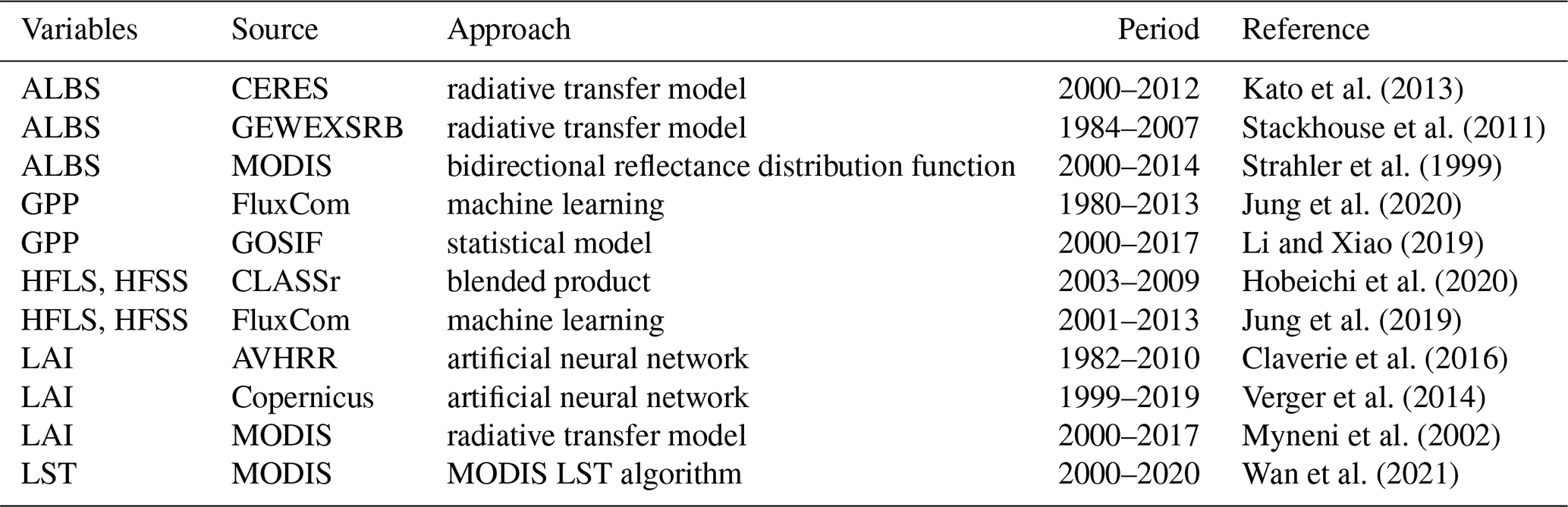
The optimization is performed for multiple data streams simultaneously using six standard land surface variables: surface albedo (ALBS), gross primary productivity (GPP), latent heat flux (HFLS), sensible heat flux (HFSS), leaf area index (LAI), and land surface temperature (LST) (Table 2). To reduce the risk of overfitting, I rely on multiple observation-based reference datasets for each variable where available. Specifically, I use three products for ALBS (CERES, GEWEXSRB, and MODIS), two for GPP (FLUXCOM and GOSIF), and two each for HFLS and HFSS (CLASSr and FLUXCOM). For LAI, I include three datasets (AVHRR, Copernicus, and MODIS), while for LST, I use a single product (MODIS). These datasets are described in Seiler et al. (2022), with full references provided in Table 2. Although this research focuses on carbon fluxes, all datasets are weighted equally because the carbon, energy, and water cycles are coupled and must be represented consistently.

Kato et al. (2013)Stackhouse et al. (2011)Strahler et al. (1999)Jung et al. (2020)Li and Xiao (2019)Hobeichi et al. (2020)Jung et al. (2019)Claverie et al. (2016)Verger et al. (2014)Myneni et al. (2002)Wan et al. (2021)

Table 2 Global Earth observations used for model evaluation, where ALBS is surface shortwave albedo, GPP is gross primary productivity, HFLS is latent heat flux, HFSS is sensible heat flux, LAI is leaf area index, and LST is land surface temperature.

The same data streams used during optimization are also used to assess model performance across all 2444 land grid cells. This global evaluation includes the 360 grid cells used during optimization because the optimization applies default parameters during the spinup and optimized parameters only during the transient period (1901–2022). In contrast, the global evaluation uses the optimized parameter set consistently during both spinup and transient periods. Therefore, it is necessary to assess model performance for all grid cells, including those used in the optimization.

To evaluate global simulations, I also compare my results against global NBP, which represents the net carbon flux between the terrestrial biosphere and the atmosphere. Although NBP is difficult to estimate directly, it can be derived as the difference between fossil fuel emissions and the atmospheric growth rate, the ocean sink, and the cement carbonation sink (Friedlingstein et al., 2025), all of which are available from 1960 onwards (see Appendix A for details).

2.5 Equifinality

The optimized parameter values may represent only one of many parameter combinations that yield near-optimal performance. One way to assess the presence of equifinality is to perform multiple optimizations with different configurations, such as varying the random number generator seeds. However, because each optimization is computationally expensive (approximately two weeks for the current setup), I instead construct a Gaussian process emulator that relates model performance to parameter values. The training data for the emulator are obtained from the genetic algorithm optimization, as described next.

Let us recall that the optimization consists of 2500 simulations over 360 grid cells. Approximately 18 % of the simulations did not complete because certain combinations of parameter values produced unphysical model states that caused the model to crash. From the remaining 2040 simulations, the simulations are ranked by performance and the lowest-performing 25 % are discarded, leaving 1530 simulations. This subset forms the training data set for constructing the emulator using the R package DiceKriging (Roustant et al., 2012). The performance of the emulator is assessed using cross-validation. For each parameter set, the corresponding performance score is removed from the training data, the emulator is refit, and the performance score is predicted. This procedure is repeated for all parameter sets.

Next, I use a Latin hypercube to sample the total parameter uncertainty space of all 165 parameters, generating 50 000 parameter sets. For each parameter set, I calculate the normalized Euclidean distance to the optimized parameter values (see Appendix B for details). Plotting the normalized Euclidean distance against the emulated AMBER scores reveals whether the model is subject to equifinality. If model performance deteriorates with increasing Euclidean distance, this suggests that the optimized parameter values correspond to a global solution. Conversely, if the two variables are not correlated and multiple parameter sets achieve performance comparable to that obtained from the genetic algorithm optimization, this indicates that the model exhibits equifinality. In this application, I first assess the relationship between Euclidean distance and AMBER score using global sampling, drawing 50 000 parameter sets from the full parameter uncertainty range. I then perform local sampling by drawing parameter values within ±10 % of the optimized parameter values, also using 50 000 parameter sets.

Finally, I investigate whether equifinality arises from compensating effects among many parameters or is driven by a smaller subset of key parameters. To assess this, I select the top 10 % of parameter sets obtained from the optimization, yielding 153 parameter sets. For each parameter, the range spanned by these 153 solutions is computed, and this reduced parameter space is sampled 5000 times using Latin hypercube sampling. The emulator is then evaluated for each of these 5000 parameter sets. From this ensemble, the top 10 % of best-performing simulations are retained, resulting in 500 parameter sets. A principal component analysis is applied to this subset to determine whether the variance in parameter space can be explained by a small number of principal components. If a few components capture most of the variance, it suggests that equifinality arises from trade-offs among a limited set of parameters. Conversely, if many components are needed to account for the variance, this indicates that the variance is distributed across numerous parameters and that equifinality is high-dimensional rather than driven by a small number of key interactions. The assessment of equifinality described above relies on a Gaussian process emulator. The theory underlying Gaussian process emulators is summarized in the next few paragraphs.

2.6 Gaussian Process Emulator

An emulator is a statistical representation of a model (Holden et al., 2015). A Gaussian process emulator is a probabilistic model for functions, such that for any finite set of inputs, the function values follow a multivariate Gaussian distribution (Rasmussen and Williams, 2008). This method is used to approximate complex functions, especially when the underlying function is expensive to evaluate directly. The function f(x) is distributed as a Gaussian process with mean function m(x) and covariance function $k(\mathit{x},{\mathit{x}}^{\mathbf{\prime }})$ (the kernel):

$$\begin{array}{}\text{(9)}& f\left(\mathit{x}\right)\sim \mathcal{G}\mathcal{P}\left(m\right(\mathit{x}),k(\mathit{x},{\mathit{x}}^{\mathbf{\prime }}\left)\right),\end{array}$$

where x is an input vector at one location and x^′ is an input vector at another location. Assume we are given n training input points $x_{\mathrm{1}},\mathrm{\dots },x_n$ and corresponding outputs $f\left(x_{\mathrm{1}}\right),\mathrm{\dots },f\left(x_n\right)$. We denote the column vector of input scalars as $\mathit{x}=[x_{\mathrm{1}},x_{\mathrm{2}},\mathrm{\dots },x_n{]}^{\top }$ and the column vector of function values as $\mathit{f}=\left[f\right(x_{\mathrm{1}}),f(x_{\mathrm{2}}),\mathrm{\dots },f(x_n){]}^{\top }$. We then place a Gaussian process prior over the function values:

$$\begin{array}{}\text{(10)}& \mathit{f}\sim \mathcal{N}(\mathbf{0},\mathbf{K}),\end{array}$$

where K is the n×n covariance matrix with elements $K_{ij}=k(x_i,x_j)$. Given a new random variable vector f_*, the joint distribution of f and f_* can be expressed as:

$$\begin{array}{}\text{(11)}& \left[\begin{array}{c}\mathbf{f}\\ {\mathbf{f}}_{*}\end{array}\right]\sim \mathcal{N}\left(\left[\begin{array}{c}\mathbf{m}\\ {\mathbf{m}}_{*}\end{array}\right],\left[\begin{array}{cc}\mathbf{K}& {\mathbf{K}}_{*}\\ {\mathbf{K}}_{*}^{\top }& {\mathbf{K}}_{**}\end{array}\right]\right)\end{array}$$

where ${\mathbf{K}}_{*}=k(\mathit{x},{\mathit{x}}_{*})$ and ${\mathbf{K}}_{**}=k({\mathit{x}}_{*},{\mathit{x}}_{*})$. When there is a total of n observed samples and n_* new input locations, we would have a n×n matrix for K_*, an $n\times n_{*}$ matrix for K_*, and an $n_{*}\times n_{*}$ matrix for ${\mathbf{K}}_{**}$. The Gaussian process emulator is the posterior at the test point. With f and f_* modelled as a joint Gaussian distribution, we can again rely on the multivariate Gaussian theorem and directly use the closed-form solution to obtain the parameters of the conditional distribution $p\left({\mathit{f}}_{*}\right|{\mathit{x}}_{*},\mathit{x},\mathit{f})$:

$$\begin{array}{}\text{(12)}& p\left({\mathit{f}}_{*}\right|{\mathit{x}}_{*},\mathit{x},\mathit{f})=\mathcal{N}({\mathit{f}}_{*}|{\mathit{\mu }}_{*},{\mathrm{\Sigma }}_{*}),\end{array}$$

where

$$\begin{array}{}\text{(13)}& {\displaystyle }{\mathit{\mu }}_{*}={{\mathbf{K}}_{*}}^{\top }{\mathbf{K}}_y^{-\mathrm{1}}\mathit{f},\text{(14)}& {\displaystyle }{\mathbf{K}}_y=\mathbf{K}+{\mathit{\sigma }}_y^{\mathrm{2}}\mathbf{I},\text{(15)}& {\displaystyle }{\mathrm{\Sigma }}_{*}={\mathbf{K}}_{**}-{{\mathbf{K}}_{*}}^{\top }{\mathbf{K}}_y^{-\mathrm{1}}{\mathbf{K}}_{*}.\end{array}$$

The variable μ_* is the mean value predicted by the emulator and Σ_* is the corresponding covariance. In this application, μ_* represents the AMBER score estimated by the emulator for a given set of model parameter values. A simple numerical example is provided in the Appendix C for illustration purposes.

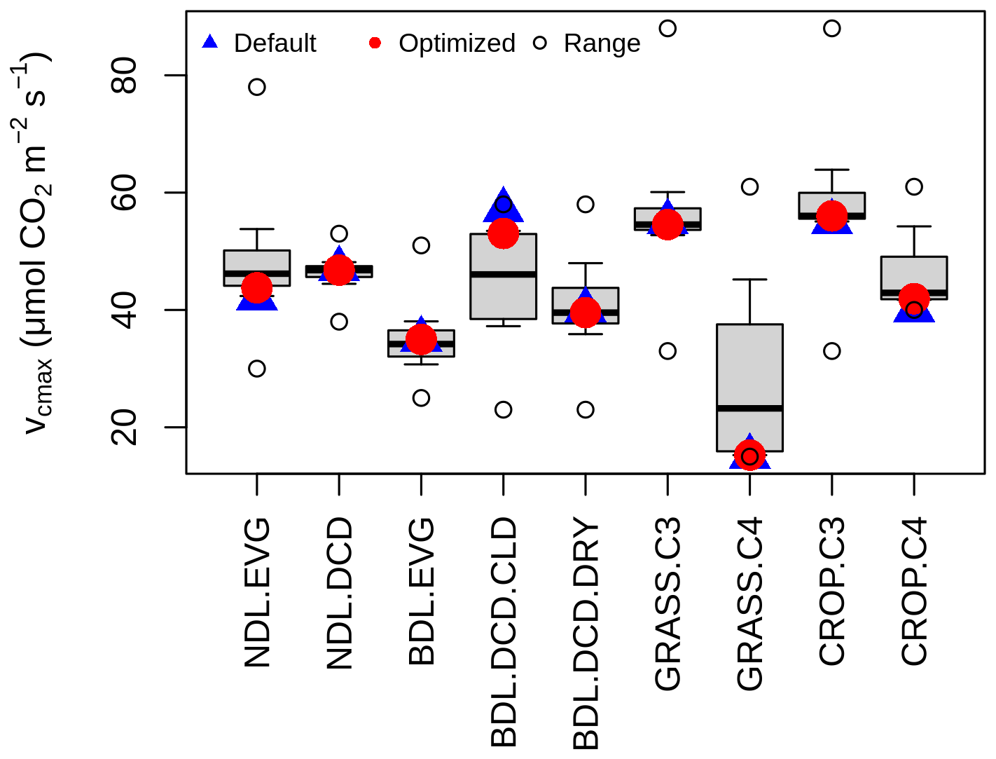
Figure 3 Synthetic data test when optimizing maximum carboxylation rate against modelled GPP for nine Plant Functional Types, namely needleleaf evergreen tree (NDL.EVG), needleleaf deciduous tree (NDL.DCD), broadleaf evergreen tree (BDL.EVG), broadleaf deciduous cold tree (BDL.DCD.CLD), broadleaf deciduous dry tree (BDL.DCD.DRY), C₃-photosynthesis grass (GRASS.C3), C₄-photosynthesis grass (GRASS.C4), C₃-photosynthesis crop (CROP.C3), and C₄-photosynthesis grass (CROP.C4). The boxplot displays the interquartile range, median, and 95th percentiles of the sampled parameter values, while the circles represent the full parameter uncertainty range.

3 Results

3.1 Optimization

As a first step, I assessed the effectiveness of the optimization through a synthetic data test. Rather than comparing the model output to global Earth observations, I compared it to model output generated with a known set of parameter values. If the optimization successfully recovers these known values, the process can be considered effective. The test was conducted using the nine default parameter values for the maximum carboxylation rate. Figure 3 demonstrates that the optimization accurately reproduces these parameter values, even when the true parameter values coincide with the minimum of the uncertainty range, as observed for C₄ grasses and C₄ crops.

Figure 4 AMBER scores per generation, where each generation consists of 100 chromosomes.

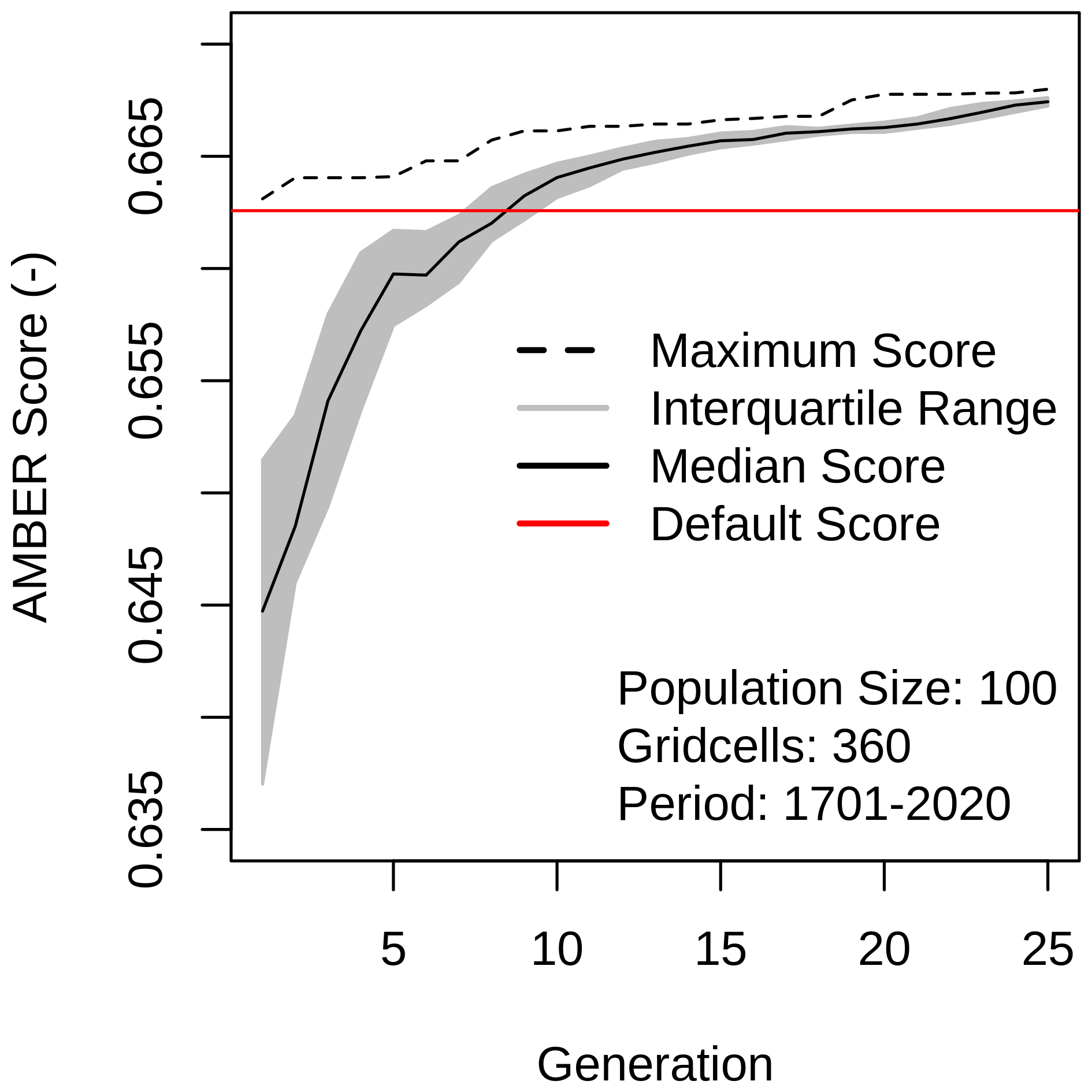
Next, I performed the optimization using all 28 parameters, which expand to 165 parameters when accounting for PFT-specific values, and 13 observation-based datasets. To enhance the efficiency of the optimization, the first chromosome of the initial generation contains the default parameter values. Figure 4 illustrates how the median AMBER score improves from generation to generation, surpassing the default score (denoted by the red line) that results from using default parameter values after approximately nine generations and levelling off after about 20 generations. The score spread among population members (grey-shaded area) decreases over generations until the interquartile range of the population almost matches that of the best-performing chromosome (stippled line), indicating that minimal improvement can be expected beyond 25 generations.

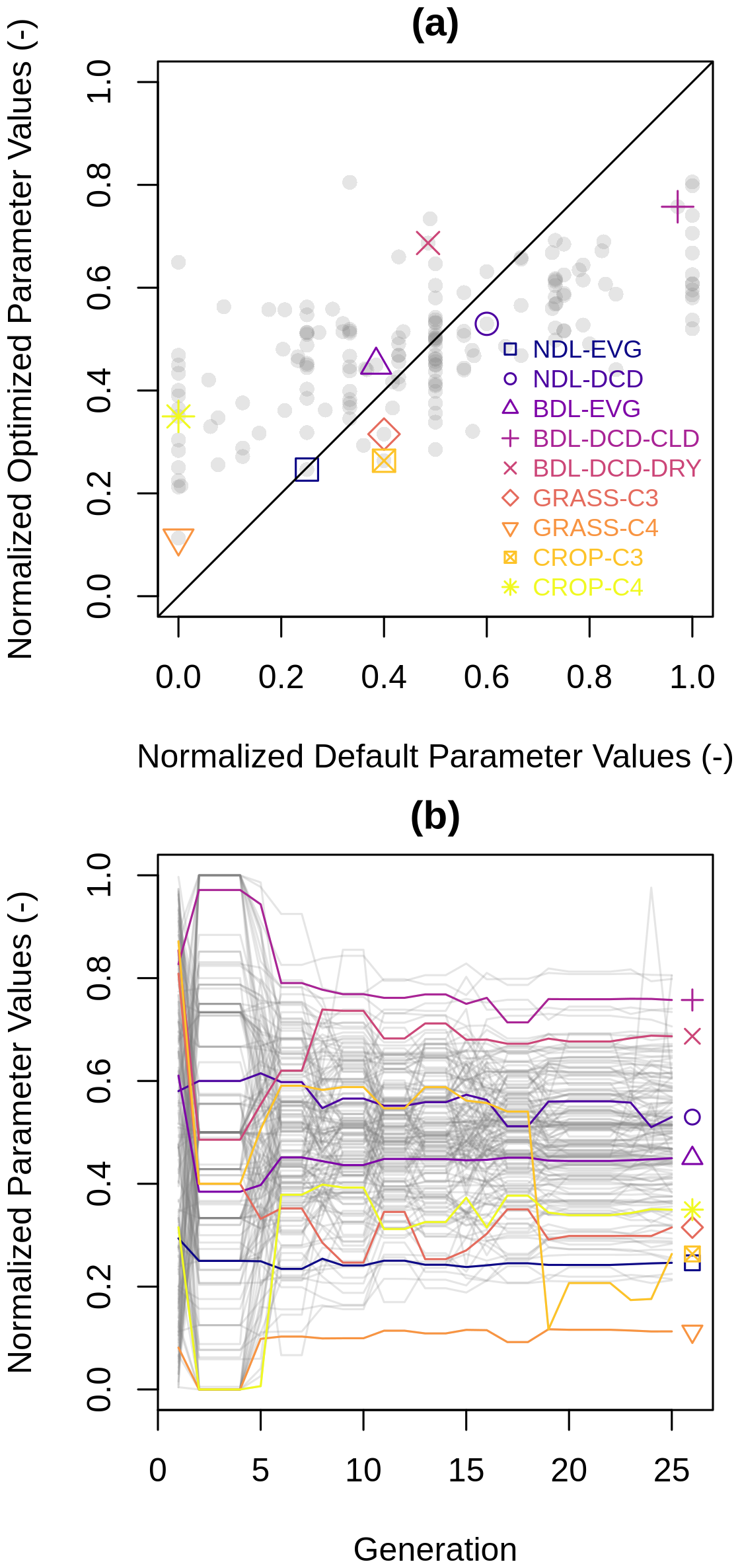
Figure 5 (a) Default versus optimized parameter values and (b) optimized parameter values of the chromosome with the highest fitness for a given generation. The coloured symbols and lines refer to the maximum carboxylation rate of nine plant functional types.

Comparing default against optimized parameter values shows that the optimization affected many parameter values, with differences of up to 60 % (Fig. 5a). For the maximum carboxylation rate, optimization increased the parameter values for some PFTs (e.g. broadleaf dry deciduous trees), left them unchanged (e.g. needleleaf evergreen trees) or decreased (e.g. broadleaf cold deciduous trees).

Figure 5b shows the normalized parameter values for the best-performing chromosome in each generation. The initial values on the left correspond to the default parameter settings, while the final values on the right represent the optimized values. Over the course of 25 generations, the parameter values of the best-performing chromosome changed multiple times, improving model performance with each adjustment. The optimized parameter values tend to cluster closer to the centre of the uncertainty ranges, with fewer values in proximity to the upper and lower limits. The next section explores equifinality using a Gaussian process emulator.

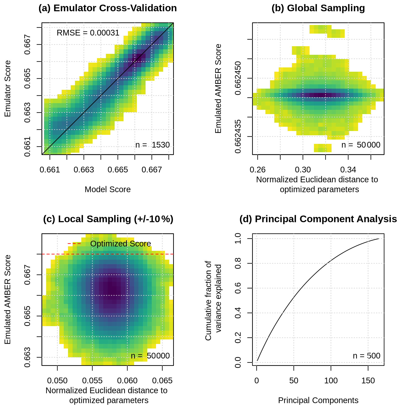
Figure 6 (a) Emulator cross-validation, emulated scores from 50 000 parameter value sets sampled (b) within each parameter's total uncertainty range and (c) within ±10 % of optimized parameter values, and (d) cumulative fraction of variance explained by principal components of emulated top 1 % performing parameter value sets. The colour scale indicates data point density, with darker colours showing higher densities.

3.2 Equifinality

This section explores equifinality using a Gaussian process emulator. To recall, the emulator was trained on a subset of the data produced during the optimization process (1530 simulations) and is used to estimate the AMBER score for a given set of parameter values. A comparison between the emulated and modelled performance scores obtained from cross-validation shows that the emulator accurately reproduces the model behaviour, with a root-mean-square error of 0.00031 (Fig. 6a). Next, I sampled the full uncertainty range of all 165 parameters using Latin hypercube sampling, generating 50 000 parameter sets and estimating the corresponding AMBER scores with the emulator. For each parameter set, I computed the Euclidean distance to the optimized parameter set, yielding one distance value per set. Plotting Euclidean distance against the emulated AMBER score shows that model performance remains nearly constant as distance increases, clustering around a score of 0.662 (Fig. 6b). This demonstrates that the model is subject to equifinality, as many distinct parameter combinations produce very similar score values. However, in all cases, the emulated AMBER score is lower than that of the optimized parameter set of 0.668.

To assess equifinality in regions of higher model performance, I generated a second ensemble of 50 000 samples by sampling within ±10 % of the optimized parameter values. Plotting Euclidean distance against the emulated AMBER score for this ensemble yields a circular cloud with a much wider range of scores than in the full-range sample (Fig. 6c). Notably, several parameter sets reach or even exceed the optimized score at a range of Euclidean distances. This further indicates that the model exhibits equifinality, even within regions of parameter space where performance exceeds the default score of 0.663.

Finally, I sampled within the parameter uncertainty ranges spanned by the top 10 % of parameter sets obtained during the optimization and used the emulator to generate a 5000-member ensemble. From this ensemble, I select the top 10 % of parameter sets and performed a principal component analysis to assess whether equifinality is driven by a few parameters or by many. Plotting the number of principal components against the cumulative fraction of variance explained shows that many principal components are required to explain most of the variance (Fig. 6c). This suggests that equifinality arises from the compensating effects of many parameters rather than a small subset.

To account for equifinality in the subsequent analysis, I selected the five best-performing parameter sets from the final ensemble used in the principal component analysis and ran CLASSIC with these parameter sets, first for the 360 grid cells and then globally. The mean emulated score of the five parameter sets closely matches the score obtained from the 360 grid cell CLASSIC simulations, with emulated and actual mean scores of 0.668 and 0.667, respectively. The next section evaluates CLASSIC performance when all land grid cells are forced with the optimized parameter sets. To account for equifinality, six parameter sets are used in total, including one obtained from the optimization and five identified by the emulator.

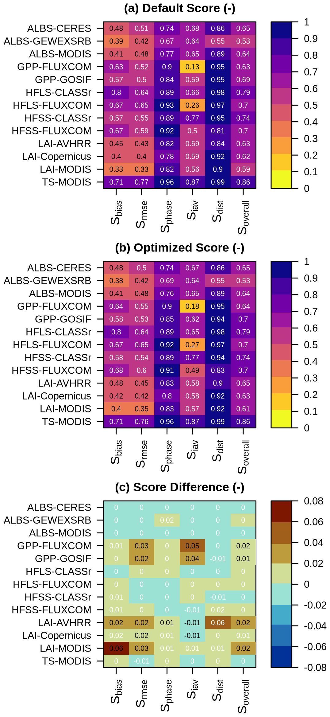
Figure 7 AMBER scores when running the model globally with (a) default and (b) optimized parameter values, with (c) presenting their differences. In (c), black numbers indicate statistically significant differences at the 5 % level.

3.3 Global Model Performance

Using the optimized parameter values obtained above, I conducted global simulations in which both the spinup and transient runs were based on six sets of optimized parameter values (one from the genetic algorithm and five from the emulator). The model outputs were compared against global Earth observations, and the resulting scores were evaluated against those from a simulation using the default parameter values. Focusing on the parameter set identified by the genetic algorithm shows that the optimization generally improves model performance for leaf area index and gross primary productivity, without causing any major deterioration in other variables (Fig. 7). The limited impact of the optimization on variables such as albedo and surface temperature was expected, as the optimized parameters predominantly influence carbon and turbulent heat fluxes, as discussed further in the Discussion section.

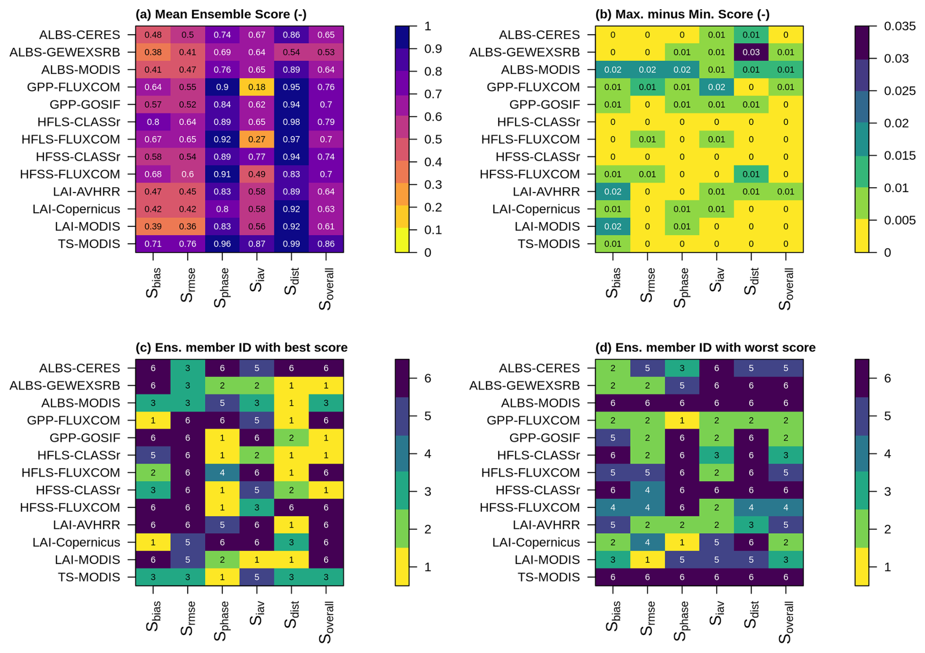
Figure 8 AMBER scores of an ensemble when running the model globally with optimized parameter values (ID = 1) and emulated (ID = 2–6) parameter values, where (a) is the mean score across all six ensemble members, (b) is the maximum minus the minimum score, (c) is the ensemble member ID with the best score, and (d) is the ensemble members with the worst score.

Assessing the performance of all six parameter sets together shows that the ensemble members perform very similarly (Fig. 8). Differences in model performance are most pronounced for albedo and leaf area index, but remain small, not exceeding 0.03. No ensemble member is consistently superior or inferior to the others. When counting the number of instances in which an ensemble member achieves the best overall score for a given variable, one parameter set identified by the emulator (ensemble member 6) outperforms the parameter set identified by the genetic algorithm (ensemble member 1).

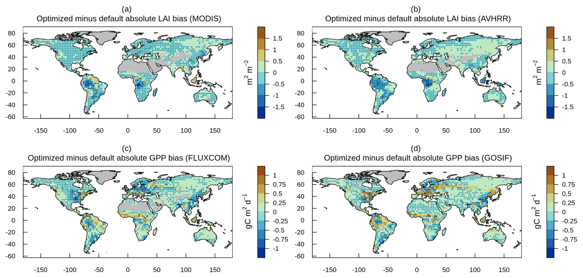
Figure 9 Optimized minus default absolute bias for leaf area index from (a) MODIS and (b) AVHRR, and for gross primary (c) FLUXCOM and (d) GOSIF, and sensible heat flux from (e) CLASSr and (f) FLUXCOM, where negative values imply bias reduction as denoted with black dots.

Figure 9 illustrates the difference between the optimized and default absolute biases for leaf area index and GPP, where negative values indicate a reduction in absolute bias due to optimization. Bias reduction is not confined to specific regions, but is evident across the vast majority of grid cells at all latitudes. For many grid cells, bias reduction reaches up to 1.5 m² m⁻² for leaf area index and 1 g C m⁻² d⁻¹ for GPP. One notable exception is Eastern Siberia, where bias reduction does not occur for either variable. In addition, bias reduction is more successful in the western than in the eastern Amazon.

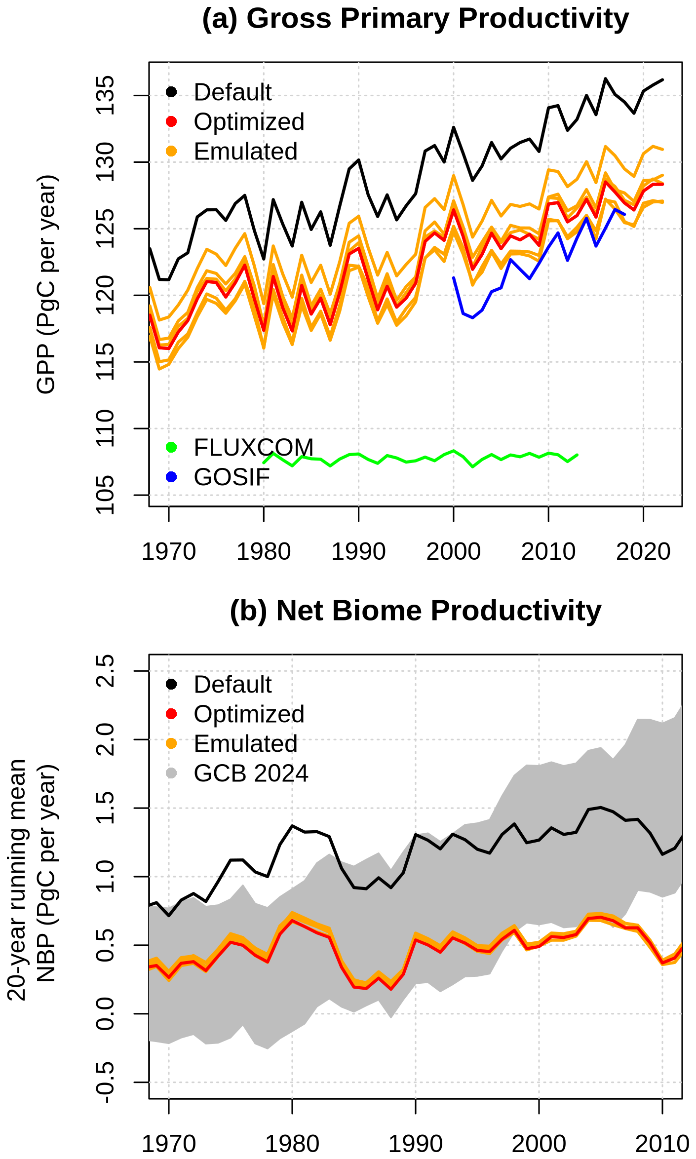
Figure 10 (a) Global gross primary productivity simulated by CLASSIC using the default parameter set (black), the optimized parameter set (red), and five parameter sets identified by the emulator (orange), together with the reference GPP data sets GOSIF and FLUXCOM. (b) Twenty-year running mean net biome productivity for the same CLASSIC simulations, compared with the reference NBP from GCB2024 (grey).

3.4 Global Carbon Fluxes

In this section, I evaluate how parameter optimization affects global GPP and NBP over recent decades. The optimization reduces global GPP by roughly 5 Pg C yr⁻¹, bringing the simulated values closer to estimates from the GOSIF reference dataset (Fig. 10a). The timing and magnitude of peaks and troughs in the time series are largely unaffected by the optimization. Simulations based on the emulated parameter sets form an ensemble that brackets the optimized run, with members producing both higher and lower GPP values (±2 Pg C yr⁻¹). In contrast, the FLUXCOM reference GPP is substantially lower than GOSIF (by about 15 Pg C yr⁻¹ in 2015) and exhibits a much weaker interannual variability and lacks a positive trend.

The default, optimized, and emulated parameter sets used in CLASSIC produce NBP values that, for most years, fall within the uncertainty range of the reference NBP from the Global Carbon Budget 2024 (GCB2024 NBP, hereafter) Friedlingstein et al. (2025) (Fig. 10b). The optimization reduces NBP by about 0.5 Pg C yr⁻¹ without affecting either interannual variability or the long-term trend. However, the simulated NBP does not reproduce the positive trend evident in GCB2024. Simulations using the emulated parameter sets yield NBP values that are nearly identical to those obtained with the optimized parameter set.

Table 3 Mean carbon fluxes (net biome productivity, gross primary productivity, autotrophic respiration, heterotrophic respiration, and emissions from fires) and pools (vegetation carbon and soil organic carbon) for CLASSIC simulations driven with default, optimized, and five different emulated parameter sets. The carbon fluxes and pools correspond to the last 20 years of the simulations, i.e. 2003–2022. Also given are the absolute and relative differences between simulations that are based on the optimized (opt) and default (def) parameter sets.

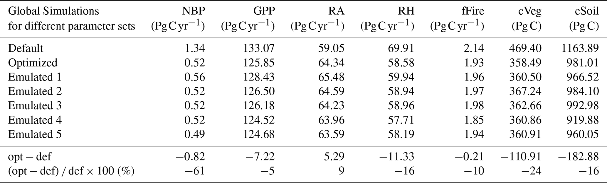
The optimization reduces global NBP over the period 2003–2022 by 0.82 Pg C yr⁻¹ (−61 %) (Table 3). This reduction is driven by a decrease in GPP (−7.22 Pg C yr⁻¹, −5 %) combined with an increase in autotrophic respiration (+5.29 Pg C yr⁻¹, +9 %). These effects are partially offset by a reduction in heterotrophic respiration (−11.33 Pg C yr⁻¹, −16 %). Carbon emissions associated with wildfires also decrease in response to the optimization, although their contribution is minor (−0.21 Pg C yr⁻¹, −10 %). Examining carbon stocks reveals that optimization decreases the vegetation carbon pool (−24 %), which aligns with the reduced GPP and increased autotrophic respiration. The decline in GPP also leads to a reduction in the soil organic carbon pool (−16 %), explaining the observed decrease in heterotrophic respiration. The impact of the emulated parameter sets is consistent with that of the optimized parameter set, although the exact values vary among simulations.

4 Discussion

This study demonstrates the effectiveness of optimizing poorly constrained land surface model parameters using machine learning and global Earth observations. The results show that optimization enhances model performance considerably, particularly for leaf area index and GPP. Using a prolonged optimization period (1701–2022), this improvement is achieved without the need to switch parameter values between the spinup and transient runs or the use of global scaling factors (Schürmann et al., 2016; MacBean et al., 2018). The Gaussian process emulator indicates that equifinality in the model is driven by compensating effects among many rather than few parameters. It also identifies alternative parameter sets that perform similarly well. Optimization reduces GPP by 5 % and increases autotrophic respiration by 9 %, resulting in a 61 % decrease in NBP compared with the default simulation over the 2003 to 2022 period. Alternative parameter sets identified by the emulator produce similar outcomes, with global GPP uncertainty in 2022 spanning roughly 4 Pg C yr⁻¹. The following paragraphs explore these results in greater detail, discuss the study's limitations, and highlight opportunities for future research. Furthermore, I will argue that advanced methods of regular parameter tuning should become an integral part of the model development cycle. Finally, I will examine the broader implications of this research for climate change policy.

While the optimization clearly improved global GPP when evaluated against GOSIF reference data, this did not yield an obvious improvement in global NBP when evaluated against GCB2024 NBP (Friedlingstein et al., 2025). In particular, neither the default nor the optimized simulations reproduce the GCB2024 NBP trend. One way to improve simulated global NBP would be to optimize CLASSIC parameters using the GCB2024 NBP estimates as a target. However, this would require running the model for all grid cells during the optimization process, which is computationally prohibitive. A feasible alternative would be to conduct the global optimization using an emulator. This would require generating a training dataset based on global CLASSIC simulations, with parameter values sampled randomly across their respective uncertainty ranges. Once trained, the emulator could first be used to perform a global sensitivity analysis to identify the most influential parameters and then to optimize those parameters.

One aspect not addressed in this study is the sensitivity of the results to the choice of optimization strategy, including the selection, crossover, and mutation operators, as well as their associated hyperparameters. Different combinations of these components may yield more efficient convergence or lead to different optimized parameter sets. However, systematically tuning the optimization itself is challenging due to the high computational cost. Although alternative settings could be tested using shorter simulations or fewer grid cells, it is unclear whether such results would generalize to the full optimization setup. Future research could therefore explore more efficient ways of identifying effective optimization strategies, for example by using an emulator to guide the design and tuning of the optimization procedure.

The impacts of optimization vary across different variables. The most significant improvements are observed in leaf area index and GPP. In contrast, no noticeable changes in performance are detected for albedo and land surface temperature. This outcome aligns with the selection of parameters being tuned, which were chosen based on a global sensitivity analysis that identified the most influential parameters for carbon and turbulent heat fluxes (Deepak et al., 2025). Including additional variables in the optimization helps ensure that the enhancements in carbon and heat fluxes do not compromise model performance elsewhere. However, improving albedo and land surface temperature would require a broader or different selection of parameters.

Optimization leads to a reduction in carbon stocks, raising the question of whether the optimized values remain consistent with observations. Global datasets synthesizing empirical measurements vary considerably, with reported ranges spanning from 264.6 to 482.5 Pg C for vegetation carbon and 1143.4 to 2708.0 Pg C for soil organic carbon (Seiler et al., 2022). The optimized vegetation carbon is 358 Pg C, which falls within this range. However, the optimized soil organic carbon (981 Pg C) is lower than the reported range. This study did not include carbon stocks as target datasets in the optimization process due to the large uncertainties in these products. Moreover, comparing modelled carbon stocks with reference data requires additional processing, including extracting the top 1.5 m soil layers and distinguishing above-ground from below-ground biomass to align model outputs with observations. This adds to the already substantial computational burden, as this processing must be repeated for each of the 2500 simulations. However, future optimization efforts could assess how incorporating carbon stocks as constraints affects the optimization outcomes. Global reference data used for land surface model evaluation are subject to considerable uncertainties (Seiler et al., 2022). Many data assimilation frameworks treat observational uncertainty in a more formal manner than is presented here, commonly by specifying error covariance matrices for both model and observational errors (Tarantola, 2005). These covariance matrices determine how strongly observations constrain the model and help avoid overfitting in regions or periods of large uncertainty. However, estimating error covariance matrices reliably remains challenging, particularly in the absence of comprehensive uncertainty documentation for many Earth observation products (MacBean et al., 2022). The approach presented in this study is intentionally simpler. All observational data products are given equal weight, and no explicit assumptions are made about their error magnitudes or spatiotemporal error correlations. For example, consider two satellite-based GPP products. If both products indicate lower GPP than the model, the optimization will adjust parameters such that the modelled GPP is reduced. If, however, one product indicates higher and the other lower GPP, the performance score remains similar as long as the modelled GPP lies within the range spanned by the two products. In this sense, the approach implicitly downweights conflicting information and avoids tuning the model toward any single potentially biased product. While this procedure does not explicitly model observational error covariances, it achieves a similar practical outcome by reducing sensitivity to individual datasets and by preventing overfitting in the presence of observational disagreement. Importantly, it avoids introducing additional assumptions about poorly constrained error structures. Moreover, whereas covariance-based data assimilation primarily focuses on minimizing instantaneous model-data mismatch, the approach adopted here explicitly constrains multiple statistical properties of the system, including bias, centralized RMSE, seasonal timing, interannual variability, and spatial correlation (the five AMBER scores). Improvements in these higher-order diagnostics are not guaranteed through bias correction alone and therefore benefit from being constrained explicitly.

The CLASSIC configuration used in the present study prescribes the maximum carboxylation rate. Alternatively, the model can calculate the maximum carboxylation rate based on the dynamic interaction between the carbon and nitrogen cycles. The nitrogen cycle is particularly important for accounting for the modulating effect of nitrogen limitation on the CO₂ fertilization effect (Thornton et al., 2007). In the case of CLASSIC, the nitrogen cycle leads to a weaker carbon sink that absorbs about 50 % less carbon between 2015 and the end of this century under SSP5-8.5 (Kou-Giesbrecht and Arora, 2022). Past research has shown that model performance deteriorates considerably when the model's nitrogen cycle is activated (Arora et al., 2023). The large uncertainty of nitrogen cycle parameters presents an opportunity to refine them using the parameter optimization system introduced here.

The results demonstrate that parameter optimization has a strong influence on net carbon fluxes, aligning with previous studies that have reported even more pronounced changes in terms of net ecosystem exchange or NBP (Peylin et al., 2016; Schürmann et al., 2016; Bacour et al., 2023). The magnitude of this impact is comparable to adding a new process to the model. The large impact of parameter optimization on net carbon fluxes presents a compelling argument for modelling groups to incorporate advanced optimization methods into their model development cycle. However, it must be noted that model tuning can be a double-edged sword. On one hand, optimization ensures that the model performs as well as possible for the given parameter uncertainty ranges. This reduces the likelihood that mismatches between model output and observations are due to parameter uncertainty, making it easier to identify issues such as coding errors, poor process representation, or missing processes. On the other hand, optimization can mask deficiencies by compensating for model limitations, potentially making the model appear more accurate than it actually is and complicating efforts to diagnose problems. However, these challenges are not unique to automated optimization, they also apply to traditional manual tuning. When a model developer incorporates a new process, they typically adjust parameter values to align the model output with reference data, which can similarly obscure underlying deficiencies. Moreover, as models evolve, parameter values that were previously selected may no longer be the most appropriate. For these reasons, adopting more advanced parameter optimization techniques in the model development cycle is a logical and necessary step toward improving model accuracy and reliability.

The model configuration used here is an offline simulation with prescribed [CO₂] and meteorological forcing. Therefore, the impacts of optimization do not alter atmospheric [CO₂] or the climate. In a fully coupled simulation, lower NBP would imply a faster increase in [CO₂] and temperature, affecting NBP in return. This feedback could be evaluated in an emissions-driven simulation where CLASSIC runs within CanESM and the carbon cycle is fully coupled. Such simulations would not only be scientifically relevant but also important for global climate change mitigation policy, as explained next.

The goal of the 2015 Paris Agreement is to limit the warming of global mean surface temperature to well below 2 °C and preferably 1.5 °C compared to pre-industrial values (Horowitz, 2016). The remaining carbon budget that is consistent with the 1.5 °C global warming target is estimated at 200 Pg CO₂ (55 Pg C) for the year 2024 (>50 % chance) (Forster et al., 2024). Current CO₂ emissions are about 40 Pg CO₂ yr⁻¹. If emissions remain at present levels, we will likely exhaust the remaining carbon budget consistent with the 1.5 °C warming target by the end of this decade.

The remaining carbon budget is calculated using the Model for the Assessment of Greenhouse Gas Induced Climate Change (MAGICC) emulator (Meinshausen et al., 2011). MAGICC is a simple carbon cycle-climate model with a hemispherically averaged upwelling-diffusion ocean coupled to an atmospheric layer and a globally averaged carbon cycle model. Version 7.0 is calibrated against ESMs, such as CanESM5, which are part of the Coupled Climate-Carbon Cycle Model Intercomparison Project (C4MIP) (Jones et al., 2016; Meinshausen et al., 2020). Any advancements in CanESM could therefore improve future estimates of the remaining carbon budget and, consequently, influence climate change mitigation policy. This further strengthens the case for adopting more advanced methods of parameter optimization.

5 Conclusions

In conclusion, this study demonstrates the effectiveness of optimizing poorly constrained land surface model parameters using machine learning and global Earth observations. The optimization improves model performance considerably for leaf area index and GPP. While the model exhibits high-dimensional equifinality, the simulated carbon fluxes remain robust across alternative parameter sets with similar model performance. The optimization weakens the terrestrial carbon sink, underscoring the need to explicitly address parameter uncertainty in order to reduce inter-model differences. Although parameter tuning was conducted in an offline mode, the optimized parameter sets could be applied in online, emission-driven simulations in which the carbon cycle is fully coupled. To enhance model accuracy and reliability, modelling groups should integrate advanced parameter optimization methods into their development cycle. Doing so will not only improve model performance but also support more robust climate change mitigation policies.

Appendix A: Model Evaluation

Global NBP is estimated as the difference between fossil fuel emissions (E_FOS) and the atmospheric growth rate (G_ATM), the ocean sink (S_OCEAN), and the cement carbonation sink (S_CEMENT), all of which are available from 1960 onwards:

$$\begin{array}{}\text{(A1)}& \text{NBP}=E_{\mathrm{FOS}}-G_{\mathrm{ATM}}-S_{\mathrm{OCEAN}}-S_{\mathrm{CEMENT}}.\end{array}$$

Friedlingstein et al. (2025) provide not only the annual values of each term but also the corresponding uncertainty ranges, expressed in terms of standard deviation (σ), for all terms except S_CEMENT. Using uncertainty propagation, I estimate the uncertainty of global NBP as follows:

$$\begin{array}{}\text{(A2)}& {\mathit{\sigma }}_{\mathrm{NBP}}={\left({\mathit{\sigma }}_{E_{\mathrm{FOS}}}^{\mathrm{2}}+{\mathit{\sigma }}_{G_{\mathrm{ATM}}}^{\mathrm{2}}+{\mathit{\sigma }}_{S_{\mathrm{OCEAN}}}^{\mathrm{2}}\right)}^{\mathrm{0.5}}.\end{array}$$

Appendix B: Equifinality

The normalized Euclidean distance $\widehat{d}$ to the optimized parameter values is defined as:

$$\begin{array}{}\text{(B1)}& \widehat{d}={\displaystyle \frac{\sqrt{{\sum }_{i=\mathrm{1}}^p({\mathit{\theta }}_i-{\mathit{\theta }}_i^{*}{)}^{\mathrm{2}}}}{\sqrt{p}}},\end{array}$$

where ${\mathit{\theta }}_i^{*}$ is the set of optimized parameter values, θ_i is a set of sampled parameter values, and p is the number of parameters.

Appendix C: Gaussian process emulator

The following provides a numerical example that illustrates how a Gaussian process emulator works. We use the squared exponential (RBF) kernel with variance σ²=1 and length scale ℓ=1:

$$\begin{array}{}\text{(C1)}& k(x,x^{\prime })={\mathit{\sigma }}^{\mathrm{2}}\exp \left(-{\displaystyle \frac{(x-x^{\prime }{)}^{\mathrm{2}}}{\mathrm{2}{\mathrm{\ell }}^{\mathrm{2}}}}\right).\end{array}$$

We are given training inputs x and training outputs f:

$$\begin{array}{}\text{(C2)}& \mathit{x}=\left[\begin{array}{c}\mathrm{0.0}\\ \mathrm{1.0}\end{array}\right],\mathit{f}=\left[\begin{array}{c}\mathrm{3}\\ \mathrm{5}\end{array}\right].\end{array}$$

The test input is $x_{*}=\mathrm{0.75}$. Using the kernel function above with ℓ=1.0 and σ²=1.0, the covariance matrix with nugget term is:

$$\begin{array}{}\text{(C3)}& {\mathbf{K}}_y=\left[\begin{array}{cc}\mathrm{1.0000010}& \mathrm{0.6065307}\\ \mathrm{0.6065307}& \mathrm{1.0000010}\end{array}\right].\end{array}$$

The cross-covariance matrix ${\mathbf{K}}_{*}=k(\mathbf{x},{\mathbf{x}}_{*})$ is:

$$\begin{array}{}\text{(C4)}& {\mathbf{K}}_{*}=\left[\begin{array}{c}\mathrm{0.7548396}\\ \mathrm{0.9692332}\end{array}\right].\end{array}$$

The test covariance matrix is:

$$\begin{array}{}\text{(C5)}& {\mathbf{K}}_{**}=\left[\mathrm{1}\right].\end{array}$$

The inverse covariance matrix is:

$$\begin{array}{}\text{(C6)}& {\mathbf{K}}_y^{-\mathrm{1}}=\left[\begin{array}{cc}\mathrm{1.5819733}& -\mathrm{0.9595143}\\ -\mathrm{0.9595143}& \mathrm{1.5819733}\end{array}\right].\end{array}$$

The predictive mean is therefore:

$$\begin{array}{}\text{(C7)}& {\mathit{\mu }}_{*}={{\mathbf{K}}_{*}}^{\top }{\mathbf{K}}^{-\mathrm{1}}\mathbf{f}=\mathrm{4.837537},\end{array}$$

and the predictive covariance is:

$$\begin{array}{}\text{(C8)}& {\mathrm{\Sigma }}_{*}={\mathbf{K}}_{**}-{{\mathbf{K}}_{*}}^{\top }{\mathbf{K}}^{-\mathrm{1}}{\mathbf{K}}_{*}=\mathrm{0.0164838}.\end{array}$$