Projected elevation-dependent warming in the Alps: contrasting free-atmosphere and surface trends with surface energy balance drivers

Because of topography, climate change exhibits complex regional imprints in the Alps. This study aims at understanding the processes that link elevation-dependent warming (EDW) – i.e. the modulation of temperature trends with elevation – at seasonal scale in the Alps with the surface energy balance. We investigate projected EDW patterns in the Alps using 7 km resolution simulations spanning the period 1961–2100 made with the Modèle Atmosphérique Régional (MAR), exploring scenarios SSP2-4.5 and SSP5-8.5 and driven by two general circulation models, EC-Earth3 and MPI-ESM1-2-HR. We find a larger yearly warming signal at high elevations (1.2 to 1.5 °C °C⁻¹ of global warming) than at low elevations (1.1 to 1.3 °C °C⁻¹ of global warming), with contrasted seasonal patterns and intensities (up to 2 °C °C⁻¹ of global warming at high elevations in summer). EDW profiles are found to be different near the surface than in the free atmosphere. Near the surface, a maximum warming is found in spring at mid-elevations that is migrating to higher elevations in summer and autumn. This signal is not found in the free atmosphere. The elevation of the maximum warming is moving upward, consistently with the snowline migration over the years in a warming climate. Investigating surface energy balance trends reveals a link between the profiles of EDW and those of net shortwave radiation and energy used to melt snow. The snow-albedo feedback linked to the net shortwave radiation trend is found to be responsible for two thirds of the impact of the snowline on warming, while snow melt accounts for the last third. Melting limits the warming at high elevation when snow is persisting. We suggest that snow melting is an important driver of EDW that should be considered in any EDW-snow investigations.

1 Introduction

Mountain regions face singular challenges with climate change due to their topography. They are hotspots of biodiversity thanks to their often unique ecosystems which are vulnerable to rapid climate change (Rahbek et al., 2019). They host large water resources for both local and remote inhabitants (Viviroli et al., 2020), in relation to both orographic precipitation and snow and glacier melting, which can make downstream inhabitants eventually vulnerable to climate change further up the slopes (e.g. Colombo et al., 2023). Their orography influences the atmospheric circulation at the synoptic scale, through local variation of the atmospheric flow and at the hemispheric scale through planetary waves triggered by the mountains, extending their influence to the surrounding regions.

Climate change in the mountains shows specific features, in particular because of potential Elevation-Dependent Warming (EDW). EDW is defined as the modulation with elevation of near-surface atmospheric temperature trends, a warming “along the slopes”. Although it is sometimes simplified as a linear regression of warming against elevation (e.g. Rangwala et al., 2010; Tudoroiu et al., 2016; Palazzi et al., 2017; Palazzi et al., 2019; Toledo et al., 2022), studies increasingly show nonlinearity in the dependency of warming with elevation (e.g. Kotlarski et al., 2012, 2015, 2023; Palazzi et al., 2017; Minder et al., 2018; Beaumet et al., 2021; Toledo et al., 2022; Napoli et al., 2023). Indeed, the drivers of EDW are numerous, interconnected, and may be confined to certain elevations. Hence, EDW profiles are highly variable depending on the area and the period considered (Ohmura, 2012, Pepin et al., 2025). Pepin et al. (2015) give an overview of different processes that may impact EDW (albedo, clouds, water vapour, blackbody emission and aerosols) and the shape of their expected elevational dependency. EDW has been investigated in different mountainous areas: in the Alps (see reviews by Gobiet et al., 2014; Kuhn and Olefs, 2020); in High Mountain Asia, where small EDW signals have been reported over the last decades (Li et al., 2020) but are expected to intensify in future projections (Dimri et al., 2020). A strong EDW is simulated in the Rocky Mountains and is linked to the snow-albedo feedback (Minder et al., 2018). Contrasted EDWs are suggested for minimum and maximum daily temperature in the Andes, in relation with shortwave and longwave radiation changes (Toledo et al., 2022) or specifically reduced cloudiness and snow (Chimborazo et al., 2022). In places where it has a strong seasonal cycle, snow is identified as one of the major drivers of EDW through the snow-albedo feedback (Rangwala et al., 2010; Kotlarski et al., 2015, 2023; Minder et al., 2018; Palazzi et al., 2019; Warscher et al., 2019; Beaumet et al., 2021; Byrne et al., 2024).

The Greater Alpine Region (GAR) is one of the most studied mountain regions in the world. Observation data broadly point towards an enhanced warming at high elevations in this region (Pepin et al., 2022), but an opposite signal can be found depending on the area and the period of interest (Philipona, 2013; Tudoroiu et al., 2016; Rottler et al., 2019). Overall, EDW in the GAR is not yet fully characterized and understood. This is mainly due to limitations in the amount of high-elevation observations on the one hand, and model grid resolutions that are coarse with respect to the orography on the other hand.

Simulations made with General Circulation Models (GCMs) are able to reach finer and finer resolutions as computational resources increase, but are still falling short of adequately representing the complex topography in mountain regions (Sandu et al., 2019) and in the Alps in particular when studying climate change and its drivers (Palazzi et al., 2019). The need arises then to downscale these products to more suitable resolutions. Regional Climate Models (RCMs) are a frequently-used method to dynamically downscale GCMs. They allow for simulations at∼ 10 km scale resolution, ensuring a better representation of the topography and the mountain climate, as well as explicitly representing several physical processes that have to be parameterised at coarser resolutions.

As mentioned earlier, snow is a crucial driver of EDW, making it an important variable to represent correctly in simulations used to study climate change in mountain regions. A finer model resolution improves the representation of snow (Lüthi et al., 2019), but even the 12 km resolution of the EURO-CORDEX experiments yields significant biases (Terzago et al., 2017; Matiu et al., 2020), highlighting the need for even finer resolutions. Most RCMs also have a simple representation of the snowpack, using a single layer varying in thickness over time. In our study, we use 7 km resolution experiments made with the Modèle Atmosphérique Régional (MAR, Gallée and Schayes, 1994), a RCM further described in the next section, that uses a detailed multi-layer snow cover scheme.

MAR simulations at 7 km forced by the ERA-20C reanalysis (ECMWF Reanalysis of the 20th century; Poli et al., 2016) have been performed previously to investigate the past evolution of climate and EDW in the Alps (Beaumet et al., 2021). The results highlight seasonal contrasts in EDW over the period 1959–2010, with larger warming found at low elevations in winter (< 1000 m a.s.l.), at high elevations in summer (> 2000 m a.s.l.) and at intermediate elevations in spring (1500–1800 m a.s.l.). In this study, we aim to investigate the simulated EDW in the Alps from 1961 to 2100, considering different future projections following the scenarios SSP2-4.5 and SSP5-8.5 (from 2015 to 2100). In order to investigate the processes driving EDW, we focus on all the components of the surface energy balance. To our knowledge, this is the first study where all these components are analysed, in addition to using 140-years-long simulations until the end of the century at a high resolution.

First, the data and methods are described in Sect. 2. We delve into the results in Sect. 3 by: (i) exploring the warming footprints in the Alps in our simulations; (ii) comparing EDW profiles near the surface and in the free atmosphere; (iii) investigating trends in the surface energy balance components and (iv) determining the elevation changes of the snowline and of the other drivers affecting the temperature trend. A discussion and a conclusion are offered in Sect. 4.

2 Data and methods

2.1 Model data

2.1.1 The Modèle Atmosphérique Régional (MAR)

MAR is a hydrostatic, primitive equation, limited-area model with constant sigma coordinates on the vertical axis (Gallée and Schayes, 1994; Gallée et al., 2005). It has been developed for polar regions (e.g. Fettweis et al., 2017, Agosta et al., 2019, Amory et al., 2021) and mountainous environments (e.g. Ménégoz et al., 2013 over the Himalayas; Ménégoz et al., 2020; Beaumet et al., 2021 over the Alps; Collao Barrios (2018) in Patagonia; Fettweis et al., 2023 in the Vosges mountain region). This wide range of applications is supported by its comprehensive multi-layer snow cover scheme (Brun et al., 1992) which accounts for the laws of metamorphism in the snow, allowing to simulate accurately the evolution of the snow cover stratigraphy. It has also been used over western Africa (Kouassi et al., 2010, Chagnaud et al., 2020) to study the tropical hydrological cycle.

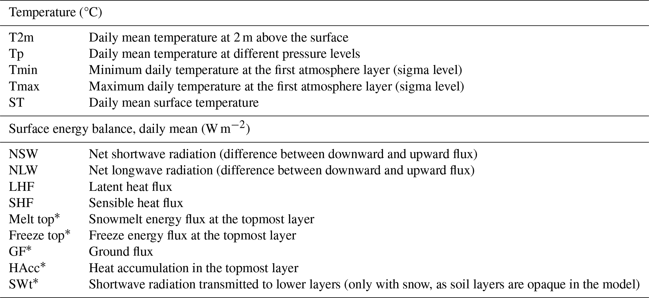
In the present work, data from simulations using two successive versions of MAR, 3.10 and 3.14, are analysed. Simulations made with version 3.10 were indeed missing some of the surface energy balance components as diagnostic variables (see Table 1). A new simulation using the latest version of MAR, version 3.14, was thus run in which all the variables of interest were saved. Using both versions' simulations allows us to increase the spread of investigated scenarios and climate sensitivities that we explore.

MAR version 3.10 uses a radiative transfer scheme developed by Morcrette (1991, 2002) and used in the ERA-40 reanalyses (Uppala et al., 2005). Owing to some identified issues within MAR of this scheme with downward radiation (e.g. Delhasse et al., 2020), and its lack of modularity, the Morcrette scheme has been replaced by the ecRad radiation scheme (Hogan and Bozzo, 2018) in version 3.14 of MAR (Grailet, 2023). The second difference between the two versions of MAR for the present paper lies in the climatology of aerosols. In version 3.10 aerosols have a yearly climatology that evolves until 2005 – later years use the 2005 climatology. Version 3.14 by contrast uses the climatology provided by the European Center for Medium Range Weather Forecasts (ECMWF, cycle 43r3 – see Bozzo et al., 2020) which remains fixed throughout the whole simulation.

2.1.2 The simulations over the Alps

MAR is applied over the Alps at a 7 km resolution. This resolution was chosen to depict the alpine topography – with its narrow valleys and snow-covered peaks - more accurately than the 12.5 km EUROCORDEX resolution while still being compatible with the hydrostatic approximation in middle latitudes configurations (which imposes a∼ 5–10 km resolution at the lowest). This resolution smoothes the Alps to a maximum elevation close to 3400 m a.s.l. – compared to under 3000 m a.s.l. in 12.5 km EUROCORDEX simulations – while the real maximum elevation is 4808 m a.s.l. at Mont Blanc. Within the Alps, most elevations are around the 1000–1200 m a.s.l. range at this resolution (Fig. 1b). The domain extends from 1.5 to 18.5° E and from 41.5 to 49.5° N (Fig. 1a).

Table 1 MAR variables used in this study. Variables with a ^* are only available for the MAR version 3.14 simulation.

Due to human and computational constraints, a large ensemble approach exploring model and scenario variability was not pursued. Instead, a storyline-based approach was adopted, relying on a limited-area model that accurately simulates the relevant physical processes. From the CMIP6 database (Eyring et al., 2016), we retained for our study the two GCMs showing the best skill over the European-North-Atlantic area (80° W–45° E, 35–75° N): EC-Earth3 and MPI-ESM1-2-HR. This choice is based on a comparison with the ERA5 reanalysis over 1971–2000, using the weighted mean square error of 3 variables: the temperature at 700 hPa, the geopotential height at 500 hPa, and the sea surface temperature weighted at half weight (see Eq. A1 in Appendix A). These variables were selected to evaluate the skill of the GCMs to reproduce the large scale climate features, as the RCM is expected to represent the smaller scale processes. Table A1 (Appendix A) summarises the results of this evaluation. The selected criteria and forcing GCMs are consistent with the recommendations detailed in Sobolowski et al. (2025): the geopotential height at 500 hPa criterion ensures an appropriate large-scale atmospheric circulation, the sea surface temperature a realistic oceanic forcing, and the temperature at 700 hPa allows to discriminate GCMs that would provide too high biases in the middle troposphere. As Sobolowski et al. (2025), we highlighted MPI-ESM1-2-HR and EC-Earth3 as two GCMs exhibiting an appropriate level of skill for climate downscaling over Europe (see Table 2 therein).

CMIP6 simulations include a historical period available over 1850–2014 and future projections over 2015–2100, based on different scenarios, including in particular the intermediate greenhouse gas emissions (SSP2-4.5) and the high emission scenario SSP5-8.5 (O'Neill et al., 2016). In this study, we use the following four 1961–2100 simulations made with either version 3.10 or version 3.14 of MAR:

• MAR version 3.10 forced by EC-Earth3 (historical, 1961–2014; SSP2-4.5, 2015–2100);

• MAR version 3.10 forced by MPI-ESM1-2-HR (historical, 1961–2014; SSP2-4.5, 2015–2100; SSP5-8.5, 2015–2100);

• MAR version 3.14 forced by MPI-ESM1-2-HR (historical, 1961–2014; SSP5-8.5, 2015–2100).

Hereafter, the simulations will be referred to as MAR-EC-Earth3 SSP2, MAR-MPI SSP2, MAR-MPI SSP5, and MARv3.14-MPI SSP5 respectively.

The v3.10 MPI simulations have previously been presented in Bacer et al. (2024). We include here the v3.10 MAR-EC-Earth3 SSP2 and MARv3.14-MPI SSP5 simulations.

We present the variables (and associated acronyms) used in this study in Table 1.

The outputs of MAR are described in Appendix B, along with the surface energy balance in the soil and snow routine in MAR (see Fig. B1 for an illustration of the routine).

A data set for a limited number of variables and levels is available online (see “Data availability” at the end of this paper).

Beaumet et al. (2021) find biases in temperature and snow cover in the Alps in MAR simulations forced by reanalyses (ERA-20C and ERA5) when comparing to gridded observational datasets, reanalyses and in-situ observations. In their study, the MAR experiments are found to slightly overestimate temperature at low elevations and underestimate at high elevations, especially in winter. They also are found to underestimate snow cover duration at low elevation (< 1500 m a.s.l.). Nevertheless, the biases found are typical of RCMs and are overall considered acceptable.

By comparing the MAR simulations used in the present study to gridded observational datasets based on station interpolation (see Appendix C, Figs. C1–C4), these simulations were found to have a cold bias reaching maximum values up to 3 °C at high elevations (above ∼ 2000 m a.s.l.) across the seasons and a generally warm bias at lower elevations (below 1000–1500 m a.s.l. depending on the season), especially in summer for which it can reach maximum values of 4 °C. There is also a wet bias in precipitation at high elevation (above 1500 m a.s.l., except in summer which has a dry bias) reaching around 7 mm per day in winter. Lower elevations (below ∼ 1000 m a.s.l.) tend to have a dry bias (∼ 2 mm on average, up to 5 mm) in summer and autumn. Also, compared to satellite estimates (Appendix C, Fig. C5), MAR shows a too long snow cover duration at high elevations (above ∼ 2000 m a.s.l.) for all seasons (a bias reaching maximum values of 50 additional days of snow in spring and summer), and a too small amount of snow days at low elevations (below ∼ 1000 m a.s.l.) in winter (up to 40 fewer days of snow). The biases provided here are an estimation, since observational datasets over the Alps also have large uncertainties (a problem typically found in all mountain regions), due in particular to the inherent missing values in such products (Prein and Gobiet, 2017; Kotlarski et al., 2019; Matiu et al., 2024) that are not discussed in this article.

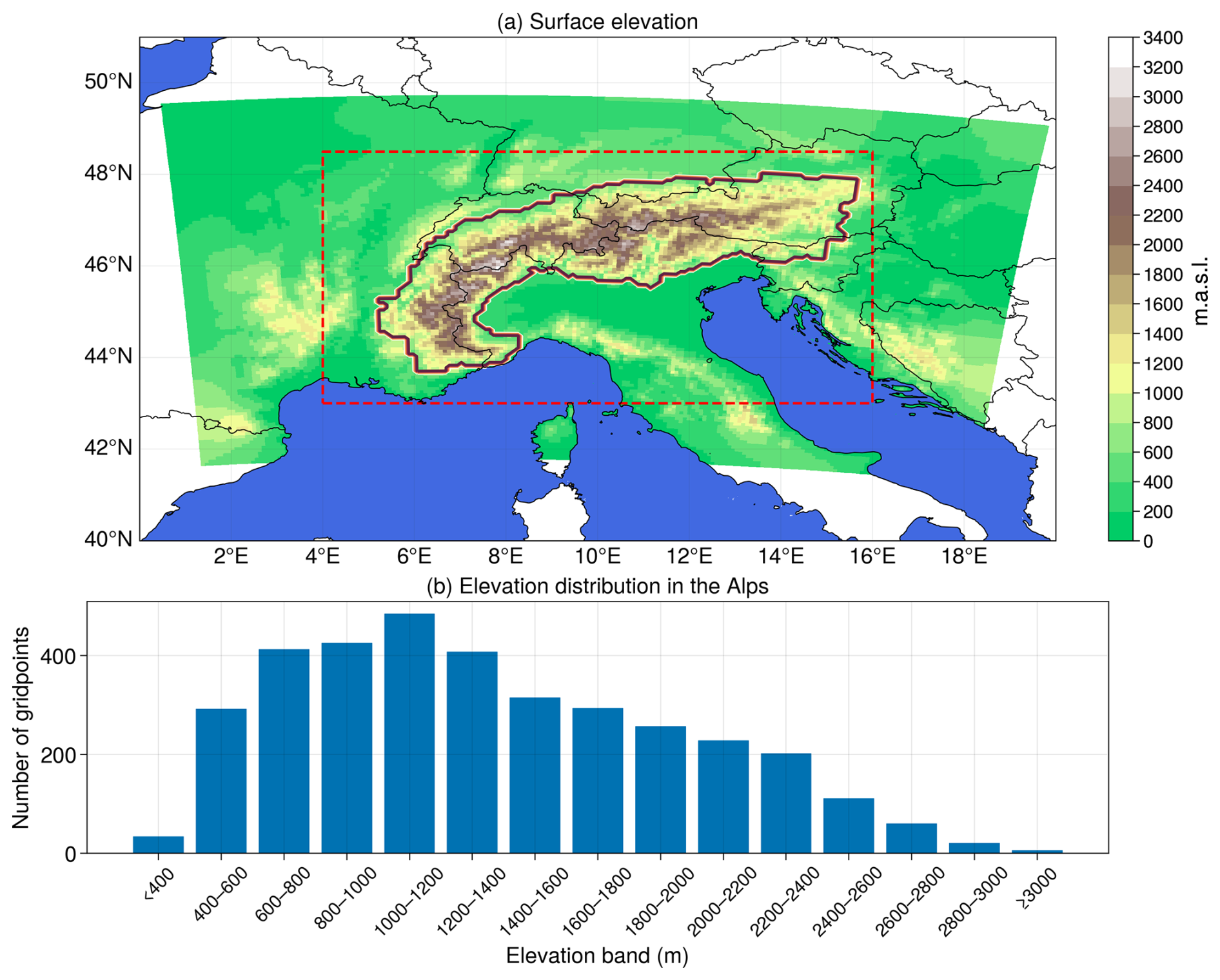
Figure 1 (a) Domain and orography of MAR simulations. The contour defines the Alps (see Sect. 2.2.2) and is used as a mask further on in this paper (e.g. whenever there is a value averaged over the Alps). The red box is the area shown in Fig. 2, corresponding to the domain considered after excluding the lateral parts affected by boundary conditions in the MAR experiments. (b) Distribution of elevation inside the alpine contour discretized over 200 m elevation bands. There are six gridpoints lying above 3000 m a.s.l.

2.2 Methods

2.2.1 MAR warming as a function of global warming

As a preliminary step before studying EDW, we produce the maps of MAR warming as a function of global warming. For this, we combine all three v3.10 simulations (excluding the v3.14 simulation to avoid giving too much weight to the same model-scenario pair).

We first compute the global warming in each GCM forcing simulation by averaging yearly as well as spatially the global monthly 2 m air temperature from 1850–2100. We then fit a 3rd degree B-spline using 4 kn through the resulting series of 251 yearly global temperature. This allows us to have a smooth correspondence between any given year and the global mean temperature in the forcing simulation (see Appendix D). We choose 1961–1990 as a reference period to compute the warming anomaly (subtracting the mean of the reference period to the global mean temperature spline). We regress at each gridpoint the three merged MAR v3.10 anomalies onto the global warming level given by the splines. This allows us to get an estimation of the local warming as a function of global warming. Finally, we apply the same procedure at the seasonal scales.

2.2.2 Elevation-dependent trends in the Alps

In this study, we consider historical and projected trends for temperature and surface energy balance fluxes. The historical period spans 1961–2014 and the projection 2015–2100. For each grid point, period and variable of Table 1, we compute the trend in the seasonal mean with a linear regression against the years.

In order to consider elevation-dependent trends at the scale of the Alps, we first apply a mask to our data to isolate the Alps, by selecting the grid points that satisfy the two conditions of being at least 360 m above sea level (m a.s.l.) and having a neighbouring grid point at 1300 m a.s.l. or more (see the contours in Figs. 1 and 2). These criteria were tested and selected to accurately trace the contour of the Alps while excluding other mountain areas present in the simulated domain.

Then, we classify the grid points into 200 m-elevation bins and compute the mean and standard deviation of the trends for each bin, for any given variable. The temperature in the free atmosphere is the only variable that is not classified in bins, as it is available at seven different pressure levels in the MAR v3.10 outputs (five in version 3.14).

2.2.3 Elevation change of maximum trends

In order to track the evolution of the elevation of the maximum trend (defined below) at intermediate to high elevations in temperature and surface energy balance fluxes, we first smooth the seasonal data at each grid point by fitting a 3rd degree spline with the year as covariate (implemented with an adaptive smoothing parameter s used to choose the number of knots, $s=N\times v$ with N the number of years and v the variance of the yearly series), in order to remove the year-to-year noise. Then, we divide the 1961–2100 simulation into 90 overlapping 50-year windows (1961–2010, 1962–2011, …, 2051–2100) and compute the difference between the first and last year of the estimated spline at each grid point and for each window. At this point we have one trend per grid point and window.

Then, for each window, we fit another 3rd degree B-spline using 5 kn through the scatter plot of grid point trends versus the elevation. We take the elevation of the maximum warming after excluding the lowest 10 % and highest 0.3 % elevations of the spline to properly target the local maximum at intermediate elevations in windows that feature a global maximum at the bottom or the top of the elevation range (see Appendix E). For each variable, we end up with an elevation of maximum trend for each window, and thus with a temporal evolution of the elevation of maximum trend.

2.2.4 Snowline elevation

The snowline elevation can be computed with different methods, and three of them are provided here: we compute over the Alps and for each day (i) the mean elevation of the 10 highest grid points having < 1 millimeter water-equivalent (mmWe) of snow, (ii) the mean elevation of the 10 lowest grid points having ≥ 1 mmWe of snow, and finally (iii) the average of these two criteria. The first criterion gives an estimate of the elevation above which all grid points have snow, the second criterion the elevation below which no grid points have snow. The two elevations define a snow transition band between them, in which some grid points have snow and some don't.

We then take the seasonal median of these daily values to get an average of the snow line elevation over the whole period or window.

3 Results

3.1 Warming footprint in the Alps

See Fig. 1 for the definition of the contour line. Isolines every 1000 m are shown.

Figure 2 shows the yearly and seasonal warmings in the three v3.10 MAR simulations with respect to global warming (see Sect. 2.2.1). As seen in Fig. 2a, yearly temperatures are rising faster at higher elevations in the Alps (∼ 1.2 to 1.5 °C °C⁻¹) than in the surrounding lowlands, which are already warming at a faster rate than global warming (∼ 1.1 to 1.3 °C °C⁻¹). There is also a strong longitudinal gradient in this area, the continental climate in the Eastern part warming faster than the Western European climate that is under an oceanic influence.

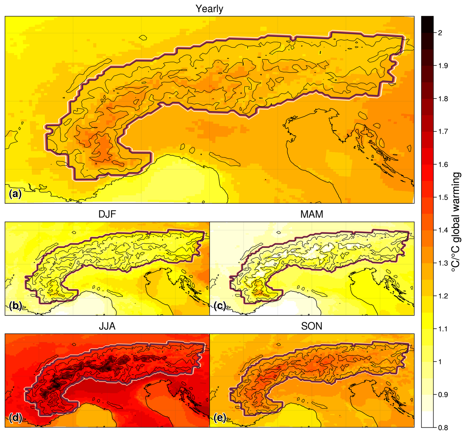
Figure 2 (a) Yearly warming over 1961–2100 in the three v3.10 simulations scaled with respect to global warming level in the forcing GCM. (b), (c), (d), (e): same as (a) at the seasonal timescale.

Overall, strong seasonal contrasts can be seen both in warming intensity and pattern over the Alps (Fig. 2b, c, d, e).

The warming is particularly intense in summer (JJA) with values around 1.6 to 1.7 °C °C⁻¹ global warming in the lowlands, and reaching twice the global warming at high elevations. In contrast, the domain warms at a similar rate to global warming (1–1.1 °C °C⁻¹) in spring (MAM) and at even lower rates (0.8–0.9 °C °C⁻¹) at high elevation, except in the southern Alps. Autumn (SON) is similar but less extreme than summer, while winter (DJF) is similar to spring, albeit showing a slightly higher warming rate.

The pattern of warming is opposite between summer and spring: summer shows the highest rates of warming at high elevations, where spring shows its lowest rates of warming. The exception being in the southern Alps, where this pattern is reversed.

It is therefore essential to consider seasonal timescales in order to understand the processes that are behind these contrasting patterns.

3.2 Elevation-dependent warming near the surface and in the free atmosphere

Figure 3 shows the temperature trend at 2 m above the surface and in the free atmosphere (at different pressure levels) at the scale of the Alps, for the four simulations over the historical (1961–2014) and the projection (2015–2100) periods, using the method of Sect. 2.2.2.

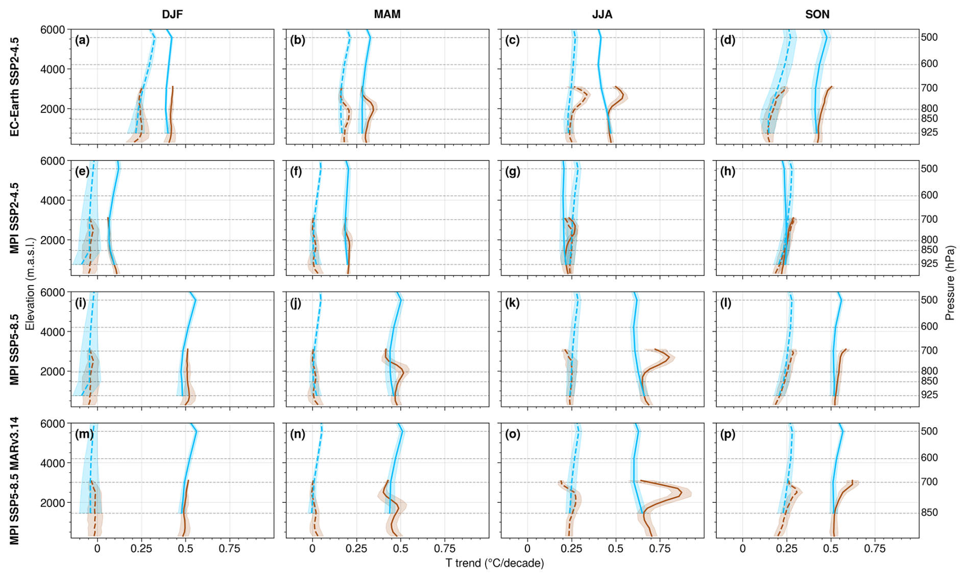
Figure 3 Alpine temperature trends near the surface (along the slopes) averaged over 200 m-elevation bins (T2m, brown) and in the free atmosphere averaged over the available pressure levels (Tp, blue). The historical period (1961–2014) is in dashed lines, projection (2015–2100) is in full lines. Shaded bands represent the spatial standard deviation (1σ). The first three rows are based on the MAR v3.10 simulations and the last one on the MAR v3.14 experiment. Columns are for each season.

Overall, the warming is generally larger in the projection than in the historical period, both in the free atmosphere and near the surface. The exception is in summer and autumn for the MAR-MPI SSP2 simulation (Fig. 3g and h) where the two periods experience similar warming. The lowest temperature trend is close to zero in winter in the historical period for the MPI simulations (Fig. 3e, i and m). The largest warming is simulated in summer with the MARv3.14-MPI SSP5 simulation (Fig. 3o) and reaches 0.86 °C per decade on average at 2500 m a.s.l., i.e. almost 7.4 °C of warming between 2015 and 2100.

Looking at their vertical profiles, the rates of warming in the free atmosphere and near the surface have a similar altitudinal gradient in winter. The trend values are similar, with slightly larger trends for the near-surface warming and a larger spatial standard deviation.

In spring, the same can be generally said for the low and high elevations. However, we can see higher rates of warming at mid-elevations near the surface than in the free atmosphere for both periods in MAR-EC-Earth3 SSP2 (Fig. 3b), and for the projection periods of MAR-MPI SSP5 (Fig. 3j and n).

For MAR-EC-Earth3 SSP2, in spring, the maximum of warming near the surface is found at a higher elevation in the projection than in the historical period, suggesting an upwards migration of the underlying cause for this heightened near-surface warming.

In summer and autumn, the near surface maximum warming signal moves at higher elevations, with the strongest signal seen in summer for MARv3.14-MPI SSP5 (Fig. 3o).

This enhanced surface warming appearing at mid-elevations in spring, moving upwards and increasing in summer, and continuing to move upwards with a lower intensity in autumn, is investigated along with its link to surface processes in the next section.

In some simulations and periods, we also see a rate of warming lower near the surface than in the free troposphere that is located above the elevation of the maximum warming. This can particularly be seen in the SSP5 simulations in spring for the projection (Fig. 3j, n) and in summer for the historical period (Fig. 3k, o).

In the free atmosphere, the warming is generally more skewed towards lower (925 hPa) and higher (500 hPa) elevations in the projection period than in the historical period (see panels a, c, d, e, i, j, k, l, m, o, p of Fig. 3). This leads to some altitudinal trends having a hook shape, further discussed below (see Sect. 4). The warming in the free atmosphere in the MAR experiment is following very closely the warming simulated in the forcing GCMs, especially at high elevations (not shown). This highlights low atmosphere and surface feedbacks simulated with MAR that cannot be solved by the GCMs whereas the regional climate is driven by large-scale features of the GCM projections.

In the continuation of this study, we investigate this seasonal signal occurring near the surface by analysing the surface energy balance fluxes and their respective trends.

3.3 Projected temperature and energy flux trends

We define the surface energy balance in the model MAR as the sum of all fluxes occurring at the first surface layer of the ground and of the processes occurring within that layer – heat accumulation, snow melt and water refreezing. In this model, the first surface layer of the ground is 1 mm thick in the absence of snow and has the (variable) depth of the first snow layer in the presence of snow. The surface energy balance is expected to be closed, meaning that the sum of the fluxes is expected to be equal to zero.

By identifying all the variables that are part of this balance (see Sect. 2.1) and computing their trends, we ensure that we have a comprehensive view of what is happening at the surface and that we do not overlook any process contributing to increased surface warming. Only MARv3.14 results are used here as this version allows to display all the different energy fluxes. The two versions have similar EDW trends in the Alps as displayed by the last two rows in Fig. 3.

Figure 4 displays the profiles along the elevation of the projected mean values and trends for temperatures and surface energy fluxes. The blue horizontal lines indicate the mean elevation of the snowline for each season using the method presented in Sect. 2.2.4. The top and bottom lines can be seen as a snow transition band including the snow line.

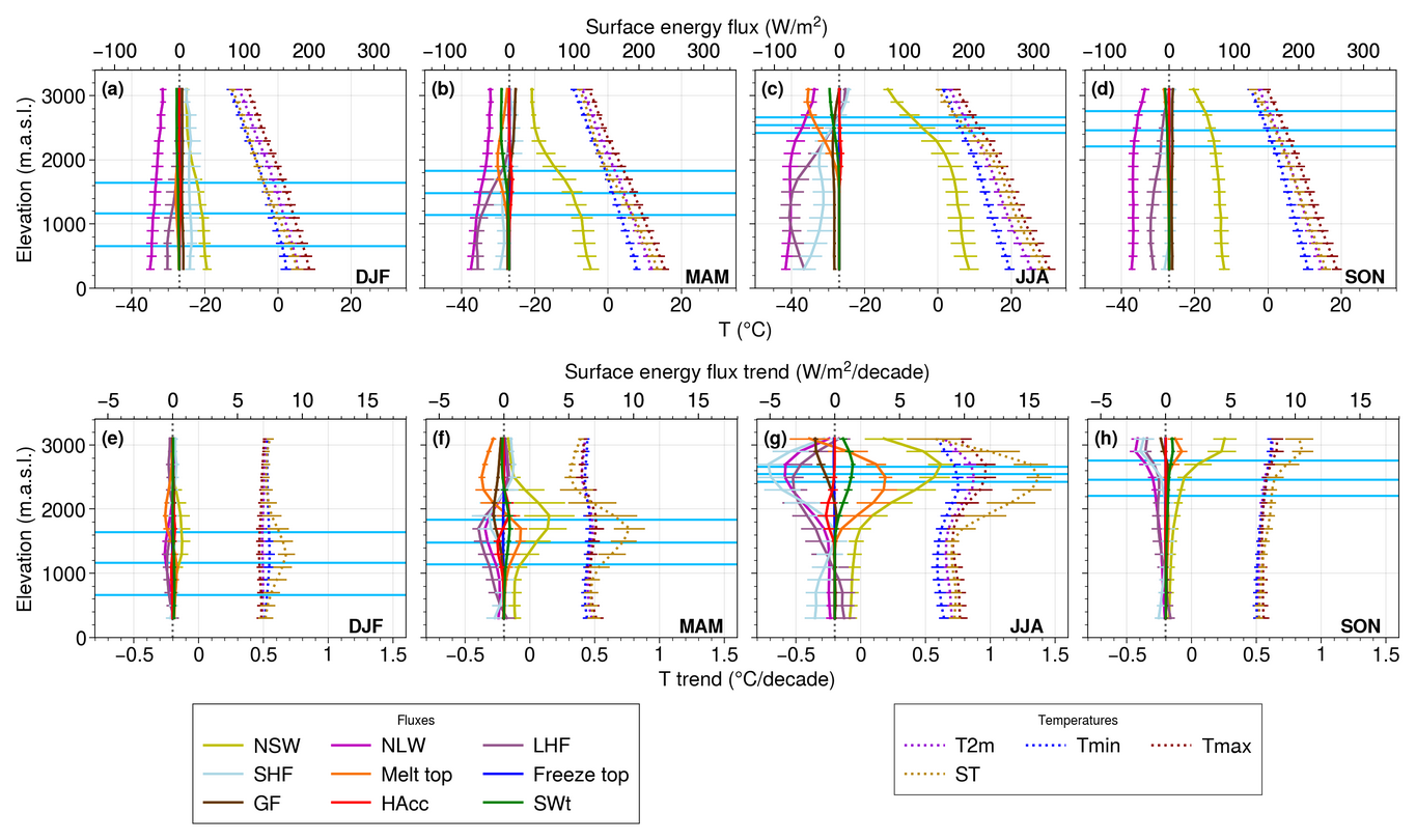
Figure 4 Profiles along the elevation of the projected (2015–2100) mean values (top) and trends (bottom) for temperatures (dotted) and fluxes (full lines) averaged over the Alps, in the MAR v3.14 simulation. For each panel, the temperature (trend) values are indicated on the lower axis and the surface energy flux (trend) values on the upper axis. Horizontal bars are the spatial dispersion (1 sigma). Blue horizontal lines refer to the elevation of the snowline computed in three different ways (cf. Sect. 2.2.4). Fluxes are positive when directed towards the surface. Season is indicated in the bottom right corner.

The average values (top row) highlight the sign and the vertical distribution of the temperature and surface energy fluxes. Fluxes are defined as positive when directed towards the surface. The mean NSW flux is positive for all seasons with a seasonal cycle that reaches its maximum in summer, as expected, and decays with height. A stronger decay above the snowline showcases the impact of the presence of snow on the NSW flux. The mean NLW flux is the main component balancing the NSW flux, and as such has a similar profile except that it is negative and follows a weaker seasonal cycle. The SWt flux is negative in the presence of snow, since it is being transmitted to the lower layers from the surface, and equal to zero in the absence of snow since the ground is opaque in the model.

The mean LHF is negative (except at the top), meaning that evaporation is cooling down the surface (humidity transfer from the surface to the atmosphere). It decreases with height as well – which might be due to less available NSW flux at high elevations – except at the bottom in summer (Fig. 4c), which might be due to less available humidity at low elevations. The mean SHF is positive in winter, indicating that the surface is being heated up by turbulent fluxes in the surface boundary layer (ST is cooler than T2m). It is negative at low elevations in spring, summer, and autumn, as ST is warmer than T2m, and switches sign at higher elevations. Mean melt top is always negative by convention (energy is used by the surface to melt snow) and largest in summer. It is larger at intermediate elevations in winter and spring, because temperature is too low to induce melting at high elevation, and larger near the top of the profile in summer and autumn. We do not delve into the other variables because of their low amplitude.

The bottom row of Fig. 4 shows that T2m, Tmin and Tmax exhibit similar trends, while ST exhibits the largest trend, near the top of the snow band. This suggests again that the maximum T2m trends are mainly driven by surface processes. The closer to the surface, the stronger the temperature trend signal. The surface absorbs more energy over time which is then redistributed to the near-surface atmosphere thanks to the longwave radiation and sensible and latent heat fluxes, explaining the temperature signal found close to the surface that shows a similar shape but with a smaller intensity.

In spring and summer, ST also exhibits a minimum trend at higher elevations.

Let us remember that a positive trend means an increase for a positive flux, but a decrease for a negative flux. NSW and NLW fluxes both show a clear increase in their absolute values over time and throughout the seasons, which is expected in a warming climate. By contrast, SWt is decreasing, which is explained by the decrease in snow cover over time.

LHF and SHF have large trends that generally point to an absolute increase, but not for all elevations, as both the mean values and the trends switch signs at different elevations and seasons. They might be in part a response to the perturbations in NSW flux and melting.

GF, HAcc and Freeze have small or non-existent trends.

Melting flux shows large trends in spring and summer. For both seasons, the trend first increases with elevation, then decreases until it ends as a negative trend near the top of the elevational gradient. As seen with the temperature, the melt trend is larger and shifted to higher elevations in summer compared to spring, as expected. The presence of both a maximum trend, and then a minimum trend at higher elevations, is reminiscent of the surface temperature trend and the lower rate of warming above the maximum signal discussed in the previous section.

Figure 4 shows evidence that the snow-albedo feedback is the main driver of the elevation-dependent warming signal. Indeed, the NSW variable shows the largest trend at the snow transition band elevations. The NLW, SHF and LHF trends compensate for this increase to maintain the surface energy balance with a maximum trend at similar elevations but negative in sign.

Melting strongly impacts the surface energy balance and temperature as well, with a positive trend within the snow transition band, transitioning to a negative trend above. The snow melt energy flux is negative (top row of Fig. 4) which means that the snow melt increase (negative trend) is slowing down the warming at elevations where there are still significant amounts of snow, and the snow melt decrease (positive trend) is speeding up the warming where snow is becoming scarce. This is due to the phase transition from solid to liquid water. When the snowpack reaches 0 °C, additional energy provided by e.g. solar radiation is consumed to melt the snow without an increase in temperature in the system. Once the snowpack is no longer present, the energy which was used to melt the snow is back to increasing the surface temperature once again.

In spring, the mean trend of the snow melt energy flux reaches a maximum of 1.31 W m⁻² per decade and a minimum of −1.71 W m⁻² per decade along the elevation profile, while the mean NSW trend reaches a maximum of 3.50 W m⁻² per decade. Assuming that the difference between the warming at low elevations and at the snowline is mainly due to snow-related processes, we can subtract the former to the latter to get a first order approximation of the effect of the snowline on the two variables. This assumes that (i) snow-related processes are minimal or non-existent at low elevations, and (ii) that the signal is otherwise independent of elevation which is de facto the case for snow melt, and reasonable to assume for the NSW trend given that the treeline is fixed in the model. With this approximation, the NSW trend is closer to 2.63 W m⁻² per decade and the melt to 1.27 and −1.75 W m⁻² per decade.

In summer, the mean trend of the snowmelt energy flux reaches a maximum of 3.90 W m⁻² per decade and a minimum of −1.96 W m⁻² per decade, while the NSW trend reaches a maximum of 8.18 W m⁻² per decade. Subtracting the trend at low elevations to approximate at the first order the effect of the snowline alone, the NSW trend is closer to 7.12 W m⁻² per decade (melt is unchanged).

For both seasons, the NSW maximum trend is slightly more than twice the snow melt energy flux trend (either positive or negative). This means that while the snow-albedo feedback effect is the main cause behind the simulated elevation-dependent warming in both seasons, the snow melt change is also having a significant effect on the warming at and near the surface.

The snowline is expected to migrate upwards with global warming. In the continuation of this study, we investigate if there is a similar migration in the elevations of the maximum trends.

3.4 Snowline and elevation of maximum warming

Figure 5 shows the evolution of the elevation of the maximum trend throughout the MARv3.14-MPI SSP5 simulation spanning 1961–2100 for T2m, ST, Tmax, NSW and the melt flux for rolling 50-year windows (see Sect. 2.2.3). Superimposed is the elevation of the snowline using the criteria defined in Sect. 2.2.4 for each 50-year window.

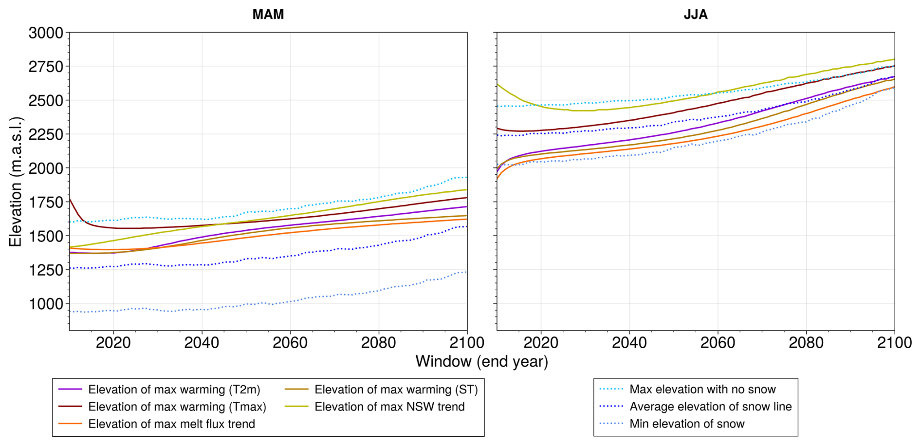
Figure 5 Elevation of snowline, maximum warming trends (T2m, Tmax, ST), melt flux trend and net shortwave trend in spring and summer over the course of rolling 50-year windows spanning 1961–2100 in the MAR v3.14 simulation over the Alps. The final year of each window is shown on the x axis.

In spring, the snow transition band migrates by approximately 300 m to higher elevations between the first (1961–2010) and the last (2051–2100) windows. The elevations of the maximum trends are contained within this band and shift similarly, with shifts ranging from 200 m to over 400 m (not counting the first few windows for Tmax where the maximum trend is higher than expected).

In summer, the snow transition band is narrowing and migrates to upper elevations. The top of the band increases in elevation by approximately 300 m between the first and last windows, the bottom by approximately 550 m. The elevations of the maximum trends are again mostly contained within this band. They migrate upwards by 450 to 650 m, except for NSW which is unexpectedly high and decreasing in elevation for the first 10–15 windows.

This suggests a correlation between the migration of the snow transition band and the elevation of maximum warming, the latter staying largely contained within the former in spring and summer in the span of the entire simulation.

4 Discussion and conclusion

In this study, we analysed four MAR simulations over the Greater Alpine Region in order to investigate the physical drivers of EDW. We saw higher warming in the Alps compared to the global warming simulated in the forcing GCMs: 1.2–1.5 °C °C⁻¹ at the yearly timescale. The warming reaches higher values in summer, with values around 1.7 °C °C⁻¹ at low elevations and up to 2 °C °C⁻¹ at the highest elevations. We found a reversed EDW in spring, with a warming at high elevation that reaches lower values than the global warming (0.8–0.9 °C °C⁻¹). The different warming patterns from season to season highlighted the need to investigate EDW at the seasonal timescale. Then, we compared the warming near the surface (along the slopes) and in the free atmosphere and highlighted a maximum signal along the slopes moving upwards from spring to summer to autumn. This local warming is explained by surface-atmosphere exchanges, since it does not happen in the free atmosphere. There is no clear EDW in winter, which could be explained by a lower available amount of solar radiation, making temperature trends less dependent on its variations at the surface. Among the different surface energy fluxes, NSW and melt energy fluxes have a maximum trend at a similar elevation than the maximum temperature trend, located near the top of the snow transition band (i.e. where the snow starts to disappear in a warming climate). Assuming the signal seen at the elevation of the snowline is mainly due to these two snow-related processes, almost two thirds of this maximum warming is explained by NSW changes (2.63 W m⁻² per decade in spring, 7.12 W m⁻² per decade in summer), whereas melting changes contribute over a third in our model experiments (−1.75 to 1.27 W m⁻² per decade in spring, −1.96 to 3.90 W m⁻² per decade in summer). Finally, we saw that the trends of T2m, Tmax, ST, NSW and melting fluxes show a maximum value at an elevation that moves upward over time. This happens at the elevation of the snow transition band, i.e. in the elevation band covering the areas where the snow cover starts to disappear and where the last snow patches are remaining.

An added value of the simulations used in this study compared to previous studies on EDW in the Alps with model data (Kotlarski et al., 2012, 2015, 2023; Gobiet et al., 2014; Palazzi et al., 2019; Lüthi et al., 2019; Warscher et al., 2019; Beaumet et al., 2021; Napoli et al., 2023) is the combination of (i) a fine resolution at 7 km; and (ii) a large timespan of 140 years covering both historical and projection periods. The 7 km resolution allows for a good compromise between the representation of the alpine orography (to reduce snow cover biases seen e.g. at 12 km in the EURO-CORDEX experiments; see Terzago et al., 2017; Matiu et al., 2020) and the hydrostatic approximation required in MAR experiments. The large timespan allows for investigating trends in a context where natural variability induces small signal-to-noise ratios.

Pepin and Seidel (2005) find enhanced warming at the surface compared to the free atmosphere in global mountain regions by comparing surface temperature in observation data sets and free atmosphere temperature from an interpolated reanalysis product for the period 1948–1998. However, the weakest signal in absolute value is found for locations over Europe (see Table 4 within). In the Rocky Mountains, Minder et al. (2018) find stronger warming rates along the slopes than in the free troposphere in RCM experiments, highlighting the role of the snow-albedo feedback. To our knowledge, our study is the first one that is providing a similar finding in the Alps, with a complete view of all the surface processes at play.

The melting of snow consumes energy due to the phase transition of snow to liquid water. This process limits the warming above the snowline at elevations where melt is increasing, and enhances the warming below the snowline where melt is decreasing. As stressed above, with the aforementioned assumptions in mind, we find that it is responsible for approximately a third of the snowline's impact (positive or negative) on warming in the MAR version 3.14 simulation. We suggest that this process is a driver of EDW and should be considered in any EDW-snow investigations.

The impact of snow on elevation-dependent warming is often simplified to the snow-albedo feedback effect (e.g. Pepin et al., 2015; Palazzi et al., 2019; Warscher et al., 2019; Byrne et al., 2024). Thornton et al. (2021) identify snow melt as an essential mountain climate variable, but from a hydrological standpoint only. Dimri et al. (2022) investigate snow melt trend as a function of elevation in the Indian Himalayan region, seeing a similar signal to ours: the snow melt trend transitions from positive (the melting process decreases over time) to negative (that process increases) when going from low elevations to high elevations. The signs of the trends are reversed in their study as they look at the snow melt in kg m⁻², which is positive, while the present study looks at the melt contribution to the surface energy balance, which is negative. However, they do not mention a possible contribution of the energy consumed by snow melt, again only mentioning the effect on albedo. Minder et al. (2018) find, when removing the snow-albedo feedback, similar EDW profiles between the free troposphere and near the surface. However a small signal near the surface remains in their study. We may hypothesize this to be the melt energy flux in light of our study.

Our study is based on a small ensemble experiment (two configurations with two different forcing GCMs, one of them with two scenarios) due to resource constraints preventing us from producing and exploring a larger ensemble. We use a single RCM, which has its own climate sensitivity (Glaude et al., 2024). As seen in Appendix C (Fig. C5), the MAR simulations used in this study tend to overestimate the duration of snowcover on the ground, mainly due to an overestimation of precipitation at high elevations. This might exaggerate the impact of snow on EDW. Larger ensemble experiments would help to diagnose the temperature and snow changes, disentangling the forced signals versus those related to climate internal variability. Nevertheless, it is useful to identify the patterns and the physical drivers of EDW with single experiments, since ensemble averaged signals might overwhelm the local enhanced trends that might differ among GCM-RCM configurations.

This study utilized a simplified framework to isolate and study specific processes. Two main prospects for further characterization of EDW in the Alps appear in our model framework: (i) we are considering a fixed aerosol climatology in our future projections (stationary forcing over 2005–2100 in version 3.10 and over the entire period in version 3.14), that is limited to the aerosol direct effect (indirect effects are neglected). This prevents the possibility of investigating the local cooling related to particle pollution that is mainly active at the bottom of the valley (Napoli et al., 2022) and that is currently decreasing in Europe with a significant impact on surface temperature (Philipona, 2013; Tudoroiu et al., 2016; Nabat et al., 2025). (ii) The model also uses a stationary land surface cover which excludes the possible effect of the migration of the tree line on EDW. These two aspects should be investigated in future work.

Further research could also investigate other processes acting as feedback on EDW. An increase in humidity (i.e. atmospheric moisture) entails an increase in the downward longwave radiation, and the Planck feedback entails an increase in the upward longwave radiation. Moreover, seasonal contrasts may be reinforced due to these processes: in winter, humidity is higher than in summer and temperature is lower, potentially strengthening one process over the other in winter and switching in summer. These two effects are implicitly resolved in our modelling framework, but a detailed investigation should be done to properly quantify their impact. We found the impact of atmospheric moisture challenging to assess in this study, for two reasons: (i) it is hard to disentangle its trend with the temperature trend and to know which cause came first, as higher temperature often leads to higher humidity which in turn impacts warming, in a feedback loop; and (ii) it is not clear whether atmospheric moisture is expected to have an increasing or decreasing impact on EDW. Several studies argue that it has an increasing impact (Pepin et al., 2015; Ruckstuhl et al., 2007; Rangwala et al., 2010), but the effect on EDW has been found to be the opposite in Byrne et al. (2024) (opposing EDW instead of increasing it) and to have no effect in Minder et al. (2018).

Convection could explain the enhanced warming at 500 hPa (upper part of the hook shape seen in the free atmosphere trends) as more humidity is brought to high elevations and condenses, releasing heat (as seen in the tropics in Romps, 2011; Keil et al., 2023; in the tropics and to a lesser extent at midlatitudes in Vallis et al., 2015; in the Tibetan Plateau in Wei et al., 2025). The Planck feedback could also explain this signal, since it is expected to induce positive EDW (Pepin et al., 2015) which would favor higher warming at high elevations. Explaining the slightly enhanced warming at 925 hPa (lower part of the hook shape in the free atmosphere trends, and to some degree near the surface) is more challenging. As mentioned in the previous paragraph, atmospheric moisture has a negative EDW signal (favoring low elevations) according to Byrne et al. (2024) which could explain this signal, however other studies also cited in the previous paragraph predict a positive EDW signal from atmospheric moisture. Another possible explanation could be the enhanced warming during inversion layer events of the lowest atmospheric layer (Ohmura, 2012).

It is interesting to note that the hook shape can also be seen in the winter months in Minder et al. (2018) in the Rocky Mountains for the free troposphere EDW, although they found no impact of atmospheric moisture on EDW in general. Further investigation would be needed to fully characterize the signals driving this hook shape warming in the troposphere.

Overall, we highlight a decoupling between the free atmosphere and the high-elevation surface areas, with a strong EDW along the slopes induced by surface feedbacks that is not occurring in the free atmosphere.

Appendix A: General Circulation Model (GCM) selection for dynamical climate downscaling over the Alps

In order to select the General Circulation Models for dynamical downscaling with MAR, we considered three relevant large-scale climate indices that impact the atmospheric conditions over the Alps: the temperature at 700 hPa (T700), the geopotential height at 500 hPa (Z500) and the Sea-Surface Temperature (SST). We compared each of them over 1971–2000, in the European-North-Atlantic area (80° W–45° E, 35–75° N), to the reanalysis product ERA5. We computed the spatial root-mean-square error (RMSE) for each model i and each variable χ, and normalised it with the multi-model median and interquartile range (IQR), using the method described in Barthel et al. (2020):

$$\begin{array}{}\text{(A1)}& \mathrm{RMSE}{\left(\mathit{\chi }\right)}_{i,\mathrm{norm}}={\displaystyle \frac{\mathrm{RMSE}{\left(\mathit{\chi }\right)}_i-\mathrm{median}\left(\mathrm{RMSE}\left(\mathit{\chi }\right)\right)}{\mathrm{IQR}\left(\mathrm{RMSE}\left(\mathit{\chi }\right)\right)}}\end{array}$$

Table A1 Validation scores S_i (mean normalised RMSE with half less weight for SST) for CMIP6 ensemble compared to ERA5, for each season and for the whole year. The more negative the value, the closer the model is to ERA5. Italic font indicates the two models selected to be downscaled with MAR.

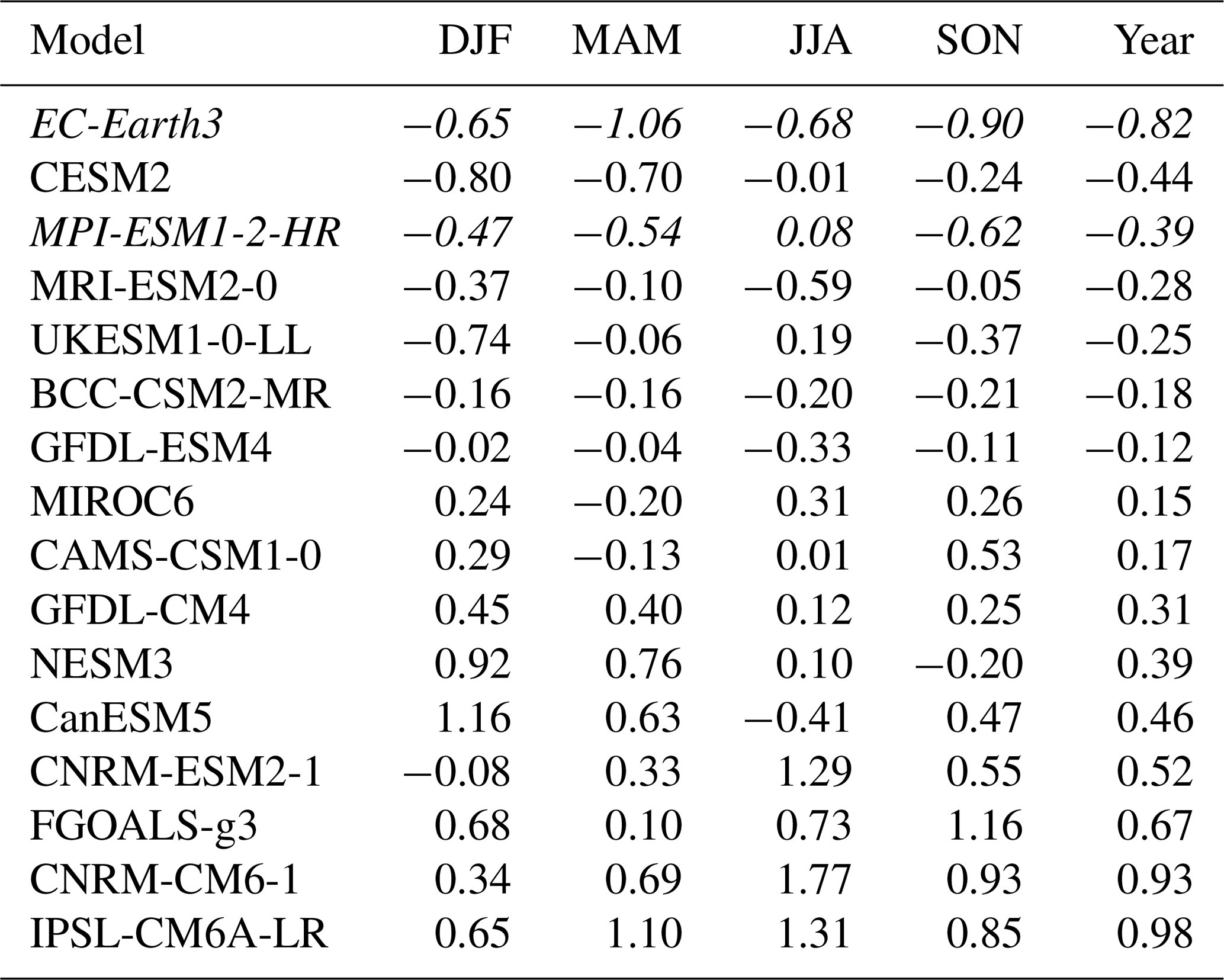
The best-performing models are those with the lowest (i.e. most negative) values of RMSE(χ)_i,norm. This normalisation allowed us to combine them into one score by computing the weighted mean of the three variables:

$$\begin{array}{}\text{(A2)}& S_i={\displaystyle \frac{\begin{array}{c}\mathrm{RMSE}{\left(\mathrm{T}\mathrm{700}\right)}_{i,\mathrm{norm}}+\mathrm{RMSE}{\left(\mathrm{Z}\mathrm{500}\right)}_{i,\mathrm{norm}}\\ +\frac{\mathrm{1}}{\mathrm{2}}\mathrm{RMSE}{\left(\mathrm{SST}\right)}_{i,\mathrm{norm}}\end{array}}{\mathrm{3}}}\end{array}$$

We chose a half weight for the SST because it is less relevant than the other two variables for downscaling in the Alps. The scores are given in Table A1.

Although the CESM2 model shows the second lowest score, we did not select it as it has climate sensitivity close to EC-Earth3. To explore a larger range of climate sensitivities, we thus selected instead the third best, MPI-ESM1-2-HR.

Appendix B: MAR output data and surface energy balance

The outputs of the version 3.10 experiments are available at different height and pressure levels (2, 10, 50, 100 m and 925, 850, 800, 700, 600, 500, 200 hPa for the daily mean temperature), and the first 3 sigma levels (for Tmax and Tmin).

The version 3.14 experiment is available at 2, 10, 100 m and 850, 700, 600, 500, 200 hPa for the daily mean temperature, and the first two sigma levels for Tmax and Tmin. Its output also features the melt/freeze top, GF, HAcc, and SWt variables unlike version 3.10.

Figure B1 describes the surface energy balance in the soil and snow routine in MAR. It is computed for the top layer, which is 1 mm thick when there is no snow on the ground, and of variable thickness when there is snow (depending on the amount of recent snowfall and the evolution of the snowpack).

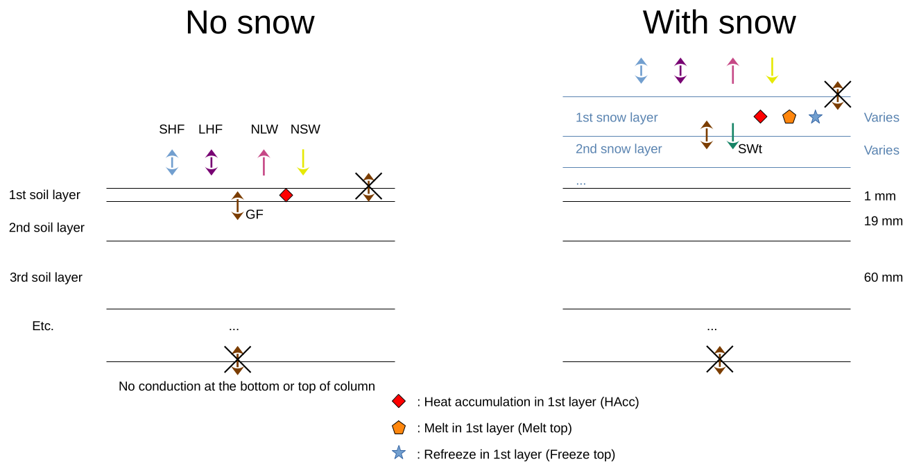
Figure B1 Surface energy balance variables in MAR soil and snow routine, with and without snow on the ground. MAR has a total of 6 soil layers and up to 20 snow layers.

Appendix C: Comparison of MAR simulations to gridded observation datasets

In this section, we briefly compare the MAR simulations at 7km resolution used in our study to gridded observational datasets based on station interpolation and gap-filled satellite observations.

C1 Temperature

We use E-OBS as a reference to validate MAR daily mean temperature at 2 m. E-OBS is a high resolution (0.1°×0.1°) gridded dataset over Europe based on daily station time series from the European Climate Assessment & Dataset (ECA&D). It uses an interpolation algorithm to produce an ensemble of reconstructions (Cornes et al., 2018). We use here the ensemble mean for daily mean air temperature in the version 29 of the dataset.

Figure C1 shows the annual cycle of the three historical simulations of MAR and E-OBS, together with the bias with respect to E-OBS. We can see that all three MAR simulations are in good agreement for the annual cycle of temperature in the Alps in the historical period, although the MAR-MPI v3.14 simulation tends to be a bit colder, especially in spring and early summer (by up to 1 °C) both at low (Fig. C1a and c) and high elevations (Fig. C1b and d). Comparing them to E-OBS for low elevations, they present a warm bias reaching over 2 °C in summer and winter and the MAR-MPI v3.14 presents a cold bias reaching 1 °C in spring (Fig. C1c). For high elevations, the bias is shifted by 1.5 °C towards lower temperatures (Fig. C1d).

Figure C2 shows the maps of the temperature bias over the historical period for the MAR GCM-driven simulations compared to E-OBS.

With some exceptions, all three simulations have similar biases compared to E-OBS. A cold bias at high elevations of about 3 °C stands out for all simulations and all seasons. In summer, the lowlands present a warm bias of around 2 °C for MAR-EC-Earth3 and 3 °C for both MAR-MPI simulations, reaching 4 °C in some locations. Autumn and winter show contrasted biases ranging generally from −2 to +2 °C for the former and −3 to +3 °C for the latter. In spring, all simulations show a cold bias to the south of the Alps but show different signs to the north – these also range generally from −2 to +2 °C.

C2 Precipitation

We use APGD as a reference to validate MAR daily mean precipitation. APGD is a pan-Alpine grid dataset based on rain-gauge data using an interpolation method that integrates climatological precipitation-topography relationships (Isotta et al., 2014).

Figure C3 shows the annual cycle of the three historical simulations of MAR and APGD. It demonstrates a lower amount of precipitation in the Alps in MAR-EC-Earth3 than in the MPI simulations near the end of the year at high elevations, and a slightly lower amount of precipitation in MAR-MPI v3.10 during the summer than in the other two MAR simulations. Otherwise, all three MAR simulations are in good agreement. Comparing them to APGD at low elevations, they present a dry bias of up to 2 mmWe from June to October, and present a similar climatology the rest of the year. At high elevations, the dry bias is from June to September, and there is otherwise a clear wet bias reaching over 2 mmWe during the rest of the year.

Figure C4 shows the maps of the daily mean precipitation bias for the period 1971–2008 of the MAR simulations compared to APGD.

All three simulations have once again similar biases. As seen in Fig. C3, there is a positive bias in the Alps, especially at high elevations in winter, spring and autumn. The bias is highest in winter with values reaching up to 7 mm and over 180 % relative to APGD.

In summer, the bias becomes negative in the Alps with values reaching 5 mm for some locations, or over 60 % relative to APGD.

C3 Snow cover duration

We use the SNOW-CCI dataset (Naegeli et al., 2022) as a reference to validate the number of days with snow on the ground in MAR simulations. SNOW-CCI is a satellite observation product that has been gap-filled, using a linear interpolation of the data for windows of missing data with a maximum duration of 10 d (see Lalande et al., 2023). A second algorithm is used to count the number of snow days for each grid cell. A grid cell is considered to have snow if at least 50 % of the grid is covered with snow. To account for the remaining gaps not filled by the abovementioned interpolation, the number of days with snow is extrapolated at the monthly timescale (Derksen et al., 2025) – for x days covered with snow among y available daily data per month, we define the snow cover duration SCD as:

$$\mathrm{SCD}=x/y\times \left[\text{number of days in the month}\right]$$

The extrapolation is performed only if there are at least 15 d of available data in the month.

Figure C5 shows the bias for the mean number of days with snow on the ground per season for the MAR simulations compared to the SNOW-CCI dataset. The three simulations again show similar biases: there is a positive bias at high elevations in summer and autumn up to 60 d/season, and no bias at low elevations. The positive bias extends to the entire Alps in winter and spring, with winter having additionally a negative bias at low elevations surrounding the Alps of about 20–30 d/season.

This is consistent with the cold temperature and high precipitation bias seen at high elevations (Figs. C2 and C4).

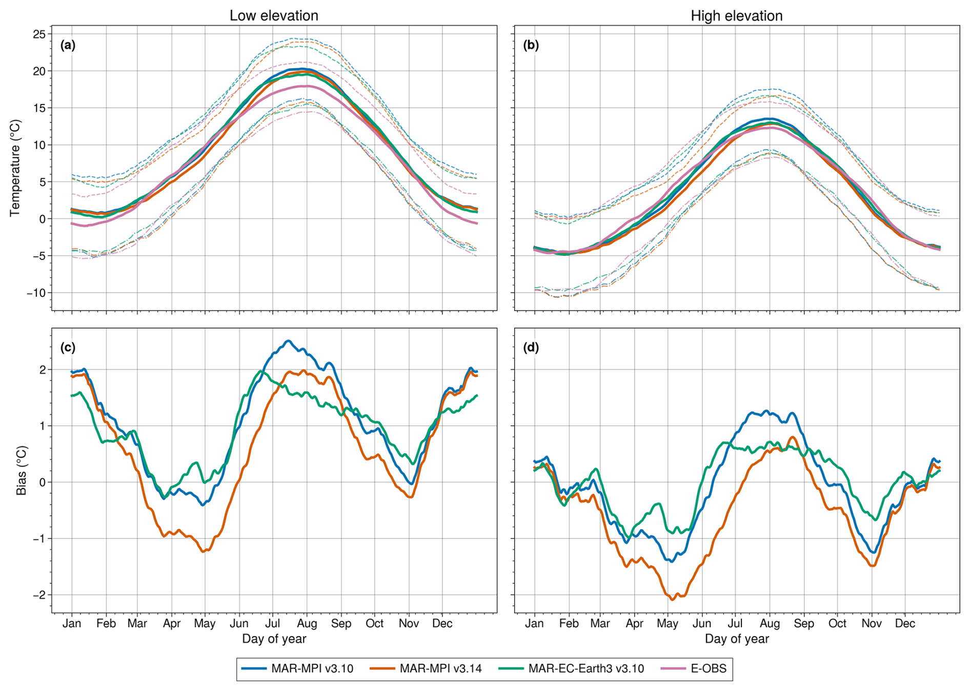
Figure C1 (a, b): Daily mean temperature at 2 m (T2m), averaged over 1961–2014 and over the Alps for low elevations (< 1200 m a.s.l.) and high elevations (> 1200 m a.s.l.), for the three MAR historical simulations and E-OBS (full lines). The dashed lines represent the 90th percentile and the dashed and dotted lines represent the 10th percentile, over 1961–2014. (c, d): Bias of the three MAR historical simulations compared to E-OBS over the same period. A 30 dy rolling mean has been applied to the data, both in the top and bottom panels.

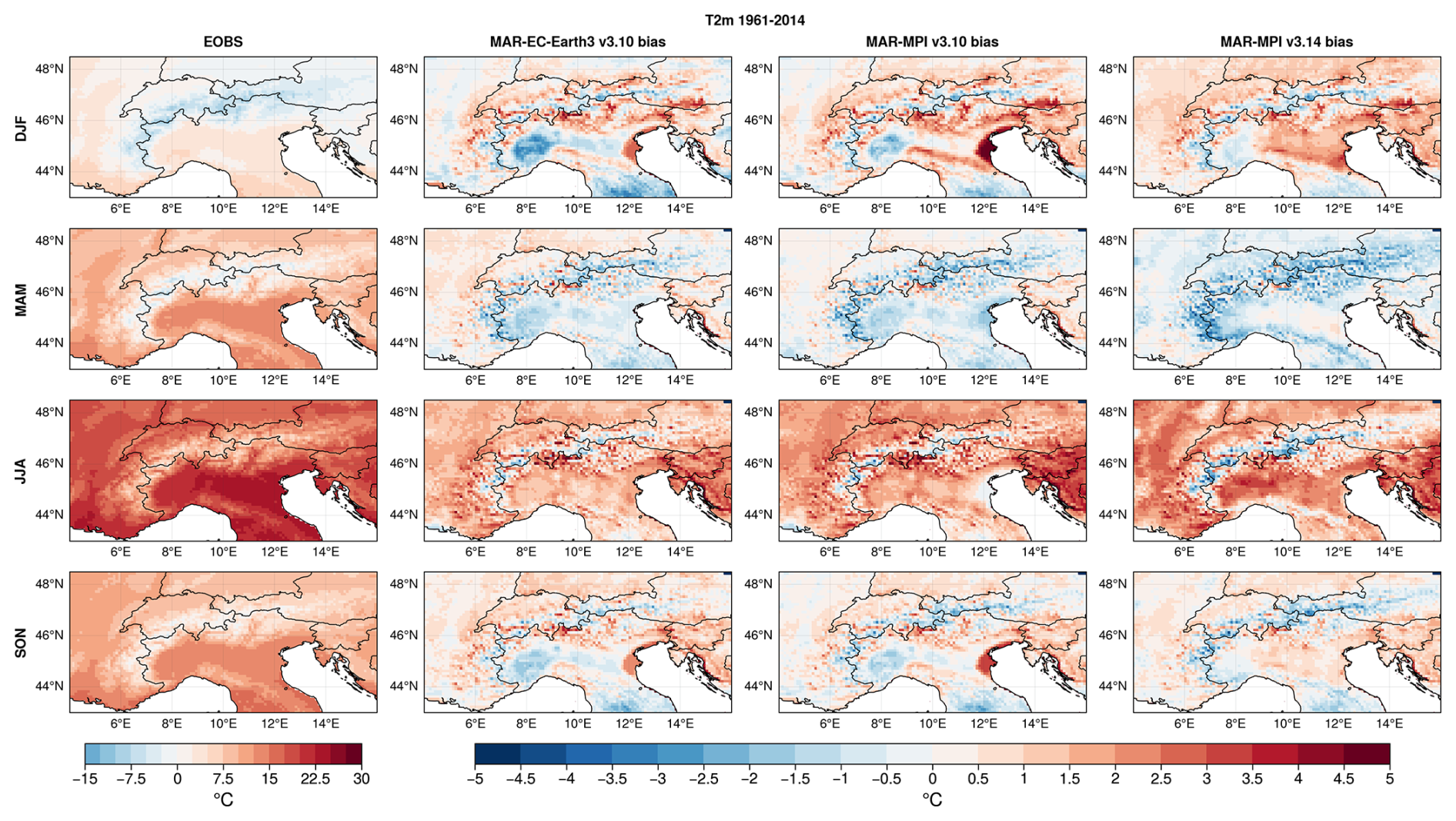
Figure C2 First column: Mean daily temperature at 2 m (T2m) for each season averaged over 1961–2014 for E-OBS. Next three columns: Difference between MAR simulations (forced by EC-Earth3 and MPI-ESM1-2-HR using version 3.10 of MAR, and by MPI-ESM1-2-HR using version 3.14 of MAR for the 2nd, 3rd and 4th columns respectively) and E-OBS over the same period.

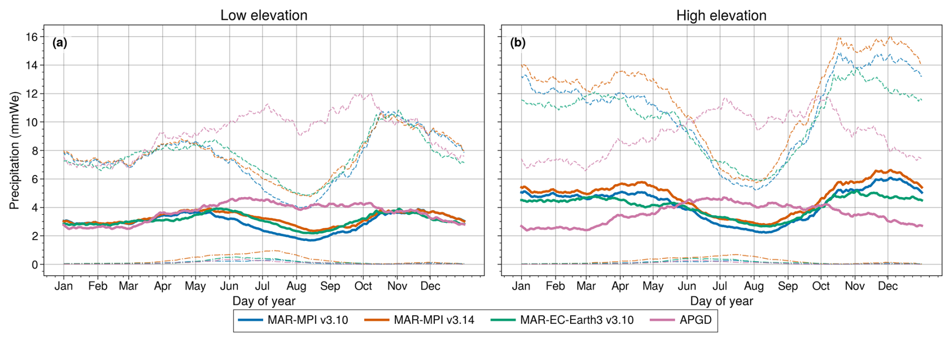
Figure C3 Daily mean precipitation in mmWe, averaged over 1971–2008 and over the Alps for low elevations (< 1200 m a.s.l.) and high elevations (> 1200 m a.s.l.), for the three MAR historical simulations and APGD (full lines). The dashed lines represent the 90th percentile and the dashed and dotted lines represent the 10th percentile, over 1971–2008.

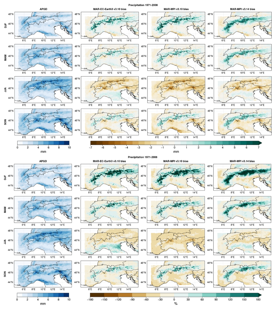
Figure C4 Same as Fig. C2 but for daily mean precipitation, using APGD – top panel is the absolute bias (in mmWe), bottom panel is the relative bias (in percent).

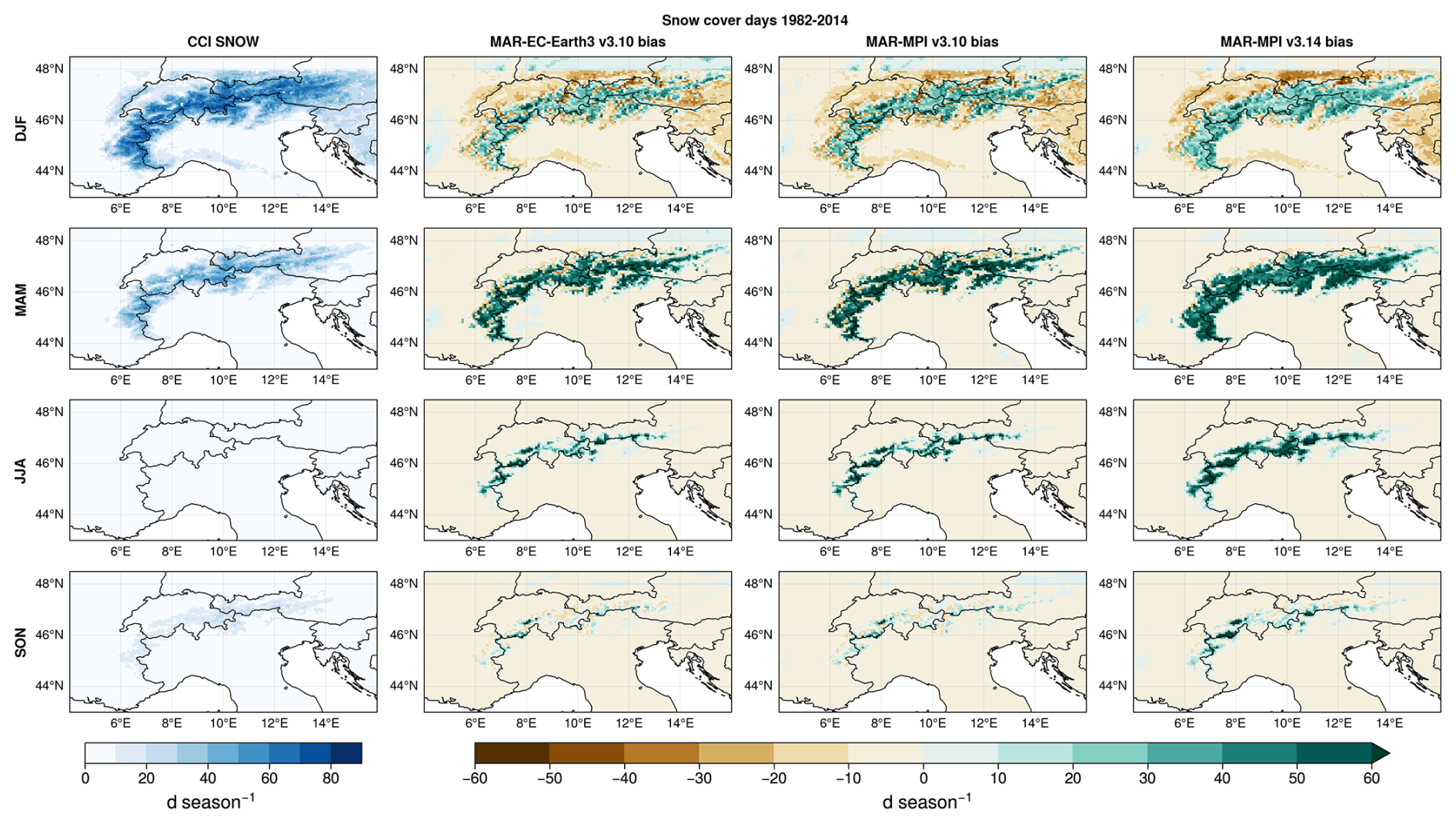
Figure C5 Same as Fig. C2 but for the number of days per season with snow on the ground, using SNOW-CCI. A grid point in MAR is considered to have snow if it has > 50 mmWe of snow.

Appendix D: GCM warming splines

Figure D1 shows the smoothed warming in the GCMs used to force the MAR simulations used in this study. All three start at 14 °C global temperature and rise (from least to most) by 2.4 °C for MPI-ESM1-2-HR using the SSP2-4.5 scenario, 3.6 °C for EC-Earth3 with the same scenario, and 4.5 °C for MPI-ESM1-2-HR using the SSP5-8.5 scenario by the end of the 21st century.

Using these three experiments to force MAR allows us to have a spread in the forcings at the simulations' boundaries.

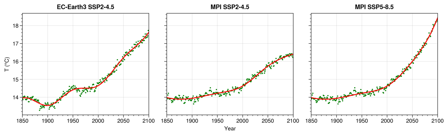
Figure D1 Spline fit (red) of yearly global warming at 2 m average series (green) in the forcing GCM simulations. We used a 3rd degree B-spline with 4 kn.

Appendix E: Elevation of maximum trend

Figure E1 shows the method used to identify the elevation of the maximum warming, by smoothing the data with a spline.

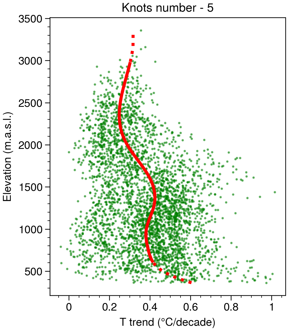
Figure E1 Warming in the Alps during a given 50-year window, with a fit using a 3rd degree B-spline using 5 kn (red). Green dots are the warming for individual grid points. Dashed line: full spline. Full line: we cut off 10 % of the lower elevations and 0.3 % of the highest to ensure that we target the local maximum around 1500 m.