
the Creative Commons Attribution 4.0 License.
the Creative Commons Attribution 4.0 License.
 | 19 Nov 2026
Spatial patterns in indirect effects of human activity on climate, land, and water: comparing top-down and bottom-up clustering approaches

Steven J. Lade
C. Kendra Gotangco Gonzales
Ingo Fetzer
Nitin Chaudhary
Juan C. Rocha
In order to assess the full systemic impact of anthropogenic pressures on climate and land, it is crucial to account for indirect impacts mediated by bio-geophysical processes. These impacts typically display a high spatial heterogeneity. In this study, we systematically compare the ability of top-down and bottom-up clustering approaches to capture the spatial patterns in indirect effects on climate, land, and water. Effect sizes are estimated based on simulations conducted with an offline global spatial vegetation model. Following a top-down approach, we map the resulting global pattern on common natural partitions of the Earth. Cluster validity indices reveal a close alignment between the indirect impacts of land use change on climate and an Earth partition into biomes. In contrast, the indirect impacts of climate- and land use change on surface water runoff are best captured by the Köppen-Geiger climate zones. Adopting a bottom-up approach, we employ multivariate spatially constrained clustering to derive an integrative global partition. Several patches of tropical rainforest on the Indomalayan islands as well as large areas of warm grasslands in Australia are identified as high-impact clusters. The results of this study should be considered illustrative as they are based on only one dynamical vegetation model. Nevertheless, they emphasize the local nature of indirect impacts and elucidate the potential and limitations of both top-down and bottom-up spatial aggregation.
- Article
(28664 KB) - Full-text XML
-
Supplement
(484 KB) - BibTeX
- EndNote


Anthropogenic pressures on critical Earth system processes are continuously increasing and have driven the Earth beyond its safe operating space (Richardson et al., 2023). This underscores the necessity for a more profound understanding and governance of these pressures (Gupta et al., 2024). However, understanding the impact of a human disturbance often goes beyond assessing solely its direct effect – it further requires accounting for the biophysical interplay between different Earth system processes, leading to so-called indirect impacts. For example, while we consider the decrease in natural vegetation as the direct impact of deforestation, the effects of this decrease on carbon storage and water availability are considered indirect impacts. Hence, direct impacts involve human pressure and one Earth system process, while indirect impacts involve human pressure and two Earth system processes. In particular, we refer to impacts as one-way cause-and effect relations, not including feedback mechanisms.
On a global level, taking account of indirect impacts can amplify the measured impact of disturbances in many cases (Lade et al., 2020). At the local level, the situation is much more complex, as a multitude of studies on the interplay between climate change, vegetation cover, and the water cycle demonstrate (Piao et al., 2007; Jong et al., 2013; Sterling et al., 2013; Ito and Inatomi, 2012; Zhou et al., 2023). The magnitude of these effects can vary strongly across regions and corresponding studies typically report them in a spatially aggregated format, based on established Earth partitions (“top-down approach”). For instance, Cramer et al. (2001) and Tobian et al. (2024) assess the effects of climate change for different vegetation zones. Luo et al. (2008) consider these effects depending on the climate zone, while Betts et al. (2007) aggregate them by continent. Koirala et al. (2017) quantify groundwater-vegetation interplay by climate zone in combination with forest type, Lade et al. (2021b) average interaction strengths by continent and dominant functional vegetation type. However, any type of aggregation comes at the cost of information loss, and it remains unclear if these aggregation approaches are indeed fit for purpose. In particular, a classification by functional vegetation type generally does not represent patterns of terrestrial carbon, water, and energy flux regimes; it might even obscure the real world behavior of ecosystems (Page et al., 2023). Instead, other ecosystem characteristics, such as soil attributes, topography, or site hydrology and disturbance, might be essential to capture these functional regimes (Page et al., 2023). So why aggregate at all? Beyond a reduction in computational costs (Priesner et al., 2026), usability and communicability of results play a crucial role. Especially in studies at the interface between science and policy, established clusters rather than a highly resolved pattern can increase accessibility and encourage the use of scientific findings in decision-making.
In this study, we compare widely-used top-down clusterings in their ability to capture the spatial pattern of indirect impacts of human pressures on climate and land. Our analysis covers a wide range of classification criteria, spanning geographical, climatic and biotic dimensions, providing insights into potential drivers of the different effects. Going one step further, we contrast this approach with a classical “bottom-up” approach, based on multivariate clustering with soft spatial constraints (Chavent et al., 2018). While intuitively superior in clustering quality, resulting clusters are harder to interpret and communicate, which may account for its limited use. The integrative Earth partition sheds light on the local interplay of indirect impacts, acknowledging the fact that from a systemic view, such an integration is substantial for a holistic assessment of anthropogenic pressures (Lade et al., 2021b).
We quantify indirect impacts on climate, land, and water in a 0.5° spatial resolution (Sect. 2.1). The resulting global maps form the basis for a top-down clustering (Sect. 2.2) and bottom-up clustering approach (Sect. 2.3). The quality of a clustering is assessed via clustering validity indices (Sect. 2.4). Figure 1 illustrates the structure of this study.
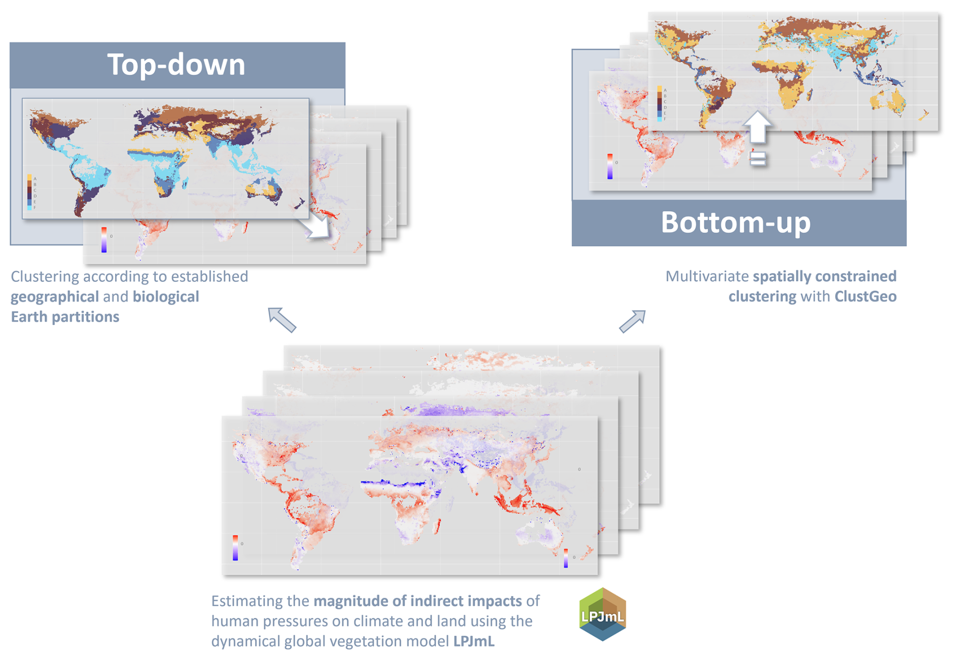
Figure 1Conceptual workflow. In a first step, we estimate the magnitude of indirect impacts of human pressures on climate and land leveraging the dynamical global vegetation model LPJmL. Based on the resulting maps, we compare the ability of established Earth partitions to capture the resulting spatial patterns (top-down approach), and we derive optimal partitions applying the clustering algorithm ClustGeo (top-down approach).
2.1 Estimating the strength of indirect impacts
We estimate the magnitude of the effects of change in atmospheric CO2 concentration on surface water runoff and natural vegetation cover, as well as the magnitude of the effects of land use change on surface water runoff and carbon storage density (Fig. 2). The selected indicators of climate, land, and water align closely with variables representing human pressures, such as emitting CO2, clearing land, extracting water, making the results particularly suitable for an implementation in an impact framework. The estimates rely on LPJmL 4.0.002 simulation outcomes at a 0.5° spatial resolution for the years 1901 to 2013, as being provided by Lade et al. (2021b). Simulations are driven by the re-analysis dataset CRU TS3.21, a monthly climate dataset over all land domains except Antarctica, derived from an extensive network of weather observation stations (Harris et al., 2014). The one-way coupling of the model allows isolating particular effects without the need to disentangle overlapping feedback effects. Runs are repeated with and without human land use, represented by the conversion of natural vegetation to cropland (Schaphoff et al., 2018b). We extract the following variables per year and per 0.5° by 0.5° tile from each run: the percentage of the tile covered by natural vegetation as a proxy of the land component, the surface water runoff density (mm yr−1) as a proxy of the water component, and the carbon storage density (g m−2) as one of the proxies of the climate component. Note that in line with Lade et al. (2021b), we use only vegetation carbon, omitting litter and soil carbon. While largely following the estimation procedure by Lade et al. (2021b), our quantification of land use slightly differs. It rather aligns with the measure of biosphere integrity used by the Earth Commission, which measures the amount of natural ecosystems below which some ecosystem services are lost (Mohamed et al., 2024).
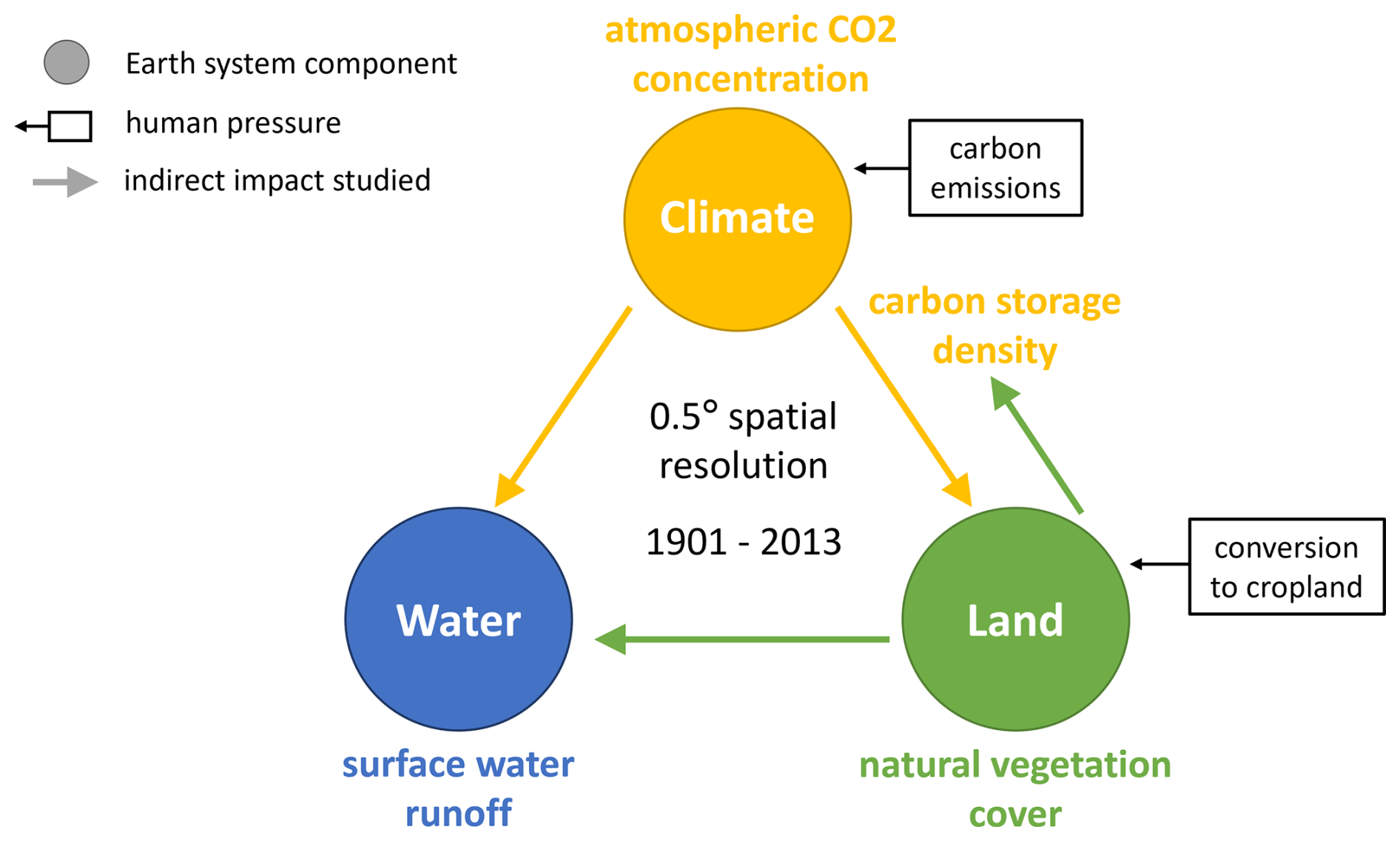
Figure 2Modeling set-up. We use LPJmL simulation outcomes for the years 1901–2013 in a 0.5° spatial resolution to estimate the strength of indirect impacts that human pressures in the form of carbon emissions and in the form of conversion of natural vegetation to cropland have on carbon storage density (climate), natural vegetation cover (land), and surface water runoff (water).
The effects of change in natural vegetation cover are quantified using simple difference quotients. More precisely, its effect on runoff is measured via the difference in average runoff (RO) during the last 30 years of simulations with (wLUC) and without human-driven land use change (noLUC) in a tile, divided by the difference in average vegetation cover (VC) during the last 30 years of simulations with and without human-driven land use change in the same tile, i.e.
The land-use change implementation is based on historical crop functional type allocation merging several sources, including HYDE3, MIRCA2000, and historical irrigation (Dataset 4 in Schaphoff et al., 2018a). The choice of 30 years aligns with the established use of 30-year averages in the investigation of Earth system processes and reduces interannual variability (see e.g., Trewin, 2022). The effect of change in natural vegetation cover on climate, measured via carbon storage density (C), is defined analogously. Observe that, consequently, if the average vegetation cover in a grid cell is the same in the last 30 years of the scenario with and the scenario without land use change, the size of the effect cannot be computed. Acknowledging the fact that the raster approach is more prone to noise than the aggregated approach, we exclude grid cells whose difference in vegetation cover is less than 1 % of the total area, assuming that such marginal changes in human land use can be neglected. The effects of climate change on runoff and vegetation cover are evaluated on the basis of the scenario without human-driven change in land use. In contrast to the first approach, we make use of the total length of the simulation by regressing yearly runoff density/natural vegetation cover per tile on global CO2 concentrations between 1901 and 2013 and, whenever significant (p≤0.05), considering the regression coefficient as magnitude of the respective effect. This magnitude might reflect both direct effects of climate on water, such as through changes in precipitation, and indirect effects mediated through changes in natural vegetation cover, such as variations in the soil infiltration rate. Importantly, LPJmL4 does not include nutrient limitations, which might lead to a general overestimation of the CO2 fertilization effect (Terrer et al., 2019). Note that the two estimation methods do not yield quantitatively comparable results. Accordingly, in this study, we do not compare the absolute size of climate change-induced effects and land use change-induced effects. Furthermore, regarding the potential conversion between the two climate proxies used in this study, note that a decline in carbon storage does not translate linearly into an increase in atmospheric CO2. To diminish the effect of outliers in clustering and cluster validation, we “clip” each of the four data sets to effect-dependent upper and lower boundaries. More precisely, we increase or decrease, respectively, all values below or above certain boundaries [cmin,cmax] to the respective boundary. The boundaries were set to (VC → RO), (VC → C), (C → RO), and (C → VC). For the sensitivity analysis, we repeat the whole estimation procedure relying on LPJmL simulations driven by six different climate models (CanESM2, GFDL-CM3, GFDL-ESM2G, HadGEM2-AO, MIROC-ESM, NorESM1-ME), provided by Lade et al. (2021a).
2.2 The top-down approach: Natural partitions of the Earth
We cluster the spatially resolved indirect impact sizes according to ten base partitions and certain combinations of these partitions (Fig. 3). Continents (N=7) provide an apparent geographical partition (Lade et al., 2021b). The Köppen-Geiger climate classification offers a simple climate partition (Kottek et al., 2006), starting from five main climates, but refined by taking into account precipitation (N=13) and temperature profiles (N=28) (Kottek et al., 2017). Our vegetational Earth partitions are based on the continuous distribution of the dominant plant functional types (PFTs) as defined by the LPJmL global dynamic vegetation model outputs (Schaphoff et al., 2018b). The classification is based on the average fractional cover over the last 30 years of the simulation without human-driven land use. With this choice, we follow both Lade et al. (2021b) and Dinerstein et al. (1995) in their approach to base their classifications on the original land cover before intense human-induced changes. Grid cells are classified as barren land whenever the other eleven plant functional types together cover less than 50 % of the total grid cell area. In the following, we will refer to barren land as a PFT as well (N=12). Aggregating plant functional types into five main types (N=6) following major regional attributes yields a coarser partition, while characterizing tiles by their two (N=24) and three (N=59) most dominant PFTs results in finer partitions. Biogeographic realms (N=6) have been defined as continent- or sub-continent-sized areas with unifying geographical, floral, and faunal features (Udvardy, 1975; Dinerstein et al., 2017). Each realm can be further divided into different biomes (N=15), characterized by a comparable climatic regime, similar vegetation structure and spatial patterns of biodiversity (Dinerstein et al., 1995; Ostberg et al., 2013). Biome classification is based on the averaged results of the last 30 years of the LPJmL simulation without human-driven land use. We furthermore consider combinations, “overlaps”, of two partitions each, by classifying tiles according to their respective classes in both partitions. Simply put, if partition A distinguishes between classes A1 and A2, and partition B between classes B1 and B2, the combined partition AB consists of classes A1B1, A1B2, A2B1, and A2B2. We combine each of the rough partitions (continents, main climate types, realms, and main PFTs) with all other partitions except for their own refinements. Figure 3 illustrates the combination scheme using the example of continents. Note that we do not consider the overlap of continents and realms due to their high similarity. Maps of all base partitions can be found in Appendix A.
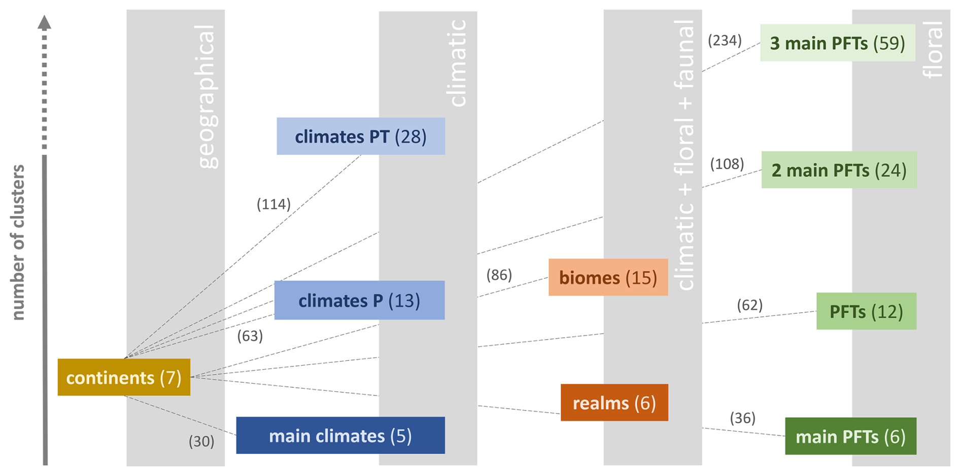
Figure 3Creating combined Earth partitions. Base partitions are ordered along the x-axis according to the nature of their classification criteria and along the y-axis according to their number of clusters. As exemplarily depicted for continents, we furthermore create combined partitions. The numbers in brackets indicate the number of clusters. (Nomenclature: climates P = main climates + precipitation conditions, climates PT = main climates + precipitation conditions + temperature conditions (compare Table B1), PFTs = plant functional types as defined by LPJmL, classification by the (one/two/three) most dominant PFTs in a tile).
2.3 The bottom-up approach: Spatially constrained clustering
In preparation for the multivariate clustering, we reduce the data space to tiles in which the natural vegetation cover does differ between the simulation with human-driven land use change and the one without (35.800 out of 67.420 tiles). This pre-processing step makes sure that all four effect-types can be estimated on each tile considered and thereby reduces a potential bias towards certain effect types in the cluster validity indices. Furthermore, to reduce biases in the clustering results, we rescaled the data set for each effect to by dividing each value by the maximal absolute value of the respective effect size.
The R-package ClustGeo provides a hierarchical clustering algorithm with spatial constraints, taking into account both the similarities in the “feature space” (in our case the four effect variables) and the similarities in the “constraint space”, defined by spatial attributes of the data points (Chavent et al., 2018). For our analyses, we use Euclidean distances between multivariate effect sizes to measure similarity in the feature space.
We implement similarity in the constraint space in two different ways. At first, in form of a simple binary matrix, where a “1” denotes that two grid cells are horizontally, vertically, or diagonally neighboring. This definition of similarity leads, loosely speaking, to topologically “smooth” clusters. Nevertheless, since ClustGeo is based on soft spatial constraints only, clusters can consist of several unconnected, geographically dispersed components. This mimics the shape of the clusters in many of the top-down partitions considered in this study. Therefore, the neighborhood-based similarity measure is well-suited for comparing the performance of top-down and bottom-up partitions.
For an aggregation into geographically more interpretable clusters, we repeat the clustering procedure defining dissimilarity in the constraint space as geographic distance between the tiles' centroids. Intuitively, basing the definition of dissimilarity on distance rather than neighborhood typically results in less smooth, but spatially more compact clusters.
The so-called mixing parameter allows us to balance geographic cohesion and homogeneity within the group in the resulting partition. Increasing α from 0 will result in topologically/spatially more compact clusters, potentially at the cost of similarity of effect size within clusters.
We repeat the clustering procedure for various combinations of the number of clusters K and the mixing parameter α. We range K from 5 to 255 in steps of 10 and α from 0.1 to 0.7 in steps of 0.2.
2.4 Measuring clustering performance
We assess the quality of both natural Earth partitions and bottom-up clusterings via established cluster validity indices. Typically, the quality of a partition is characterized by two aspects: the similarity of the elements within a cluster (“compactness” or “homogeneity”), and the distance between clusters in the feature space (“separation”) (Todeschini et al., 2024).
Assume that n objects are being clustered in K disjoint clusters. Let d be the number of variables (i.e., the dimension of the feature space) and x the d-dimensional feature vector of object x. Here, m denotes the d-dimensional vector of variable means, mk the d-dimensional vector of cluster means. We denote by nk the number of objects of the cluster k. We use the notation for the Euclidean norm of a vector.
Independently of the underlying clustering, the total variability in the dataset is measured by the Total sum of squares
It consists of the Between-cluster sum of squares
quantifying the variability between clusters, and the Within-cluster sum of squares . Typically, a large BSS or, equivalently, a small WSS are indicative of good cluster quality. Here, we consider an alternative to the WSS, the Banfield-Raftery index
which is better adapted to large differences in cluster size (Todeschini et al., 2024). For a slightly different angle of perspective (although, of course, not independent), we further consider the R-squared index
which quantifies the fraction of total variability in the data set that is explained by the differences between clusters. Consequently, a value close to 1 is typically more desirable than a value close to 0.
Compared to the extensive patterns of indirect impacts of land use change (Fig. 4A–B), the indirect impacts of climate change on water runoff and natural vegetation cover exhibit more “patchy” patterns without a clear dominance in sign (Fig. 4C–D). This phenomenon reflects the complex effects of increasing levels of atmospheric carbon concentration on the vegetation (Zhou et al., 2023). Furthermore, in many regions, we observe only weak or no significant indirect impacts of climate change, which may be partly due to opposite effects canceling each other out. Both phenomena are also likely to be exacerbated by differences in the methods used to estimate effect sizes (see Methods). We provide a detailed discussion of the spatially resolved maps and a comparison to corresponding studies in Appendix C. Potential mechanisms underlying positive and negative effect sizes are summarized in Fig. 5.
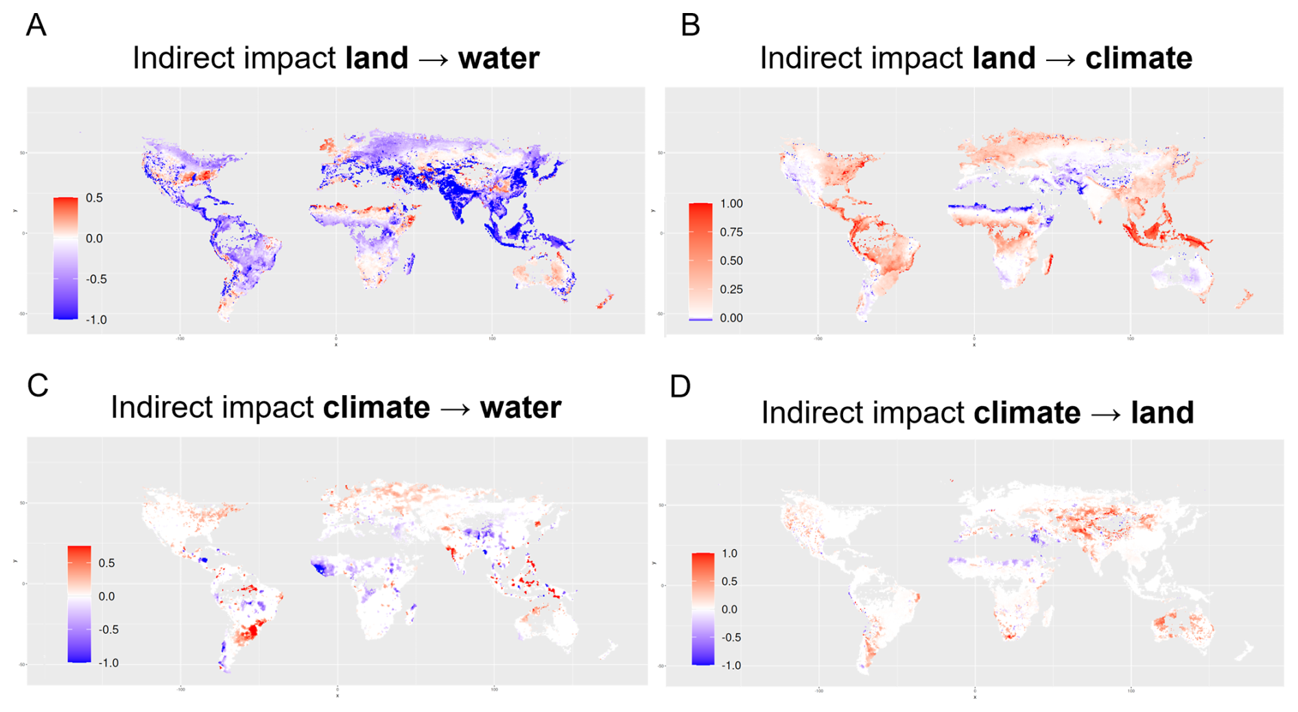
Figure 4Global patterns of indirect impacts. The maps show the scaled effect sizes of changes in natural vegetation cover on (A) surface water runoff and on (B) carbon storage and of changes in atmospheric carbon dioxide concentration on (C) surface water runoff and on (D) natural vegetation cover. A positive effect size (red) indicates that an increase in one Earth system process (e.g., increased atmospheric CO2 concentration) causes an increase in another Earth system process (e.g., increased surface water runoff). Analogously, negative effect size (blue) indicates that an increase in one process leads to a decrease in another. Note that for clarity, the color scale varies across effect types and directions and therefore should not be used for cross-comparisons. All maps are restricted to grid cells in which the cover of natural vegetation has changed by more than 1 % of the cell area between the simulations with and without human-driven land use change (see Methods). World maps showing the larger area of estimated effects of climate change on surface water runoff and natural vegetation cover can be found in Fig. G1.
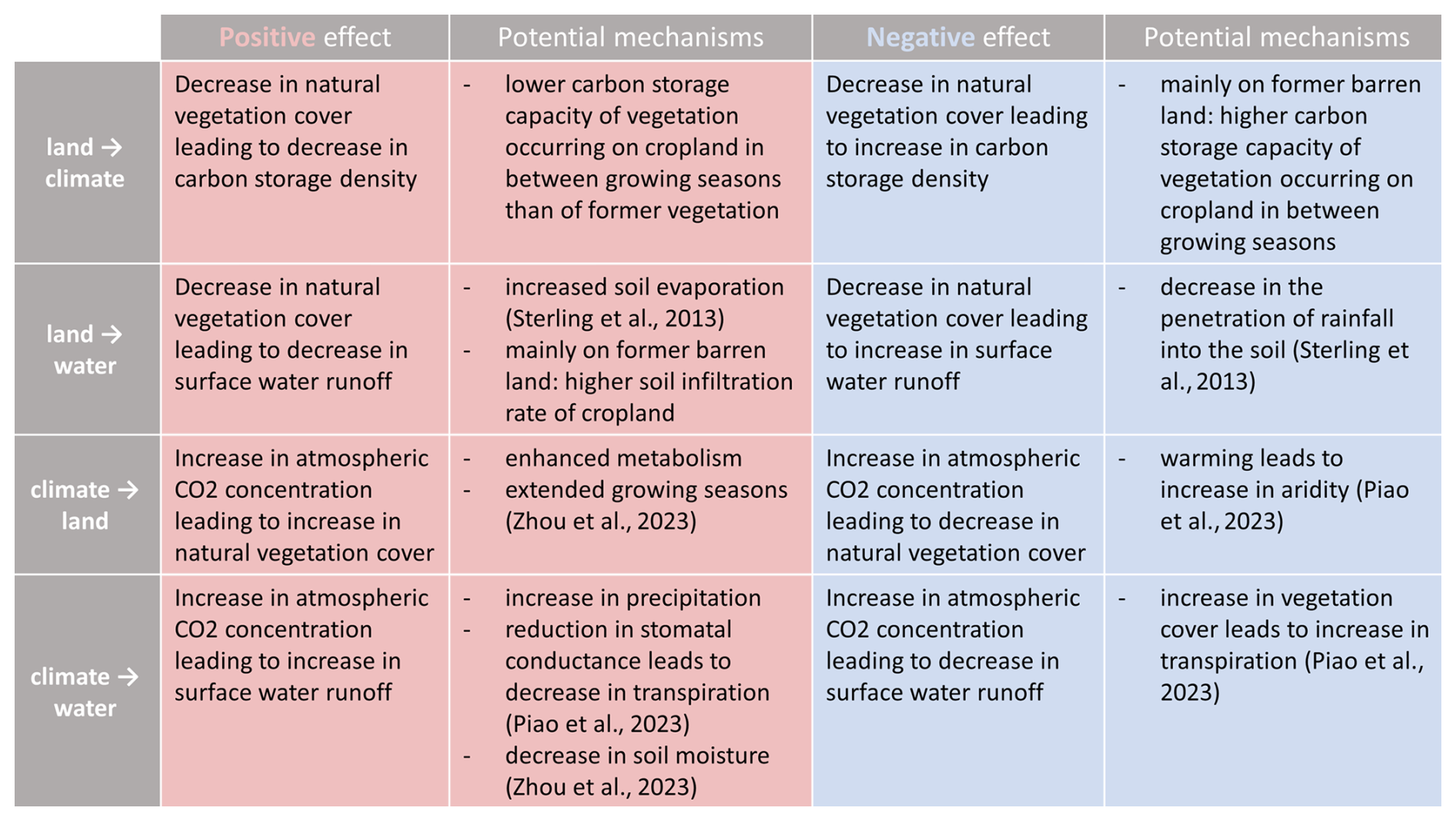
Figure 5Potential mechanisms underlying positive and negative effect sizes of land use change and climate change. Note that a decrease in natural vegetation cover denotes the replacement of natural vegetation (including barren land) by cropland.
3.1 Comparing the clustering quality of top-down and bottom-up partitions
With respect to explained variability, the selected top-down partitions are in general clearly outperformed by the bottom-up partitions. The R-squared index of the neighborhood-based bottom-up partitions without spatial constraints (α=0) converges towards a value of 1 for all four effect types (Fig. 6). With increasing spatial constraints (), within-cluster variability naturally increases, leading to a lower between-cluster variability and thereby to a decrease in the R-squared index. Nevertheless, in most cases there remains a large gap in explained variability between the bottom-up and the top-down partitions, which do not exceed values of 0.3 for the effects of climate change (Fig. 6C and D) and values of 0.5 for the effect of land use change on water runoff (Fig. 6A). Only for the effect of land use change on climate, RS indices exceed values of 0.7, indicating that more than 70 % of the total variance in size of indirect impacts is explained by the variance among cluster means (Fig. 6B). The high performance in this particular case might be traced back to the fact that measuring the effect of land use change on vegetation carbon density provides a very direct and unconfounded approximation. As such, its strength reflects the vegetational and climatic characteristics of an area – each of which are captured by several top-down partitions and, in a combined fashion, by the biome framework.
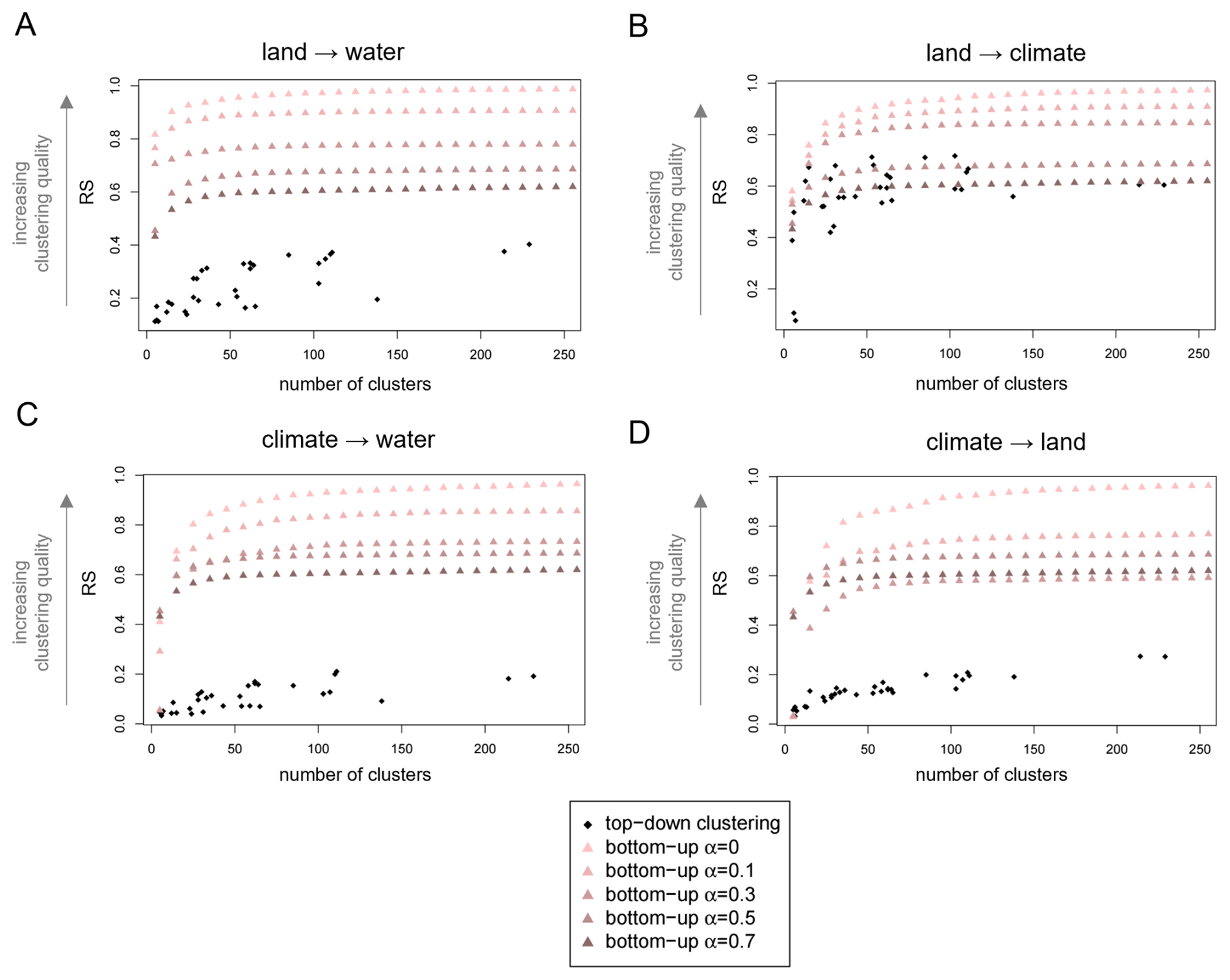
Figure 6Bottom-up clustering substantially outperforms top-down clustering. R-squared index (RS) of the “top-down” geographical, climatic and biological Earth partitions and of the “bottom-up” neighborhood-based partitions without (α=0), and with increasing spatial constraints , and 0.7. Performance is evaluated separately based on the one-dimensional feature space of effect size for (A) the effect of land on water, (B) land on climate, (C) climate on water, and (D) climate on land, respectively. The partitions are sorted by their number of clusters. Intuitively, the RS index increases with increasing number of clusters k and the algorithm yields the best results without spatial constraints (α=0).
If performance is being assessed via within-cluster variability (BR index), the difference between the two approaches is not as clear. Intuitively, the BR index overall increases with increasing spatial constraints (Fig. F1). Interestingly, for the effects of climate change (Fig. F1C and D), top-down partitions show a smaller within-cluster variability than equally-sized bottom-up partitions under strong spatial constraints (α=0.5 and α=0.7). For the effect of land use change on climate, some of the top-down partitions perform even better than the corresponding unconstrained bottom-up partitions (Fig. F1B). There are several reasons why the unconstrained clustering algorithm might not always produce a clustering that optimizes the BR index. Firstly, the algorithm minimizes with respect to a slightly different measure of within-cluster variance. Secondly, the algorithm optimizes at each step, meaning it can end up in local rather than global optima (compare e.g., Chavent et al., 2018).
3.2 The top-down approach
3.2.1 Identifying drivers of indirect impacts
We consider a partition to represent a spatial pattern “best” when its RS/BR index is higher/lower than that of partitions with a similar number of clusters. The corresponding classification criteria suggest potential environmental drivers of the observed pattern. We find that the effects of land use- and climate change on surface water runoff are generally best represented by climate-based partitions (Fig. 7A and C). The BR indices align with this trend (see Fig. D1A and C). With an RS value of 0.37, the classification by continent and Köppen-Geiger climate zone (climates PT) is among the best matches for the pattern of the land → water effect, suggesting that the impacts of land use change on surface water runoff are meaningfully influenced by precipitation- and temperature conditions.
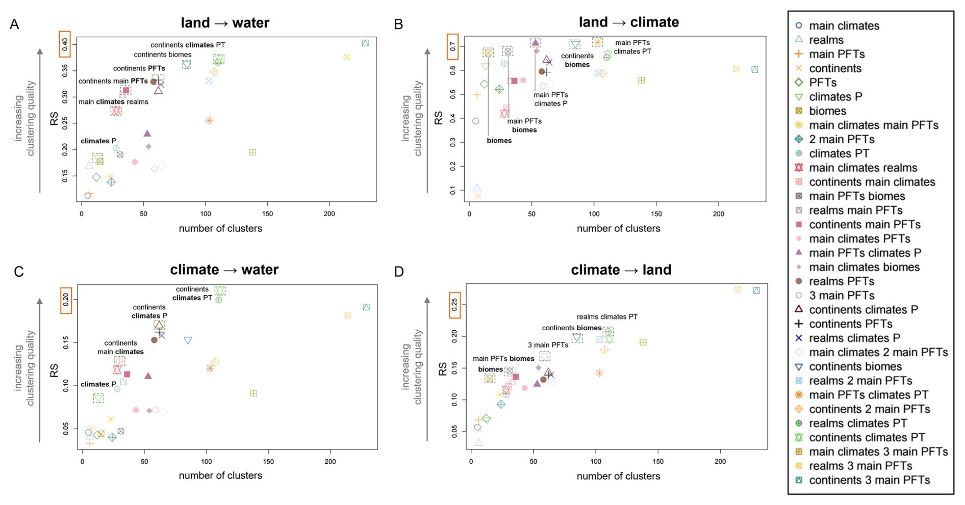
Figure 7Spatial patterns of individual indirect impacts are best explained by different natural classification criteria. R-squared index (RS) of the 33 geographical, climatic, and biological Earth partitions with respect to the magnitude of the effects of land use change on (A) surface water runoff and (B) carbon storage, as well as the magnitude of the effects of change in carbon dioxide concentration on (C) surface water runoff and (D) natural vegetation cover. The partitions are sorted by their number of clusters k and highlighted by a square if they stand out in performance compared to partitions of similar number of clusters.
With an significantly lower RS index of 0.21, the same partition still provides the best match for the global pattern of the climate → water effect. The overall similar means and high standard deviations across the clusters (Fig. H2B) align with the generally weak performance of the cluster validity indices and demonstrate the apparent mismatch between the “patchy” pattern of effect size and the more extensive Köppen-Geiger climate zones.
The top-down partitions yield the overall highest RS values and the smallest BR values for the effect of land use change on climate (Figs. 7B, D1B). Here, it is the biome-based partitions that stand out in performance. The classification by continent and biome yields an RS value of 0.71, indicating that the differences between the means of the underlying 85 clusters explain more than 70 % of the total variability in the dataset. The high clustering performance is evident in the close correspondence between biome boundaries and the separation of regions with different effect sizes (Fig. H3) and visually supported through the well-separated means of effect size across the clusters (Fig. H3B)
For the effect of climate change on natural vegetation cover, we observe a similar trend towards biome-based partitions as for the reverse effect of land use change on climate (Figs. 7D, D1D). Since those partitions combine climatic and vegetational characteristics, we consider this outcome to be a proof of concept rather than a new insight. However, in contrast to the high correspondence between the top-down partitions and the land → climate effect, RS indices do not exceed values of 0.3 in the case of the climate → land effect. Consequently, just like for the effect of climate change on water, cluster means are generally not well separated across clusters (Fig. H4B). As mentioned earlier, the interplay of different, partly opposing effects of atmospheric changes on the vegetation is likely to result in a complexity which the rather simple top-down partitions considered in this study might not be able to capture. A combination of more than two classification factors and/or the inclusion of further criteria (e.g., topographic factors) might yield further insights.
3.2.2 Revealing the risk of information loss
Multivariate cluster validity indices accounting for all four effect types confirm the previously observed gap in clustering quality.: while RS values exceed 0.9 for bottom-up partitions without spatial constraints and values of 0.5 for α=0.7, they do not exceed values of 0.4 for top-down partitions (Fig. F2A). A similar, albeit smaller discrepancy in performance can be seen for within-cluster variability (Fig. F2B). For partitions of fewer than 100 clusters, the multivariate pattern is best represented by a classification by continent and biome in terms of both explained variability and within-cluster homogeneity (Fig. E1). Larger partitions yield only marginally higher RS indices and lower BR indices. The best-performing partition of fewer than 50 clusters is provided by the classification by continent and main plant functional types, as used in Lade et al. (2021b). However, this aggregation entails a significant loss of information. For the comparison, it should be noted that Lade et al. normalize their interaction strengths with respect to the pre-industrial values of the variables and the estimated guardrails for safe levels of impact. Consequently, they consider increases and decreases in pressure on the respective Earth system processes, which leads to the opposite sign for their interaction value compared to our climate change effect size. For example, consider the effect of land use change on surface water runoff in the temperate forest region in North America. Lade et al. observe a slight negative interaction strength in this cluster (Fig. 3 in Lade et al., 2021b). When averaged across the corresponding tiles, our results corroborate this trend (Fig. I1). However, the spatially resolved effect size in Fig. 4A reveals that the cluster contains a distinctive area of strongly negative effect size along the Mississippi river, which is surrounded by large areas of positive effect size. These opposing effects cancel each other out and, with the positive effect of land use change on runoff being generally slightly lower than the strength of the negative effect, lead to a negative average value. Note that this particular pattern is neither well represented by the climate-based division discussed earlier (Fig. H1). Similarly, in the tropical forests of South America, distinctive areas of positive and areas of negative effects of climate change on runoff (Fig. 4C) cancel each other out, resulting in a negligibly small average effect size for the cluster. As a further example, consider the effect of climate change on water in the tropical forest of Africa (Fig. 4C). We find a negative average effect size in the cluster, which aligns with the results of Lade et al.. However, our approach reveals a hotspot of negative effect size in the Guinean forests, gradually decreasing northwards and eastwards along the forest-savanna ecotone. This remarkable pattern is obscured by the aggregation approach by Lade et al.
3.3 The bottom-up approach
The RS index of the bottom-up partitions converges to values above 0.9 for all four values of α, indicating that more than 90 % of the total variability in the data set is explained by the variability among cluster means (Fig. 8A). The increase in the RS index for an increasing number of clusters is particularly strong for smaller partitions, while the curve clearly flattens with partition size approaching 100. In contrast to the RS index, the Banfield-Raftery BR index displays a weaker convergence and α-dependent differences in quality remain comparatively large even for higher numbers of clusters (Fig. 8B). Considering the univariate R-squared index RS, we find that the bottom-up partitions explain the variability in the effect of land use change on surface water runoff better than the variability in the other effects (Fig. J1). Interestingly, with respect to within-cluster similarity, as being measured by the BR index, the partitions perform best for the effect of climate change on natural vegetation cover (Fig. J2).
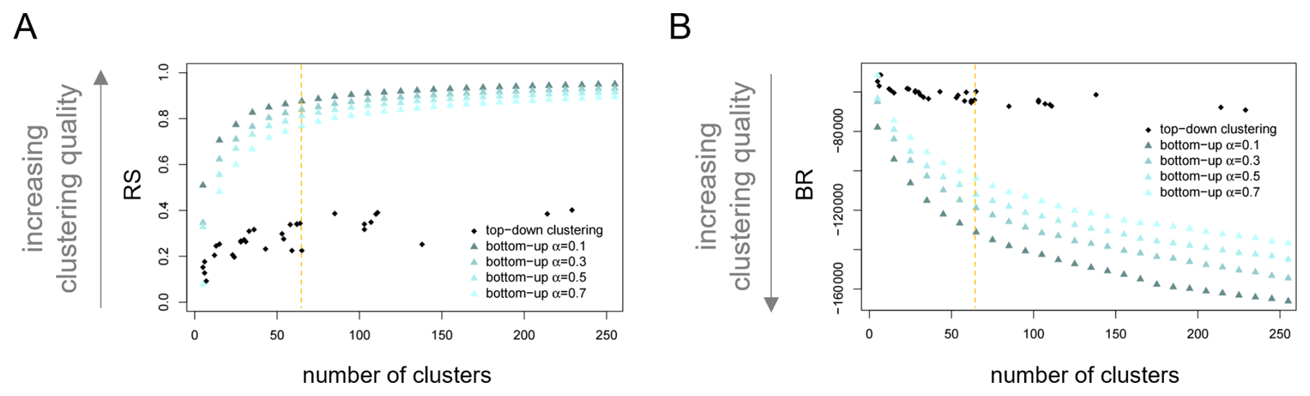
Figure 8Performance of distance-based bottom-up partitions for varying mixing parameter α. (A) R-squared index (RS) and (B) Banfield-Raftery index (BR) for the distance-based bottom-up partitions generated by ClustGeo based on the multidimensional feature space of all four impact types. Indices are displayed for partitions generated with mixing parameter . With increasing α, clustering quality naturally decreases. Partitions are ordered by their number of clusters. The dashed orange lines mark indices for the partition into 65 clusters, which we consider in more detail. For further orientation, we included the metrics of the top-down partitions presented in 3.2.
When aiming for an interpretable, communicable, and high-quality partition of the Earth into impact zones, one needs to find a compromise between a manageable number of clusters (as regulated by K), spatial locality of the clusters (as regulated by α), and both high values of between-cluster variance and within-cluster similarity. While an optimal choice will always be context-specific, we will explore the characteristics and the interpretative potential of impact zones by means of a representative partition of the Earth into 65 impact zones.
With growing α, spatial coherency of the clusters increases (Fig. K1). For α=0.1, some clusters with a certain degree of cohesion and spatial compactness can already be observed, such as in the boreal forests in northern Asia and in the tropical forests of Africa (Fig. K1A). Those impact zones reflect larger areas of uniform effect size in all four effect types, mirroring a natural spatial cohesion (compare Fig. 4). Overall, compared to the top-down partitions, the bottom-up partitions clearly reflect the more “patchy” pattern of effect size for the effects of climate change on water and natural vegetation (Fig. 4C–D). For α=0.7, the partition into 65 impact zones already explains 77 % of the total variability in the multivariate dataset (Fig. 8A) and the high degree of spatial compactness allows observed impact profiles to be interpreted in the context of each cluster’s regional environmental characteristics. In order to highlight patterns in the interplay of effects, our analysis will focus on clusters which stand out in absolute strength for at least two effect types (Fig. 9).
A frequent pattern in the clusters' impact profiles is the interplay of a negative effect of land use change on water and a positive effect of land use change on climate (Fig. K2). These effects should be particularly pronounced in areas of dense vegetation with a high infiltration rate and carbon storage capacity, and indeed, the pattern is especially evident in the tropical forests of South America (Clusters 36 and 52), Africa (Cluster 48), and Asia (Clusters 35, 54, and 44). Cluster 44, which encompasses several patches on the Indomalayan islands, stands out by an additional strong effect of climate change on surface water runoff. A closer inspection on Ecoregions level reveals that those patches largely overlap with montane rain forests and peat swamp forests. This observation suggests that the increase of the atmospheric CO2 concentration leads to a comparably strong increase in surface water runoff in these types of tropical and subtropical moist broadleaf forests. Piao et al. (2007) found a remarkable increase in precipitation across large areas of the Indomalayan islands. Hence, we hypothesize that the remarkable effect on runoff could be resulting from a high sensitivity to increased rainfall due to the typically steep terrain and low infiltration rate of the soil in montane areas and due a potential saturation in peat swamp forests. We mark Cluster 44 as one of the “high impact” clusters, since indirect effect size is particularly strong for three different effects.
A less frequent pattern in the impact profile can be observed in warm savanna and open shrubland regions of Africa (Clusters 39 and 43), as well as in warm grassland regions of Australia (Cluster 60). Here, a human-driven decrease in natural vegetation cover leads to a decrease in surface water runoff and an increase in carbon storage density due to the apparently higher infiltration rate of cropland and the higher storage capacity of vegetation occurring in between growing seasons compared to sparse C4 grass. Cluster 60 is further characterized by a highly positive effect of climate change on natural vegetation cover. We trace this observation back to the climate change-induced increase in precipitation in the area of the later (Piao et al., 2007) and classify the corresponding cluster as high-impact cluster.
In several regions across North America (Cluster 21), Europe (Cluster 3), Asia (Cluster 18), and New Zealand (Cluster 65), we observe positive effects of human-driven land use change on both water runoff and carbon storage. Interestingly, the corresponding clusters all lie within areas that are dominantly covered by temperate forest, mixed with some C3 grass (compare Appendix A). A closer investigation of this relation could be subject of future studies.
Clusters 37, 47, and 38, all dominated by tropical forest mixed with temperate forests or C3 grass, are characterized by highly negative effect sizes of climate change/land use change on surface water runoff. The later indicates that the CO2-induced increases in vegetation cover exceed the effect of CO2-induced decreases in transpiration (Zhou et al., 2023, Fig. 5). Cluster 38, encompassing Honduras and some densely vegetated patches on the Indomalayan Islands, additionally displays a highly positive effect size of land use change on carbon dioxide storage. We therefore classify this cluster as high-impact cluster.
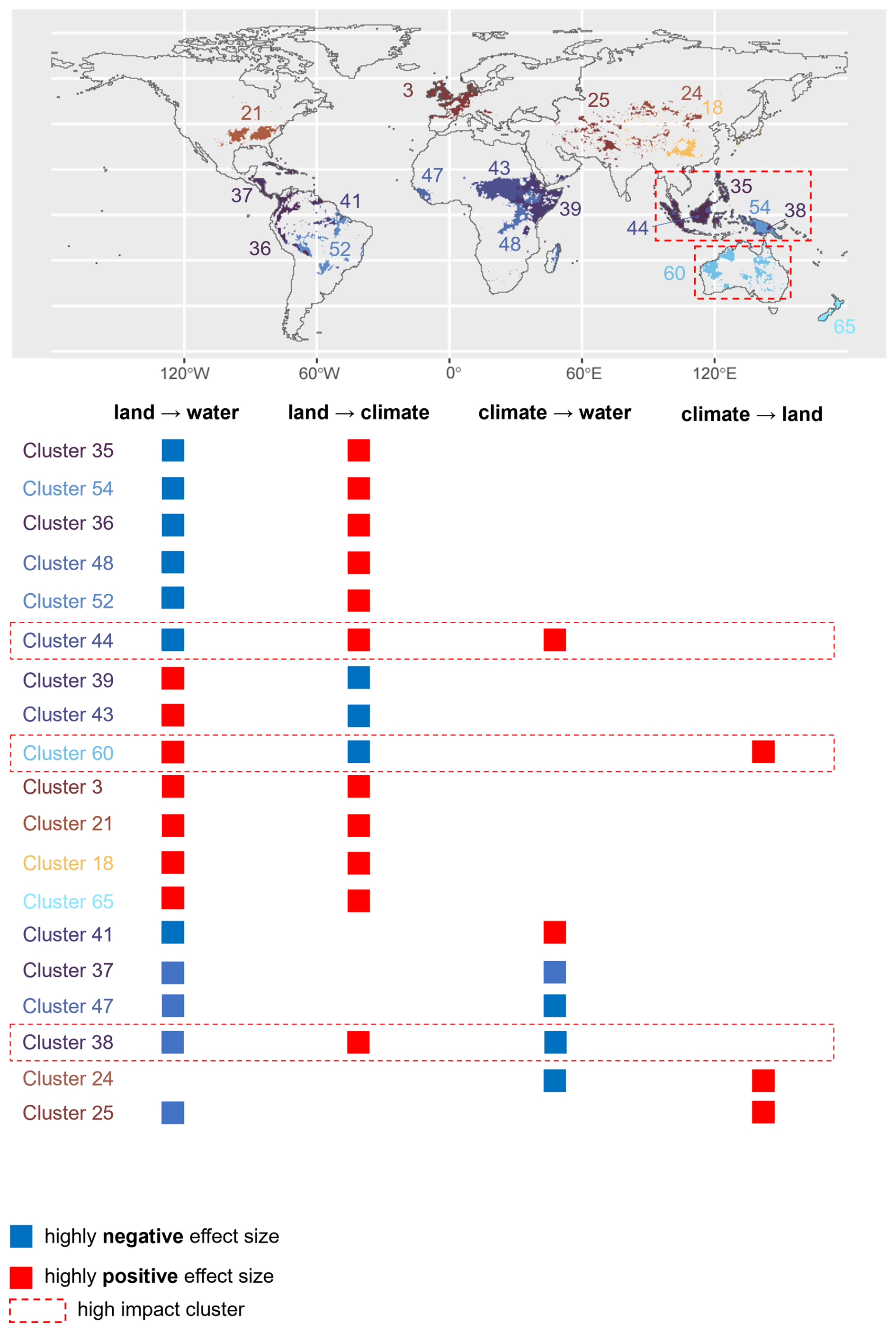
Figure 9Integrative world map of bottom-up impact zones. ClustGeo was applied to derive a partition of 65 clusters based on the four-dimensional feature space of indirect impacts. The constraint space was given by geographical distances, and the mixing parameter α was set to 0.7. The map displays only clusters which stand out in effect size for at least two different effect types. The table lists their corresponding impact profiles. Red tiles indicate highly positive effect size, blue tiles highly negative effect size. Clusters with markedly strong (absolute) size of at least three effects are further emphasized as “high impact” clusters. Color and number code of the clusters aligns with that of the mean and standard deviations in Fig. K2.
3.4 Sensitivity analysis
The global pattern of indirect impacts is stable across climate models for the effects of land use change on surface water runoff and on carbon storage density (Figs. L1 and L2, respectively). Consequently, clustering analyses across all climate models support the observed dominance of climate-based aggregations for the effect on surface water runoff and the observed dominance of biome-based partitions for the effect on carbon storage density (Figs. M1 and M2, respectively). Note, however, that in the latter case, the dominant plant function type consistently appears as a crucial classification criterion as well (Fig. M2). The variation across climate models is more noticeable for the effect of climate change on surface water runoff (Fig. L3). This might be due to the fact that the effect of climate change on runoff is composed of both direct and indirect effects mediated through changes in natural vegetation cover, further amplifying uncertainty. Nevertheless, four out of six climate models support our finding of a highly negative effect size in the tropical forest of Africa, with a hotspot in the Guinean forest. Based on the other two climate models, there is no significantly measurable effect in the corresponding cluster. Two out of four climate models support the highly positive effect size in the fully humid hot summer region in South America, based on the other four models there is no significant effect. While climate-based partitions are still strongly represented among the best-performing aggregations, the dominance across climate models is not as clear as for the historical re-analysis dataset (Fig. M3). With respect to the effect of climate change on natural vegetation cover (Fig. L4), several of the observed patterns, such as the highly positive effect size in the temperate grassland of Asia and South America, are stable across climate models. However, there are two clusters which differ in sign of effect size. While the grasslands of central and eastern Africa are assigned a positive effect size based on three climate models, two of them imply a significant negative effect size. Only two of the climate models support the observed slight tendency towards biome-based partitions in the top-down clustering analysis (Fig. M4C and E), while the others either imply a high similarity of the spatial pattern to vegetation-based partitions or do not show a clear tendency.
3.5 Limitations of the study
The results presented in this manuscript build on simulations driven by historical re-analysis data. This approach naturally entails certain limitations. First of all, the reliability of re-analysis data like the one used in this study shows a strong spatial and temporal variation, reflecting the density of meteorological stations. Station coverage underlying CRU TS3.21 is generally high in large parts of North America (Fig. N1A–D) as well as in central and western Europe (Fig. N1C and D). Other areas, such as large parts of Brazil (Fig. N1A and C) and northern Africa (Fig. N1A and B), are particularly data-sparse in some variables, and respective values are heavily depending on interpolation (Harris et al., 2014). Consequently, results affecting these areas should be interpreted with more caution. However, while this uncertainty might directly translate to the effect size of a single tile, we would like to point out that the main results presented in this manuscript are based on large-scale trends and therefore less sensitive to small deviations in the input data. Our results are based on the choice of specific variables representing the Earth system components of climate, land, and water. While our choice is driven by a potential application of our results in the context of human pressures, the use of other variables could lead to slightly deviating results. For example, while changes in surface water runoff capture both changes in soil moisture and in evapotranspiration, their respective contribution varies across regions (Zhou et al., 2023). Using gross primary production instead of natural vegetation cover as representative of the land component could result in an even closer spatial alignment between effect sizes and dominant plant functional types (Guo et al., 2023). Investigating the relationship between indirect effect sizes and representative variables offers an opportunity for further research. Models are always a simplified representation of reality. In this study, by choosing LPJmL as vegetation model, we opted for a one-way coupling. This implies, in particular, that our model does not directly capture feedback mechanisms, such as changes in natural vegetation cover affecting climate, which in turn, impacts vegetation growth. Furthermore, this study only includes a subset of land-atmosphere mechanisms. For example, we exclude quantification of the biophysical pathways by which changes in natural vegetation cover affect climate, such as through albedo and surface energy fluxes. The albedo effect may run counter to the carbon effect and thereby moderate the net land-climate effect (Chen et al., 2024; Hasler et al., 2024). The inclusion of such processes could be subject of future studies. Furthermore, the estimation methods being used to quantify effect size (difference quotient and linear regression), capture only linear relationships (compare Lade et al., 2021b). More complex causality detection methods (see e.g., Runge et al., 2019) could yield a more refined picture and further enhance the current modeling set-up.
We systematically compared the ability of different spatial aggregation formats to capture the spatial pattern in indirect impacts of human pressures on climate and land. We first adopted a top-down approach, which is widely used due to its ease of interpretation and communication. We found that the spatial pattern of indirect impacts on surface water runoff is best explained by climatic classifications. In contrast, the spatial pattern of indirect impacts of land use change on carbon storage density is best explained by biotic classifications. At the same time, our results clearly demonstrate the caveats that this approach entails, independently of the chosen natural classification. Clustering quality appeared to be substantially higher when following a bottom-up approach. Based on the spatially constrained clustering algorithm ClustGeo, we derived an integrative partition based on the multivariate global pattern of indirect impacts on climate, land, and water. Among the resulting clusters, we identified several patches of tropical rainforest on the Indomalayan islands as well as large areas of warm grassland in Australia as high-impact clusters. However, at the same time, our results illustrate the limitations of the bottom-up approach - there is no “one-size-fits-all” clustering. Ultimately, an appropriate approach will always depend on the context and the target audience. In order to generally move beyond simulation dependencies, a natural - although not trivial - next step would be the extension of our framework to observational time series data. Going beyond the controlled set-up of simulations entails additional challenges such as the identification and the disentanglement of scale- and time-dependency, lagged effects, shared environmental drivers, and general higher-order effects. Eventually, a comparison of simulation- and observation-based world maps of indirect effects of human activity would also provide insights into the usability of LPJmL in future systemic assessments of anthropogenic impact on the Earth.
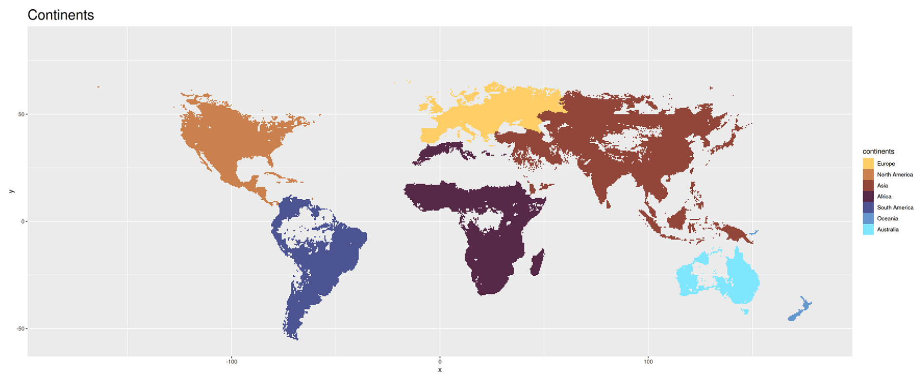
Figure A1Geographic partition of the Earth into continents. Note that all maps in Appendix A display only tiles for which the size of all four effects could be computed (compare Methods).
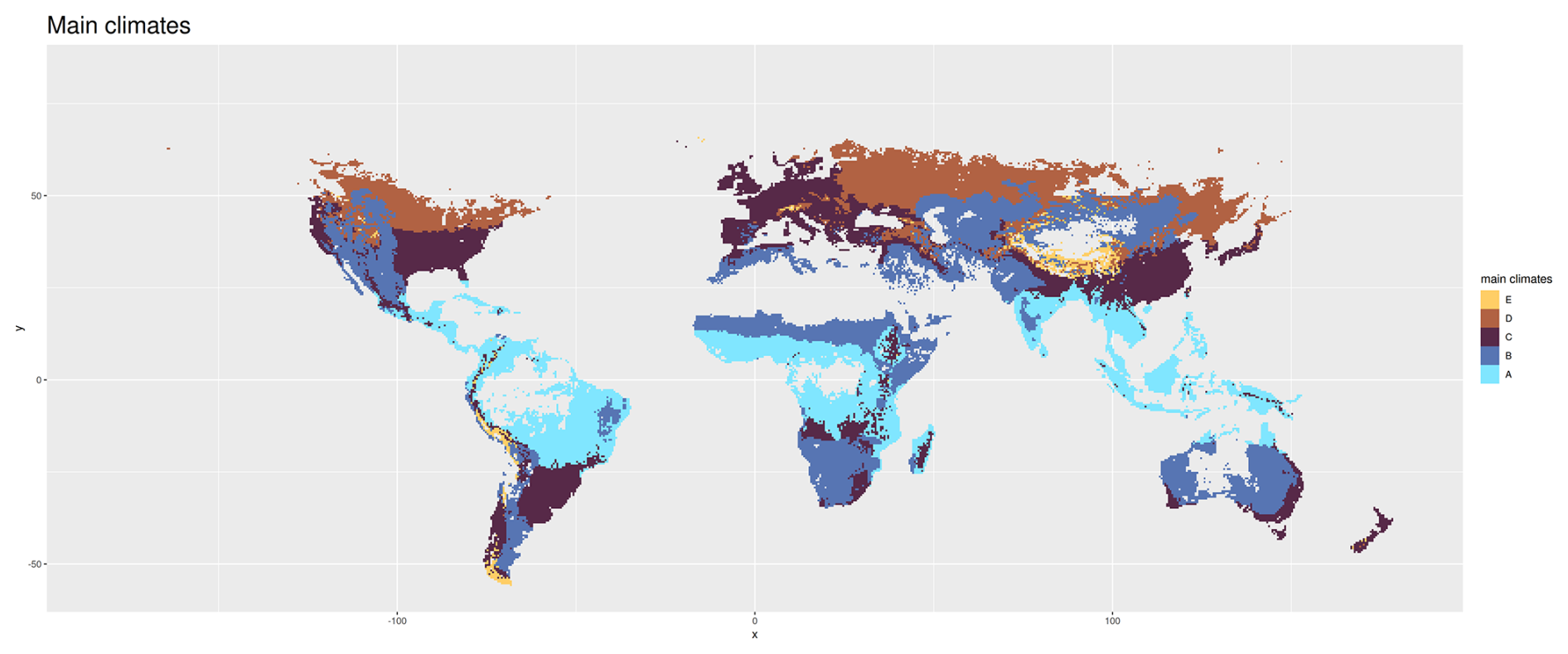
Figure A2Main climates according to the Köppen Geiger climate classification (Kottek et al., 2017). A = equatorial, B = arid, C = Warm Temperate, D = Snow, E = Polar.
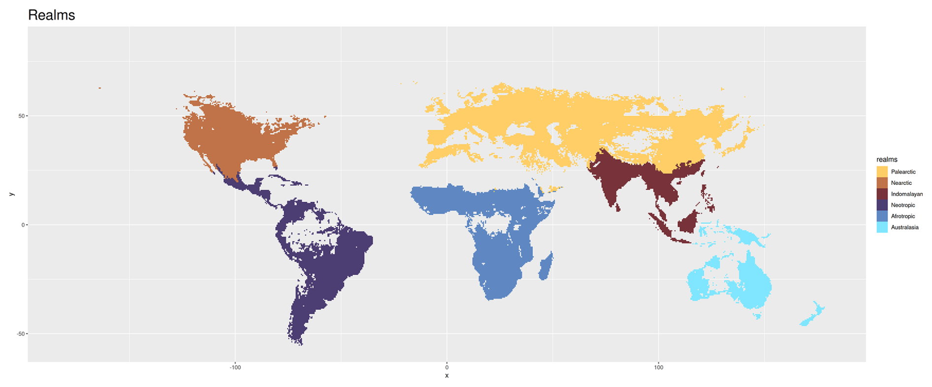
Figure A3Biogeographic partition of the Earth into realms as defined in the Ecoregions framework (Dinerstein et al., 2017).
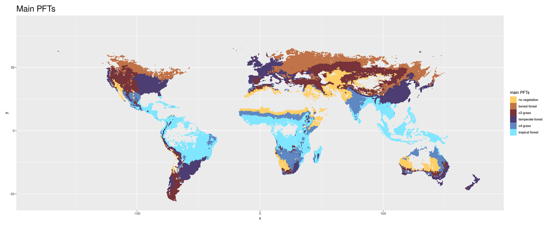
Figure A4Classification based on main dominant plant functional types in LPJmL simulations without human-driven land use (see Methods). Tiles are classified as as “noVeg” if they are predominantly not covered by any vegetation.
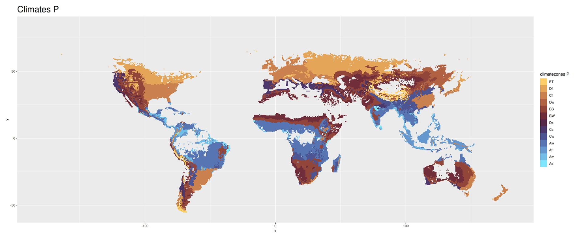
Figure A5Main climate and precipitation types according to the Köppen Geiger climate classification scheme. See Appendix B for the nomenclature.
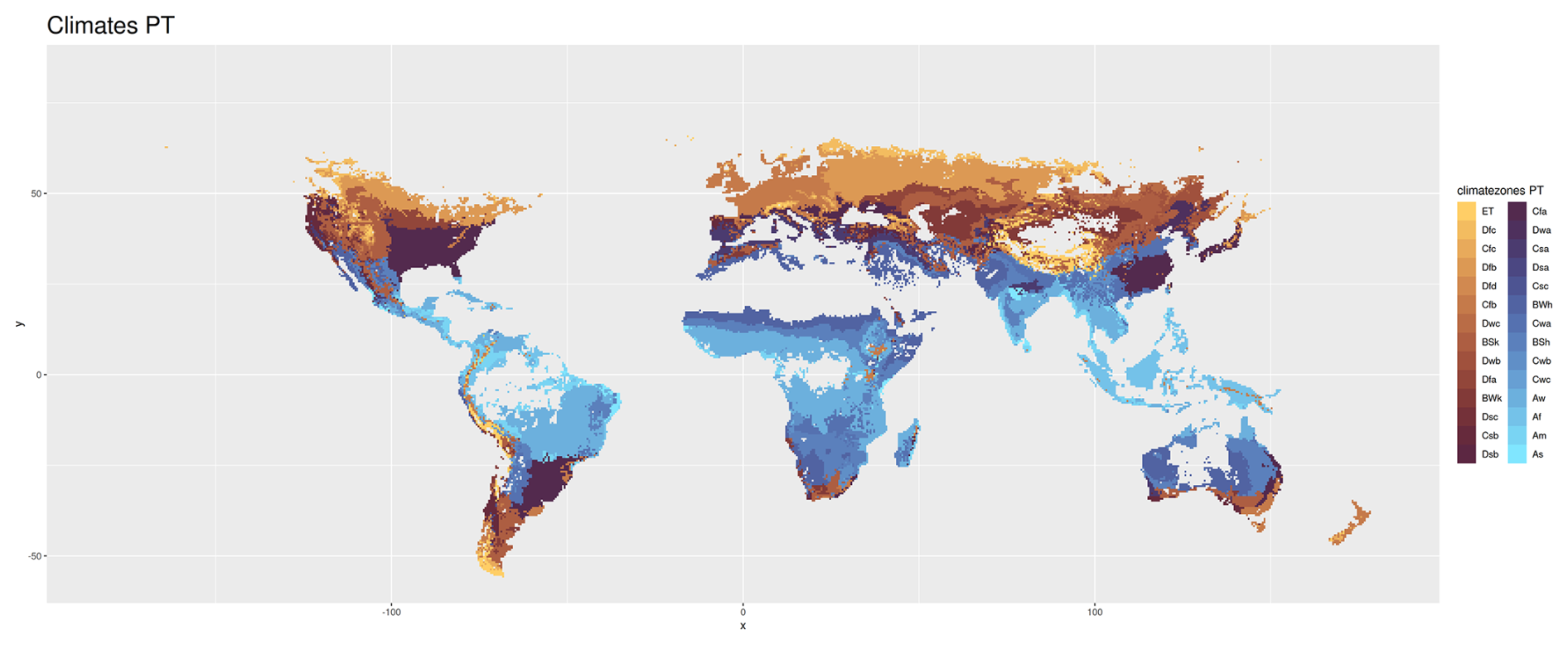
Figure A6Climate zones according to the Köppen Geiger climate classification scheme. See Appendix B for the nomenclature.
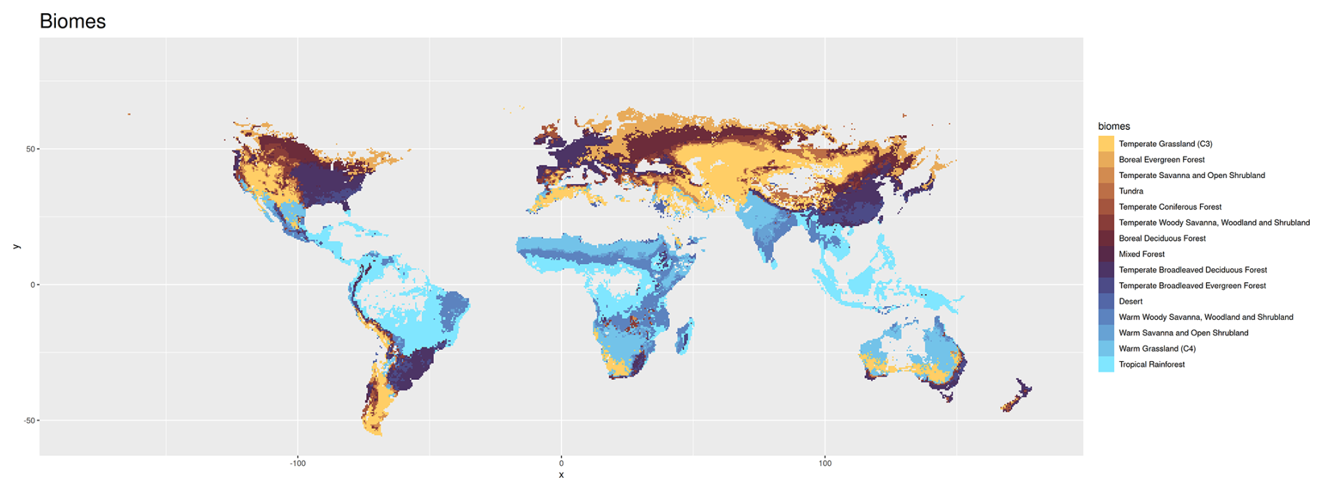
Figure A7Biogeographic partition of the Earth into biomes according to the Ecoregions framework and identified via the Ostberg classification scheme (Ostberg et al., 2013), more recently used in Dinerstein et al. (2017). This scheme is based on parameters produced by LPJmL – the foliar projective cover (FPC) of plant functional types (PFT) and vegetation carbon – to distinguish forests, savannas and shrublands, grasslands and deserts. Types of forests are further classified based on the dominant tree PFTs, while savannas and shrublands consider biomass limits as well as the fractions of trees vs. grasses. Grassland biomes include warm (C4-dominated) vs. temperate grasslands (C3-dominated). The tundra biome is determined using the temperature limits from the climate forcing dataset, the Climate Research Unit (CRU) gridded Time Series (TS) (Harris et al., 2014). The classification is based on the LPJmL simulation without human-driven land use (compare Methods).
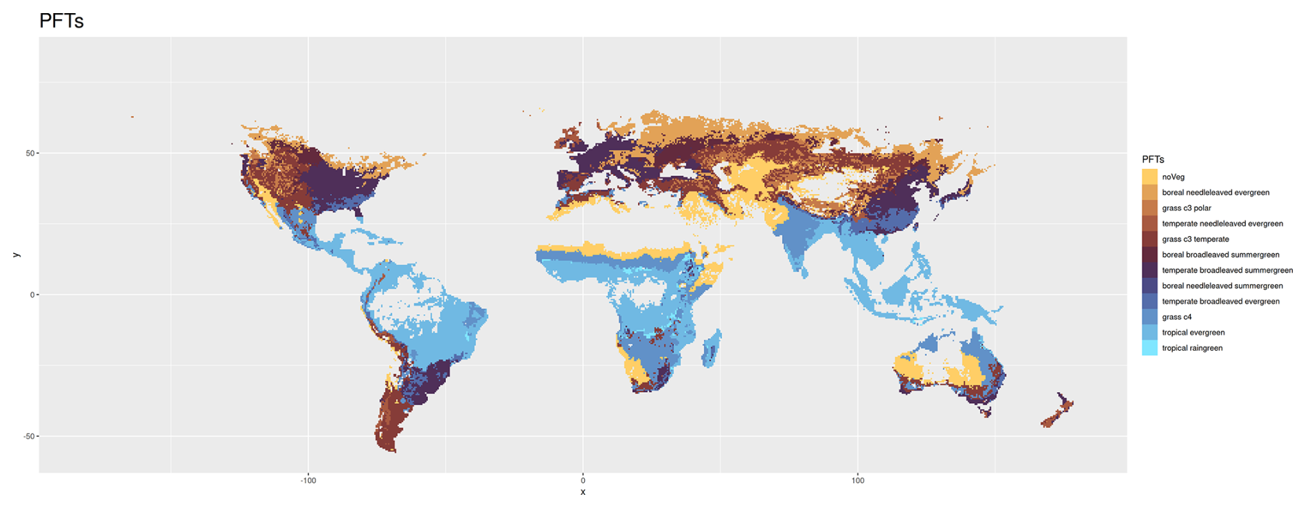
Figure A8Classification into dominant plant functional types based on LPJmL simulations without human-driven land use (see Methods). Tiles are classified as as “no vegetation” if they are predominantly not covered by any vegetation.
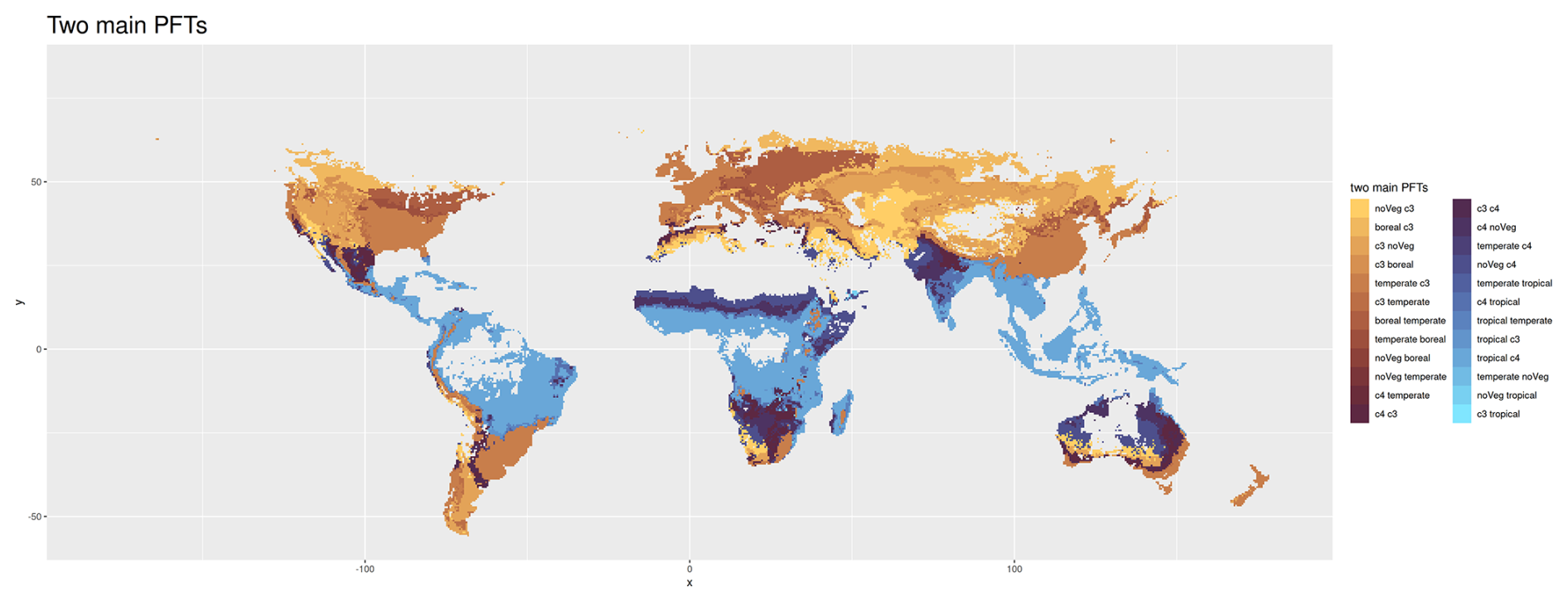
Figure A9Classification based on the two dominant main plant functional types in LPJmL simulations without human-driven land use (see Methods). For the sake of readability, we omit “forest” after boreal, temperate, and tropical, and we omit “grass” after c3 and c4. We use “noVeg” as abbreviation for “no vegetation”. Tiles are classified as as “noVeg” if they are predominantly not covered by any vegetation.
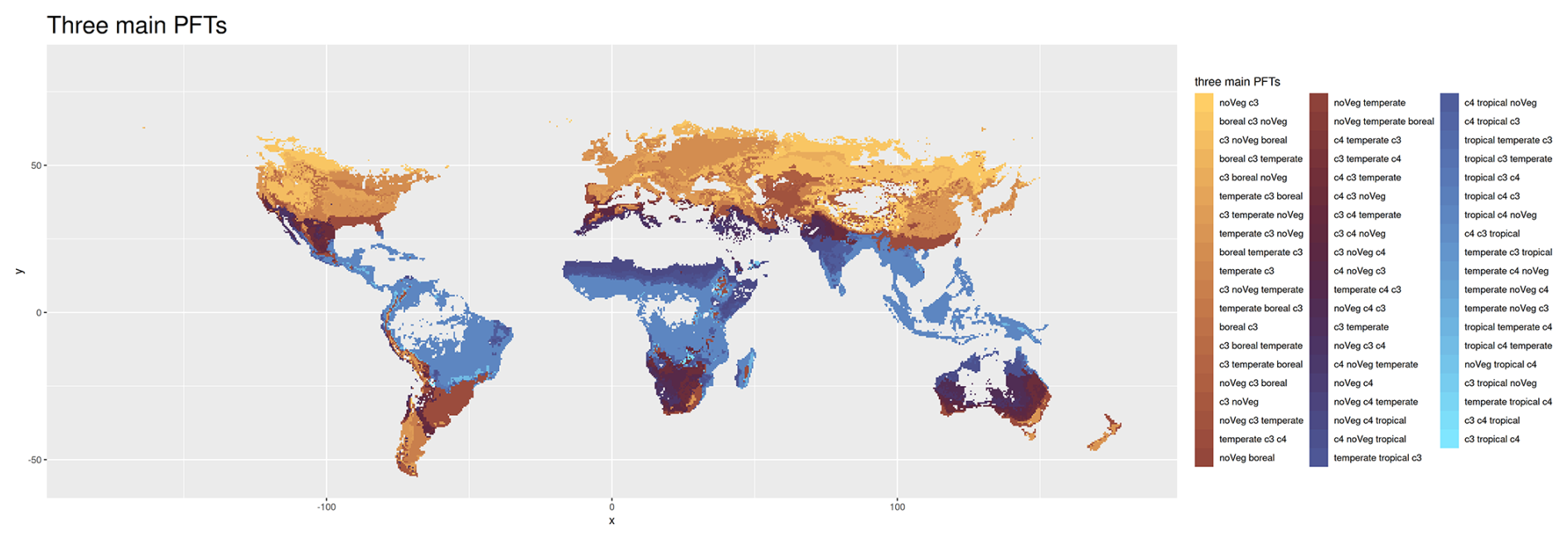
Figure A10Classification based on the three dominant main plant functional types in LPJmL simulations without human-driven land use (see Methods). For the sake of readability, we omit “forest” after boreal, temperate, and tropical, and “grass” after c3 and c4. We use “noVeg” as abbreviation for “no vegetation”. Tiles are classified as “noVeg” if they are predominantly not covered by any vegetation.
Table B1Köppen Geiger climate symbols.
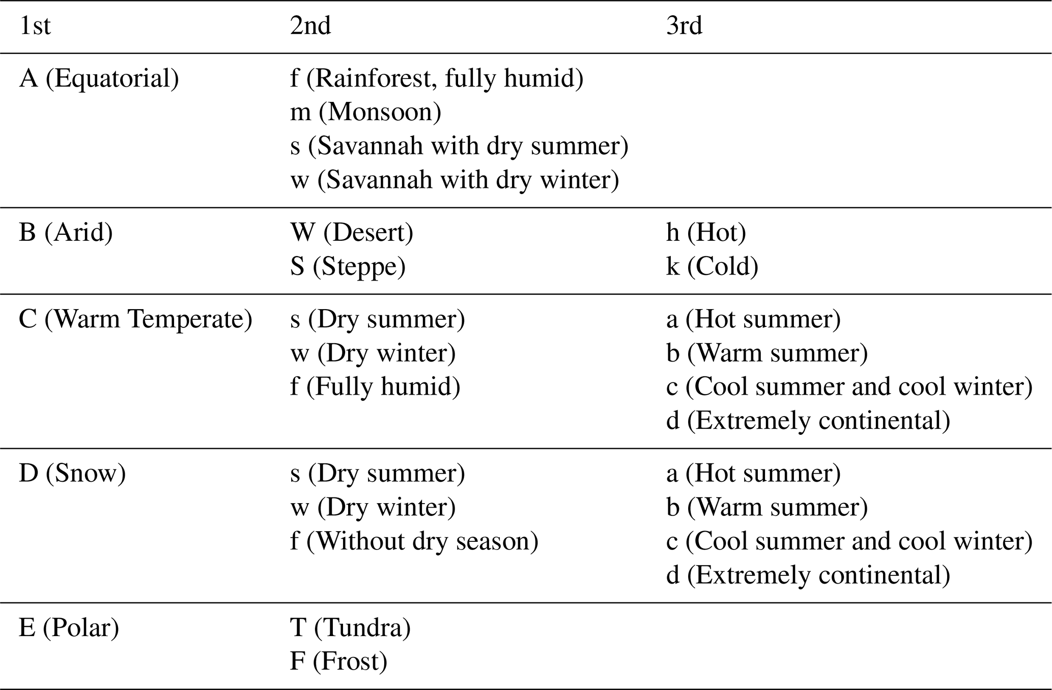
Explanation of the three-letter Köppen Geiger climate symbols. The first letter indicates the main climate, the second letter the precipitation conditions, and the third letter the temperature conditions. Adopted from Kottek et al. (2006).
Our results reveal that a loss of natural vegetation cover driven by the change in human-induced land use causes an increase in surface water runoff in large parts of the world (Fig. 4A). This clear dominance of negative effect size (72 % of grid cells) can be traced back to the fact that deforestation typically leads to a decrease in the penetration of rainfall into the soil and thus to an increase in surface water runoff (Sterling et al., 2013). This effect is especially strong in Asian c4 grasslands and in the Asian tropical forest, which, in undisturbed state, is characterized by a particularly high infiltration rate.
However, in some regions, we observe a slightly to moderately positive effect size, indicating that a decrease in natural vegetation cover leads to a decrease in surface water runoff. In central Australia, southern Africa, and the periphery of the Sahara desert, the most likely reason for this phenomenon is the increased evapotranspiration in these areas (Sterling et al., 2013). Depending on the location, this increase might result from increased soil evaporation due to more exposed soil, or from the higher transpiration of vegetation occurring in between growing seasons compared to formerly largely barren land.
Another factor might be a higher rainfall infiltration rate of cropland in comparison to the former barren soil. Moreover, we find positive effect size in temperate forest regions of Asia, Europe, North America, and South America.
While the transition from areas of negative to areas of positive effect size is typically gradual, it can be remarkably sharp, indicating hard transitions between ecosystems. In some cases, this is due to differences in altitude, such as for the Sichuan Basin in eastern Asia. In other cases, it reflects the distinctive features of river landscapes, such as in the lowland forests along the Mississippi river in eastern North America.
In contrast to the indirect impacts of land use change on runoff, we observe predominantly positive effect size in Fig. 4B (77 % of the grid cells), illustrating that in large parts of the world, a decrease in natural vegetation cover leads to a decrease in carbon dioxide uptake and storage. This effect is particularly high in the tropical forests of South America and Asia, due to their high vegetation content with its high carbon storage capacity (compare Lade et al., 2021b). The formerly barren lands in central Australia, Asia, southern Africa, the peripheral Sahara desert, as well as in North America again display the opposite effect. This is likely due to the fact that the carbon storage capacity of vegetation occurring on cropland in between growing seasons is higher than that of the formerly sparse vegetation.
The spatially resolved effects of climate change on water runoff and natural vegetation cover form more “patchy” patterns without a clear dominance in sign (Fig. 4C–D). This aligns with the high variability of effect size reported in Lade et al. (2021b), reflecting the complex responses to increasing levels of atmospheric carbon concentration (Zhou et al., 2023). The effects of rising CO2-levels include both radiative and physiological forcing. Radiative forcing directly influences precipitation, air temperature, and radiation. Changes in these climate variables can affect soil moisture and vegetation cover, crucial factors in the partitioning of precipitation into evapotranspiration and runoff. Physiological forcing describes the vegetation's physical responses to increasing levels of atmospheric CO2, such as a reduction in stomatal conductance, which generally decreases transpiration, and an increase in vegetation cover, which typically increases transpiration (Piao et al., 2007). Hence, a deeper understanding of the observed patterns of indirect impacts requires a regional assessment of this balance.
We find several hotspot of positive effect size between climate change and surface water runoff in the tropical forests of Asia, Australia, and South America. This aligns with Zhou et al.'s hypothesis that in the regions where vegetation cover is already close to saturation, increasing levels of atmospheric CO2 mainly lead to a decrease in transpiration and thereby to an increase in runoff (Zhou et al., 2023).
In accordance with Zhou et al., we find climate change-induced increases in vegetation cover in the western United States and on the Tibetan plateau in central Asia (marked by a positive effect size in Fig. 4D). This effect can be traced back to enhanced metabolism and extended growing seasons through warming. With respect to runoff, the increasing vegetation cover possibly sets off the effect of the observed increasing precipitation. Indeed, we find a strong decrease in runoff on the Tibetan plateau (marked by a negative effect size in Fig. 4C), and no significant effect of climate change on runoff in the western United States.
In the boreal forests of Europe, we observe large areas of positive effect size between climate change and runoff. This aligns with Zhou et al.'s hypothesis that the decrease in soil moisture exceeds the effect of increasing vegetation cover in many boreal regions (Zhou et al., 2023).
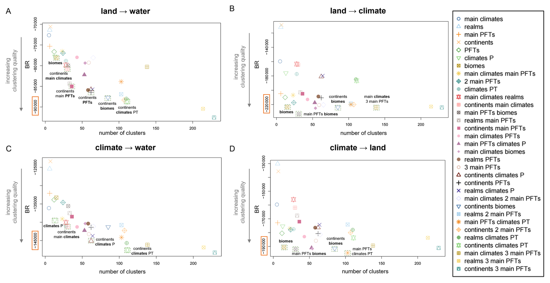
Figure D1Within-cluster similarity of top-down partitions. Banfield-Raftery index (BR) of the 33 geographical, and biological Earth partitions with respect to the magnitude of the effects of natural vegetation cover on (A) surface water runoff and (B) carbon storage, as well as the magnitude of the effects of change in carbon dioxide concentration on (C) surface water runoff and (D) natural vegetation cover. The partitions are sorted by their number of clusters and highlighted if they stand out in performance compared to partitions of similar number of clusters.
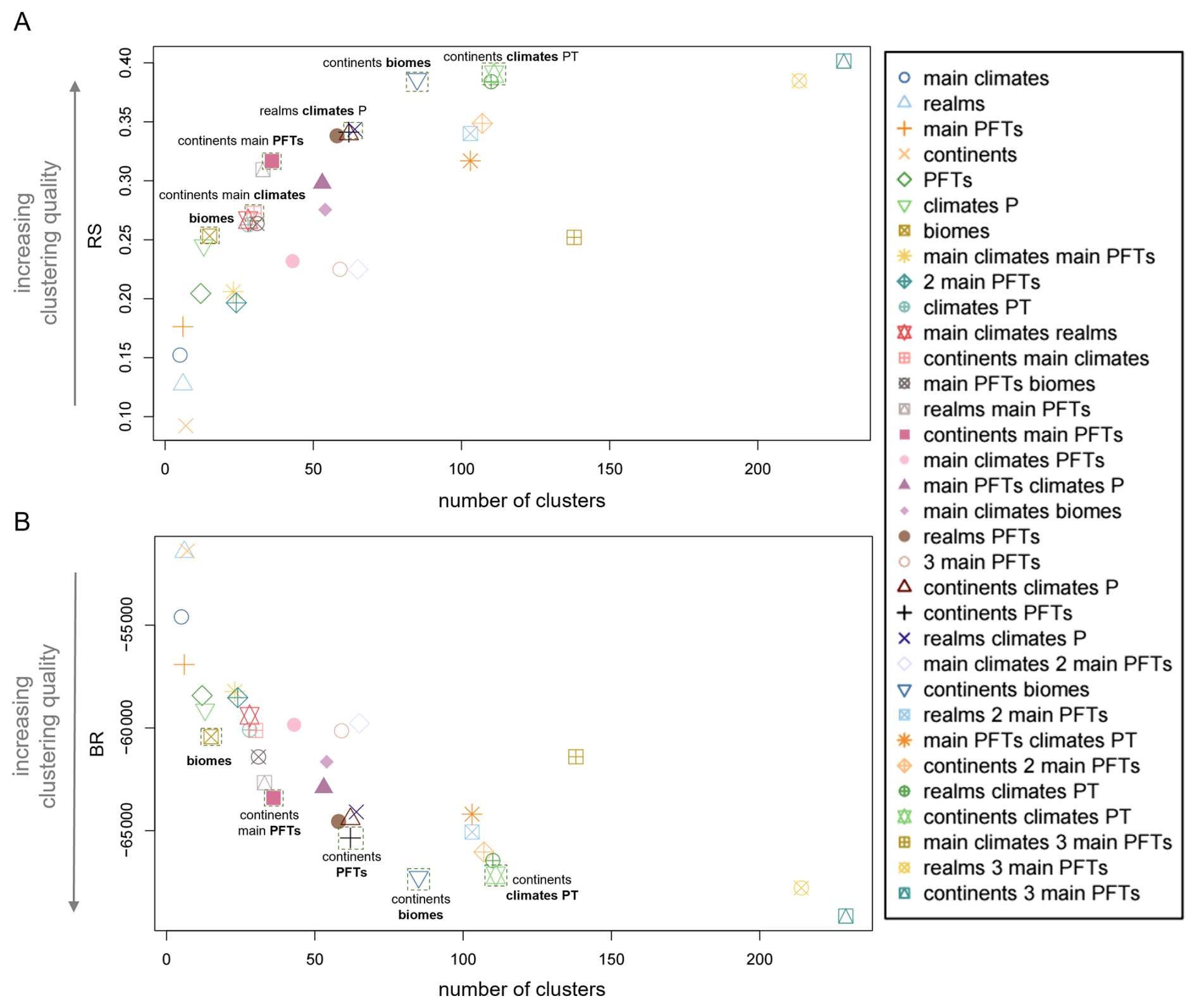
Figure E1Multivariate clustering performance of top-down partitions. (A) R-squared index (RS) and (B) Banfield-Raftery index (BR) of the 33 geographical, climatic and biological Earth partitions with respect to the magnitude of the effects of natural vegetation cover on surface water runoff and carbon storage, as well as the magnitude of the effects of change in carbon dioxide concentration on surface water runoff and natural vegetation cover. The partitions are sorted by their number of clusters and highlighted if they stand out in performance compared to partitions of similar number of clusters.
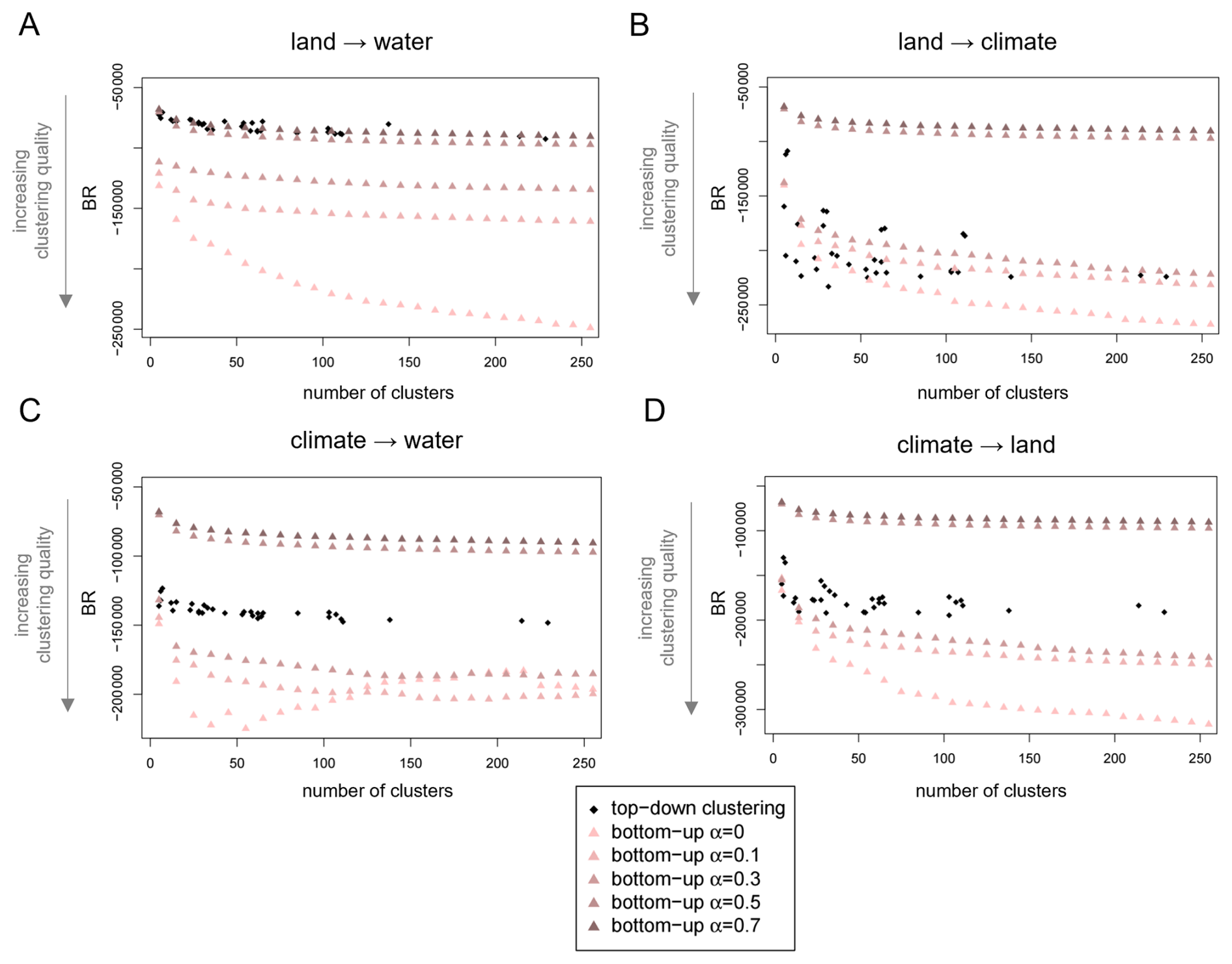
Figure F1Comparison of clustering performance of top-down and bottom-up partitions. Banfield-Raftery index (BR) of the 33 “top-down” geographical, climatic and biological Earth partitions and of the GeoClust “bottom-up” neighborhood-based partitions without spatial constraints (α=0), and with mixing parameters . Performance is evaluated separately based on the one-dimensional feature space of magnitude for (A) the effect of land on water, (B) land on climate, (C) climate on water, and (D) climate on land, respectively. The partitions are sorted by their number of clusters.
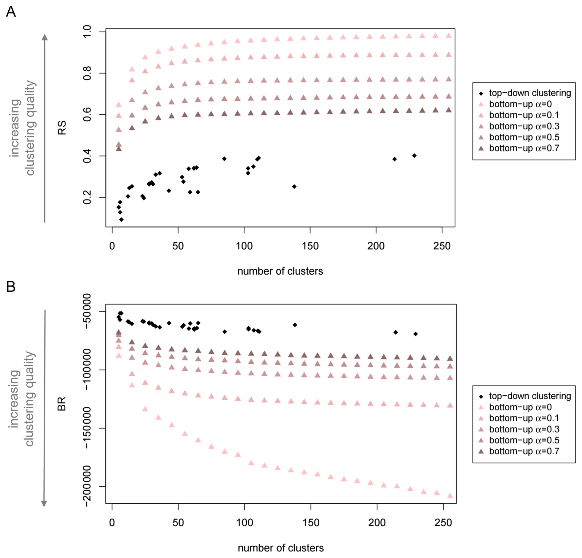
Figure F2Comparison of multivariate clustering performance of top-down and bottom-up partitions. (A) R-squared index (RS) and (B) Banfield-Raftery index (BR) of the 33 “top-down” geographical, climatic and biological Earth partitions and of the GeoClust “bottom-up” neighborhood-based partitions without spatial constraints (α=0), and for mixing parameters . The four-dimensional feature space consists of the magnitudes of the effects of natural vegetation cover on surface water runoff and carbon storage, as well as the magnitudes of the effects of change in carbon dioxide concentration on surface water runoff and natural vegetation cover. The partitions are sorted by their number of clusters.
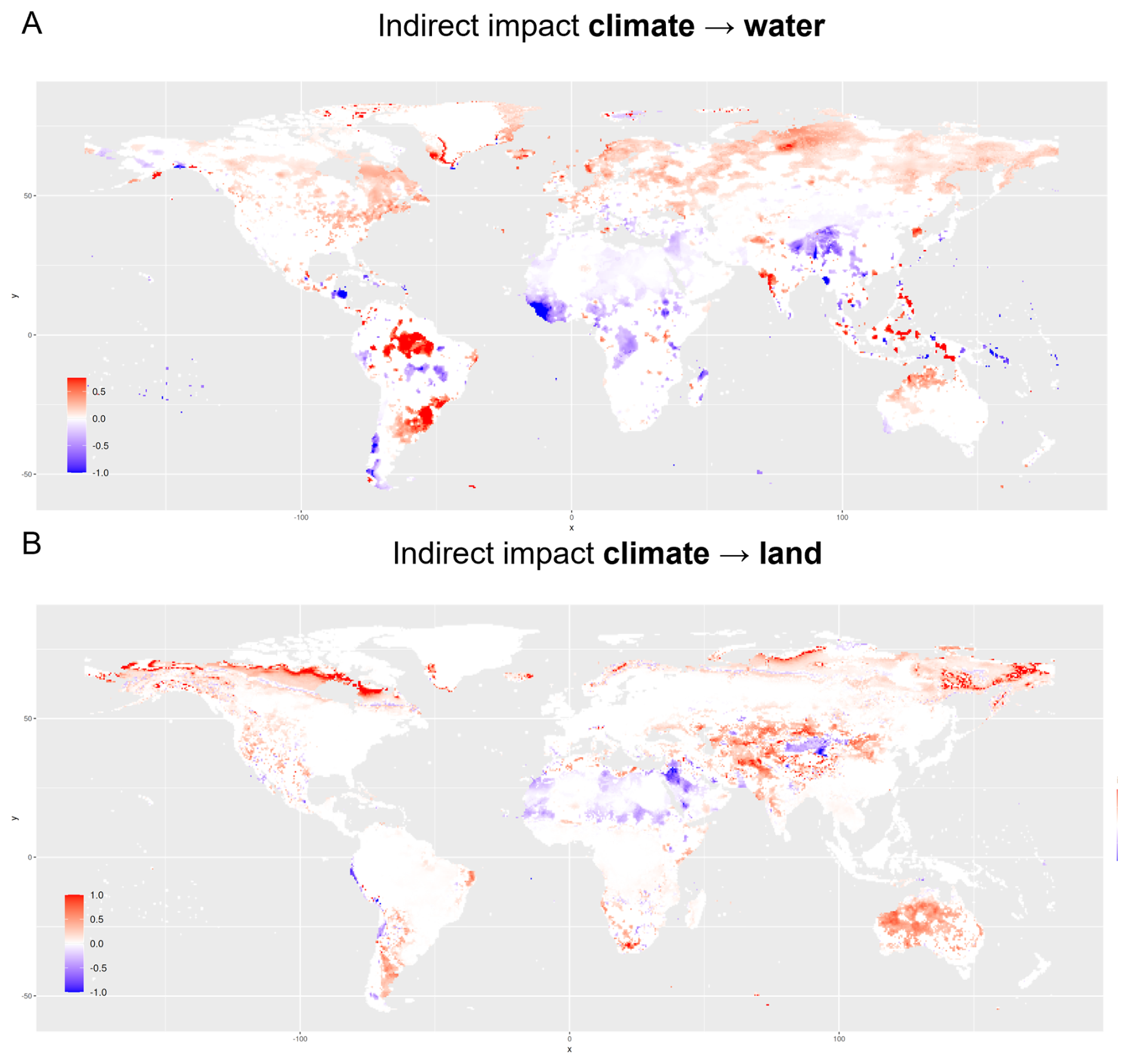
Figure G1Global pattern of indirect impacts of climate change on water and land. The maps display the rescaled magnitudes of the effects of changes in carbon dioxide concentration on (A) surface water and (B) natural vegetation cover. Positive effect size indicates that an increase in carbon dioxide concentration causes an increase in the respective other Earth system process. Analogously, negative effect size indicates that an increase in carbon dioxide concentration leads to a decrease in the other process. Note that for the sake of visibility, the color scale varies across effect types and directions and should therefore not be used for cross-comparisons.
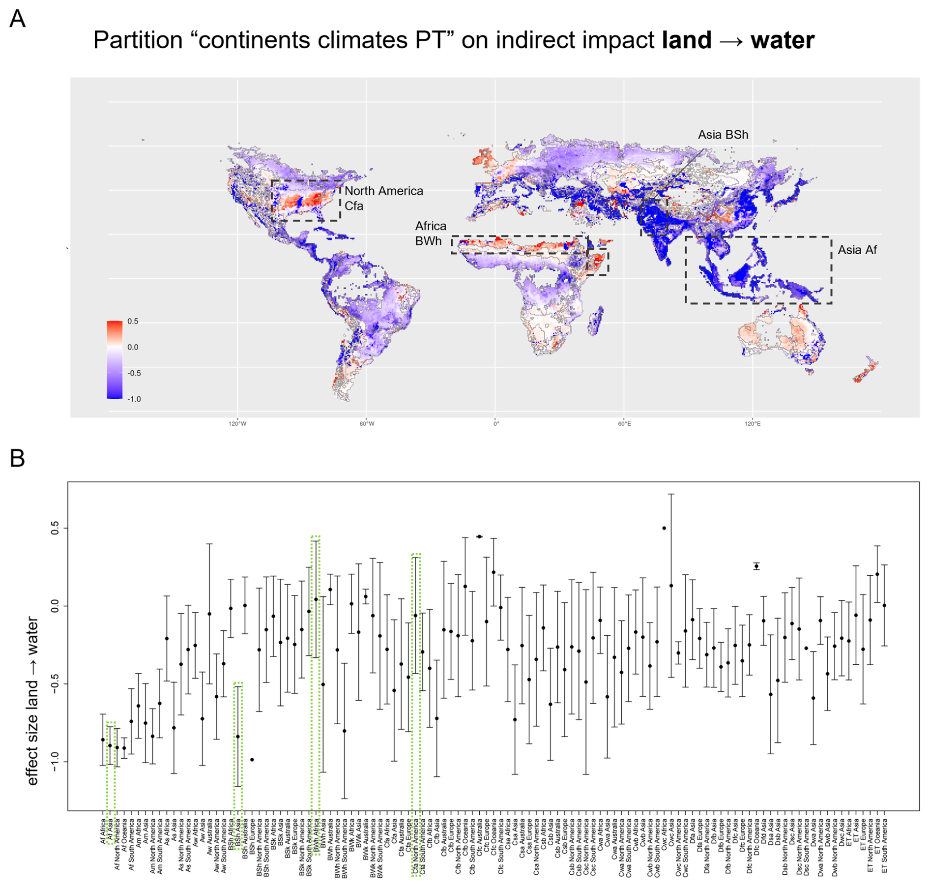
Figure H1Magnitude of the indirect impact of land use change on water with boundaries given by continent and Köppen-Geiger climate zone (climate PT). (A) Map showing the magnitude of the effect of change in natural vegetation cover on surface water runoff. Boundaries mark both continents and climates/precipitation. Four of the five clusters exhibiting the strongest negative impact are rainforests (Af). A strong positive effect size can be observed in the hot desert (BWh) of Africa. One cluster for which it is particularly apparent that the pattern of effect size is not well represented by an average value is the fully humid, hot summer region (Cfa) in eastern North America, indicating driving mechanisms beyond climate and precipitation. Here, the distinctive nature of the Mississippi River ecosystem is not reflected by the Köppen Geiger climatic boundaries. (B) Mean and standard deviations of the effect size within each cluster of the partition in (A). See Table B1 for the nomenclature of the climate zones. The same clusters are highlighted in panel (A) and panel (B).
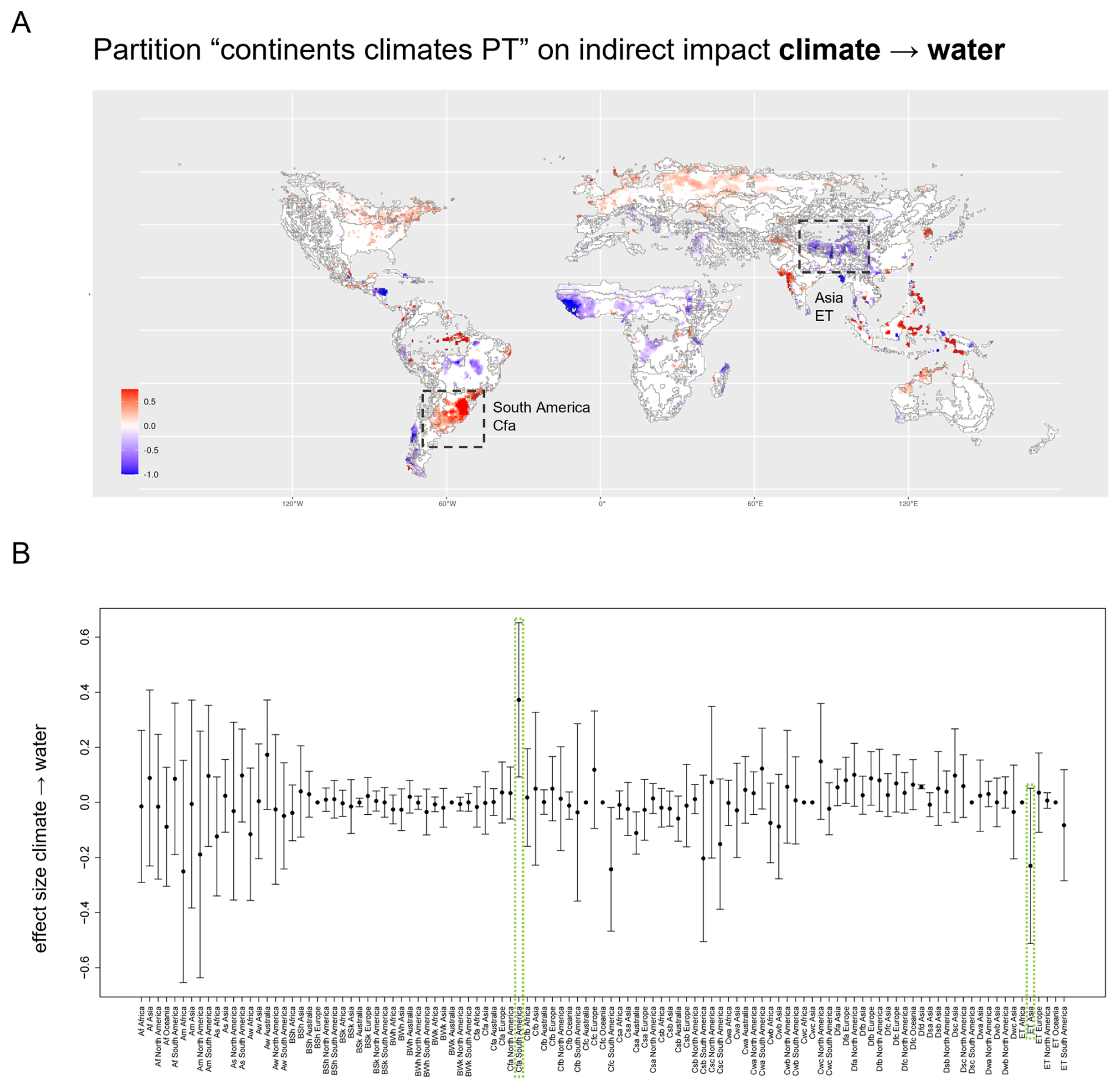
Figure H2Magnitude of the indirect impact of climate change on water with boundaries given by continent and Köppen-Geiger climate zone (climate PT). (A) Map showing the magnitude of the effect of change in carbon dioxide concentration on surface water runoff. Boundaries mark both continents and climates/precipitation. The effect is strongly positive in the fully humid, hot summer region of South America (Cfa). In contrast, the Asian tundra (ET) is characterized by a notable negative effect size. (B) Mean and standard deviations of the effect size within each cluster of the partition in (A). See Table B1 for the nomenclature of the climate zones. The same clusters are highlighted in panel (A) and panel (B).
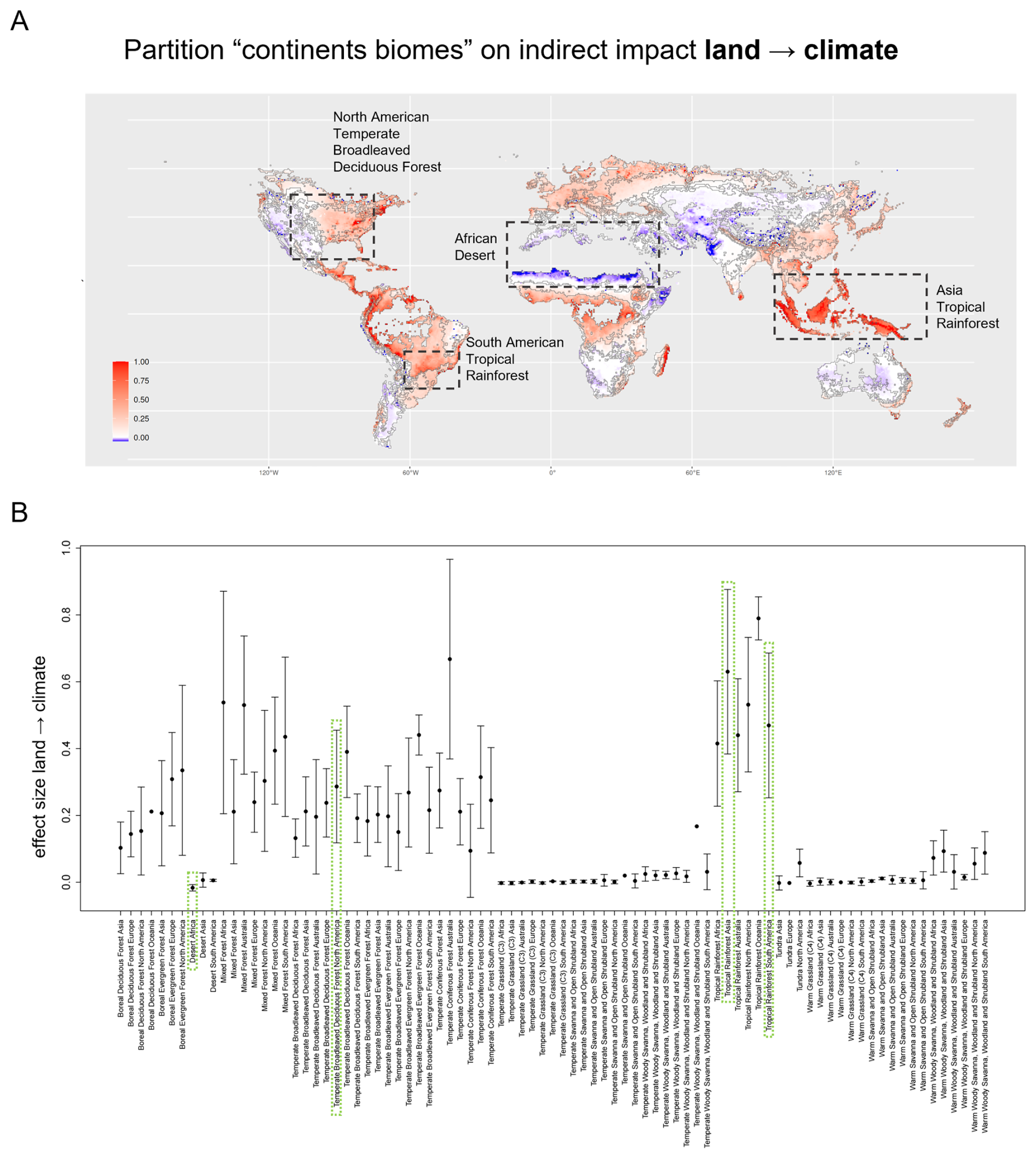
Figure H3Magnitude of the indirect impact of land use change on climate with boundaries given by continent and biome. (A) Map showing the magnitude of the effect of change in natural vegetation cover on carbon dioxide storage. Boundaries mark both continents and biomes. We observe an extensive high positive effect size in the Asian Tropical Rainforest. The reverse effect occurs in the African Desert, where a conversion to cropland apparently increases the carbon storage capacity of an area. This effect might be due to the natural vegetation occurring on cropland in between growing seasons. The boundaries of the North American Temperate Broad-leaved Deciduous Forest remarkably well separate areas of higher to moderate effect size from areas of little to no effect further westward. The border between the South American Rainforest and the Temperate Broad-leaved Deciduous Forest provides another example of an exact separation between regions of different levels of effect size. (B) Mean and standard deviations of the effect size within each cluster of the partition in (A). The same clusters are highlighted in panel (A) and panel (B).
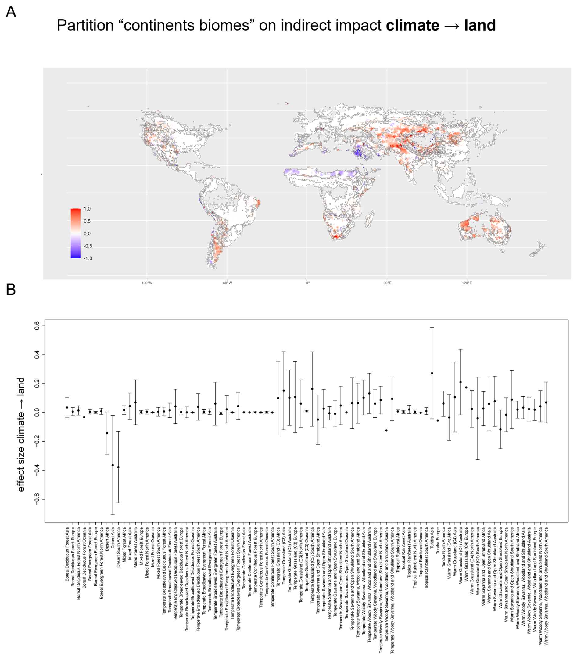
Figure H4Magnitude of the indirect impact of climate change on natural vegetation cover with boundaries given by continent and the two main plant functional types (2 main PFTs). (A) Map showing the magnitude of the effect of change in carbon dioxide storage on natural vegetation cover. Boundaries mark both realms and the two main plant functional types. Areas mentioned in the main text are highlighted. (B) Mean and standard deviations of the effect size within each cluster of the partition in (A).
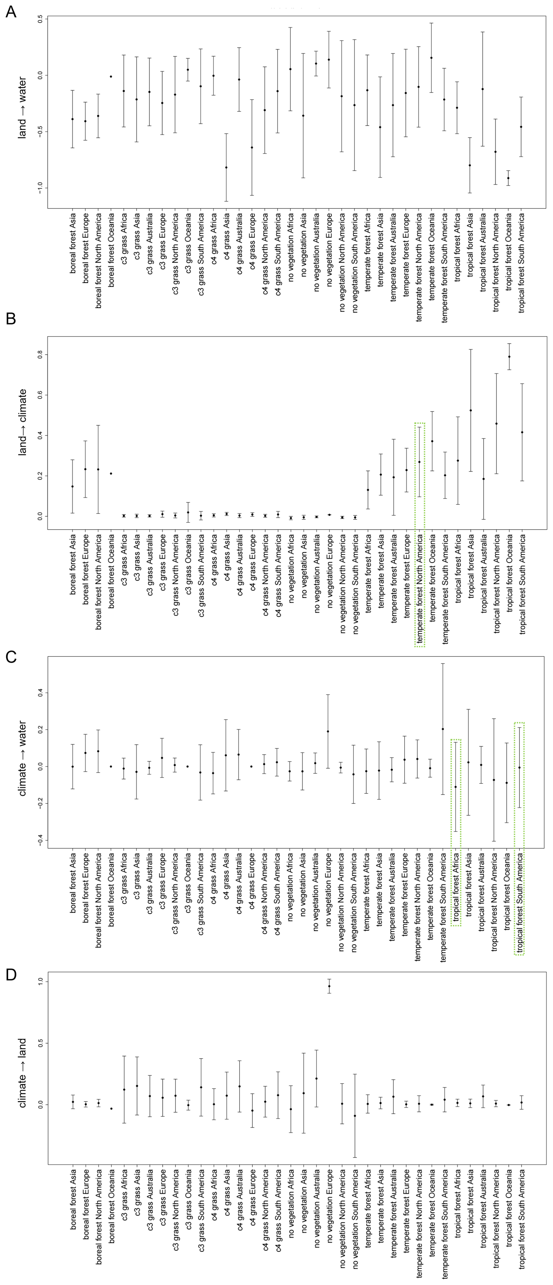
Figure I1Aggregations of effect size with respect to the clusters used by Lade et al. (2021b). Clusters are based on a distinction of both continent and dominant main plant functional type. Mean and standard deviation of effect size within each cluster for the effects of land use change on (A) surface water runoff and on (B) climate, as well as for the effects of climate change on (C) surface water runoff and (D) natural vegetation cover. The highlighted clusters are being discussed in the Results and Discussion section.
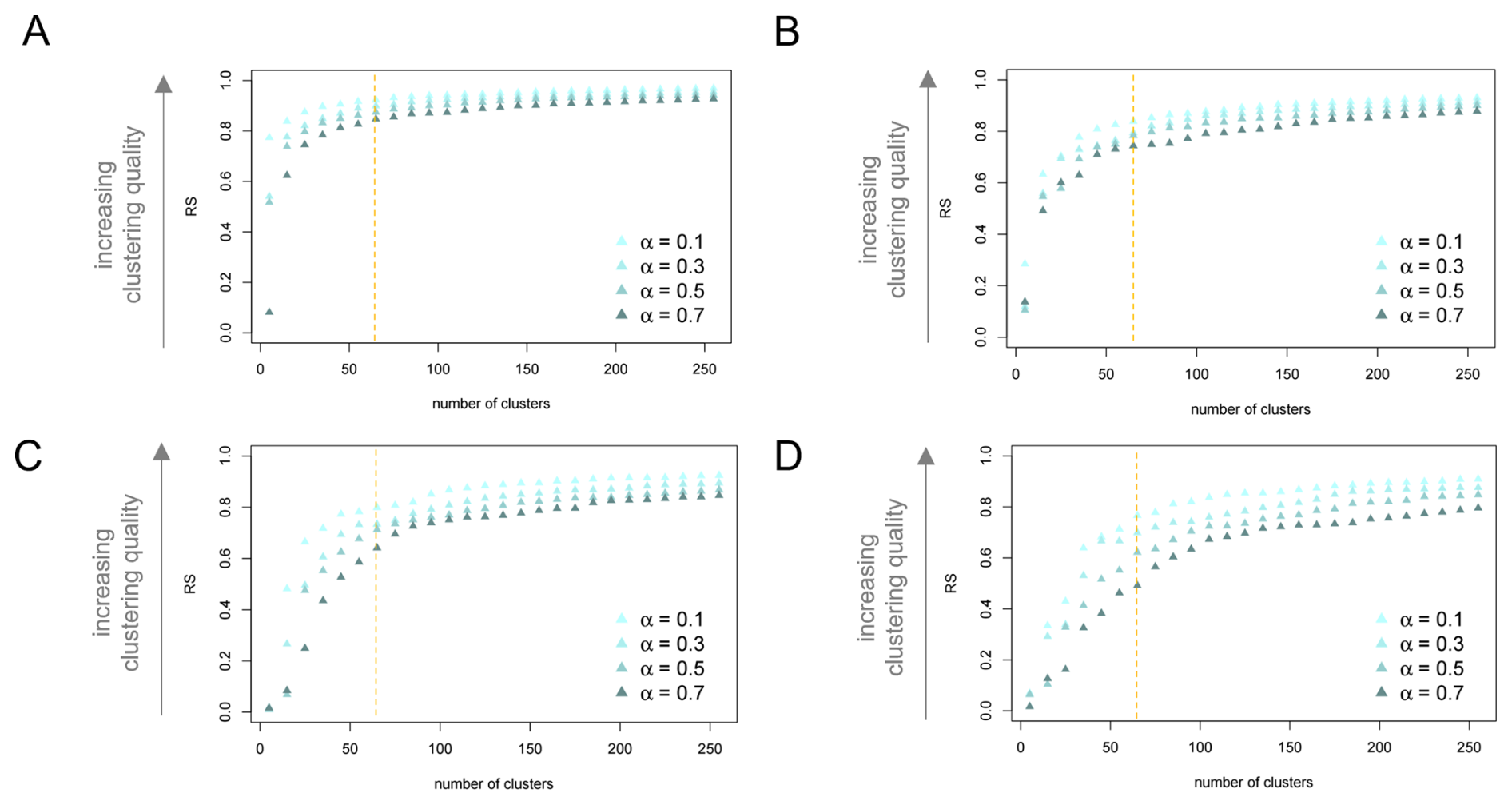
Figure J1Performance of distance-based bottom-up partitions by effect type and for varying mixing parameter α. R-squared index (RS) for the distance-based bottom-up partition generated by ClustGeo based on the univariate feature space of the effects of natural vegetation change on (A) surface water runoff and (B) carbon dioxide storage as well as for the effects of change in carbon dioxide concentration on (C) surface water runoff and (D) natural vegetation cover. Indices are displayed for partitions generated with mixing parameter . Partitions are ordered by their number of clusters. The dashed orange lines mark indices for the partition into 65 clusters, which we consider in more detail.
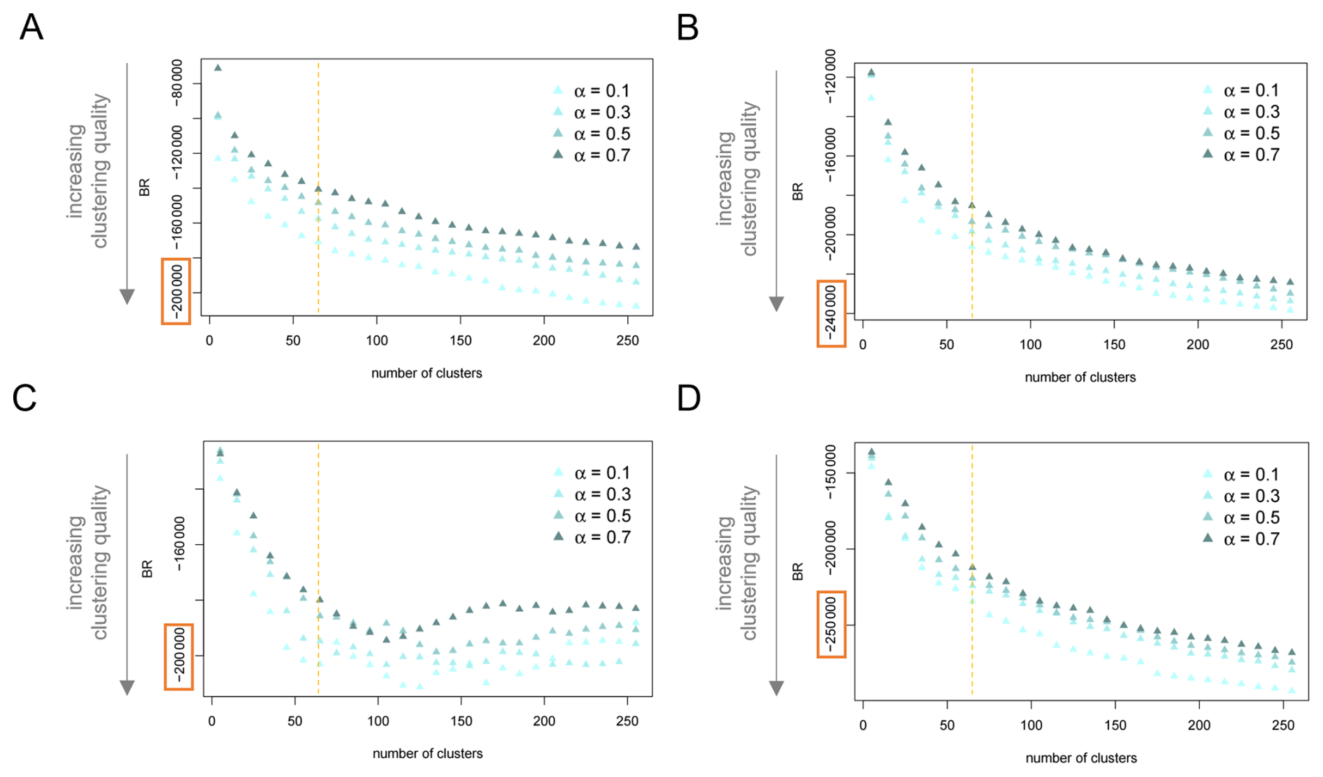
Figure J2Performance of distance-based bottom-up partitions by effect type and for varying mixing parameter α. Banfield-Raftery index (BR) for the distance-based bottom-up partition generated by ClustGeo based on the univariate feature space of the effects of natural vegetation change on (A) surface water runoff and (B) carbon dioxide storage as well as for the effects of change in carbon dioxide concentration on (C) surface water runoff and (D) natural vegetation cover. Indices are displayed for partitions generated with mixing parameter Partitions are ordered by their number of clusters. The dashed orange lines mark indices for the partition into 65 clusters, which we consider in more detail.
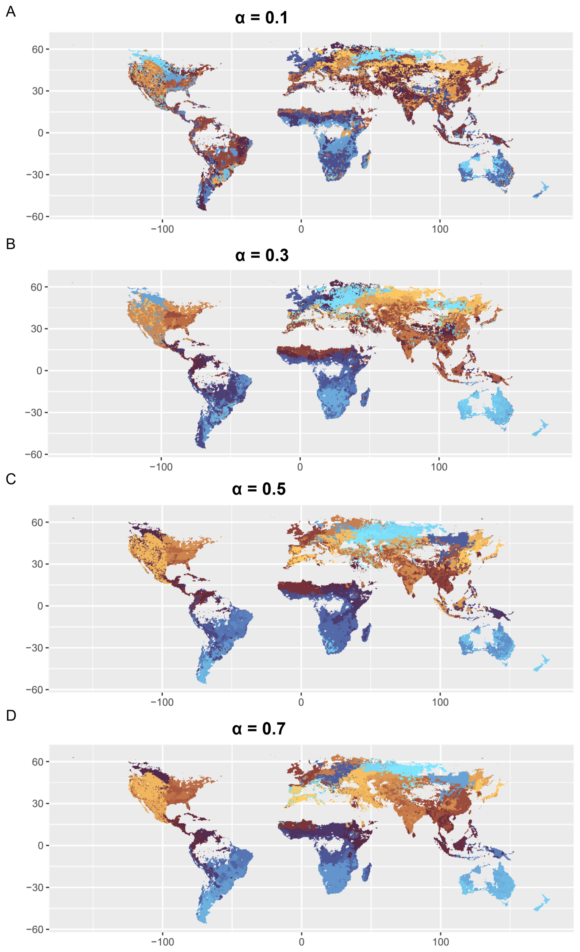
Figure K1World map of bottom-up impact zones for increasing levels of spatial cohesion. Global pattern of 65 clusters based on a geographic-distance-based constraint space and and the multidimensional feature space of magnitudes of the effects of land use change on water and climate and of the effects of climate change on water and land use. Generated via GeoClust with increasing level of spatial cohesion α=0.1 (A), α=0.3 (B), α=0.5 (C), α=0.7 (D).
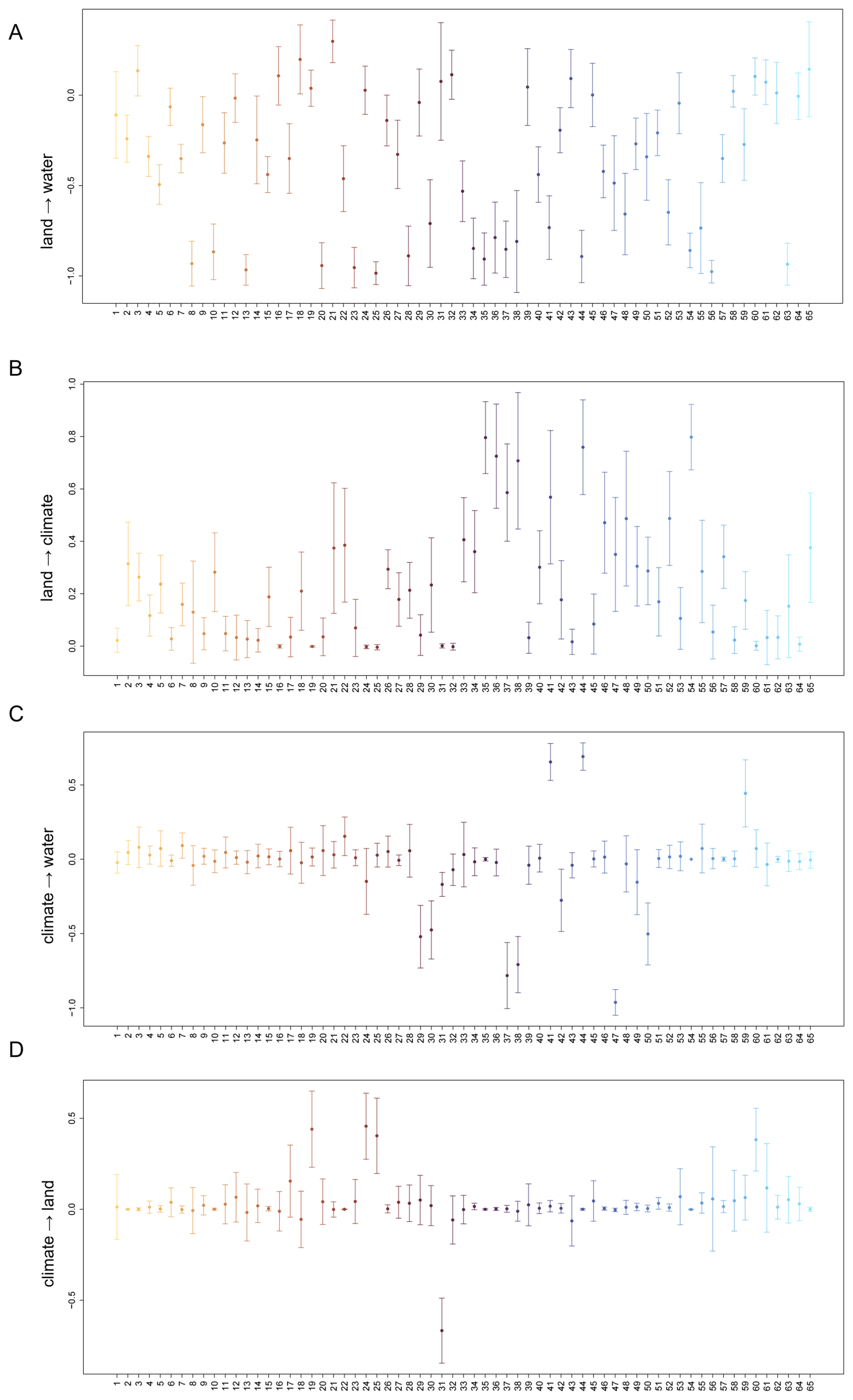
Figure K2Mean and standard deviation of effect sizes in the bottom-up impact zones. The partition into k=65 clusters was generated via GeoClust with mixing parameter α=0.7. Mean and standard deviation of effect sizes are displayed for the effects of land use change on (A) water and (B) climate and the effects of climate change on (C) water and (D) land use.
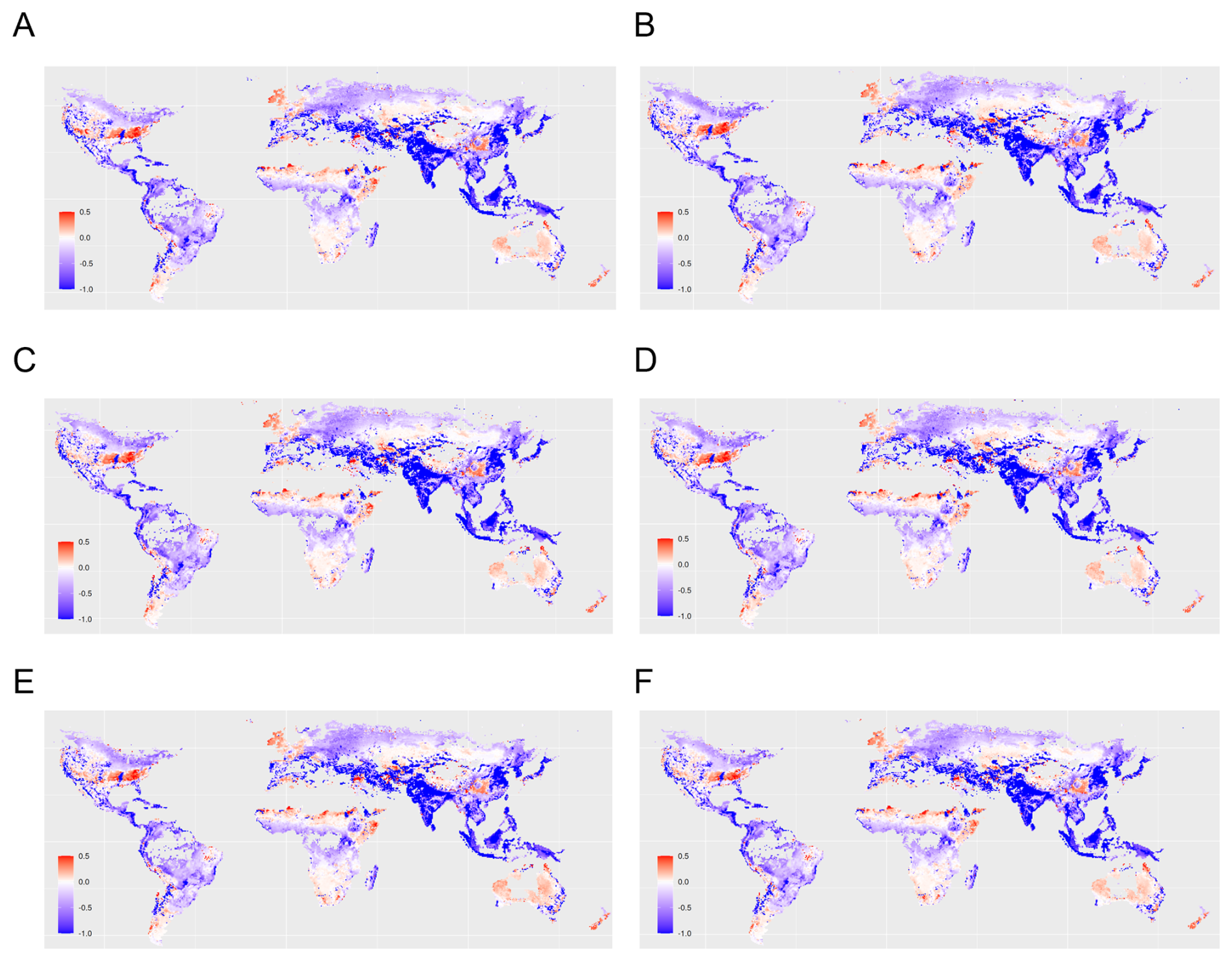
Figure L1Sensitivity of the global pattern of indirect impacts of land use change on surface water runoff. The maps display outputs based on the climate model (A) HadGEM2-AO (B) GFDL-CM3 (C) NorESM1-ME (D) GFDL-ESM2G (E) CanESM2 (F) MIROC-ESM. Positive effect size (red) indicates that an increase in one Earth system process (e.g., increased natural vegetation cover) causes an increase in another Earth system process (e.g., increased surface water runoff). Analogously, negative effect size (blue) indicates that an increase in one process leads to a decrease in another process.
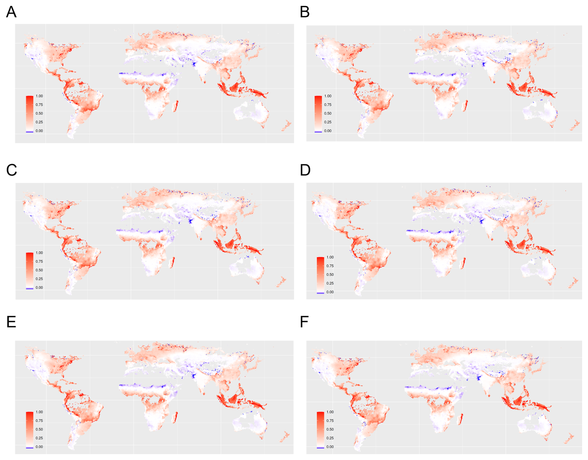
Figure L2Sensitivity of the global pattern of indirect impacts of land use change on carbon storage density. The maps display outputs based on the climate model (A) HadGEM2-AO (B) GFDL-CM3 (C) NorESM1-ME (D) GFDL-ESM2G (E) CanESM2 (F) MIROC-ESM. Positive effect size (red) indicates that an increase in one Earth system process (e.g., increased natural vegetation cover) causes an increase in another Earth system process (e.g., increased surface water runoff). Analogously, negative effect size (blue) indicates that an increase in one process leads to a decrease in another process.
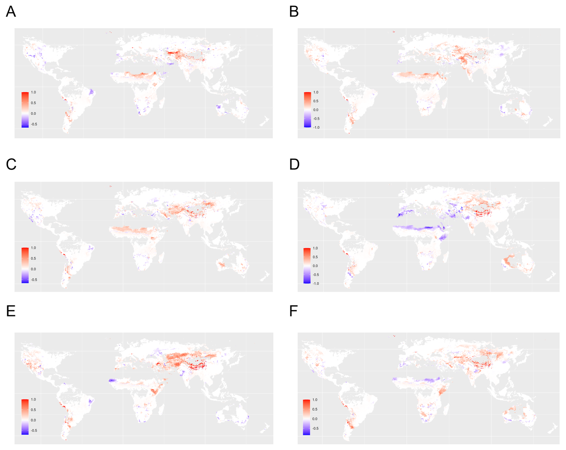
Figure L3Sensitivity of the global pattern of indirect impacts of climate change on surface water runoff. The maps display outputs based on the climate model (A) HadGEM2-AO (B) GFDL-CM3 (C) NorESM1-ME (D) GFDL-ESM2G (E) CanESM2 (F) MIROC-ESM. Positive effect size (red) indicates that an increase in one Earth system process (e.g., increased natural vegetation cover) causes an increase in another Earth system process (e.g., increased surface water runoff). Analogously, negative effect size (blue) indicates that an increase in one process leads to a decrease in another process.
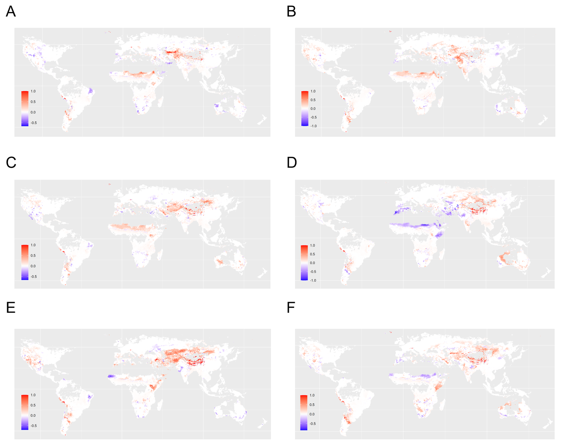
Figure L4Sensitivity of the global pattern of indirect impacts of climate change on natural vegetation cover. The maps display outputs based on the climate model (A) HadGEM2-AO (B) GFDL-CM3 (C) NorESM1-ME (D) GFDL-ESM2G (E) CanESM2 (F) MIROC-ESM. Positive effect size (red) indicates that an increase in one Earth system process (e.g., increased natural vegetation cover) causes an increase in another Earth system process (e.g., increased surface water runoff). Analogously, negative effect size (blue) indicates that an increase in one process leads to a decrease in another process.
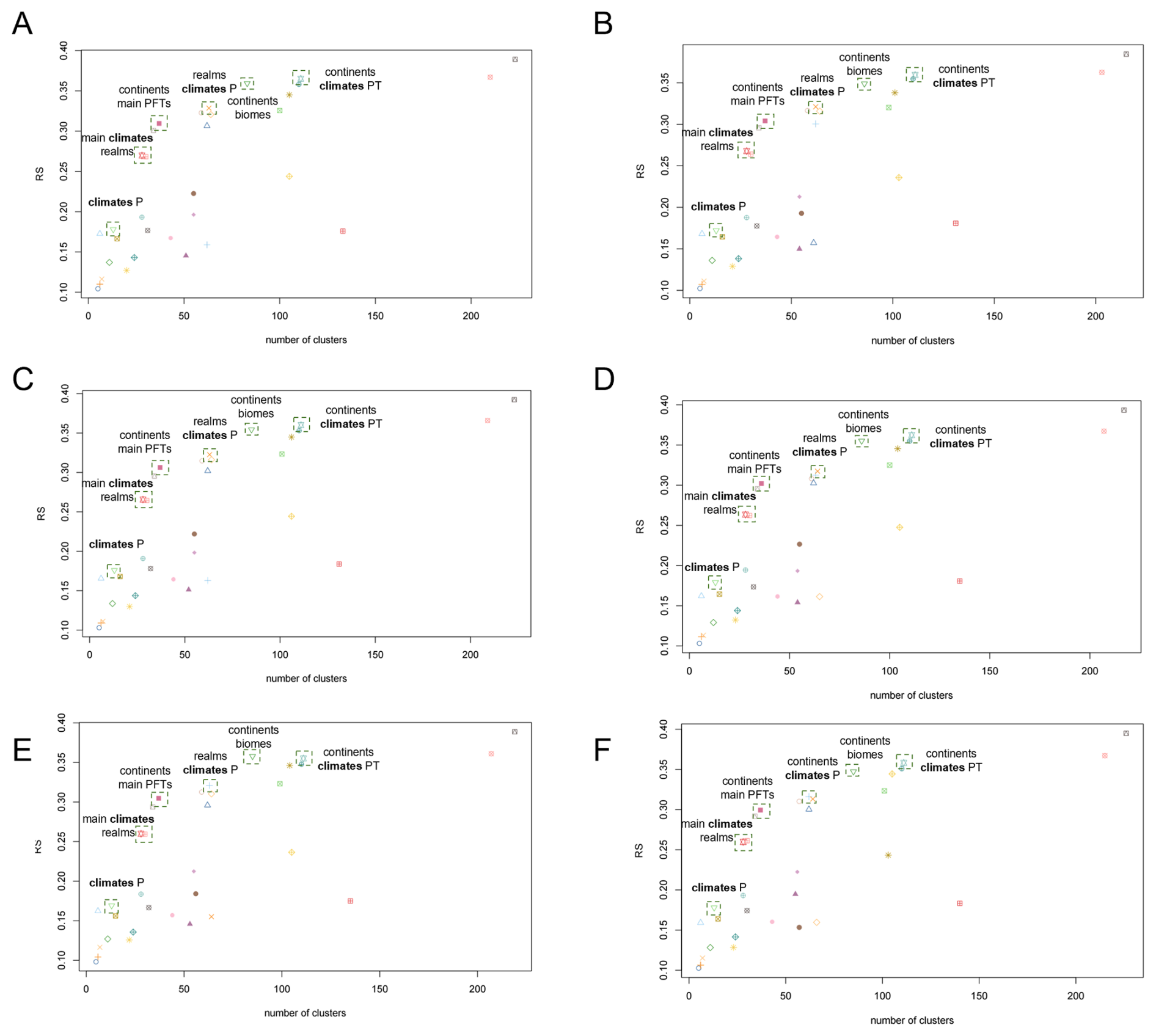
Figure M1Sensitivity of the performance of the RS index for top-down clustering for the effect of land use change on surface water runoff. The maps display outputs based on the climate model (A) HadGEM2-AO (B) GFDL-CM3 (C) NorESM1-ME (D) GFDL-ESM2G (E) CanESM2 (F) MIROC-ESM. Positive effect size (red) indicates that an increase in one Earth system process (e.g., increased natural vegetation cover) causes an increase in another Earth system process (e.g., increased surface water runoff). Analogously, negative effect size (blue) indicates that an increase in one process leads to a decrease in another process.
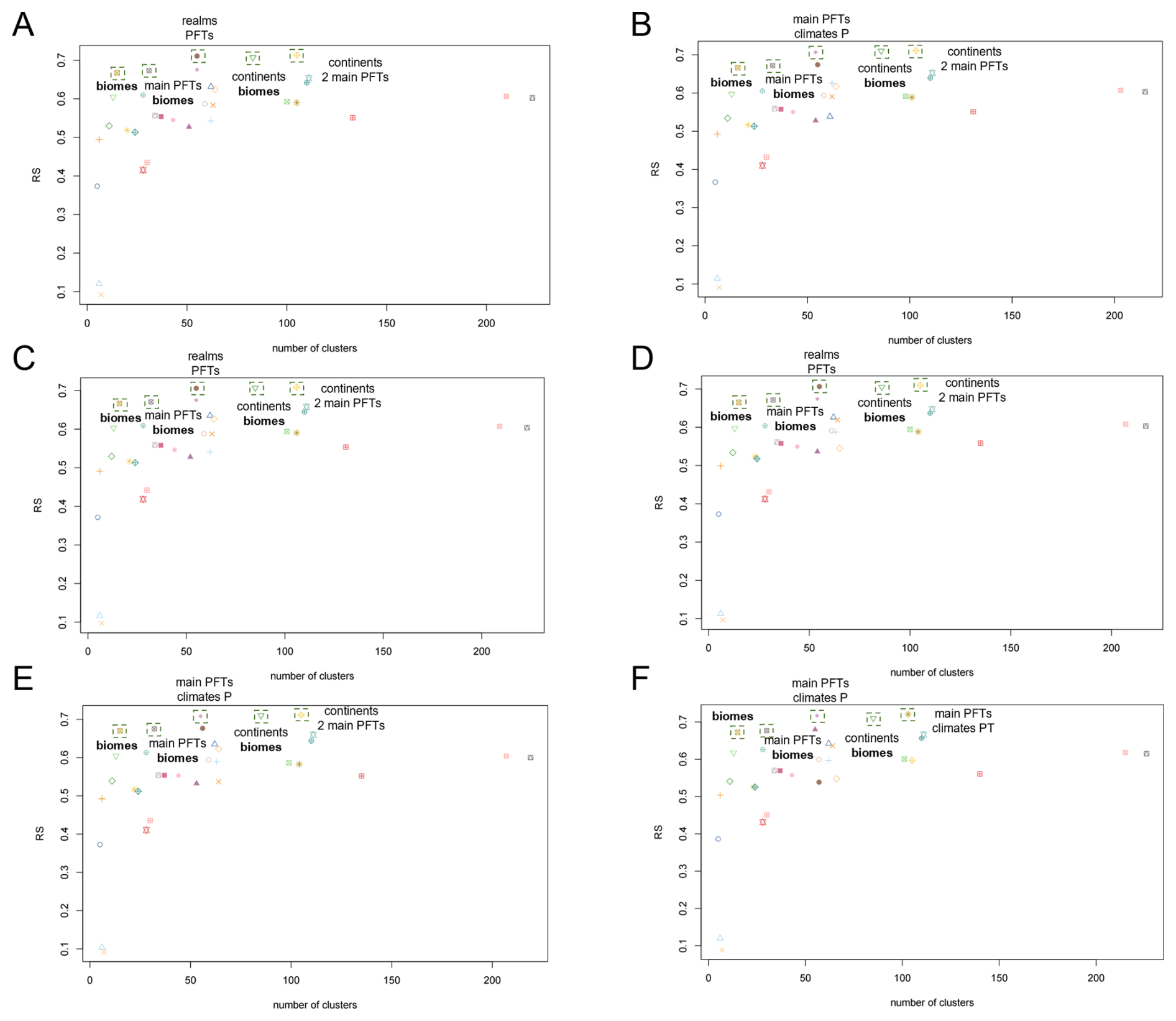
Figure M2Sensitivity of the performance of the RS index for top-down clustering for the effect of land use change on carbon storage density. The maps display outputs based on the climate model (A) HadGEM2-AO (B) GFDL-CM3 (C) NorESM1-ME (D) GFDL-ESM2G (E) CanESM2 (F) MIROC-ESM. Positive effect size (red) indicates that an increase in one Earth system process (e.g., increased natural vegetation cover) causes an increase in another Earth system process (e.g., increased surface water runoff). Analogously, negative effect size (blue) indicates that an increase in one process leads to a decrease in another process.
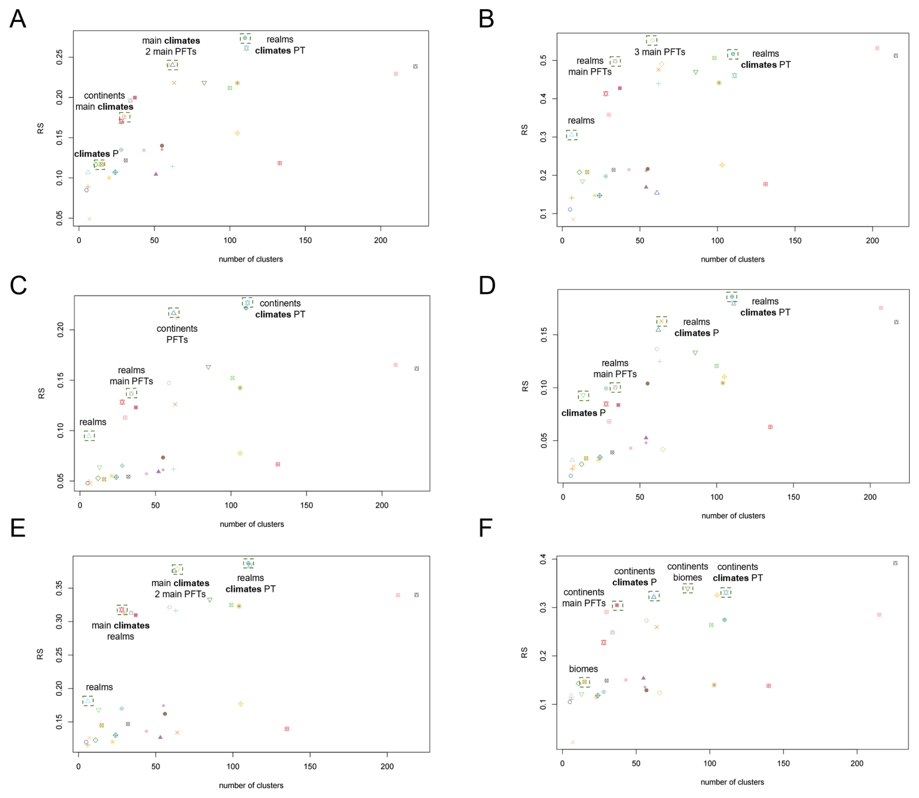
Figure M3Sensitivity of the performance of the RS index for top-down clustering for the effect of climate change on surface water runoff. The maps display outputs based on the climate model (A) HadGEM2-AO (B) GFDL-CM3 (C) NorESM1-ME (D) GFDL-ESM2G (E) CanESM2 (F) MIROC-ESM. Positive effect size (red) indicates that an increase in one Earth system process (e.g., increased natural vegetation cover) causes an increase in another Earth system process (e.g., increased surface water runoff). Analogously, negative effect size (blue) indicates that an increase in one process leads to a decrease in another process.
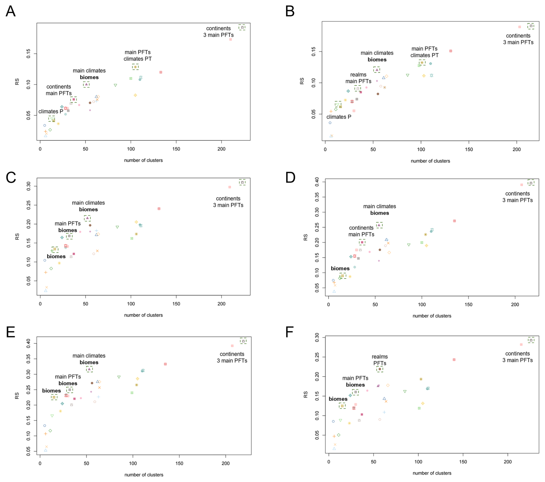
Figure M4Sensitivity of the performance of the RS index for top-down clustering for the effect of land use change on surface water runoff. The maps display outputs based on the climate model (A) HadGEM2-AO (B) GFDL-CM3 (C) NorESM1-ME (D) GFDL-ESM2G (E) CanESM2 (F) MIROC-ESM. Positive effect size (red) indicates that an increase in one Earth system process (e.g., increased natural vegetation cover) causes an increase in another Earth system process (e.g., increased surface water runoff). Analogously, negative effect size (blue) indicates that an increase in one process leads to a decrease in another process.
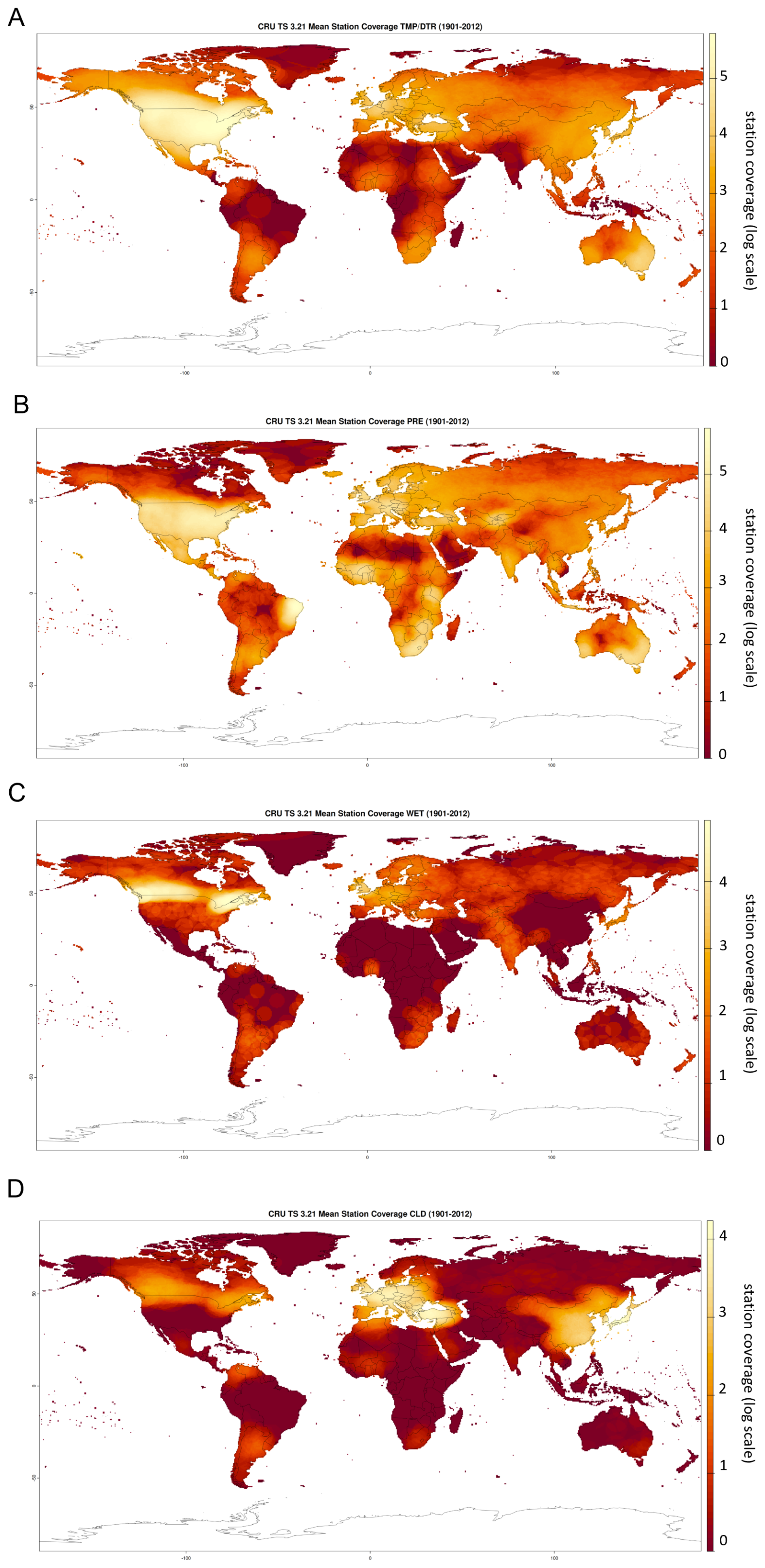
Figure N1Station coverage underlying the CRU TS3.21 dataset (Harris, 2013). The station cover of a grid cell at a point in time is being defined as the number of stations within the correlation decay distance of the cell that were reporting a valid value at that point in time. Maps display the log-scaled station cover per grid cell averaged across 1901–2012 for the variables of (A) mean temperature (TMP) and diurnal temperature range (DTR) combined, (B) total precipitation (PRE), (C) rainday counts (WET) and (D) cloud cover (CLD). See Harris et al. (2014) for more details on the computation of the station coverage.
Our results are based on the LPJmL simulation data by Lade et al. (2021a) (https://doi.org/10.5281/zenodo.4738009). The computation of the global station coverage uses the CRU TS3.21 dataset by Harris (2013) (https://doi.org/10.5285/D0E1585D-3417-485F-87AE-4FCECF10A992). The R code underlying our results is provided as Supplement to this manuscript.
The supplement related to this article is available online at https://doi.org/10.5194/esd-17-1719-2026-supplement.
Conceptualization: HZ, SJL, JCR; Software: HZ, CKGG, IF, NC; Analysis: HZ, SJL, JCR, CKGG; Writing (original draft): HZ; Writing (revision): HZ, SJL, JCR, CKGG, IF, NC.
At least one of the (co-)authors is a member of the editorial board of Earth System Dynamics. The peer-review process was guided by an independent editor, and the authors also have no other competing interests to declare.
Publisher's note: Copernicus Publications remains neutral with regard to jurisdictional claims made in the text, published maps, institutional affiliations, or any other geographical representation in this paper. The authors bear the ultimate responsibility for providing appropriate place names. Views expressed in the text are those of the authors and do not necessarily reflect the views of the publisher.
This article is part of the special issue “Earth resilience in the Anthropocene”. It is not associated with a conference.
HZ, JCR, IF, and NC received funding from the Swedish Research Council Formas (project 2023-00310). CKGG was funded by the Australian Government (Australian Research Council Discovery Project DP230101280). SJL was funded by the Australian Government (Australian Research Council Future Fellowship FT200100381).
The publication of this article was funded by the Swedish Research Council, Forte, Formas, and Vinnova.
This paper was edited by Nico Wunderling and reviewed by Shuchang Tang and Fabian Stenzel.
Betts, R., Boucher, O., Collins, M., Cox, P., Falloon, P., Gedney, N., Hemming, D., Huntingford, C., Jones, C., Sexton, D., and Webb, M.: Projected Increase in Continental Runoff Due to Plant Responses to Increasing Carbon Dioxide, Nature, 448, 1037–41, https://doi.org/10.1038/nature06045, 2007. a
Chavent, M., Kuentz-Simonet, V., Labenne, A., and Saracco, J.: ClustGeo: an R package for hierarchical clustering with spatial constraints, Computation. Stat., 33, 1799–1822, https://doi.org/10.1007/s00180-018-0791-1, 2018. a, b, c
Chen, J., Lei, C., Chu, H., Li, X., Torn, M., Wang, Y., Sciusco, P., and Robertson, G.: Overlooked cooling effects of albedo in terrestrial ecosystems, Environ. Res. Lett., 19, 093001, https://doi.org/10.1088/1748-9326/ad661d, 2024. a
Cramer, W., Bondeau, A., Woodward, I., Prentice, I., Betts, R., Brovkin, V., Cox, P., Fisher, V., Foley, J., Friend, A., Kucharik, C., Lomas, M., Ramankutty, N., Sitch, S., Smith, B., White, A., and Young-Molling, C.: Global response of terrestrial ecosystem structure and function to CO2 and climate change: Results from six dynamic global vegetation models, Glob. Change Biol., 7, 357–373, https://doi.org/10.1046/j.1365-2486.2001.00383.x, 2001. a
Dinerstein, E., Olson, D. P., Graham, D. J., Webster, A. L., Primm, S. A., Bookbinder, M. P., and Ledec, G. C.: A Conservation Assessment of the Terrestrial Ecoregions of Latin America and the Caribbean, Environ. Conserv., 23, 378–379, https://api.semanticscholar.org/CorpusID:131043914 (last access: 13 November 2026), 1995. a, b
Dinerstein, E., Olson, D., Joshi, A., Vynne, C., Burgess, N. D., Wikramanayake, E., Hahn, N., Palminteri, S., Hedao, P., Noss, R., Hansen, M., Locke, H., Ellis, E. C., Jones, B., Barber, C. V., Hayes, R., Kormos, C., Martin, V., Crist, E., Sechrest, W., Price, L., Baillie, J. E. M., Weeden, D., Suckling, K., Davis, C., Sizer, N., Moore, R., Thau, D., Birch, T., Potapov, P., Turubanova, S., Tyukavina, A., de Souza, N., Pintea, L., Brito, J. C., Llewellyn, O. A., Miller, A. G., Patzelt, A., Ghazanfar, S. A., Timberlake, J., Klöser, H., Shennan-Farpón, Y., Kindt, R., Lillesø, J.-P. B., van Breugel, P., Graudal, L., Voge, M., Al-Shammari, K. F., and Saleem, M.: Ecoregions2017 © Resolve, https://ecoregions.appspot.com/ (last access: 28 February 2025), 2017. a, b
Drüke, M., Lucht, W., von Bloh, W., Petri, S., Sakschewski, B., Tobian, A., Loriani, S., Schaphoff, S., Feulner, G., and Thonicke, K.: The long-term impact of transgressing planetary boundaries on biophysical atmosphere–land interactions, Earth Syst. Dynam., 15, 467–483, https://doi.org/10.5194/esd-15-467-2024, 2024. a
Guo, R., Chen, T., Chen, X., Yuan, W., Liu, S., He, B., Li, L., Wang, S., Hu, T., Yan, Q., Wei, X., and Dai, J.: Estimating Global GPP From the Plant Functional Type Perspective Using a Machine Learning Approach, J. Geophys. Res.-Biogeo., 128, e2022JG007100, https://doi.org/10.1029/2022JG007100, 2023. a
Gupta, J., Bai, X., Liverman, D. M., Rockström, J., Qin, D., and Stewart-Koste, B.: A just world on a safe planet: a Lancet Planetary Health–Earth Commission report on Earth-system boundaries, translations, and transformations, The Lancet Planetary Health, 8, https://doi.org/10.1016/S2542-5196(24)00042-1, 2024. a
Harris, I.: CRU TS3.21: Climatic Research Unit (CRU) Time-Series (TS) Version 3.21 of High Resolution Gridded Data of Month-by-month Variation in Climate (Jan. 1901–Dec. 2012), NCAS British Atmospheric Data Centre [data set], https://doi.org/10.5285/D0E1585D-3417-485F-87AE-4FCECF10A992, 2013. a, b
Harris, I., Jones, P., Osborn, T., and Lister, D.: Updated high-resolution grids of monthly climatic observations – the CRU TS3.10 Dataset, Int. J. Climatol., 34, 623–642, https://doi.org/10.1002/joc.3711, 2014. a, b, c, d
Hasler, N., Williams, C. A., Carrasco Denney, V., Ellis, P. W., Shrestha, S., Terasaki Hart, D. E., Wolff, N. H., Yeo, S., Crowther, T. W., Werden, L. K., and Cook-Patton, S. C.: Accounting for albedo change to identify climate-positive tree cover restoration, Nat. Commun., 15, 2275, https://doi.org/10.1038/s41467-024-46577-1, 2024. a
Ito, A. and Inatomi, M.: Water-Use Efficiency of the Terrestrial Biosphere: A Model Analysis Focusing on Interactions between the Global Carbon and Water Cycles, J. Hydrometeorol., 13, 681–694, https://doi.org/10.1175/JHM-D-10-05034.1, 2012. a
Jong, R., Schaepman, M., Furrer, R., de Bruin, S., and Verburg, P.: Spatial relationship between climatologies and changes in global vegetation activity, Glob. Change Biol., 19, https://doi.org/10.1111/gcb.12193, 2013. a
Koirala, S., Jung, M., Reichstein, M., de Graaf, I. E. M., Camps-Valls, G., Ichii, K., Papale, D., Ráduly, B., Schwalm, C. R., Tramontana, G., and Carvalhais, N.: Global distribution of groundwater-vegetation spatial covariation, Geophys. Res. Lett., 44, 4134–4142, https://doi.org/10.1002/2017GL072885, 2017. a
Kottek, M., Grieser, J., Beck, C., Rudolf, B., and Rubel, F.: World Map of the Köppen-Geiger Climate Classification Updated, Meteorol. Z., 15, 259–263, https://doi.org/10.1127/0941-2948/2006/0130, 2006. a, b
Kottek, M., Grieser, J., Beck, C., Rudolf, B., and Rubel, F.: World Map of the Köppen-Geiger climate classification updated, https://koeppen-geiger.vu-wien.ac.at/present.htm (last access: 28 February 2025), 2017. a, b
Lade, S., Steffen, W., Vries, W., Carpenter, S., Donges, J., Gerten, D., Hoff, H., Newbold, T., Richardson, K., and Rockström, J.: Human impacts on planetary boundaries amplified by Earth system interactions, Nature Sustainability, 3, 119–128, https://doi.org/10.1038/s41893-019-0454-4, 2020. a
Lade, S. J., Fetzer, I., Cornell, S. E., and Crona, B.: Prototype Earth system impact metric: code and data, Zenodo [code and data set], https://doi.org/10.5281/zenodo.4738009, 2021a. a, b
Lade, S. J., Fetzer, I., Cornell, S. E., and Crona, B.: A prototype Earth system impact metric that accounts for cross-scale interactions, Environ. Res. Lett., 16, 115005, https://doi.org/10.1088/1748-9326/ac2db1, 2021b. a, b, c, d, e, f, g, h, i, j, k, l, m
Luo, Y., Gerten, D., le Maire, G., Parton, W., Weng, E., Zhou, X., Keough, C., Beier, C., Ciais, P., Cramer, W., Dukes, J., Emmett, B., Hanson, P., Knapp, A., Linder, S., Nepstad, D., and Rustad, L.: Modeled Interactive Effects of Precipitation, temperature, and [CO2] on Ecosystem Carbon and Water Dynamics in Different Climatic Zones, Glob. Change Biol., 14, 1986–1999, https://doi.org/10.1111/j.1365-2486.2008.01629.x, 2008. a
Mohamed, A., DeClerck, F., Verburg, P. H., Obura, D., Abrams, J. F., Zafra-Calvo, N., Rocha, J., Estrada-Carmona, N., Fremier, A., Jones, S. K., Meier, I. C., and Stewart-Koster, B.: Securing Nature’s Contributions to People requires at least 20 %–25 % (semi-)natural habitat in human-modified landscapes, One Earth, 7, 59–71, https://doi.org/10.1016/j.oneear.2023.12.008, 2024. a
Ostberg, S., Lucht, W., Schaphoff, S., and Gerten, D.: Critical impacts of global warming on land ecosystems, Earth Syst. Dynam., 4, 347–357, https://doi.org/10.5194/esd-4-347-2013, 2013. a, b
Page, J., Abramowitz, G., De Kauwe, M., and Pitman, A.: Are Plant Functional Types Fit for Purpose?, Geophys. Res. Lett., 51, https://doi.org/10.1029/2023GL104962, 2023. a, b
Piao, S., Friedlingstein, P., Ciais, P., de Noblet-Ducoudré, N., Labat, D., and Zaehle, S.: Changes in climate and land use have a larger direct impact than rising CO2 on global river runoff trends, P. Natl. Acad. Sci. USA, 104, 15242–15247, https://doi.org/10.1073/pnas.0707213104, 2007. a, b, c, d
Priesner, J., Hötten, D., Schötz, D., Tietjen, B., Gelbrecht, M., Billing, M., Stenzel, F., and Thonicke, K.: Reducing the computational cost of dynamic global vegetation models with locally weighted hierarchical clustering, The European Physical Journal Special Topics, https://doi.org/10.1140/epjs/s11734-026-02526-1 , 2026. a
Richardson, K., Steffen, W., Lucht, W., Bendtsen, J., Cornell, S. E., Donges, J. F., Drüke, M., Fetzer, I., Bala, G., von Bloh, W., Feulner, G., Fiedler, S., Gerten, D., Gleeson, T., Hofmann, M., Huiskamp, W., Kummu, M., Mohan, C., Nogués-Bravo, D., Petri, S., Porkka, M., Rahmstorf, S., Schaphoff, S., Thonicke, K., Tobian, A., Virkki, V., Wang-Erlandsson, L., Weber, L., and Rockström, J.: Earth beyond six of nine planetary boundaries, Science Advances, 9, eadh2458, https://doi.org/10.1126/sciadv.adh2458, 2023. a
Runge, J., Bathiany, S., Bollt, E., Camps-Valls, G., Coumou, D., Deyle, E., Glymour, D., Kretschmer, M., Mahecha, M., Muñoz-Marí, J., van Nes, E., Peters, J., Quax, R., Reichstein, M., Scheffer, M., Schölkopf, B., Spirtes, P., Sugihara, G., Su, J., Zhang, K., and Zscheischler, J.: Inferring causation from time series in Earth system sciences, Nat. Commun., 10, 2553, https://doi.org/10.1038/s41467-019-10105-3, 2019. a
Schaphoff, S., von Bloh, W., Rammig, A., Thonicke, K., Biemans, H., Forkel, M., Gerten, D., Heinke, J., Jägermeyr, J., Langerwisch, F., Lucht, W., Rolinski, S., Waha, K., Ostberg, S., Wirth, S. B., Fader, M., Drüke, M., Jans, Y., Lutz, F., Herzfeld, T., Minoli, S., Porwollik, V., Stehfest, E., de Waal, L., Beringer (Erbrecht), T., Rost (Jachner), S., Gumpenberger, M., Heyder, U., Werner, C., Braun, J., Breier, J., Stenzel, F., Mathesius, S., Hemmen, M., Billing, M., Oberhagemann, L., Sakschewski, B., Hötten, D., and Müller, C.: compilation_of_land_use_datasets - PIK-LPJmL/LPJmL GitHub Wiki, GitHub [code], https://github-wiki-see.page/m/PIK-LPJmL/LPJmL/wiki/compilation_of_land_use_datasets (last access: 18 November 2026), 2018a. a
Schaphoff, S., von Bloh, W., Rammig, A., Thonicke, K., Biemans, H., Forkel, M., Gerten, D., Heinke, J., Jägermeyr, J., Knauer, J., Langerwisch, F., Lucht, W., Müller, C., Rolinski, S., and Waha, K.: LPJmL4 – a dynamic global vegetation model with managed land – Part 1: Model description, Geosci. Model Dev., 11, 1343–1375, https://doi.org/10.5194/gmd-11-1343-2018, 2018b. a, b
Sterling, S., Ducharne, A., and Polcher, J.: The impact of global land-cover change on the terrestrial water cycle, Nat. Clim. Change, 3, 385–390, https://doi.org/10.1038/nclimate1690, 2013. a, b, c
Terrer, C., Jackson, R. B., Prentice, I. C., Keenan, T. F., Kaiser, C., Vicca, S., Fisher, J. B., Reich, P. B., Stocker, B. D., Hungate, B. A., Peñuelas, J., McCallum, I., Soudzilovskaia, N. A., Cernusak, L. A., Talhelm, A. F., Van Sundert, K., Piao, S., Newton, P. C. D., Hovenden, M. J., Blumenthal, D. M., Liu, Y. Y., Müller, C., Winter, K., Field, C. B., Viechtbauer, W., Van Lissa, C. J., Hoosbeek, M. R., Watanabe, M., Koike, T., Leshyk, V. O., Wayne Polley, H., and Franklin, O.: Nitrogen and phosphorus constrain the CO2 fertilization of global plant biomass, Nat. Clim. Change, 9, 684–689, https://doi.org/10.1038/s41558-019-0545-2, 2019. a
Tobian, A., Gerten, D., Fetzer, I., Schaphoff, S., Andersen, L., Cornell, S., and Rockström, J.: Climate change critically affects the status of the land-system change planetary boundary, Environ. Res. Lett., 19, https://doi.org/10.1088/1748-9326/ad40c2, 2024. a
Todeschini, R., Ballabio, D., Termopoli, V., and Consonni, V.: Extended multivariate comparison of 68 cluster validity indices. A review, Chemometr. Intell. Lab., 251, 105117, https://doi.org/10.1016/j.chemolab.2024.105117, 2024. a, b
Trewin, B.: Assessing Internal Variability of Global Mean Surface Temperature From Observational Data and Implications for Reaching Key Thresholds, J. Geophys. Res.-Atmos., 127, e2022JD036747, https://doi.org/10.1029/2022JD036747, 2022. a
Udvardy, M.: A Classification of the Biogeographical Provinces of the World, International Union for Conservation of Nature and Natural Resources, https://portals.iucn.org/library/sites/library/files/documents/OP-018.pdf (last access: 13 November 2026), 1975. a
Zhou, S., Yu, B., Lintner, B., Findell, K., and Zhang, Y.: Projected increase in global runoff dominated by land surface changes, Nat. Clim. Change, 13, 442–449, https://doi.org/10.1038/s41558-023-01659-8, 2023. a, b, c, d, e, f, g
- Abstract
- Introduction
- Data and methods
- Results and Discussion
- Conclusions
- Appendix A: Natural Earth partitions
- Appendix B: Köppen Geiger classification scheme
- Appendix C: Spatially resolved maps of indirect impacts
- Appendix D: The BR index for top-down clustering by effect type
- Appendix E: Multivariate cluster validity indices for top-down clustering
- Appendix F: Comparison of cluster validity indices for top-down and bottom-up clustering
- Appendix G: World maps of effects of climate change
- Appendix H: Standard deviations in top-down partitions
- Appendix I: Aggregation of effect size by continent and main plant functional type
- Appendix J: Cluster validity indices for distance-based bottom-up clustering by effect type
- Appendix K: Distance-based bottom-up partitions for varying levels of spatial cohesion
- Appendix L: Sensitivity analysis: World maps of indirect impacts
- Appendix M: Sensitivity analysis: The RS index for top-down clustering by effect type
- Appendix N: Station coverage of the CRU TS3.21 dataset
- Code and data availability
- Author contributions
- Competing interests
- Disclaimer
- Special issue statement
- Financial support
- Review statement
- References
- Supplement
- Abstract
- Introduction
- Data and methods
- Results and Discussion
- Conclusions
- Appendix A: Natural Earth partitions
- Appendix B: Köppen Geiger classification scheme
- Appendix C: Spatially resolved maps of indirect impacts
- Appendix D: The BR index for top-down clustering by effect type
- Appendix E: Multivariate cluster validity indices for top-down clustering
- Appendix F: Comparison of cluster validity indices for top-down and bottom-up clustering
- Appendix G: World maps of effects of climate change
- Appendix H: Standard deviations in top-down partitions
- Appendix I: Aggregation of effect size by continent and main plant functional type
- Appendix J: Cluster validity indices for distance-based bottom-up clustering by effect type
- Appendix K: Distance-based bottom-up partitions for varying levels of spatial cohesion
- Appendix L: Sensitivity analysis: World maps of indirect impacts
- Appendix M: Sensitivity analysis: The RS index for top-down clustering by effect type
- Appendix N: Station coverage of the CRU TS3.21 dataset
- Code and data availability
- Author contributions
- Competing interests
- Disclaimer
- Special issue statement
- Financial support
- Review statement
- References
- Supplement