Simulating the impact of an AMOC weakening on the Antarctic Ice Sheet using a coupled climate and ice-sheet model

Climate model studies show that a shutdown of the Atlantic Meridional Overturning Circulation (AMOC) reduces northward heat transport into the North Atlantic, which causes an accumulation of heat in the South Atlantic Ocean. The Antarctic Ice Sheet meanwhile has been shown to be particularly susceptible to temperature changes in ocean water flowing into the cavities near ice-shelf grounding lines. How AMOC-induced modulation of inter-hemispheric heat transport could influence the present-day state of the Antarctic Ice Sheet via a southward propagation of warm anomalies is little studied. However, interactions between AMOC and the West Antarctic Ice Sheet are highly relevant, because both systems are classified as climate tipping elements, which can trigger irreversible changes in the Earth system.

In this study we simulate a shutdown of the AMOC, induced by artificial freshwater input to the North Atlantic, in a global climate model interactively coupled to an ice-sheet model for Antarctica. In line with previous studies, an AMOC shutdown causes increased sea-surface temperatures in the Southern Hemisphere along with a small shift in the mid-latitude westerlies. However, Southern Ocean subsurface temperatures, which drive basal melt in Antarctica, do not change in most regions along the Antarctic margin for the first eight centuries post AMOC shut down. Therefore, we do not find a change in the total Antarctic Ice volume in this time span. At later times, this is followed by a shift towards stronger Ross Sea convection, causing negative subsurface temperature anomalies of −1.4 °C on average. This cooling decreases basal melt in Antarctica, however increased calving balances the ice mass change. Even though our approach is simplified as the coupling is limited to the ocean-ice interface and results might be partly impacted by artificial freshwater hosing/forcing, this study is an important first step to quantitatively investigate Earth-system stability across both hemispheres in coupled climate–ice-sheet models.

1 Introduction

The Atlantic Meridional Overturning Circulation (AMOC) is considered a tipping element of the Earth system, which can undergo significant and often irreversible changes once a critical threshold is crossed (Manabe and Ronald, 1988; Rahmstorf et al., 2005; McKay et al., 2022). Therefore, under changing climate conditions such as increased global mean surface temperature or enhanced North Atlantic freshwater input due to increased precipitation or runoff/ice-sheet discharge, the AMOC could substantially weaken or shut down. As part of the global thermohaline ocean circulation, the AMOC plays a key role in transporting heat from the Southern to the Northern Hemisphere (Rahmstorf, 2002; Kuhlbrodt et al., 2007; Feulner et al., 2013) and is thereby crucial for global climate regimes (Vellinga and Wood, 2002; Knutti et al., 2004; Stouffer et al., 2006; Timmermann et al., 2007; Jackson and Wood, 2018) and in particular, present-day climate conditions in Europe (Jackson et al., 2015; Meccia et al., 2023). Several studies analysing existing observational data of the AMOC strength since 2004 show a downward trend (Smeed et al., 2018; Mishonov et al., 2024; Xing et al., 2026). While there are studies based on other indicators such as sea-surface temperature or climate proxy records (Dima and Lohmann, 2010; Caesar et al., 2021) that are able to reproduce this trend, others suggest no significant change (Terhaar et al., 2025) or that natural variability has dominated any signal (Latif et al., 2022). Suggested drivers of a decrease in AMOC strength since 2004 are increasing freshwater input in the North Atlantic due to more precipitation, sea-ice loss, as well as melt water from the Greenland ice sheet (Caesar et al., 2018). Climate projections using different state-of-the-art climate models confirm a continuing slowdown of the circulation at least until 2100 (IPCC AR6 WG1 Ch. 9.2.3.1, Fox-Kemper et al., 2021; Golledge et al., 2019; Gierz et al., 2015), which happens mainly due to changes in surface heat fluxes (Couldrey et al., 2023), however more freshwater input in higher latitudes can significantly contribute to a stronger AMOC weakening (Pontes and Menviel, 2024). While a shutdown of the AMOC this century is far from certain (Baker et al., 2025), several studies warn that there is a considerable risk of AMOC tipping in the next century (Ditlevsen and Ditlevsen, 2023; van Westen et al., 2024) and that models might overestimate AMOC stability (Hofmann and Rahmstorf, 2009; van Westen et al., 2024; van Westen and Dijkstra, 2024). The consequences of an AMOC weakening or shutdown to the Earth system are significant and therefore crucial to understand (Jackson et al., 2023).

Past climate reconstructions based on ice and marine core data suggest that the AMOC has changed its state several times in Earth's history (Barbante et al., 2006; Du et al., 2020; Lynch-Stieglitz, 2017). One prominent example are Dansgaard–Oeschger (DO) events in the Quaternary, i.e. oscillations between stadial and interstadial conditions in Greenland, as determined from temperature reconstructions based on ice core or sediment proxy data (Barbante et al., 2006; Voelker, 2002; Stocker and Johnsen, 2003; Landais et al., 2015). Varying AMOC strength (McManus et al., 2004), which changes the heat transport to Greenland, is the most consistent explanation for these climate shifts, as it can explain similar oscillations in ice-core proxies from Antarctica (Clark et al., 2002). The theory to explain the link between oscillations found in proxy data of both hemispheres is the antiphased bipolar seesaw (Broecker, 1998; Stocker and Johnsen, 2003). A weak AMOC reduces heat export to the Northern Hemisphere (NH), which therefore accumulates in the South Atlantic, propagates to the Southern Ocean (SO) and impacts the surface temperature and, consequently, stratification there. Pedro et al. (2018) suggested that the shifted timing of oscillations in temperature reconstructions from Antarctica compared to those extracted from proxies from Greenland (Barbante et al., 2006) results due to the inertia of heat accumulation in the southern Atlantic, especially at the surface. Additionally the weakening of the AMOC return flow might trigger open-ocean convection in the SO (Willeit et al., 2025) which warms the atmosphere efficiently by deep ocean heat release (Pedro et al., 2016). Even though under present-day climate conditions open-ocean convection is hardly observed (Bennetts et al., 2024), a study by Skinner et al. (2020) proposes that SO open ocean convection was amplifying rapid temperature changes around 40k yrs before present as found in proxy records.

Climate models of different complexity support the seesaw theory by simulating an AMOC shutdown in hosing experiments which prescribe an artificial freshwater flux to the North Atlantic. This freshwater mimics e.g. elevated meltwater input from Greenland or increased precipitation rates and results in a reduction or collapse of the AMOC as it suppresses convection in the sub-polar North Atlantic by increasing the ocean stratification. Using this experiment setup, several studies (e.g. Stouffer et al., 2006; Jackson and Wood, 2018; Diamond et al., 2025) have investigated the consequences of a collapsed AMOC. They consistently show a compensation of oceanic heat transport by a southward shift of the atmospheric Hadley circulation and the intertropical convergence zone (ITCZ) (Cheng et al., 2007; Kageyama et al., 2013; Knutti et al., 2004; Orihuela-Pinto et al., 2022; Tierney et al., 2008). As a response to the shifted ITCZ, the strength of the mid-latitude westerlies above the SO increases (Lee et al., 2011). Pedro et al. (2018) show, under 19 ka BP climate conditions, that after an AMOC shutdown most heat accumulates in the interior ocean north of the Antarctic Circumpolar Current (ACC), increasing the heat reservoir in the South Atlantic as proposed by Stocker and Johnsen (2003). Additionally, they find an increase in heat content of the Indian and Pacific ocean, however oceanic heat propagation across the ACC into the SO is very slow (Pedro et al., 2018).

The consequences of an AMOC shutdown south of the ACC and especially on the Antarctic Ice Sheet (AIS) are comparatively less researched than Northern Hemisphere impacts. A recent global climate model study by Berdahl et al. (2024) first addressed drivers for changes in the temperature profile of the SO during periods of strongly reduced AMOC strength. According to that study, even though there are increasing surface temperatures, subsurface temperatures at the depths of the Antarctic ice shelf cavities are decreasing. These might be crucial for interactions with the AIS, although feedbacks between SO and the AIS are not investigated in their study, because their model lacks – as most climate models do – an interactive AIS component. Whereas atmospheric signals after an AMOC shutdown propagate in less than a century, it remains unclear if changes in SO deep water formation due to the bipolar seesaw effect add additional thermohaline anomalies in regions south of the ACC.

Model studies are crucial to understand the interactions between the atmosphere, ocean, sea-ice, and ice sheet in Antarctica, as available datasets to investigate large-scale processes and feedbacks in the SO are limited due to its remote location and/or short time series. Satellite data from 1992–2020 show increasing rates of ice mass loss of the Antarctic Ice Sheet, summing up to a global sea level contribution of 7.4±1.5 mm (Otosaka et al., 2023). Enhanced basal melt rates in Antarctica particularly threaten the stability of the West Antarctic Ice Sheet (WAIS), whose tipping point is estimated to be reached at an oceanic warming level of 1.5 °C compared to preindustrial times (Garbe et al., 2020). AIS projections forced with data of CMIP5 models (Seroussi et al., 2020) expect accelerating ice loss in Antarctica in the next 80 years and a study by Naughten et al. (2023) conclude that increasing melt rates of the WAIS until at least 2100 are unavoidable. How this melt water will feed back to ocean behaviour is still uncertain, nevertheless studies have shown that the interactions between these climate components have implications for the overall climate system (Bronselaer et al., 2018; Golledge et al., 2019).

As it is likely that sub-systems of the climate system as the AMOC and the WAIS are strongly interrelated, a review by Wunderling et al. (2024) summarized the current knowledge about how tipping points can stabilize or destabilize each other. Their study shows that researchers often assume a positive feedback of an AMOC shutdown to the WAIS due to higher sea-surface temperatures around the AIS. This assumption is also used to set up a conceptual, statistics-based model that assesses the probabilities for tipping point cascades (Wunderling et al., 2021). Due to the current declining trend of the AMOC strength and melting ice sheets on both hemispheres, it is crucial to understand interactions between the different Earth system components. Nevertheless, the impact of an AMOC shutdown on the Antarctic Ice Sheet has never, to the best of our knowledge, been investigated in a global coupled climate model with an interactive Antarctic Ice Sheet, that is able to capture the slow response times of ice sheets on centennial to millennial time-scales. Therefore, we present here a coupled climate–ice sheet model simulation to investigate the impact of an AMOC shutdown on the AIS in a freshwater hosing experiment. This approach, that couples a climate model with an Antarctic Ice Sheet model via the ice–ocean interface, is used to address the question: How do melt water fluxes from the AIS change during an AMOC shutdown on centennial to millennial timescales? Furthermore we investigate whether heat accumulation in the Southern Hemisphere (SH) increases AIS mass loss via an increase in basal melt. To understand changes in the ice-sheet volume, we analyse hydrographic changes in the SO and identify main drivers of Antarctic mass balance changes.

2 Methods

2.1 Model description

We employ a modified version of the CM2Mc Earth System Model of Galbraith et al. (2011) coupled to the Parallel Ice Sheet Model (PISM) v1.0 (Bueler and Brown, 2009; Winkelmann et al., 2011; Garbe et al., 2020; Kreuzer et al., 2026) via the offline coupling framework described in Kreuzer et al. (2021). CM2Mc consists of the atmosphere model AM2.1, the land model LandLAD, the Modular Ocean Model version 5 (MOM5), and the dynamical Sea-Ice Simulator (SIS). They are coupled by the Flexible Modeling System (FMS) (Delworth et al., 2006). The atmosphere grid has a latitudinal resolution of 3° and a longitudinal resolution of 3.75°, with 24 vertical levels. MOM5 utilises an Arakawa B-grid in a tri-polar configuration (Galbraith et al., 2011). Its lateral grid resolution is nominally 3°, varying latitudinally to a minimum of 0.6° at the equator to better resolve equatorial dynamics. The vertical grid has 28 layers implemented in the rescaled pressure (p^*) coordinate. Layer thickness varies between 10 dbar at the surface and 506 dbar in the deep ocean (Griffies, 2014).

PISM is used to simulate the AIS on a cartesian grid with a horizontal resolution of 16 km×16 km. In the vertical, the grid spacing ranges from 20 m at the ice base to 100 m for the thickest ice domes. Ice velocities are calculated by a superposition of the shallow-ice approximation and shallow-shelf approximation of the Stokes flow. We use an adapted version of PISM v1.0, which includes a precipitation scaling as introduced by Garbe et al. (2020). The scaling increases precipitation with decreasing ice elevation in order to account for the moisture holding capacity of air dependent on its temperature. The surface mass balance (surface melt and runoff) is computed using a positive degree-day (PDD) scheme. Melt coefficients are set to 3 mm per PDD for snow and 9 mm per PDD for ice. The Glen–Paterson–Budd–Lliboutry–Duval flow law describes the ice rheology in the thermomechanically coupled model with a freely evolving three-dimensional enthalpy field (Aschwanden et al., 2012). Basal shear stress is parameterized dependent on the basal velocity and the yield stress that results from the Mohr–Coulomb criterion (Garbe et al., 2020; Cuffey and Paterson, 2010). Calving is implemented by the eigencalving approach by Levermann et al. (2012). Additionally, a subgrid scheme that captures calving fronts for different shelf geometries is used (Albrecht et al., 2011) and a minimum thickness criterion of 50 m at the calving front is applied. The adaptive time-stepping scheme (Bueler et al., 2007) reduces computational costs by choosing the maximum possible time step based on the internal dynamic state of the system. The source code of PISM is identical to the one used in Garbe et al. (2020), except for one bug fix on the approximation of the driving stress at floating ice margins that was committed later in PISM version 2.0.

The coupling of CM2Mc and PISM is done offline using the framework of Kreuzer et al. (2021). It exchanges mass and energy fluxes between ocean and ice sheet through the Potsdam Ice-shelf Cavity model (PICO) (Reese et al., 2018), which is implemented as a sub-module in PISM. PICO calculates sub-shelf melt rates by parametrising the vertical overturning circulation inside ice-shelf cavities. For that purpose it uses a box model based on Olbers and Hellmer (2010), but extended to two horizontal dimensions, that divides the ocean ice-shelf boundary into 19 Antarctic basins (see Fig. 2 in Reese et al., 2018). In each basin, melting and freezing below the ice shelves is calculated based on ocean temperature and salinity at the depth of the continental shelf. Figure 3 in Kreuzer et al. (2021) visualises the conceptual idea of the offline variable exchange between MOM5 and PISM. MOM5 and PISM are run sequentially with a fixed coupling time step of 10 years. After each step, the coupling framework processes the model outputs to make it compatible between the different model grids and then restarts the models. In the time domain, model outputs are averaged over the 10 years, i.e. seasonal ocean changes are not seen by the AIS. Spatially, the oceanic fluxes to PISM are based on regridded temperature and salinity fields at the AIS margin of MOM5. The horizontal resolution of MOM5 does not resolve the continental shelf of the Antarctic continent. Nevertheless, values for temperature and salinity at the depth corresponding to the mean continental shelf topography are extracted from MOM5 and horizontally averaged, resulting in scalar values for T and S for each basin (Kreuzer et al., 2021). As MOM5 shows warm biases around the Antarctic continent, anomalies relative to the last 500 years of the climate spinup (see Sect. 2.2) are calculated and applied to the forcing data of PISM standalone runs (the basin mean values of these data are included in Fig. 2 in Reese et al., 2018). PISM provides basal mass, calving, and surface mass fluxes aggregated per basin as well as the enthalpy required to melt the ice. These are regridded and inserted into the ocean as freshwater and enthalpy fluxes. In contrast to Kreuzer et al. (2021), basal mass fluxes are inserted not at the ocean surface but at the calving front ice-draft depth (which is determined as the mean depth at the outermost PICO box) as this represents the vertical insertion of ice-shelf cavity meltwater more realistically.

Our model setup only couples the ocean component (MOM5) to the AIS model PISM (Kreuzer et al., 2021), with no coupling between atmosphere and Antarctic ice sheet components. The surface of PISM is forced with climatological means of surface air temperature and precipitation which are described in the next section. As PISM is not coupled to the atmosphere component of CM2Mc, we do not strictly conserve water there. However, discrepancies are negligible, as we put artificial freshwater to the system in our experiments (i.e. hosing). In the Southern Hemisphere, the removal of river runoff fluxes in the Antarctic domain was implemented as a minor modification to Kreuzer et al. (2021), because precipitation runoff into the Southern Ocean is represented by the PISM ice-sheet instance instead.

Most climate models use prescribed fluxes for Antarctic freshwater discharge, whereas our approach is able to capture changes in the dynamics of ice sheet and shelves in Antarctica and their interaction with the ocean. As a result, the different components of discharge from the Antarctic Ice Sheet into the surrounding ocean (surface runoff, basal melt, and calving) evolve dynamically in correspondence to the applied ocean-to-ice forcing.

2.2 Experimental design and methods

The atmospheric boundary conditions for PISM are based on a multiple regression analysis of ERA-Interim data (Dee et al., 2011) resulting in a parameterisation of mean annual and mean summer surface air temperature as a function of latitude and surface elevation, using an atmospheric lapse rate of $\mathrm{\Gamma }=-\mathrm{8.2}\mathrm{°}\mathrm{C}{\mathrm{km}}^{-\mathrm{1}}$ (Albrecht et al., 2020). The mean precipitation field is calculated as the average between 1986 and 2005 from the output of the Regional Atmospheric Climate MOdel (RACMOv2.3) published by van Wessem et al. (2018). For the PISM spinup, ocean forcing is provided by observational temperature and salinity data at the sea floor on the continental shelf of Antarctica averaged over the time period from 1975–2012 (Schmidtko et al., 2014). Anomalies in the coupled framework are applied to these oceanic fields.

CM2Mc runs with pre-industrial atmospheric conditions as well as land cover of the year 1860. For the radiative forcing this implies a solar irradiance of 1364.67 W m⁻² and greenhouse gas concentrations as given by Delworth et al. (2006). Further conditions provided by monthly mean climatologies derived from reanalysis are described by Galbraith et al. (2011). The parameter set in the example configuration CM2M_coarse_BLING as distributed with the MOM5 code does not entirely reproduce the results shown by Galbraith et al. (2011). Therefore, we modified several parameters (see Appendix B) to represent the pre-industrial climate state. Additionally, the CM2Mc time steps are reduced from 3 down to 1.5 h for the ocean and from 1.5 down to 0.75 h for the atmosphere.

The coupled system was spun-up in three stages. The first makes use of the ocean and sea-ice components of CM2Mc in standalone mode with prescribed atmospheric boundary conditions. It allows for an equilibration of the ocean with respect to a changed freshwater input of the Antarctic Ice Sheet. In this, the default river runoff values at the southernmost cells of the ocean were replaced by static freshwater fluxes calculated as the 1000 year mean of a PISM standalone spinup. This setup was run for 8000 years to avoid abrupt changes when coupling it to the interactive PISM. In the second spinup stage, CM2Mc was initialized using ocean and sea-ice restarts from stage 1 with the same PISM forcing and integrated for further 1000 years, now including a dynamic atmospheric component. Finally, once stage 2 was complete, PISM was coupled interactively and integrated for 500 years. All following experiments use the coupled model configuration and are extended from the state of this last spinup. In Appendix C we show model evaluation plots for the stage 3 spinup (compared to observational data), however we note that the climate state is broadly the same as in the uncoupled version of Galbraith et al. (2011).

Throughout our analysis, we define the AMOC as the maximum zonally integrated meridional stream function strength in the Atlantic between 20 and 60° N below 500 m and the AABW circulation cell strength is defined as the absolute value of the minimum global meridional overturning circulation (GMOC) below 2000 m. The GMOC is defined as the aggregation of AMOC and the Indo-Pacific Meridional Overturning Circulation (PMOC) strength (maximum between 20 and 90° N below 500 m in the Pacific basin). The stage 3 climate state has a maximum AMOC strength of ≈21 Sv ($\mathrm{1}\text{Sverdrup}=\mathrm{1}\mathrm{Sv}={\mathrm{10}}^{\mathrm{6}}{\mathrm{m}}^{\mathrm{3}}{\mathrm{s}}^{-\mathrm{1}}$) and a GMOC strength of ≈23 Sv. The mean temperature and salinity values that are used as input for PISM oscillate around $-\mathrm{0.95}\pm \mathrm{0.3}\mathrm{°}\mathrm{C}$ and $\mathrm{34.575}\pm \mathrm{0.025}\mathrm{g}{\mathrm{kg}}^{-\mathrm{1}}$ during the stage 3 spinup.

The setup of the North Atlantic freshwater hosing experiment which we apply to the model follows the protocols of the North Atlantic Hosing Model Intercomparison Project (NAHos-MIP) of Jackson et al. (2023). We use a uniform distribution of freshwater with hosing flux of 0.3 Sv that is applied to the river runoff fields of the model in the North Atlantic and Arctic Oceans, distributing it in the regions above 50° N in the Atlantic and above the Bering Strait in the Pacific (see Fig. 1a in Jackson et al., 2023). Other than described in the protocol, we do not compensate the artificial freshwater input, as MOM5 does not have an option for a flux adjustment over the total volume of the ocean. Surface compensation was tested, however in this setup had direct implications for Southern Ocean convection by affecting surface stratification (as shown in previous studies; Stocker et al., 2007; Mehling et al., 2026). To prevent a rapid rebound of the AMOC, we maintain the hosing for the entire duration of the experiment, causing a continuous sea level rise and freshening of the global ocean. However, the resulting forcing of sea level is not applied to PISM. We performed both uniform hosing experiments using 0.1 (not shown here) and 0.3 Sv hosing strength, but show only results of the 0.3 Sv uniform hosing experiment here, as the weaker forcing does not lead to a full AMOC shutdown in our model and therefore is not suitable to investigate our research question. A control experiment is run in parallel with the hosing run. Both runs are integrated for 1500 years. These two runs, hereafter called HOSING and CONTROL, and their difference are the focus of this study. All comparisons are presented as the difference between the 100 year means of HOSING and CONTROL to avoid the evaluation of short term climate variability. To estimate the significance of these anomalies, we test for each grid cell if the 100 year means of HOSING are within the range of internal variability of CONTROL. This is done by comparing the mean of the target time period in HOSING with the distribution of 100 year running averages in CONTROL. HOSING results are considered significant if they lie outside of the 95 % quantile of this CONTROL distribution.

3 Results

3.1 Global response and average AIS changes

The North Atlantic freshwater forcing weakens the AMOC from 21.5–5 Sv (that we refer to as AMOC collapse) after 100 years in the HOSING experiment (Fig. 1a). This reduction and its impacts are in line with the results of the NaHosMIP models (Jackson et al., 2023; Diamond et al., 2025) in the first 100 years after the AMOC collapse. With the weakening of the AMOC, the surface air temperature in the Northern Hemisphere decreases (Fig. Appendix A1a), particularly over the Atlantic north of 60° N (up to −9 °C), as the northward oceanic heat transport is reduced. In the SH, this results in increased surface air temperature (Fig. A4a) similar to Diamond et al. (2025); Orihuela-Pinto et al. (2022); Pedro et al. (2018); Vellinga and Wood (2002), as well as in a southward shift of the ITCZ (Fig. A1c), and decreased sea level pressure in the SH (Fig. A1d), especially in the subtropical high regions (Orihuela-Pinto et al., 2022). Due to the collapsed ocean circulation, heat accumulates in the subsurface South Atlantic north of 40° S (Fig. A1b) as also found in Pedro et al. (2018). This increases the temperature gradient across the ACC, which in combination with strengthened westerly winds leads to an intensification of ACC by approx 20 Sv (Fig. 1c) as suggested by Wu et al. (2021). In the ninth century of the HOSING simulation, there is a climate regime shift, as the rate of Antarctic Bottom Water (AABW) formation increases by more than 10 Sv (Fig. 1b). A similar shift is present in the ACC strength (Fig. 1c) and maximum sea ice extent in the SH abruptly decreases by around 40 % (Fig. 1d). We analyse these changes in detail in Sect. 3.4.

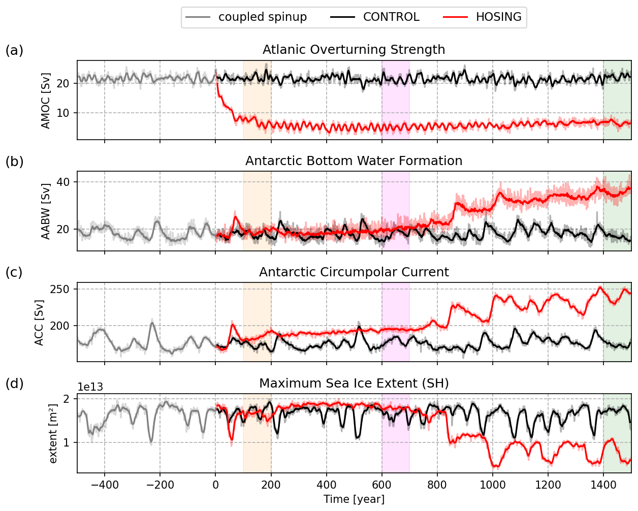
Figure 1 Time series of ocean diagnostics: (a) AMOC strength in Sv, (b) AABW formation in Sv, (c) ACC strength in Sv and (d) maximum sea-ice extent in the Southern Ocean in m². CONTROL and HOSING simulations are shown in black and red, respectively, and gray lines show the end of the spinup. The start time of HOSING is set to year 0. Solid lines show 10 year running mean of the yearly (lighter coloured) data. The three shaded areas show the 100 year time periods that are discussed further in Sect. 3.2–3.4.

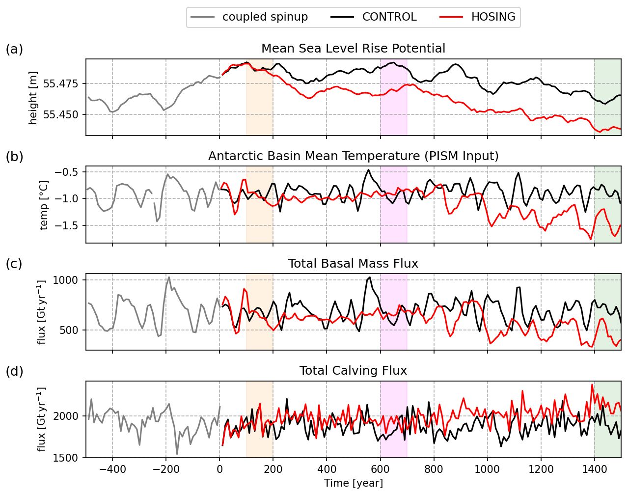
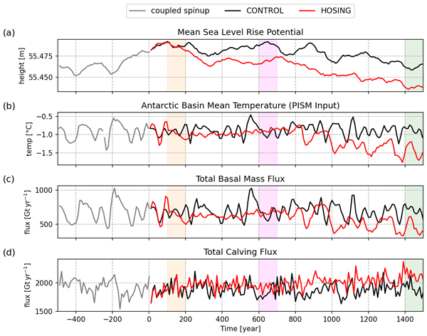
Figure 2 Antarctic Ice Sheet time series: (a) Sea-level-rise potential in m, (b) oceanic temperature forcing (averaged for ocean depths between 500–1000 m) in °C as the Antarctic basin mean, (c) total basal mass flux in Gt yr⁻¹ and (d) total calving flux in Gt yr⁻¹. The CONTROL and HOSING simulations are shown in black and red, respectively, and gray lines show the end of the spinup. The start time of HOSING is set to year 0. All data are presented with a decadal temporal resolution. The three shaded areas show the 100 year time periods that are discussed further in Sects. 3.2–3.4.

Figure 2 shows the transient response of the AIS to an AMOC collapse. The total change in the ice sheet volume is comparably small, as it barely exceeds the range of internal variability during the coupled spinup. Sea-level-rise potential (SLRP) with respect to the CONTROL experiment is decreased by around 2.5 cm after 1500 years (Fig. 2a), without showing any abrupt deviations during the whole integration. Because PISM is only exposed to oceanic changes in our configuration, the main drivers of change in the ice sheet are basal melting and calving fluxes. Both fluxes are subject to oceanic temperature and salinity anomalies, which the model extracts from ocean depths between 500 and 1000 m, depending on the glacial basin. Basal mass and calving fluxes in HOSING are within the range of variability of CONTROL in the first 800 years of the simulation (Fig. 2c and d), because during this period mean subsurface ocean temperature forcing in HOSING is in the range of values in CONTROL ($-\mathrm{0.85}\pm \mathrm{0.4}\mathrm{°}\mathrm{C}$) (Fig. 2b). There is less variability in the ocean temperature, explaining the decrease of basal mass variability (Fig. 2b and c). Calving, on average, is 3 % larger than in CONTROL, driving the slight decrease in Antarctic mass (Fig. 2a and d). With the shift of AABW formation at around 830 years, the average ocean temperature across all basins decreases to −1.5 °C in HOSING (Fig. 2b). This drives a subsequent decrease in basal mass flux (mean decrease rate of 160 Gt yr⁻¹) (Fig. 2c). In the same period, an increase in calving flux (on average 170 Gt yr⁻¹) (Fig. 2d) balances the basal mass decline, leading to similar rates of SLRP changes in HOSING and CONTROL. The reduction in basal melting leads to growing ice shelves that calve more frequently, which explains the increase in calving fluxes. The average ocean salinity across all basins shows a constant negative (freshening) trend (Fig. A14b). This constant decrease of salinity reflects the global freshening due to artificial freshwater forcing, and leads to subsurface conditions supporting basal melt reduction, though the linear trend of decreasing salinity is not reflected in the basal mass fluxes. Antarctic ice mass changes (Fig. 2a) are relatively small in response to the strongly reduced AMOC strength. Overall, in our simulations there is no destabilizing effect of an AMOC shutdown on the WAIS or other parts of the AIS, as hypothesized based on the SO surface warming after an AMOC collapse.

To explain this result, the following sections investigate SO conditions during the HOSING simulation, providing insights into the changes in SO subsurface temperature. We analyse the mean climate states of three time intervals indicated in Figs. 1 and 2. The first period (mean of model years 100–200) is chosen to focus on the time interval that previous studies have investigated (Diamond et al., 2025; Pedro et al., 2018). The second period (mean of years 600–700) represents the climate state before a reduction in maximum Southern Hemisphere (SH) sea ice extent (Fig. 1d) and the onset of deep convection in the Ross Sea. The last time period (mean of years 1400–1500) shows the climate state at the end of our simulation. The climate state of each time period is discussed in the following Sections with a focus on the changes in the SO and adjoint Antarctic ice sheet basins.

3.2 Drivers of shorter-term changes in Southern Ocean conditions (years 100–200)

In the first period, the SO is characterized by positive sea-surface temperature (SST) anomalies up to 1.5 °C south of 50° S (Fig. 3a). This warming, which is robust on the eastern side of the Antarctic continent (see stippling in Fig. 3a), leads to a decrease in maximum sea ice extent and decreasing sea-ice thickness by 5–10 cm in all coastal regions around Antarctica (Figs. 1d and A8a). Sea-ice melt dominates the change in total surface freshwater flux over changes in the precipitation-minus-evaporation balance (Fig. A8d and g) which can regionally decrease surface density. This is outweighed, however, by positive sea-surface salinity (SSS) anomalies originating in the South Atlantic (Fig. 3b), in line with results shown by Zhu and Liu (2020), which diffuse across the ACC leading to a net increase in surface density in much of the SO (Fig. 3c), particularly the Weddell Sea region. In CONTROL, the Weddell Sea is the only SO region where convection occurs (similar results of Zhang et al., 2019). This vertical mixing changes little in HOSING (Fig. 3e), shifting southwards due to reduced sea ice and more negative wind stress curl (Figs. 3f and A4d).

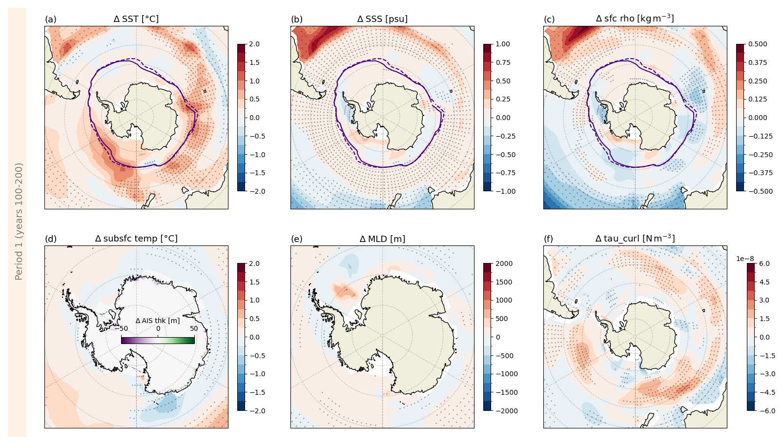
Figure 3 Southern Ocean anomalies of (a) sea surface temperature in °C, (b) sea surface salinity in psu, (c) sea surface density in kg m⁻³, (d) averaged ocean subsurface temperatures between 500 and 1000 m in °C and land ice thickness on the AIS in m, (e) maximum mixed layer depth in m and (f) wind stress curl in N m⁻³. Each panel shows anomalies with respect to CONTROL as a 100 year average for the first time period indicated in Fig. 1. Purple contours in the top row show the maximum sea-ice extent where concentration is larger than 15 % per grid cell for CONTROL (dashed line) and HOSING (solid line). Overlaid light grey stippling shows regions with significant changes in HOSING (see Sect. 2.2 for test description). Latitude graticules are plotted with a 10° grid spacing.

The atmospheric warming (Fig. A4a) south of 65° S leads, on average, to an ocean warming from the surface down to around 250 m (Fig. A11a–c). However, temperature anomalies are negative in subsurface depths (500–1000 m) in this region (Fig. 3d) between years 100 and 200. This cooling originates in the North Atlantic, as residual North Atlantic Deep Water (NADW) transports the cooling signal of the collapsed AMOC to the SH. The inflowing NADW is upwelled mainly in the Atlantic sector and reaches the waters close to the Antarctic continent approximately in model year 100 (Fig. 4b). The ACC transports this signal along the coast, spreading it to all sectors of the SO (Fig. A11a–c). In regions without convection, we find that the cooling strengthens with time and represents a significant signal in the east of the Antarctic continent (see stippling in Fig. 3d). Inflowing water masses also drive a freshening trend (decrease of 0.1 % per year) in the same subsurface depths (Fig. 4d). These changing subsurface conditions are decisive for the evolution of the AIS.

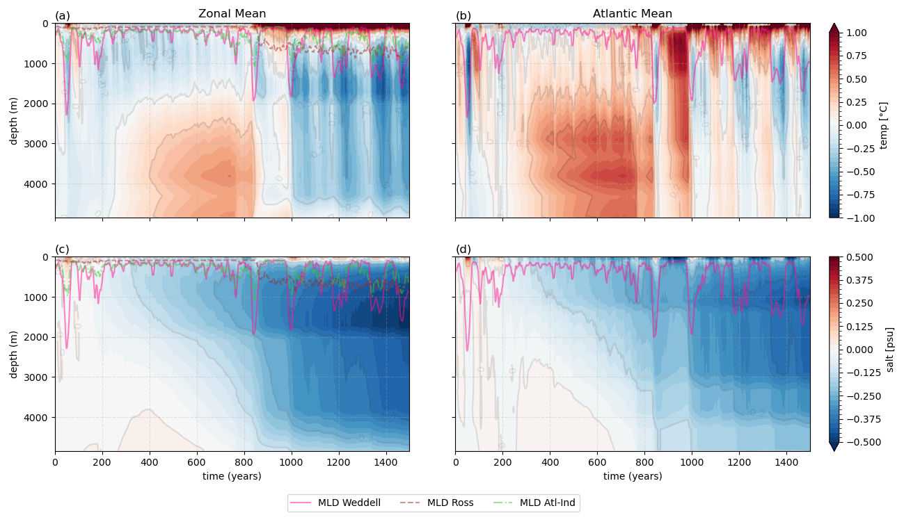
Figure 4 Hovmöller plots of (a, b) temperature in °C and (c, d) salinity anomalies in psu with respect to a 500 year mean of the CONTROL in the Southern Hemisphere, south of 65° S. Subplots (a, c) show averages over all longitudes, (b, d) averages over the Atlantic Sector. Overlaid time series show the maximum mixed layer depth (MLD) averaged over the Weddell Sea ($\text{lon}=\left[\mathrm{60}\text{–}\mathrm{0}\mathit{°}\mathrm{W}\right],\text{lat}<-\mathrm{65}\mathit{°}\mathrm{S}$) (pink line), the Ross Sea ($\text{lon}=\left[\mathrm{150}\mathit{°}\mathrm{E}\text{–}\mathrm{150}\mathit{°}\mathrm{W}\right],\text{lat}<-\mathrm{65}\mathit{°}\mathrm{S}$) (brown, dashed line) and the east of the Weddell Sea (Atl-Ind) ($\text{lon}=\left[\mathrm{0}\text{–}\mathrm{60}\mathit{°}\mathrm{E}\right],\text{lat}<-\mathrm{65}\mathit{°}\mathrm{S}$) (green, dash-dotted line).

The temporal evolution of basal mass flux is strongly aligned with the mean subsurface ocean temperatures (between 500 and 1000 m depth), which decrease by around 0.15 °C (Fig. 2b). Therefore, between years 100 and 200, changes of basal mass flux show on average a decrease up to 100 Gt yr⁻¹ after 200 years in HOSING (Fig. 2c). Resulting AIS thickness changes are limited to the coastal regions and mostly smaller than 5 m (Fig. 3d). Despite the decrease of basal melt in most regions, there is a peak of mean basal mass flux in the Atlantic sector around year 90 of our HOSING simulation (Fig. A12, basin 1). It results due to several years with less convection in which subsurface temperature anomalies in the Weddell Sea are positive (maximum positive anomaly of 0.4 °C between year 80 and 130) (Fig. 4b). The reduced vertical mixing, which does not yet represent a regime shift compared to CONTROL (see stippling in Fig. 3e), stops the heat release from subsurface waters to the atmosphere (Fig. A5d), driving a briefly increase of melt rate up to 200 Gt yr⁻¹ that is reflected in decreasing AIS thickness of the Filchner–Ronne ice shelf. These thickness changes dominate the 100 year mean AIS thickness anomaly (Fig. 3d). Local ice-sheet changes are therefore directly linked to the changing frequency of convection in the Weddell Sea, which impacts interior temperature and salinity changes of coastal ocean waters. Similar fluctuations also exist in the spinup and CONTROL, which explains why results in this period are mostly not significant in the Weddell Sea region (see stippling in Fig. 3).

3.3 Reduced Southern Ocean convection leading to subsurface heat accumulation (years 600–700)

The intermediate part of our simulation (years 600–700) is analysed to present ocean and SH climate conditions before the climatic shift, ie. the onset of deep convection in the SO. In this period, SSTs in most regions south of 60° S other than over Prydz Bay in East Antarctica show negative anomalies (Fig. 5a). This is caused by an increase in sea ice, as after approximately 250 model years, sea ice in the SH regrows and its maximum extent exceeds that of the CONTROL run (see contour lines in Fig. 5a–c). Sea-ice thickness increases in the Weddell and Ross Sea region (Fig. A8b) by 5–20 cm and variability of the averaged maximum sea-ice extent decreases compared to CONTROL (Fig. 1d). Thereby less deep warm water is upwelled and sea surface temperatures as well as surface–air temperatures over and close to Antarctica show a cooling signal (Figs. 5a and A4b). The maximum cooling in this time period is −3 °C over parts of the Weddell Sea and over the Amundsen and the Ross Sea. The wind stress curl at the ocean surface intensifies along the maximum sea-ice edge, especially in the Bellingshausen and Amundsen Sea (Fig. 5f). Thereby, fresher circumpolar deep water is upwelled, conveying the low salinity signal of the North Atlantic hosing (Figs. 4c, d, and A9e). We therefore see negative SSS anomalies (Fig. 5b), despite less freshwater flux due to sea-ice melt south of 70° S (Fig. A8e), and surface densities south of 60° S decrease on average by 0.25 kg m⁻³ (Fig. 5c) in all sectors except for the eastern part of the Pacific sector and latitudes north of 70° S in the Pacific. Positive sea-surface salinity anomalies (up to +0.5 psu) in the eastern Bellingshausen Sea (Fig. 5b) are probably transported there from the South Atlantic, as the Ross Sea gyre is strengthened over time (Fig. A7e) and increases the water transport from the ACC towards the margin of the Antarctic continent (Wang et al., 2024).

Decreased densities of upwelled waters increase surface stratification, leading to a strong decrease in vertical mixing (maximum mixed layer depth (MLD) reduction of around 1250 m) in the Weddell Sea (Fig. 5e). Therefore, variability of AABW formation (Fig. 1b) decreases in this time period. The reduced convection drives an increase of subsurface temperatures in the Atlantic sector by a maximum of 0.5 °C at depths of 500–1000 m (Fig. 5d), as sensible and latent heat loss to the atmosphere is reduced (Fig. A5e). As a result, basal mass fluxes slightly increase in this region compared to CONTROL (Fig. A12, basin 1), however AIS thickness anomalies have the same magnitude as in the previous time period (see Sect. 3.2), i.e. ice loss does not accelerate (Fig. 3d). With the reduction in Weddell Sea convection, heat begins accumulating in the deep SO below 2000 m in all ocean basins (Figs. 4a, b, and A10a, b). Salinity values below 2000 m show increasing negative anomalies, which originate from subsurface depths and over time diffuse to the deep SO (Figs. 4c and A9e).

In all other ocean sectors, the density of intermediate waters continue to decrease, driven by the freshening of upwelled NADW in the SO that is transported around the Antarctic continent by the ACC, as discussed for the previous time period in Sect. 3.2. Therefore, in the Indian and Pacific sector we find negative subsurface temperature anomalies (up to −1 °C) along the coast (Fig. 5d), as well as decreasing salinity in subsurface depths in all regions south of 50° S, up to −0.45 psu (Fig. A3e). These changes in subsurface ocean forcing (temperature and salinity) between years 200 and 800 therefore show the continuation of the trends seen in the previous time period. Consequently, the response of the AIS is very similar, showing an averaged change of basal mass flux decrease of 100 Gt yr⁻¹ with respect to CONTROL (Fig. 2c) and an increase in calving flux of the same rate (Fig. 2d). Both signals are most evident in ice-sheet basins in the Ross Sea region as well as basins close to and east of the Amery ice shelf (Fig. A12), where AIS thickness anomalies are also positive (Fig. 5d).

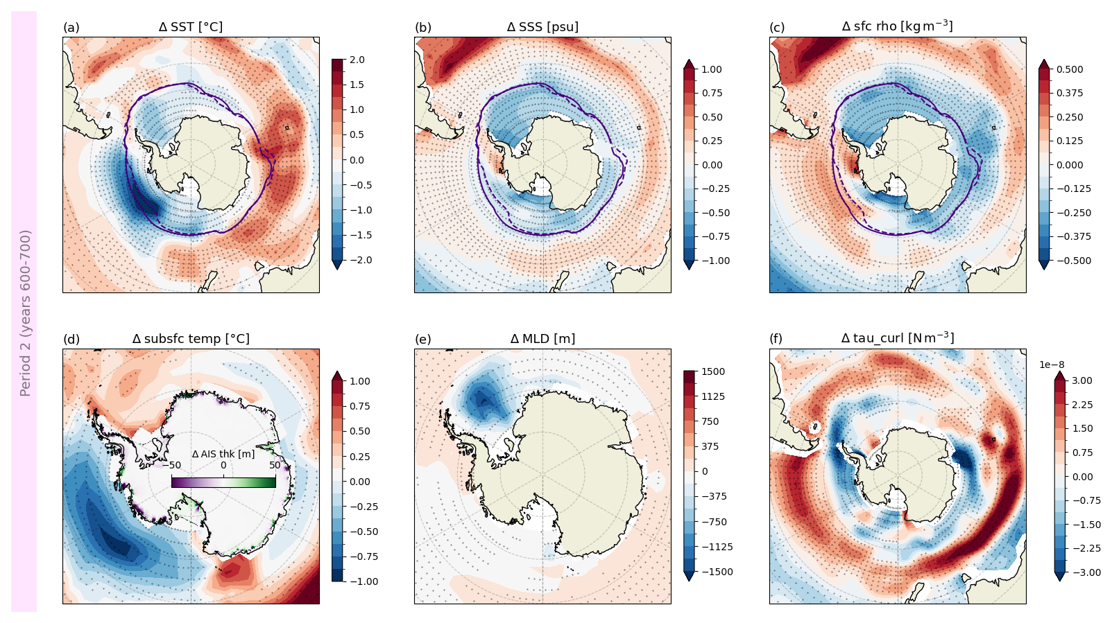
Figure 5 Southern ocean anomalies of (a) sea surface temperature in °C, (b) sea surface salinity in psu, (c) sea surface density in kg m⁻³, (d) averaged ocean subsurface temperatures between 500 and 1000 m in °C and land ice thickness on the AIS in m, (e) maximum mixed layer depth in m and (f) wind stress curl in N m⁻³. Each panel shows anomalies with respect to CONTROL as a 100 year average for the second time range indicated in Fig. 1. Purple contours in the top row show the maximum sea ice extent where concentration is larger than 15 % per grid cell for CONTROL (dashed line) and HOSING (solid line). Overlaid light grey stippling shows regions with significant changes in HOSING (see Sect. 2.2 for test description). Latitude graticules are plotted with a 10° grid spacing.

3.4 Southern Ocean heat release by increased convection (years 1400–1500)

From year 700 onwards, vertical mixing in the Weddell Sea progressively increases, down to 2000 m depth (Fig. 4a). Convection in the Ross Sea starts to ventilate the deep SO (Fig. 6e) from year 830 onwards, mixing water columns in this region continuously every year (Fig. 4b). Convection starts due to the growing water column instability driven by the accumulation of heat in the deep SO in previous centuries (Fig. 4a) as well as decreased salinity of subsurface waters (Fig. 4c). As a result, AABW formation in HOSING increases by 15 Sv with respect to CONTROL at the end of the simulation (Fig. 1b), exhibiting an anti-phased behaviour of NADW and AABW formation (Barbante et al., 2006; Peltier and Vettoretti, 2014; Skinner et al., 2020; Willeit et al., 2025). Another contributor to the destabilisation of the SO water column might be changes in temperature of NADW, which is upwelled in the SO (Fig. A9b). As in the study by Pedro et al. (2018), heat accumulates in the South Atlantic, where over time it gradually diffuses to the deep ocean (see Video S1 in the Supplement). This diffusion is a continuous process during the whole simulation, warming over time the NADW that flows to the SH. Consequently, the negative subsurface temperature anomalies in the SO diminish over time and switch to positive anomalies (see Video S1). Around one century after the convection onset in the Ross Sea, water columns also reach instability in other SO sectors, inducing convection in coastal regions eastward from the Weddell Sea to around 70° E (the ocean in front of the Amery Ice Shelf) (Fig. 6e).

Along with the strengthening of convection in the SO there is a resulting increase of global mean SST (Fig. A14a) driven by the release of subsurface heat (Figs. A5f and 6e). The SST increase around the Antarctic continent is around 4 times higher in the climate state after enhanced AABW onset (Fig. 6a) than after the atmospheric warming due to the AMOC collapse (Fig. 3a). In line with this warming, there is a shift in SO sea-ice extent, decreasing to around 55 % of the extent in CONTROL (Fig. 1d). Sea ice is thinning in all regions around Antarctica by up to 50 cm (Fig. A4f).

Furthermore, the increase of deep convection leads to a cooling of Antarctic Bottom waters as heat is released to the surface. This temperature decrease affects all depths, except for the surface layer above ≈500 m (Fig. 4a) and the maximum cooling averaged along the continental slope of Antarctica up to ≈65° S is 1 °C with respect to CONTROL. Due to the climate regime shift in the SO in the last time period the Ross Sea gyre shifts its location again, so that with respect to CONTROL it expands to the east Indian sector in front of Wilkes Land (Fig. A7f). Thereby, cool water masses are transported westward from the Ross Sea and consequently, subsurface temperatures in the East Antarctic also decrease by up to 2 °C (Fig. 6d). In the adjacent ice-sheet basins, the basal mass flux reduces to values close to zero. Especially in the East Antarctic, the calving rates increase by up to 100 Gt yr⁻¹ compared to CONTROL as ice shelves grow larger with less basal melt. In the Weddell Sea subsurface temperatures partly increase along the coast (Fig. 6d), which can be explained by shallower mixed layer depth in the eastern Weddell Sea (Fig. 6e). Reduced heat loss to the atmosphere (Fig. A5f) leads to less pronounced SST warming compared to most other regions around Antarctica (Fig. 6a) and temperature anomalies at 500–1000 m depth are positive (0.05–0.3 °C) along the coastal margin (Fig. 6d). In basins located nearby the Weddell Sea, basal melt increases in years of positive temperature forcing, i.e. only for certain years when no convection site opens up. Basins with ice shelves in Bellingshausen Sea show no significant change in basal mass or calving fluxes (Figs. A12 and A13).

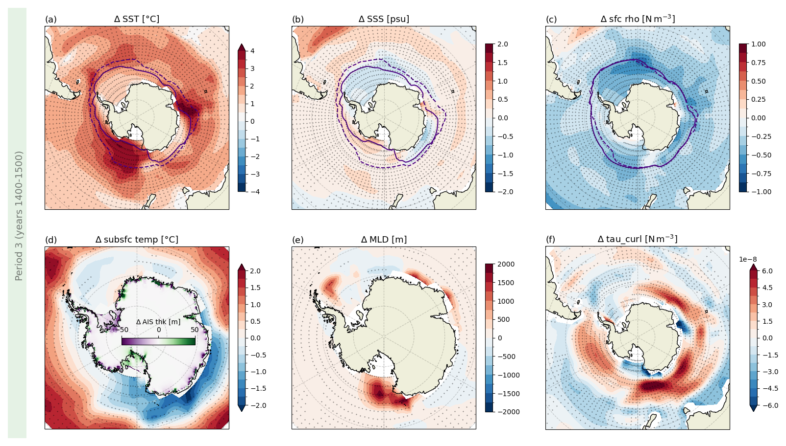
Figure 6 Southern ocean anomalies of (a) sea surface temperature in °C, (b) sea surface salinity in psu, (c) sea surface density in kg m⁻³, (d) averaged ocean subsurface temperatures between 500 and 1000 m in °C and land ice thickness on the AIS in m, (e) maximum mixed layer depth in m and (f) wind stress curl in N m⁻³. Each panel shows anomalies with respect to CONTROL as a 100 year average for the third time range indicated in Fig. 1. Purple contours in the top row show the maximum sea ice extent where concentration is larger than 15 % per grid cell for CONTROL (dashed line) and HOSING (solid line). Overlaid light grey stippling shows regions with significant changes in HOSING (see Sect. 2.2 for test description). Latitude graticules are plotted with a 10° grid spacing.

4 Discussion

The novelty of our study is to simulate the response of Antarctica to an AMOC collapse in an interactively coupled climate and ice-sheet model. We have extended the results of previous freshwater hosing model studies (e.g., Diamond et al., 2025; Orihuela-Pinto et al., 2022; Stouffer et al., 2006), which are mainly focused on atmospheric feedbacks in the Northern and Southern Hemisphere. To capture multi-centennial responses of the AIS, we integrate the model for 1500 years. Even though we could only run one realisation, the simulation length captures possible regime shifts due to internal variability. Contrary to our hypothesis and previous assumptions (see review by Wunderling et al., 2024), the WAIS stays stable during a period with collapsed AMOC, driven primarily by persistently cold temperatures at the depths of the ice shelf cavities. Climate impacts in the first 200 years after HOSING are in good agreement with previous model studies (Diamond et al., 2025; Jackson et al., 2023), which use state-of-the-art CMIP model configurations. In particular, in the SO we find a shift of convection strength in the Weddell Sea in the first century after the AMOC collapse, which partly increases temperatures in the depth range 500–1000 m, similar to the findings of Yeung et al. (2024) for different (last interglacial) boundary conditions. This warming lasts for around one decade and leads to an increase in basal melting which, however, remains within the range of natural variability in the control simulation (CONTROL) and is confined to the Weddell Sea. Testing the significance of convection changes in HOSING (see Fig. 3e) shows, that only a few cells in the Weddell Sea show a significant change, indicating that the change in this time period might be purely induced by centennial variability (which is often simulated in the Weddell Sea in climate models; Zhang et al., 2019). However, it has to be noted, that the applied significant test is based on 100 year means of the CONTROL run that shows regular multi-decadal convective events. This reference distribution is therefore including a multi-decadal variability component, which makes the test not very reliable in the Weddell region. In other regions, Antarctic ice mass does not change.

The AIS response in HOSING slightly shifts after 830 years, as basal melt decreases due to cooling at the depths of ice-shelf cavity inflow. This cooling is caused by an increase in vertical mixing in the SO, which corresponds to the multi-centennial ocean response to the strong AMOC weakening, showing an increase of AABW formation as suggested by Broecker (1998), Skinner et al. (2020) and Willeit et al. (2025). Different studies propose that the oceanic connections between NADW and AABW strength has a different time-scale than the signal propagation of changes by the atmosphere. For example, Swingedouw et al. (2009) distinguish the bipolar climate seesaw (BCS) from the bipolar ocean seesaw (BOS) in the context of a SO freshwater release experiment or Skinner et al. (2020) find that during the Heinrich Stadial 4 enhanced SO convection resulted due to the ventilation seesaw. To the best of our knowledge, our AMOC collapse study is the first one showing an abrupt increase of AABW strength, possibly because model integration times of previous studies were too short. However, Berdahl et al. (2024) did a hosing experiment for 4000 years using CESM2 and discuss a similar cooling of subsurface temperatures during an AMOC collapse. In their study, they do not analyse how ocean convection sites change in the model nor address changes in AABW formation. They explain the subsurface cooling in their simulation by an increase in wind stresses over the SO. Other studies (Rind et al., 2001; Kageyama et al., 2010) with similar setups also show cooling subsurface temperatures in the SO after maximum 500 years of hosing, yet do not address the possible consequences for the AIS. Output of the NaHosMIP models (see Supplemental Material of Diamond et al., 2025) shows that changes in the SO subsurface on the centennial timescale vary drastically between different models (cooling in CESM2, warming in HadGEM3-GC3.1-LL), emphasising that the location, vertical extent and intensity of open ocean convection in the SO are crucial for changes in subsurface water properties, which have direct impacts on the AIS. Even though it takes many centuries for our model to reach an ocean state with strengthened AABW formation in the SO, we note that the impact of this shift is significantly stronger in the Southern Hemisphere than the one of the BCS, which supports findings of Pedro et al. (2016) and Skinner et al. (2020). However, as our study is the first hosing simulation using a coupled climate–ice-sheet model, our results can be unique to our model and configuration, especially the timing of convection onset. Therefore, it is crucial that others repeat this experiment using coupled models, to be able to draw more general conclusions about the interaction between the AMOC and the AIS.

For a simpler comparison to other model runs, we chose to design the freshwater hosing experiment based on the NaHosMIP protocol (Jackson et al., 2023). However, we do not compensate for the artificial freshwater flux (as described in Sect. 2.2), as there is no option to conserve mass via a fresh water flux over the ocean's entire volume in our model. This leads to a constant decrease of ocean salinity throughout the simulation. In our simulation, we apply a freshwater flux of 0.3 Sv in the Arctic region for 1500 simulation years, summing up to a total water volume of approximately 1.3×10⁶ m³. This amount is around 7 times higher than recent estimates of Greenland freshwater forcing (Wouters and Sasgen, 2022) and leads in our model to a total sea level of ≈38.5 m after the 1500 model years (compare to max. SLE of Greenland: 7.42 m; Morlighem et al., 2017). The continuous hosing is however needed to keep the AMOC shut down. The sea level change in the ocean model translates to 0.26 m sea level height change each coupling time step (one decade), yet the used coupling framework does not apply this sea level forcing to the ice sheet model. Applying freshwater without compensation furthermore might lead to a different timing of the AMOC shutdown and change the propagation of temperature and salinity anomaly signals which result from the AMOC shutdown slightly. Regardless of the global salinity change, our results in the first analysed time interval after the AMOC collapsed show global changes in e.g. SST that are very similar to those of previous studies (Jackson et al., 2023; Diamond et al., 2025; Stouffer et al., 2006; den Toom et al., 2014). To the best of out knowledge, there is no literature comparing differences between hosing setups using volume compensations and hosing setups without compensation. Like all hosing experiments, our setup is highly idealised, which nonetheless is a useful approach to advance our understanding of the impacts of an AMOC shutdown on other components of the Earth system.

Our analysis focuses mainly on the temperature changes at intermediate depths (500–1000 m) of the SO, as the trend of decreasing salinity is not reflected in the AIS basal mass fluxes. This can be explained, in part, by the temperature sensitivity of PICO (Kreuzer et al., 2025). Whereas increasing temperatures directly lead to more basal melt, decreasing salinity can impact ice shelf melting mostly via a shift of the freezing temperature. In PICO, melt rates are estimated depending on the equation of state (Eq. (8) in Reese et al., 2018). From this equation results that a change of 0.5 psu, which is the maximum salinity change (basin mean) in the SO after 1500 years of hosing (Fig. A14b), has the same melt effect as a temperature change of 0.02 °C. Therefore the impact of the salinity decline that results of the artificial forcing on basal melting is minimal and the decrease of global ocean salinity is only a second-order effect compared to temperature changes. However, the decreasing salinity trend is crucial to the changes in AABW formation in HOSING from model year 850 onwards. With the current setup, we cannot distinguish between freshening of circumpolar deep water due to the artificial freshwater hosing or due to less salt mixing into the deep ocean after a collapse of the AMOC. Future work is needed, to understand the water export from the hosing region and its impacts in the SO in more detail.

The main motivation of choosing a comparatively low resolution of our climate model is to allow the relatively long integration time of 1500 years plus spinups, though this inevitably leads to shortcomings in the representation of important processes. As the Antarctic continental shelf is not resolved, AABW in the SO is exclusively formed by open ocean convection rather than the export of dense shelf water. Vertical mixing events result as a consequence of weak stratification in the Weddell Sea and Ross Sea (Galbraith et al., 2011). Similar open ocean convection sites occur in 80 % of CMIP6 models (Heuzé, 2021), and are a common weakness in global climate models running at non-eddy-resolving resolutions. A recent study by Aguiar et al. (2025) also argued that the vertical resolution of the ocean surface cell is crucial to simulate AABW formation correctly. In our model setup, deep ocean convection has a large impact on coastal waters at depths where we extract temperature and salinity values with which to force PICO-PISM. The limited resolution of our ocean model lacks features such as the Antarctic slope current that might otherwise block direct signal propagation. The AIS response after ca. 800 years might be distorted by the open-ocean convection regime change. Furthermore, the representation of transport via mesoscale eddies, which plays an important role in heat transport across the ACC, is simplified by the Gent-McWilliams parameterisation (Gent and McWilliams, 1990). As investigated by Pedro et al. (2018), the timing of heat propagation in the SO is probably slower than in eddy resolving models, which would affect the timing of the changes we observe.

The coupling of climate and ice-sheet model (Kreuzer et al., 2021) is based on the sub-module PICO of PISM, which parameterizes the overturning ocean circulation in ice shelf cavities, depending on temperature and salinity of inflowing water masses. PICO bridges the gap between even simpler basal melt parameterisations and high-resolution cavity-resolving ocean models (Burgard et al., 2022). It does not capture all fine-grained details of horizontal melt patterns, but has been proven to compute realistic bulk melt rates and melt-rate sensitivities, locally and on a circum-Antarctic scale, for historic and future scenarios (Reese et al., 2018, 2023). Using PICO enables the co-evolving simulation of the climate and the AIS on millennial timescales by capturing changes of ice fluxes in dependence on the prevailing ocean forcing, and adding resulting meltwater and heat fluxes at realistic depths back into the ocean model. Hence, the model framework captures the expected feedback of increasing basal melt rates in the ice sheet due to increased subsurface ocean temperatures (Paolo et al., 2015) and vice versa.

The sensitivity of the PISM spinup to changes in ocean properties, which can differ greatly depending on the ice-sheet spinup procedure, is not investigated here. In Garbe et al. (2020), a collapse of the WAIS is discussed as a response to increased ocean temperature forcing. This collapse results from marine ice sheet instabilities in regions with retrograde sloping bedrock, even though it is argued that the setup is not in line with observations (Mouginot et al., 2014; Joughin et al., 2014). Therefore they suggest that especially ice shelves in the Amundsen Sea are more sensitive to an increased ocean forcing than in their study. As our study adopted the spinup state from Garbe et al. (2020), the PISM configuration used here might also be too stable compared to the present-day AIS state.

The model setup used for this study has no coupling between PISM and the AM2 atmosphere. Therefore, external boundary forcing from the atmosphere to the ice sheet (surface air temperature and precipitation) remains constant throughout the simulation period. Given the fact that under pre-industrial and present-day climate conditions most changes in Antarctica are due to interactions at the ice–ocean interface (Rignot et al., 2019), a missing ice-atmosphere coupling might be reasonable. However, in our simulation air temperatures over the ice sheet and shelves increase between 0.5 and 5 °C due to the AMOC collapse (Fig. A4a and c) along with an increase in precipitation (Fig. A4d and f) located mainly in coastal regions of the AIS. Both factors have opposing effects on the AIS stability. Increased precipitation leads to ice-sheet mass gain, whereas higher surface air temperatures accelerate surface melting. An increase of surface melt favours the formation of melt ponds (van Wessem et al., 2023) and the resulting hydrofracturing increases the risk of further ice loss (Lai et al., 2020). Further possible effects in ice-shelf regions are a reduction in buttressing and higher calving fluxes which can destabilise the ice sheet regionally (Noël et al., 2023; Gilbert and Kittel, 2021). As the precipitation rates in the high Antarctic interior are generally low, also small increases in absolute precipitation can lead to sustained ice growth on the long term. Which effects dominate and whether an additional ice-atmosphere coupling would stabilise or destabilise the AIS remains unclear. The used coupling setup also does not account for elevated meltwater input into the Southern Ocean driven by increased surface melting. Although this is the first study to simulate the response to an AMOC shutdown using an interactive AIS, the limited interaction between climate and ice sheet highlights that future work is needed, using a more integrated coupling to see combined impacts of ocean and atmosphere forcing, by including atmospheric interactions with the ice sheet.

Although the model setup used in this study does not capture all processes, in particular at small spatial scales, our analysis is a first step towards understanding the interaction between large-scale changes in ocean circulation and the Antarctic ice sheet. Future work should strive, where computationally feasible, to better resolve the interactions between the ocean and ice sheet and integrate the impact of the atmosphere. Furthermore, we suggest the non-linearity of the system and the complex behaviour of the SO could prevent the assessment of tipping point interactions based on a single variable that describes the response of the surface ocean (Wunderling et al., 2024). Given the limitations of our approach discussed above, more studies are needed running similar experiments with different coupled model setups (as e.g., Smith et al., 2021). Finally, it would be valuable to investigate the interaction between the AMOC and the AIS in a more realistic scenario, e.g. running the experiments under high emission scenarios or using a more realistic freshwater forcing amplitude that mimics Greenland ice-sheet melting.

5 Conclusions

Our study presents a simplified interactively coupled climate–ice sheet model to investigate the impact of an AMOC collapse on AIS fluxes. Simulating a 1500 year freshwater hosing experiment, we find no destabilisation of the AIS via the ice–ocean interface. Due to changes in SO convection, induced by imported circumpolar deep water, subsurface SO anomalies are cooling and freshening, which results in reduced basal melting. This change is balanced by calving fluxes, as larger ice shelves calve more often. Locally, in our model, changes in the subsurface SO are primarily driven by changes in deep convection. Therefore, the Weddell Sea, where convection happens in a control run, is the only region where temporarily positive temperature anomalies increase ice mass loss from the AIS. Our results indicate that warming SST after an AMOC collapse in the SO are not necessarily sufficient to drive AIS changes, yet anomalies of the ocean waters in depth of ice-shelf cavities might be crucial. Although our methodology has some simplifications, it is the first hosing experiment using a climate–ice sheet model to investigate the millennial response of the AIS. Nevertheless, higher resolutions would be valuable to verify our results, as our ocean model does not resolve continental shelves. In particular in the SO, where eddy fluxes and dense shelf water formation on the continental shelf are main drivers of AABW formation under present-day climate conditions, results could strongly depend on model resolution. One of the main caveats of this study is, that the artificial freshwater hosing over several centuries introduces a constant decrease in global ocean salinity, whose influence cannot be estimated directly. It would therefore be valuable if future work compares the presented results to an additional simulation, which includes volume compensation for the hosed freshwater. Additionally, in a scenario of a collapsed AMOC, ice-atmosphere interactions in Antarctica could also become more important than during present-day conditions, leading to increased mass loss or potential instabilities of the AIS. This should be investigated in future studies.

Appendix A: Additional figures HOSING vs. CONTROL

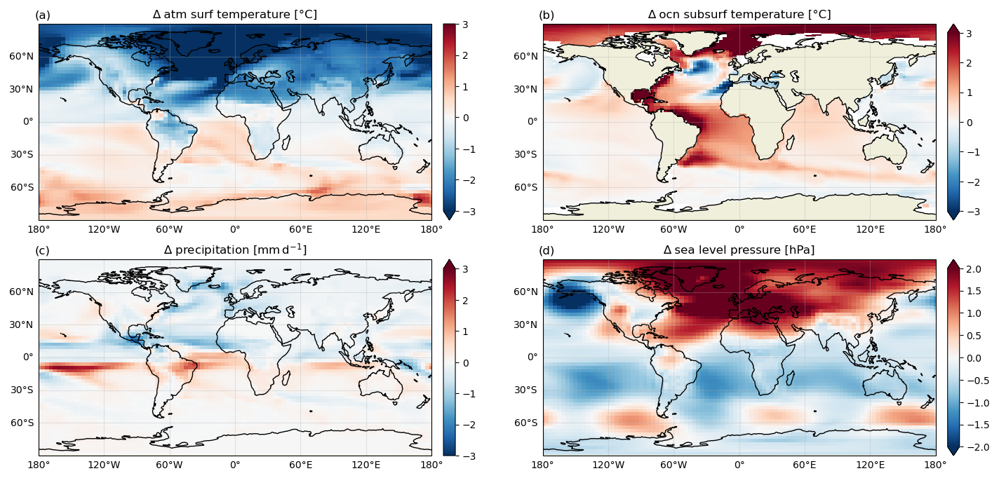
Figure A1 Anomalies of (a) sea surface temperature in °C, (b) subsurface ocean temperature (mean between 500 and 1000 m) in °C, (c) precipitation rate in mm d⁻¹ and (d) sea level pressure in hPa averaged over the first time period (i.e. mean of years 100–200).

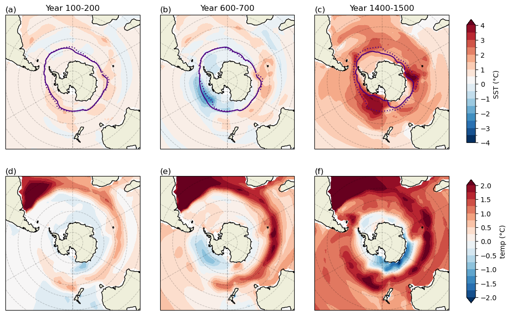
Figure A2 Southern ocean anomalies of (a–c) sea surface temperature in °C and (d–f) averaged subsurface temperatures between 500 and 1000 m in °C. Each column shows a 100 year average for time ranges indicated in Fig. 1. Purple contours in row one show the time averaged maximum sea ice extent where concentration is larger than 15 % per grid cell for CONTROL (dotted line) and HOSING (solid line). Latitude graticules are plotted with a 10° grid spacing. Displayed maps are similar to subplots a and d in Figs. 3, 5 and 6, but shown here in unified colormap ranges for easy comparison.

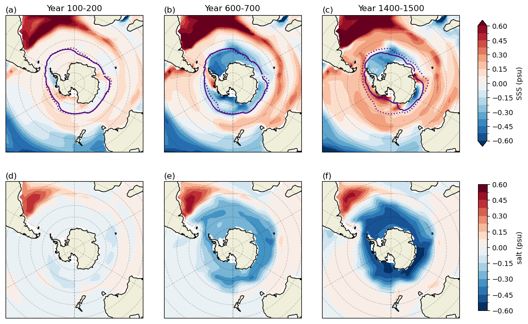
Figure A3 Southern ocean anomalies of (a–c) sea surface salinity in psu and (d–f) averaged subsurface salinities between 500 and 1000 m in psu. Each column shows a 100 year average for time ranges indicated in Fig. 1. Purple contours in row one show the time averaged maximum sea ice extent where concentration is larger than 15 % per grid cell for CONTROL (dotted line) and HOSING (solid line). Latitude graticules are plotted with a 10° grid spacing. Displayed maps are similar to subplots (b) and (e) in Figs. 3, 5 and 6, but shown here in unified colormap ranges for easy comparison.

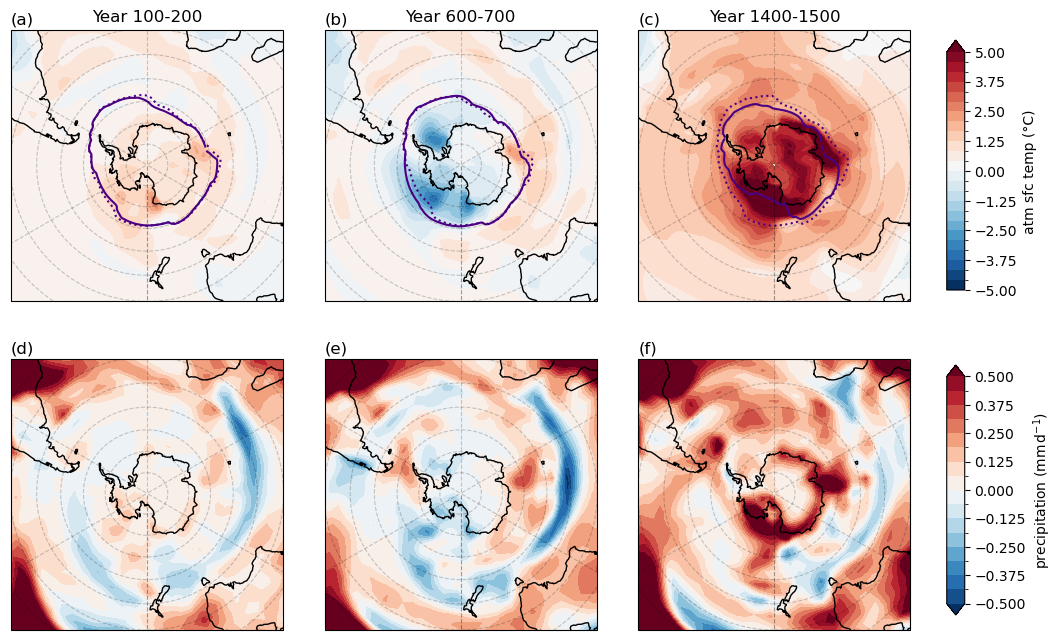
Figure A4 Anomalies of (a–c) atmospheric surface air temperature in °C and (d–f) precipitation (simulated by the atmosphere model) in mm d⁻¹. Each column shows a 100 year average for time ranges indicated in Fig. 1. Purple contours in (a)–(c) show the time averaged maximum sea ice extent where concentration is larger than 15 % per grid cell for CONTROL (dotted line) and HOSING (solid line). Latitude graticules are plotted with a 10° grid spacing.

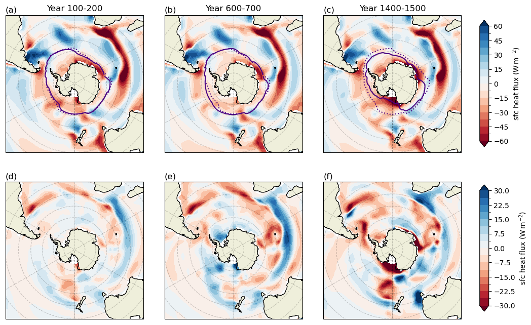
Figure A5 Southern ocean (a–c) HOSING surface heat flux in W m⁻² and (d–f) anomalies of surface heat flux in W m⁻². Each column shows a 100 year average for time ranges indicated in Fig. 1. Purple contours in row one show the time averaged maximum sea ice extent where concentration is larger than 15 % per grid cell for CONTROL (dotted line) and HOSING (solid line). Latitude graticules are plotted with a 10° grid spacing.

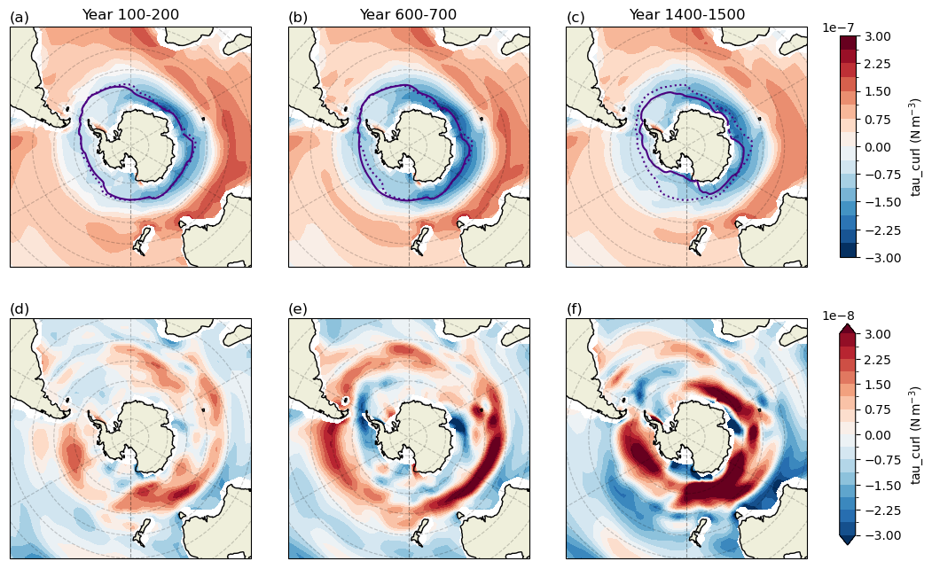
Figure A6 Southern ocean (a–c) HOSING wind stress curl in N m⁻³ and (d–f) anomalies of wind stress curl in N m⁻³. Each column shows a 100 year average for time ranges indicated in Fig. 1. Purple contours in row one show the time averaged maximum sea ice extent where concentration is larger than 15 % per grid cell for CONTROL (dotted line) and HOSING (solid line). Latitude graticules are plotted with a 10° grid spacing. Displayed maps (d–f) are similar to subplots (f) in Figs. 3, 5 and 6, but shown here in unified colormap ranges for easy comparison.

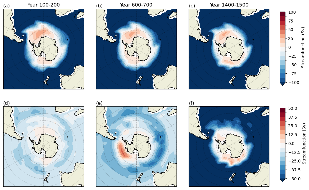
Figure A7 Southern ocean (a–c) HOSING barotropic stream function in Sv and (d–f) anomalies of barotropic stream function in Sv. Each column shows a 100 year average for time ranges indicated in Fig. 1. Purple contours in row one show the time averaged maximum sea ice extent where concentration is larger than 15 % per grid cell for CONTROL (dotted line) and HOSING (solid line). Latitude graticules are plotted with a 10° grid spacing.

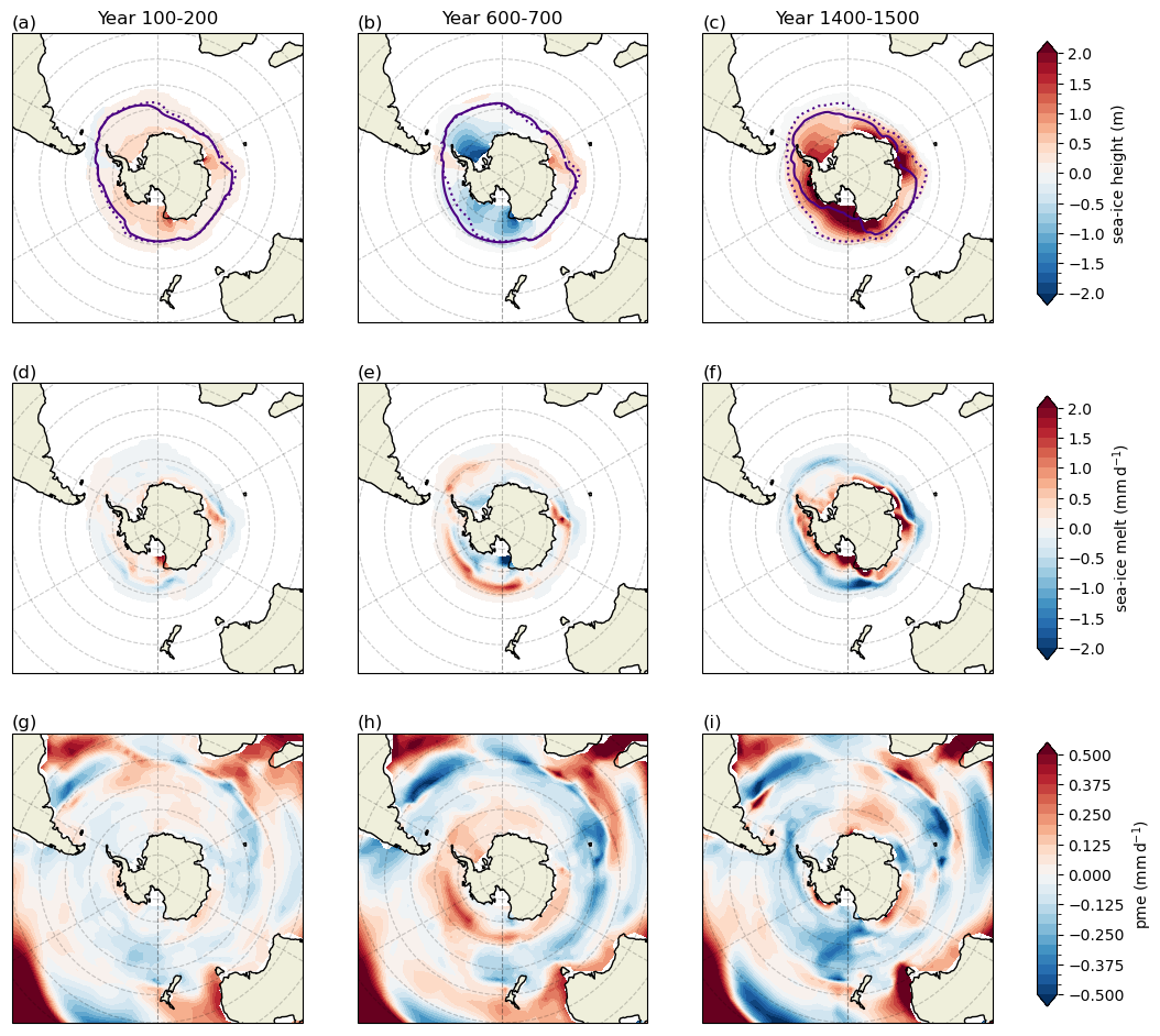
Figure A8 Southern ocean anomalies of (a–c) sea-ice thickness in m, (d–f) sea-ice melt freshwater flux in mm d⁻¹ and (g–i) precipitation – evaporation in mm d⁻¹. Each column shows a 100 year average for time ranges indicated in Fig. 1. Purple contours in row one show the time averaged maximum sea ice extent where concentration is larger than 15 % per grid cell for CONTROL (dotted line) and HOSING (solid line). Latitude graticules are plotted with a 10° grid spacing.

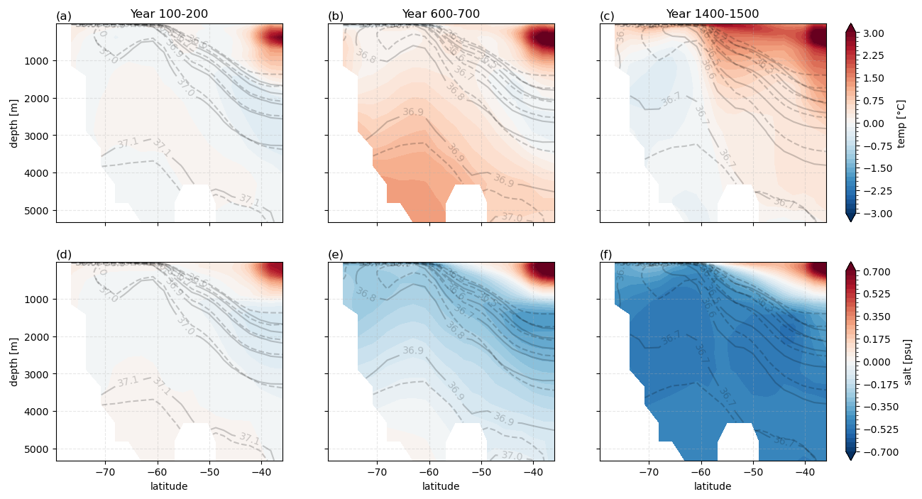
Figure A9 Cross-sections of the Atlantic Sector of the Southern Ocean (south of 35 °S) showing (a–c) temperature anomalies in °C and (d–f) salinity anomalies in psu. Each column shows a 100 year average for time ranges indicated in Fig. 1. Grey contour lines show associated potential densities (referenced to 2000 dbar) in kg m⁻³ for the CONTROL (dashed lines) and HOSING (solid lines) with labels showing the original value of the contour minus 1000 kg m⁻³.

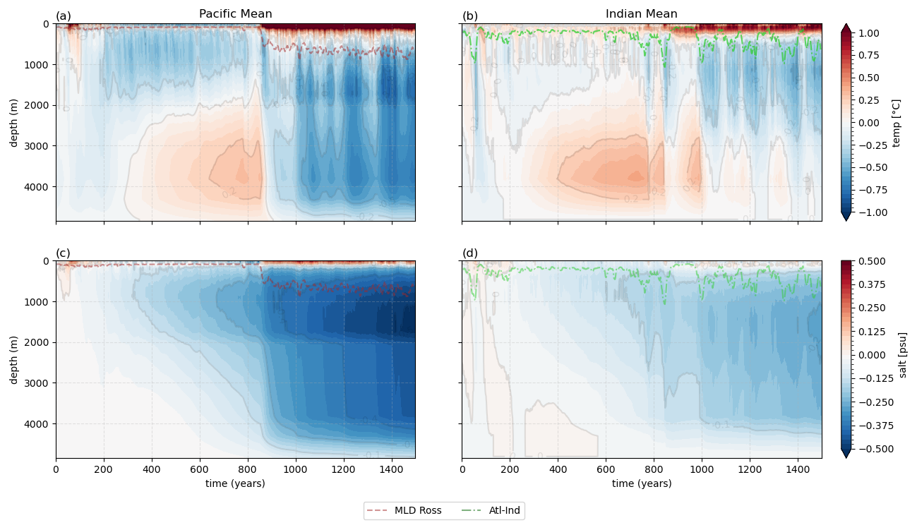
Figure A10 Hovmöller plots of (a), (b) temperature anomalies in °C and (c), (d) salinity anomalies in psu with respect to a 500-year mean of the CONTROL in the southern hemisphere, south of 65° S. (a, c) show averages over the Pacific Sector, (b, d) averages over the Indian Ocean Sector. Overlaid time series show the maximum mixed layer depth (MLD) averaged over the Ross Sea (lon=[150° E–150° W], $\text{lat}<-\mathrm{65}\mathit{°}\mathrm{S}$) (brown, dashed line) and the SO east of the Weddell Sea (Atl-Ind) ($\text{lon}=\left[\mathrm{0}\text{–}\mathrm{60}\mathit{°}\mathrm{E}\right],\text{lat}<-\mathrm{65}\mathit{°}\mathrm{S}$) (green, dash-dotted line).

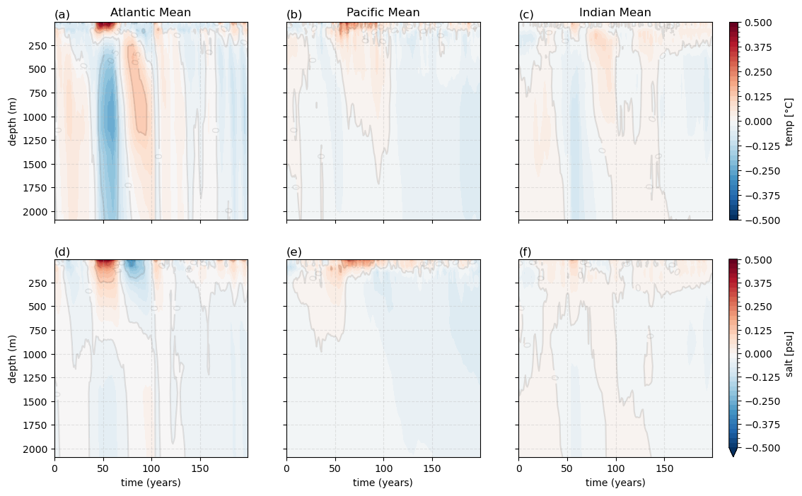
Figure A11 Hovmöller plots of (a–c) temperature anomalies in °C and (d–f) salinity anomalies in psu with respect to a 500-year mean of the CONTROL in the southern hemisphere, south of 65° S. (a, d) show averages over the Atlantic Sector, (b, e) show averages over the Pacific Sector, (c, f) averages over the Indian Ocean Sector. This Figure show the same fields as Figs. 4/A10, but only the first 200 years of the simulation and limited to the upper 2000 m of the ocean.

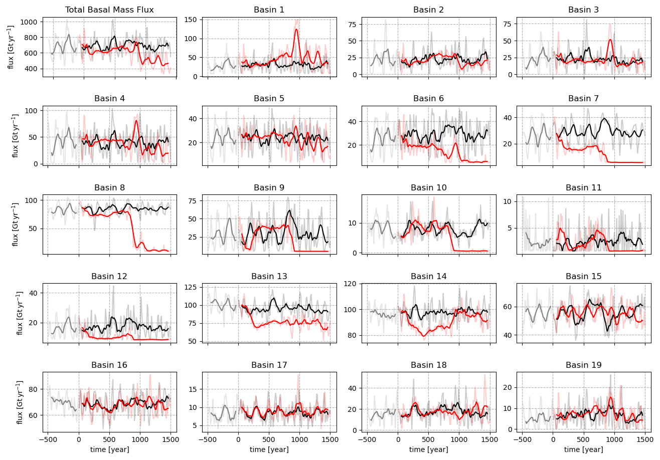
Figure A12 Time series of PISM basal mass fluxes in Gt yr⁻¹ for CONTROL (black line) and HOSING (red line). Upper left panel shows mean of all basins, each of the other panel the series of the basin (defined as in Reese et al. (2018), Fig. 2) specified in the subtitle. Solid lines show 100 year running mean of the decadal (lighter coloured) data.

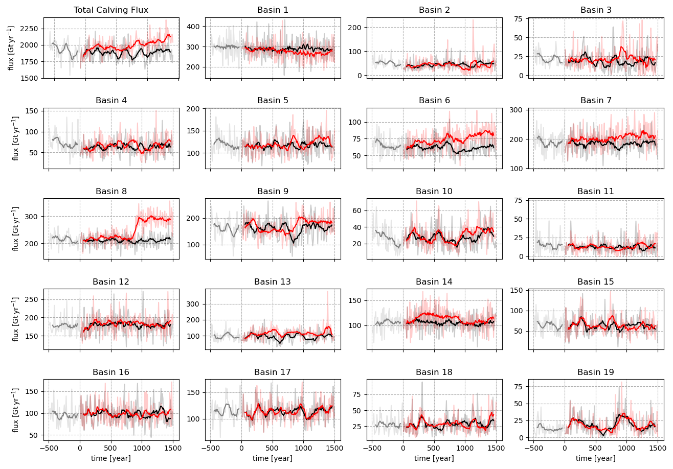
Figure A13 Time series of PISM calving fluxes in Gt yr⁻¹ for CONTROL (black line) and HOSING (red line). Upper left panel shows mean of all basins, each of the other panel the series of the basin (defined as in Reese et al. (2018), Fig. 2) specified in the subtitle. Solid lines show 100 year running mean of the decadal (lighter coloured) data.

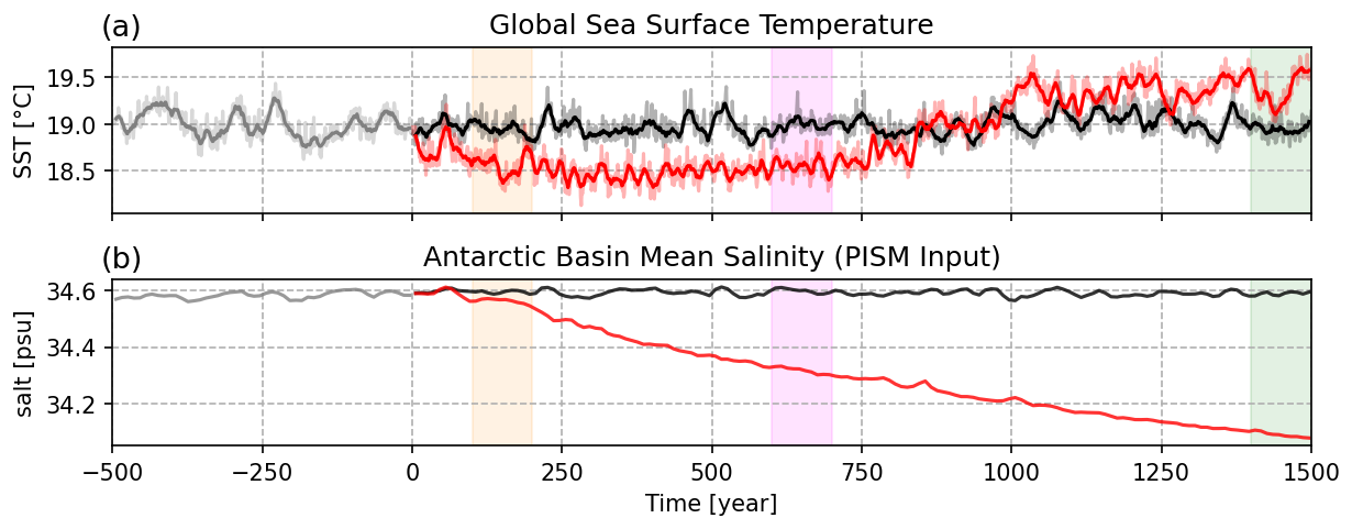
Figure A14 Time series of ocean diagnostics: (a) Global mean sea surface temperature in °C and (b) oceanic salinity forcing in psu as the Antarctic basin mean. The CONTROL and HOSING simulations are shown in black and red, respectively, and gray lines show the end of the spinup. The start time of HOSING is set to year 0. In (a) solid lines show 10 year running mean of the yearly (lighter coloured) data. The three shaded areas show the 100 year time periods that are discussed further in Sect. 3.2–3.4.

Appendix B: Model configuration details

This appendix lists the configuration changes against the example configuration CM2M_coarse_BLING as distributed with the MOM5 code, which we applied in our model configuration.

The changes were inspired by a discussion in the MOM users forum on google groups. That is not public accessible any more, but relevant parts can be found in file exp/CM2M_coarse_BLING/README.CM2M_coarse_
BLING-PIK in our code publication (Kreuzer, 2025a).

• For the atmosphere model, surface topography information was added. It is missing in the example configuration distributed with MOM5.

• Cross-land mixing parameterisation for narrow sea passages between Indonesian islands were taken from Galbraith and de Lavergne (2019).

• To ensure numerical stability with the added freshwater hosing, it was necessary to halve the timesteps for atmosphere, ocean, and coupler exchange between those two.

• To save compute time, the ocean biogechemistry model BLING was switched off.

• The ocean_basal_tracer module was switched on, in order to enable the insertion of basal melt fluxes at depth.

• &ocean_sbc_nml/zero_net_water_coupler=
.false. for the hosing run, in order to disable global correction of artificial freshwater flux.

Some parameters were changed from the MOM5 example configuration towards the original settings as used for the CM2Mc publication (Galbraith et al., 2011), to improve model output with respect to preindustrial conditions.

Appendix C: Additional figures for model spinup evaluation

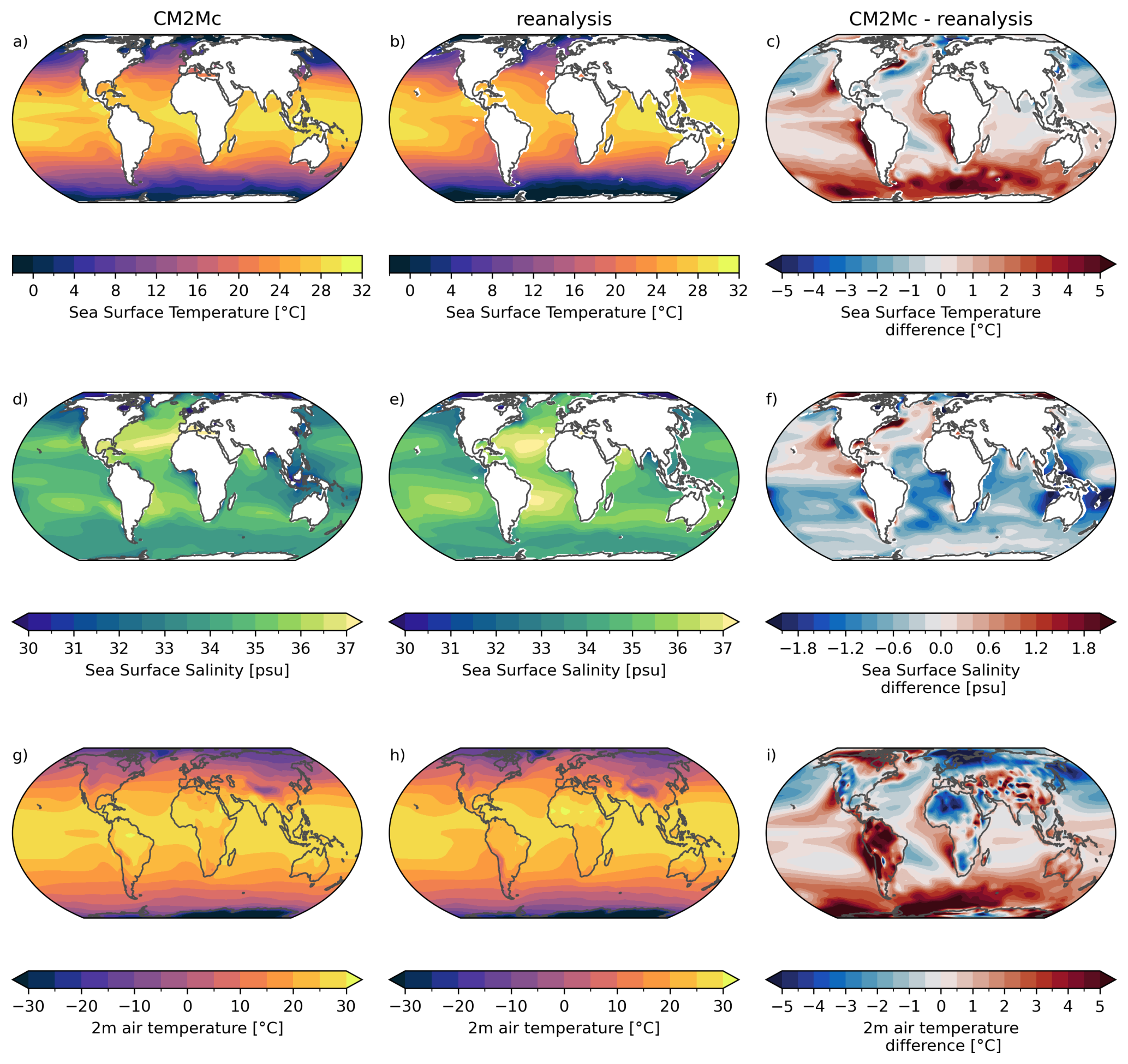
Figure C1 Comparison of CM2Mc–PISM spinup to observations/reanalysis data (surface variables). First column shows sea surface temperature (a), sea surface salinity (d) and 2 m atmospheric air temperature (g) as modeled in the coupled CM2Mc–PISM spinup (100 year mean at the end of the simulation). Second column shows observations/reanalysis data (b, e, h) for comparison. Third column (c, f, i) shows differences between the two. Sea surface temperature and salinity observations are taken from World Ocean Atlas 2018 (time averaged 1955–2017; Locarnini et al., 2018; Zweng et al., 2019). Surface air temperature reanalysis data is taken from ERA-Interim (1979–2013; Dee et al., 2011).

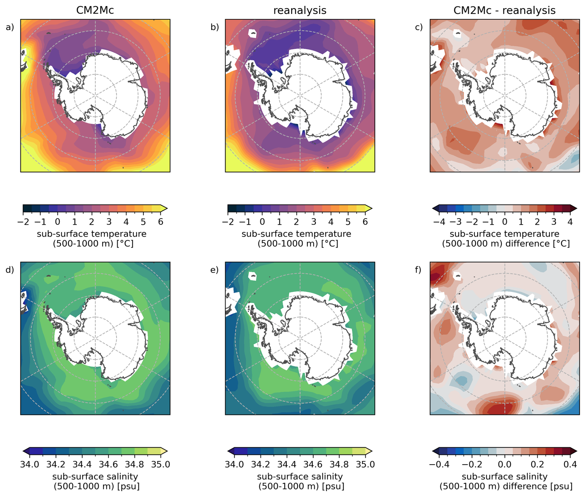
Figure C2 Comparison of CM2Mc–PISM spinup to observations (sub-surface ocean). First column shows ocean temperature (a) and salinity (d) averaged over 500–1000 m depth as modeled in the coupled CM2Mc–PISM spinup (100 year mean at the end of the simulation). Second column (b, e) shows World Ocean Atlas 2018 (time averaged 1955–2017; Locarnini et al., 2018; Zweng et al., 2019) for comparison. Third column (c, f) shows differences between the two.

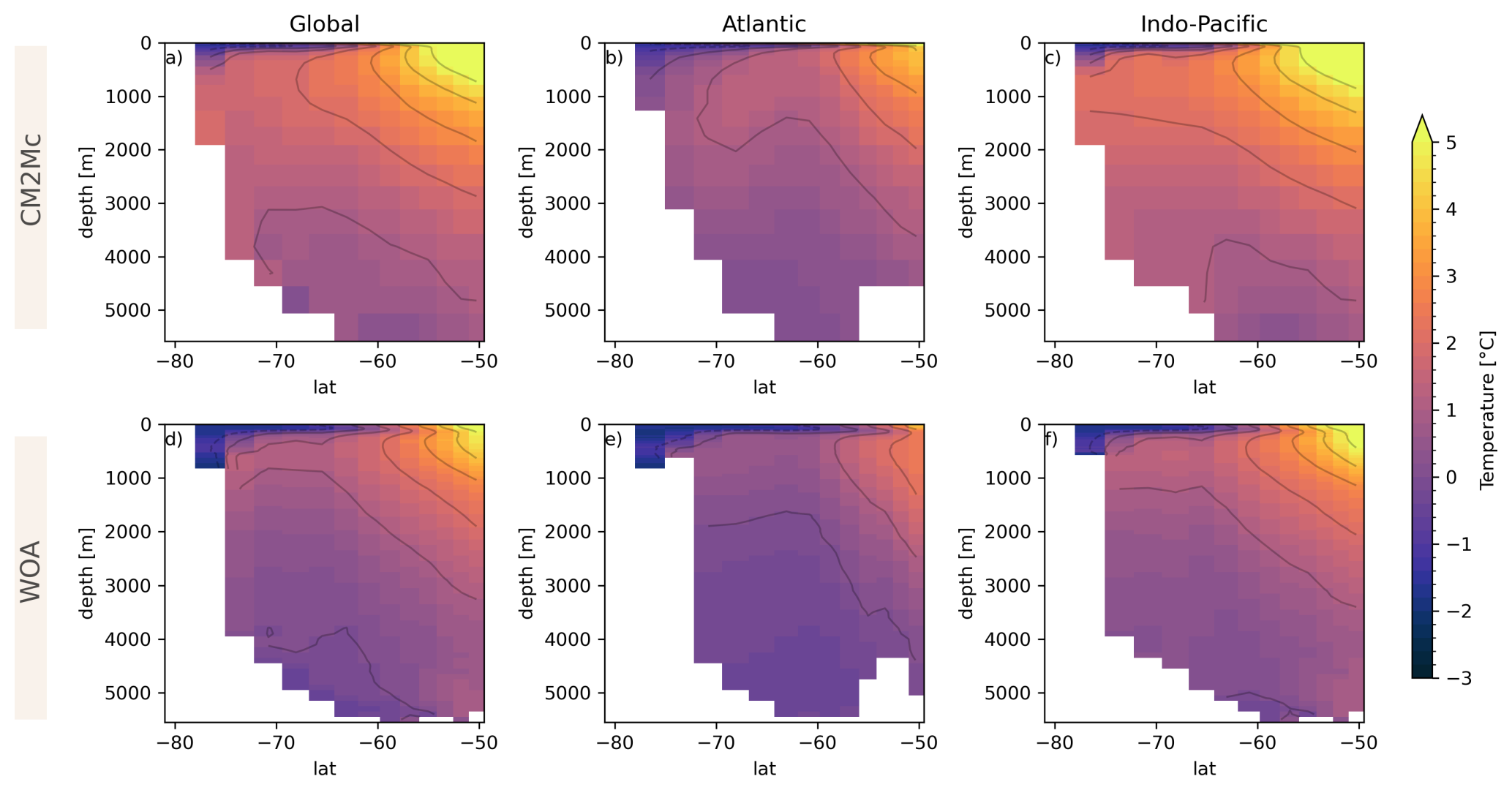
Figure C3 Comparison of CM2Mc–PISM spinup to observations (Southern Ocean temperature cross-sections). First row shows ocean temperatures as Southern Ocean cross-sections averaged over all latitudes (a), over the Atlantic section (b) and over the Indo-Pacific section (c) in the coupled CM2Mc–PISM spinup (100 year mean at the end of the simulation). Second row (d, e, f) shows World Ocean Atlas 2018 (time averaged 1955–2017; Locarnini et al., 2018) for comparison.

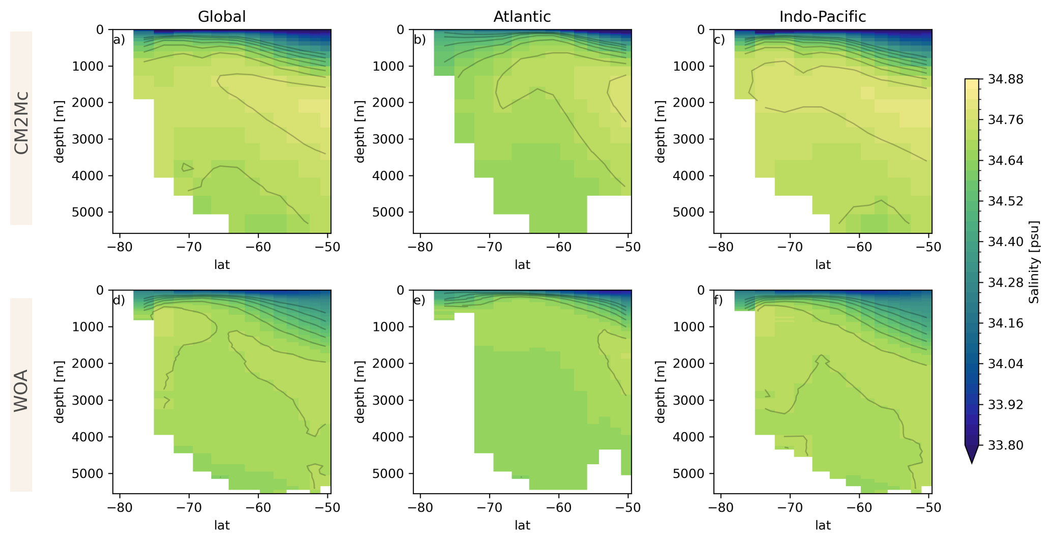
Figure C4 Comparison of CM2Mc–PISM spinup to observations (Southern Ocean salinity cross-sections). First row shows ocean salinities as Southern Ocean cross-sections averaged over all latitudes (a), over the Atlantic section (b) and over the Indo-Pacific section (c) in the coupled CM2Mc–PISM spinup (100 year mean at the end of the simulation). Second row (d, e, f) shows World Ocean Atlas 2018 (time averaged 1955–2017; Zweng et al., 2019) for comparison.

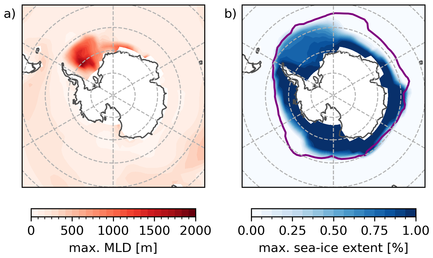
Figure C5 Southern Ocean convection and sea-ice state at the end of the CM2Mc–PISM spinup. The left map shows the mean maximum mixed-layer depth (max. MLD) in m in the Southern Ocean for the last 100 years of the coupled CM2Mc–PISM spinup (a). The right map shows the mean maximum sea-ice extent in the Southern Hemisphere (b) respectively. The purple contour in (b) shows the mean maximum sea-ice extent between year 1979 and 2008, where concentration is larger than 15 % per grid cell, for observational data from the National Snow and Ice Data Center (NSIDC) for comparison (Meier et al., 2021).

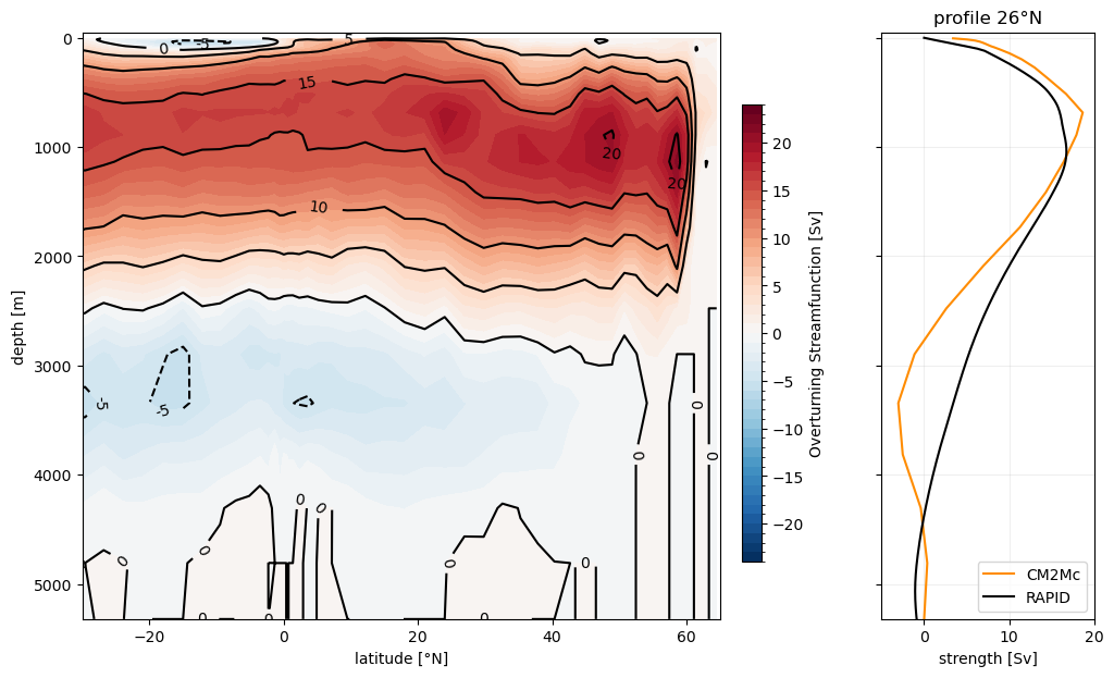
Figure C6 AMOC streamfunction for the CM2Mc–PISM spinup. The left plot shows the Atlantic overturning streamfunction as a mean for the last 100 years of the CM2Mc–PISM spinup. The right plot shows the corresponding AMOC strength profile at 26° N in orange, compared to the RAPID array (Frajka-Williams et al., 2021) profile in black.