Towards robust community assessments of the Earth's climate sensitivity

The eventual planetary warming in response to elevated atmospheric carbon dioxide concentrations is not precisely known. The uncertainty in climate sensitivity (S) primarily results from uncertainties in net physical climate feedback, usually denoted as λ. Multiple lines of evidence can constrain this feedback parameter: proxy-based and model evidence from past equilibrium climates; process-based understanding of the physics underlying changes; and recent observations of temperature change, top-of-the-atmosphere energy imbalance, and ocean heat content. However, despite recent advances in combining these lines of evidence, the estimated range of S remains large. Here, using a Bayesian framework, we discuss three sources of uncertainty – uncertainty in the evidence, structural uncertainty in the model used to interpret this evidence, and differing prior knowledge and/or beliefs – and show how these affect the conclusions we may draw from a single line of evidence. We then propose strategies to combine multiple lines of evidence. We end with three recommendations. First, we suggest that a Bayesian random-effects meta-analysis be used to estimate the evidence and its uncertainty from the published literature. Second, we advocate that the organizers of future assessments clearly specify an interpretive model or a group of candidate models and, in the latter case, use Bayesian model averaging to more heavily weight models that best fit the evidence. Third, we recommend that expert judgment be incorporated via solicitations of priors on model parameters.

1 Introduction

When radiative forcing (ΔF) is applied to the climate system, it induces a radiative imbalance (ΔN) at the top of the atmosphere and a response (ΔR) of the system itself. To first order, ΔR=λΔT, where ΔT is the change in global mean surface temperature. The feedback parameter (λ) thus measures the additional radiative flux density exported to space per unit of temperature change. On sufficiently long timescales, the climate comes into equilibrium (ΔN=0), internal variability is negligible, and we can write a simple energy balance model (denoted M₀) for the climate system. M₀ is expressed as follows:

$$\begin{array}{}\text{(1)}& \mathrm{\Delta }N=\mathrm{\Delta }F+\mathit{\lambda }\mathrm{\Delta }T.\end{array}$$

In the special case where radiative forcing results from a doubling of atmospheric CO₂ relative to its preindustrial concentration of 280 ppm ($\mathrm{\Delta }F=F_{\mathrm{2}\times {\mathrm{CO}}_{\mathrm{2}}})$, the resulting temperature change defines the equilibrium climate sensitivity (S), expressed as

$$\begin{array}{}\text{(2)}& S\equiv -{\displaystyle \frac{F_{\mathrm{2}\times {\mathrm{CO}}_{\mathrm{2}}}}{\mathit{\lambda }}}.\end{array}$$

S is often used as a metric to quantify expected warming in response to radiative forcing but has remained stubbornly uncertain, even as climate models have improved and become more sophisticated. A 2020 community assessment (Sherwood et al., 2020, hereafter referred to as S20) reduced this range using multiple lines of evidence, but the recent Intergovernmental Panel on Climate Change (IPCC) report (Forster, 2021) assessed only “medium confidence” in the upper bound. Is it possible to further narrow the estimated range of S, and can we increase our confidence in this result?

S is determined by the net feedback (λ) at equilibrium and in response to doubled CO₂. While this is unobservable in the current system, in which CO₂ has not yet doubled and is out of equilibrium, several lines of evidence exist that might constrain λ. We have some process-based understanding of individual feedback processes and their correlations, derived from observations and basic physics. We also have evidence from the planet itself, which has been steadily warming in response to net anthropogenic forcing, including emissions of not just CO₂ but also other greenhouse gases and aerosols. Finally, we have proxies that provide evidence about equilibrium climates of the past. S20 attempted to synthesize these three lines of evidence, arriving at constraints on climate sensitivity that narrowed the former range.

In S20, the spread in S arose from reported and assessed uncertainty in historical observations and paleoclimate reconstructions, expert judgment about the uncertainty in physical processes, and the use of different priors on λ and/or S. The IPCC's Sixth Assessment Report (AR6) assessed confidence in the range of S based on support from individual lines of evidence, and the medium confidence assessed was in large part due to the fact that not all lines of evidence supported the same upper bound. By contrast, S20 sought to provide a robust estimate by combining lines of evidence in a coherent Bayesian framework. However, S20 used baseline priors and estimates of the evidence and investigated the impact of alternate choices as sensitivity tests, rather than attempting to combine multiple priors, estimates, and expert judgments into a single posterior probability distribution. In both the IPCC's AR6 and S20, as in almost all previous assessments, the means by which disagreements among experts were resolved or handled were not necessarily made transparent. This paper presents some lessons learned by two authors of S20 and attempts to chart a way forward.

Our goal is to understand where unavoidable subjective decisions enter into the analysis and to present a framework for systematically and fairly incorporating the subjective judgments of multiple experts. Ultimately, we seek to create a framework in which expert judgment is incorporated in the form of clearly specified priors.

The paper is organized as follows. In Sect. 2, we review the basic Bayesian analysis framework. Sections 3, 4, and 5 discuss uncertainty in the evidence, structural uncertainty, and prior uncertainty, respectively. In these sections, we use a single line of evidence – paleoclimate estimates from the Last Glacial Maximum – to illustrate how these sources of uncertainty shape estimates of climate feedbacks and sensitivity. In Sect. 6, we show how these sources of uncertainty affect constraints derived from multiple lines of evidence. In Sect. 7, we propose a new method for combining multiple published studies and multiple models, which may be used in the future to arrive at a robust community assessment of climate sensitivity. Finally, we discuss possible generalizations and extensions.

2 Analysis framework

Bayes' theorem can be written as

$$\begin{array}{}\text{(3)}& P\left(\mathrm{\Theta }\right|Y,M)={\displaystyle \frac{P\left(Y\right|\mathrm{\Theta },M\left)P\right(\mathrm{\Theta }\left|M\right)}{P\left(Y\right|M)}}.\end{array}$$

Here, we will define these terms as they apply to the problem of estimating climate sensitivity.

Evidence.

The evidence (Y) used to constrain climate sensitivity consists of the global mean temperature change (ΔT) in response to forcing (ΔF), as well as, in non-equilibrium states, the net energy imbalance (ΔN). We have estimates of these quantities for the historical period (derived from observations and models) and for past climate states (derived from paleoclimate proxies and models); therefore, Y consists of multiple lines (Y₁…Y_n). For example, S20 used process-based understanding of underlying physics, recent observations, and proxy-based reconstructions of past climates to assess S.

Model.

The model (M) codifies how we interpret the evidence (Y). It specifies the set of parameters (Θ) whose posterior distributions we estimate. For example, in the simple energy balance model, denoted by M₀, there is only one parameter, Θ=λ. The model determines the likelihood $P\left(Y\right|\mathrm{\Theta },M)$ of observing the data given a particular set of parameter values (Θ). We discuss methods for calculating this likelihood in Sect. 3.1.

Prior.

The prior probability distribution P(Θ|M) reflects prior beliefs or knowledge about the set of model parameters (Θ). For example, in the simple model M₀, the S20 community assessment adopted a uniform prior on λ as a baseline choice, choosing not to rule out net positive feedbacks (and, therefore, an unstable climate) a priori. Both the geological evidence and the process understanding presented in Sect. 3 of S20 effectively rule out both positive and extremely negative feedbacks, and thus an alternate prior reflecting this physical knowledge might be a normal distribution, denoted N(μ,σ), with a mean of $\mathit{\mu }=-\mathrm{1.30}$ and a standard deviation of σ=0.44.

This framework allows us to use our prior understanding of the parameter values to calculate the posterior probability $P\left(\mathrm{\Theta }\right|Y,M)$ of the model parameters given the evidence. This posterior can be updated as new evidence becomes available.

Bayesian statistics are both praised and criticized for their inherent subjectivity (see, e.g., Gelman et al., 1995). But all statistical analyses depend on prior knowledge and interpretive models, whether they are implicit or explicit. The Bayesian framework merely makes clear where unavoidable subjective decisions enter the analysis.

Figure 1 Schematic of unavoidable subjective decisions in an analysis of climate feedbacks.

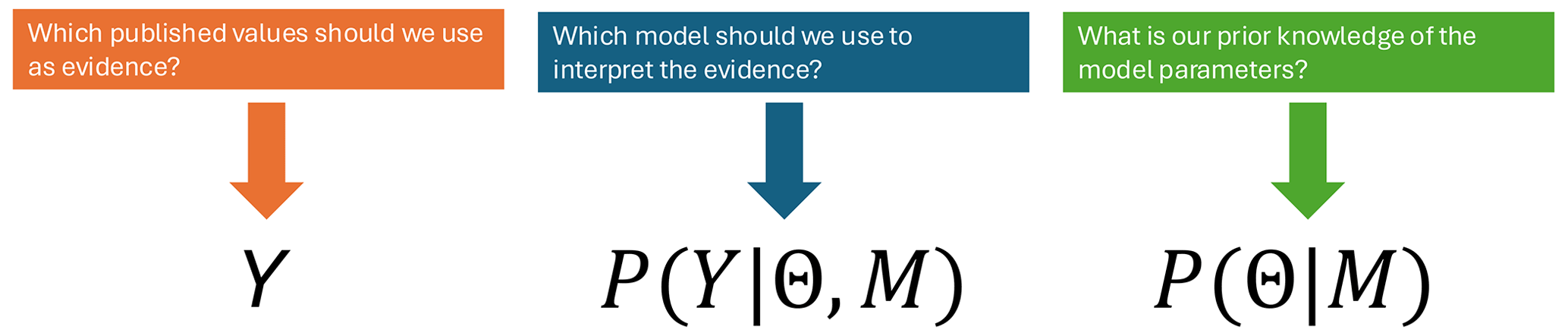
Figure 1 summarizes the decisions that must be made in any Bayesian analysis of climate feedbacks. First, the analyst must decide what constitutes evidence. This requires an assessment of the literature evaluating ΔT, ΔF, and ΔN for each line of evidence. Second, the analyst must specify a model (and its set of parameters, Θ) in order to interpret that evidence. For example, the model M₀ assumes that the feedback parameter is time- and state-independent, and thus estimating the parameter from the past provides a reliable guide to the hypothetical future under doubled CO₂. Finally, the analyst must clearly specify their priors on the model parameters.

In the following sections, we show how different reasonable choices about evidence, models, and priors can lead to very different posterior distributions for λ (and hence for climate sensitivity, S) given a single line of evidence.

3 Evidence uncertainty

The strongest constraints on equilibrium climate sensitivity in S20 were derived from paleoclimate evidence, with the closest equilibrium climate to that of the present being the Last Glacial Maximum (LGM), approximately 21 000 years ago. Reconstructions (Annan and Hargreaves, 2013; Bereiter et al., 2018; Friedrich et al., 2016; Holden et al., 2009; von Deimling et al., 2006; Shakun et al., 2012; Snyder, 2016) or model-based estimates (Braconnot et al., 2012; Kageyama et al., 2021) of the global mean temperature change (ΔT) and radiative forcing (ΔF) have been used to calculate the global mean feedback (λ) inferred from this period. Neither of these observed quantities is precisely known. For example, multiple seemingly incompatible estimates of the LGM global mean cooling (ΔT) are available in the published literature (Annan and Hargreaves, 2013; Holden et al., 2009; Shakun et al., 2012; von Deimling et al., 2006; Friedrich et al., 2016; Hansen et al., 2023; Annan et al., 2022; Bereiter et al., 2018; Snyder, 2016; Kageyama et al., 2021). These estimates are derived from climate models participating in the Paleoclimate Modelling Intercomparison Project (PMIP; Kageyama et al., 2021), as well as from combinations of models and various proxies, and are often in conflict with one another.

We will illustrate the impact of this uncertainty by comparing the evidence used in two recent studies. S20 used expert judgment applied to a literature review to estimate $\mathrm{\Delta }T=-\mathrm{5}$ K, with a 95 % confidence interval of −3.0 to −7.0 K. However, a contemporaneous study using a new temperature reconstruction (Tierney et al., 2020, hereafter referred to as T20) estimated both colder values (with a mean of −6.1 K) and less uncertain values (with a 95 % highest posterior density interval of −6.5 to −5.7 K) for LGM cooling. We note that the two studies are not exactly comparable: S20 represents a community assessment of evidence that took into account a broad range of evidence and uncertainties, whereas T20 was a single study. The temperature estimates in T20 may also be cold biased and overconfident due to the reliance on a prior derived from a single climate model (Annan et al., 2022). However, in order to illustrate evidence uncertainty, we here treat S20 and T20 as different reasonable estimates of ΔT and ΔF over the LGM. We discuss methods for incorporating estimates, such as those from T20, into expert assessments in Sect. 7.1.

The two studies, S20 and T20, also differ in their estimates of the radiative forcing that led to this temperature change. Both agree that it was colder 21 000 years ago because a change in orbital forcing, while negligible with respect to the global mean, led to the development of large, reflective ice sheets in the Northern Hemisphere and lower levels of atmospheric greenhouse gases. The forcings associated with orbital changes (Kageyama et al., 2021) and CO₂ (Siegenthaler et al., 2005) are relatively well constrained; the forcings from other well-mixed greenhouse gases (Loulergue et al., 2008) and ice sheets are less so, but they are still informed by proxy and model evidence. The forcings from dust (Mahowald et al., 2006; Albani and Mahowald, 2019), other aerosols, and vegetation (Köhler et al., 2010) are highly uncertain. While S20 estimated total radiative forcing at the LGM to be N(−8.43, 2) W m⁻², T20 uses a best estimate of −46.8 W m⁻², with a 95 % confidence interval of −9.6 to −5.2 W m⁻².

The contour lines in Fig. 2a show the joint probability distribution ρ(ΔT,ΔF) (assuming uncorrelated errors) as reported by S20 (black) and T20 (red). Rather than comprising exact measurements of the temperature change and radiative forcing, our evidence (Y) consists of estimates of the joint probability density ρ(ΔT,ΔF).

3.1 Calculating the likelihood

The likelihood of observing this probability density for any given value of the feedback parameter (λ) is determined by the model, which dictates the relationship between λ, ΔT, and ΔF. For example, the simple energy balance model M₀ constrains all possible pairs of ΔT and ΔF to lie along a line with a slope of −λ. Intuitively, the value of −λ that maximizes the likelihood is the slope of the line that passes through the greatest probability density. These maximum likelihood estimates are indicated by straight lines in Fig. 2a.

We therefore define the likelihood of ρ(ΔT,ΔF) for any λ value as the probability mass along the curve (C), as described by the energy balance model with a fixed λ value. This definition is written as follows:

$${\displaystyle }P\left(Y\right|\mathit{\lambda })\propto \underset{C}{\int }\mathit{\rho }(\mathrm{\Delta }T,\mathrm{\Delta }F)\mathrm{d}s,$$

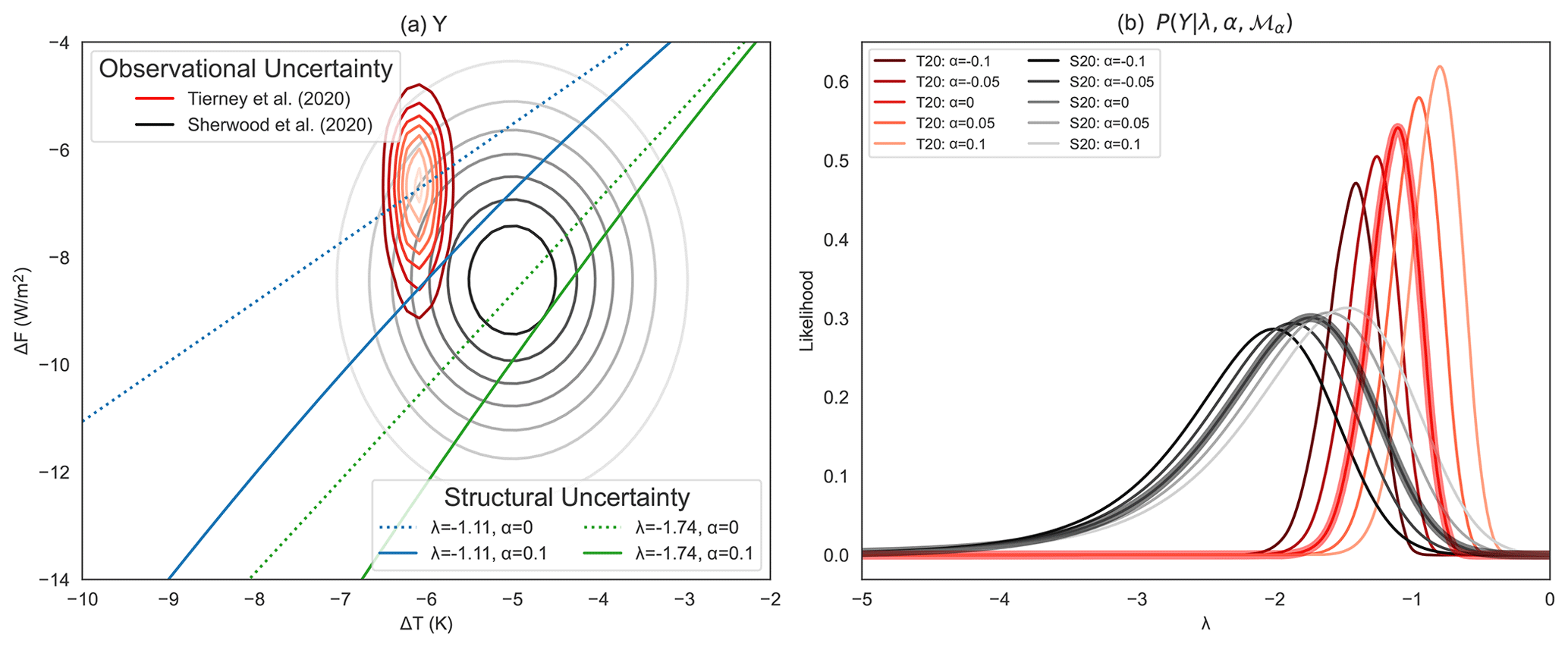
Figure 2 (a) Joint-evidence distributions for ΔT and ΔF used in Sherwood et al. (2020) (black contours) and Tierney et al. (2020) (red contours). Structural uncertainty is illustrated using solid lines (corresponding to fixed values of λ using the model M₀) and dashed lines (corresponding to fixed values of λ and α using the model M_α). (b) Likelihoods as a function of λ given evidence from S20 (black lines) or T20 (red lines) and different values of the state dependence parameter (α). (b) Resulting likelihoods for λ given evidence from S20 (black) or T20 (red) and different values of the state dependence parameter (α). Likelihoods derived using the simple energy balance model (α=0) are highlighted by thick lines.

where C is the curve defined by $\mathrm{\Delta }F+\mathit{\lambda }\mathrm{\Delta }T=\mathrm{0}$. If the joint evidence is a multivariate normal distribution (as it is in S20), this leads to an exact analytic expression for P(Y|λ) (Appendix A). Otherwise, the integral can be computed numerically. The resulting likelihood functions are indicated by thick lines in Fig. 2b.

3.2 Climate sensitivity estimates depend on the evidence

Clearly, the constraints placed on the climate feedback by the Last Glacial Maximum depend on our estimates of the temperature difference and radiative forcing that caused it. Using S20 evidence, this energy balance model, and a uniform prior ($P\left(\mathit{\lambda }\right)=U(-\mathrm{10},\mathrm{10})$), we find that the most likely value of the feedback parameter is $\mathit{\lambda }=-\mathrm{1.7}$ W m⁻² K⁻¹ (thick black line in Fig. 2b), with a 5 %–95 % range of −3.37 to −1.09 W m⁻² K⁻¹. Using T20 evidence, the most likely value is $\mathit{\lambda }=-\mathrm{1.1}$ W m⁻² K⁻¹ (thick red line in Fig. 2b), where the 5 %–95 % range is −1.49 to −0.87 W m⁻² K⁻¹.

For simplicity, here we calculate the likelihood P(Y|λ) and use the resulting posterior, $P\left(\mathit{\lambda }\right|Y)\propto P(Y\left|\mathit{\lambda }\right)P\left(\mathit{\lambda }\right)$, to calculate S (Appendix B). This neglects the small correlation between ΔF and the forcing with doubled CO₂, but this simplification does not substantially affect our results (Appendix C).

Using S20 evidence from the LGM, we find a 5 %–95 % range of 1.17 to 3.69 K for the climate sensitivity (S), assuming, as in S20, that $F_{\mathrm{2}\times {\mathrm{CO}}_{\mathrm{2}}}\sim N(\mathrm{4.0},\mathrm{0.3})$. Using T20 evidence, the 5 %–95 % range for S is 2.61 to 4.72 K.

4 Structural uncertainty

Thus far, we have relied on the simple energy balance model to interpret the LGM evidence. However, many recent studies (e.g., Rohling et al., 2018; Stap et al., 2019; Friedrich et al., 2016; Renoult et al., 2023) have suggested that M₀ might not be appropriate for past climates due to the dependence of the feedbacks on the background climate state. If the relationship between temperature change and radiative forcing is nonlinear, then the feedbacks in a past cold climate should not be treated as identical to those in a future warm climate. To model this background temperature dependence, we might use an alternate model that includes a second-order term in the radiative response. This model (M_α) is given by

$$\begin{array}{}\text{(4)}& \mathrm{0}=\mathrm{\Delta }F+\mathit{\lambda }\mathrm{\Delta }T+{\displaystyle \frac{\mathit{\alpha }}{\mathrm{2}}}\mathrm{\Delta }{T}^{\mathrm{2}},\end{array}$$

where $\mathit{\alpha }=\partial \mathit{\lambda }/\partial \left(\mathrm{\Delta }T\right)$ is an additional parameter reflecting the background state dependence (Sellers, 1969; Caballero and Huber, 2013; Budyko, 1969; Sherwood et al., 2020). Intuitively, nonzero values of α change the relationship between the paleoclimate evidence and the feedback parameter (λ). This, in turn, makes the evidence more or less likely given a value of λ. For example, if $\mathit{\alpha }=+\mathrm{0.1}$ (which translates to a change in feedback of −0.5 W m⁻² K⁻¹ at a cooling of −5 K), the most likely value of λ is not the same as the most likely value of λ when assuming α=0 (dotted and solid lines in Fig. 2a). In this case, the likelihoods (Fig. 2b) are calculated by integrating the joint probability distribution for ΔT and ΔF along the curve defined by Eq. (4), and they depend on the value of the state dependence parameter (α).

If α is not a fixed value but an unknown parameter, then the evidence can constrain only the joint distribution of $\mathrm{\Theta }=(\mathit{\lambda },\mathit{\alpha })$. Obviously, in order for the climate of the past to tell us anything about the climate of the future, we must have some information about how they relate to one another.

There is no limit to the complexity of models we might use to interpret the evidence from the LGM. We might allow for both non-unit forcing efficacy and state dependence. We might assign different efficacies to different forcing agents or allow the parameter α to bifurcate at lower temperatures. We might also include an additive pattern effect (Δλ) that reflects differences in the spatial pattern of temperature change at the LGM and the pattern of warming expected at elevated CO₂ concentrations (e.g., Cooper et al., 2024).

Regardless of the interpretive model used, the model is both required for analysis and subjectively chosen by the analyst. Different reasonable analysts might make different choices about the model that should be used. This means that the choice of model is an important source of uncertainty that must be clearly specified or quantified. There is, however, one more source of uncertainty to discuss. Even with a single model, such as M_α, our degree of confidence in the constraints placed by paleoclimate evidence on the feedback parameter (λ) necessarily reflects our prior knowledge of the state dependence of climate feedbacks. It is to this prior uncertainty that we turn in Sect. 5.

5 Prior uncertainty

Once a model is specified, we aim to use the evidence to gain insights into its set of parameters (Θ). Bayes' theorem states that the posterior distributions of the parameters are simply obtained by multiplying the likelihood by the prior probability distributions, reflecting our preexisting beliefs and/or knowledge. These priors incorporate expert judgment, the results of other analyses, and knowledge of physical processes. Posterior distributions of individual parameters can depend strongly on prior knowledge of all parameters. For example, Fig. 3a shows the joint posteriors for the feedback parameter (λ) and the state dependence parameter (α), assuming the model M_α, the temperature and radiative-forcing values reported in S20, and uniform priors on both parameters.

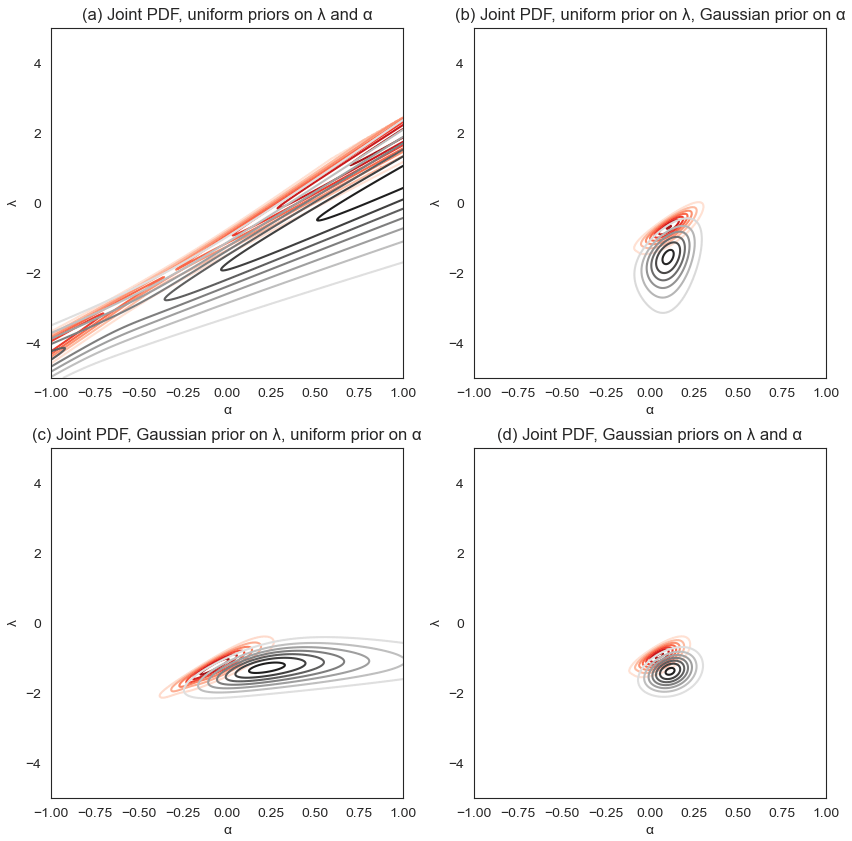
Figure 3 Joint posteriors for the feedback parameter (λ) and the state dependence parameter (α) under the influence of different priors: (a) uniform priors on both parameters; (b) a uniform prior on λ and a Gaussian prior, based on expert judgment from the published literature (used in S20), on α; (c) a Gaussian prior, based on process evidence (used in S20), on λ and a uniform prior on α; (d) and Gaussian priors (from S20) on both parameters. PDF: probability density function.

In the absence of any physical knowledge about these parameters, the joint posterior is not very informative. In fact, considerable posterior weight is placed on extremely large positive values of α and positive values of λ, which would make negative climate sensitivity appear more likely than most scientists would consider credible. A well-informed scientist, however, is unlikely to think that α=1 (which implies an enormous mean change in feedback of −5 W m⁻² K⁻¹ for 5 K of glacial cooling) is just as likely as α=0 (implying no change in feedback). In S20, a prior of $N(+\mathrm{0.1},\mathrm{0.1})$ was assigned to the state dependence parameter (α), reflecting the current state of the literature. This prior substantially constrains the resulting joint posterior distribution (Fig. 3b). Conversely, imposing a more informative prior on the feedback parameter (λ) – for example, by using the process constraints in S20 that result in $\mathit{\lambda }\sim N(-\mathrm{1.30},\mathrm{0.44})$ – also constrains the joint distribution: positive values of α (i.e., values which imply a lower sensitivity at the LGM than for doubled CO₂) receive more posterior weight. Combining the informative priors on both λ and α further constrains the joint posterior (Fig. 3d).

6 Combining multiple lines of evidence

The examples we have presented thus far have all used a single line of evidence – paleoclimate reconstructions of the Last Glacial Maximum – to constrain λ. However, it is not necessary to look back over 20 000 years to gauge the planet's response to external influences. More recently, a large increase in radiative forcing has resulted in significant global warming and a large radiative imbalance at the top of the atmosphere. To constrain λ with transient historical observations, we use the evidence $Y=(\mathrm{\Delta }T,\mathrm{\Delta }F,\mathrm{\Delta }N)$, where ΔN is estimated from observed changes in ocean heat uptake and/or satellite observations constrained by ocean heat content (Forster, 2016).

6.1 Historical likelihood

In this three-dimensional joint probability space, the simple energy balance model M₀ defines a plane, rather than a line, in the evidence space (Fig. 4), and the likelihood of the evidence given λ is proportional to the integral over this surface.

Figure 4 (a) Calculating the likelihood of observing the historical evidence used in S20 for a putative value of λ. Each value of λ defines a plane; shown are $\mathit{\lambda }=-\mathrm{1}$ W m⁻² K⁻¹ (blue), $\mathit{\lambda }=-\mathrm{1.5}$ W m⁻² K⁻¹ (orange), and $\mathit{\lambda }=-\mathrm{2}$ W m⁻² K⁻¹ (green). The likelihood is the surface integral of the joint PDF along the plane. (b) The likelihood of the feedback parameter (λ) given a simple energy balance model with no pattern effect (gray line) and the marginal likelihood of λ given an additive pattern effect with the prior $\mathrm{\Delta }\mathit{\lambda }\sim N(\mathrm{0.5},\mathrm{0.3})$.

Figure 4 shows the historical evidence reported in S20, in which

$$\begin{array}{}\text{(5)}& {\displaystyle }\mathrm{\Delta }T\sim N(\mathrm{1.03},\mathrm{0.085}),\text{(6)}& {\displaystyle }\mathrm{\Delta }N\sim N(\mathrm{0.6},\mathrm{0.18}),\end{array}$$

and ΔF is calculated using unconstrained aerosol effective radiative forcings (ERFs) from Bellouin et al. (2020), with a median of 1.83 W m⁻² and a 5 %–95 % range of −0.03 to 2.71 W m⁻². The gray line in Fig. 4 shows the resulting likelihood as a function of λ. The maximum likelihood value is $\mathit{\lambda }=-\mathrm{1.53}$ W m⁻² K⁻¹.

However, the simple energy balance model M₀ assumes that the feedback parameter is the same for climate changes in the deep past, the transient historical period, and the future. Many studies (e.g., Marvel et al., 2016; Andrews et al., 2018; Dong et al., 2020; Rose et al., 2014; Armour et al., 2013; Gregory and Andrews, 2016; Marvel et al., 2018; Modak and Mauritsen, 2023) now argue that a more appropriate model should include a pattern effect (Δλ) that reflects the differences between feedbacks triggered by the observed spatial pattern of transient warming and feedbacks expected in response to the long-term equilibrium warming pattern. This model (M_Δλ) is given by

$$\mathrm{\Delta }N=(\mathit{\lambda }-\mathrm{\Delta }\mathit{\lambda })\mathrm{\Delta }T+\mathrm{\Delta }F.$$

S20 placed a Gaussian prior on this pattern effect, with $\mathrm{\Delta }\mathit{\lambda }=N(\mathrm{0.5},\mathrm{0.3})$ W m⁻² K⁻¹. This corresponds to a modification of the tilt of the plane shown in Fig. 4a. Because this model assumes that the pattern effect is linearly additive, no further curvature is introduced. By multiplying the joint likelihood ($P(\mathrm{\Delta }Q,\mathrm{\Delta }T,\mathrm{\Delta }F|\mathit{\lambda },\mathrm{\Delta }\mathit{\lambda })$) by the prior (P(Δλ)) and integrating over all values of Δλ, we obtain a marginal likelihood for the historical evidence as a function of the feedback parameter (λ). This is shown by the black line in Fig. 4b. The inclusion of the additive pattern effect and our physics-informed intuition that said effect is likely to be positive shifts the most likely value of the feedback parameter to $\mathit{\lambda }=-\mathrm{1.0}$ W m⁻² K⁻¹.

The pattern effect estimate used in S20 was based on the Atmospheric Model Intercomparison Project II (AMIP-II) dataset, which produces the largest estimate of the pattern effect (Modak and Mauritsen, 2023), and therefore the priors on Δλ used in S20 may be both overconfident and weighted too strongly toward high values. However, while noting this important caveat, for illustrative purposes we will use the S20 historical likelihood marginalized over the pattern effect estimate as the historical likelihood for the rest of this paper.

6.2 The “Twin Peaks” problem

Assuming conditional independence between lines of evidence, the posterior distribution of the feedback parameter (λ) is expressed as

$$\begin{array}{}\text{(7)}& P\left(\mathit{\lambda }\right|Y)\propto P\left(Y_{\mathrm{hist}}|\mathit{\lambda }\right)P\left(Y_{\mathrm{LGM}}|\mathit{\lambda }\right)P(\mathit{\lambda }).\end{array}$$

That is, the posterior estimate of λ given two lines of evidence is proportional to the product of the individual likelihoods. But what if the likelihoods have a small (or no) region of overlap? Can we really be confident that the posterior estimate is well constrained in this case? Figure 5a highlights this potential pitfall. The black line shows the marginal likelihood of the historical evidence as a function of λ. The light-blue line shows the likelihood of the S20 LGM evidence as a function of λ, assuming no state dependence (α=0). The product of these likelihoods is indicated by the dashed green line. The less the historical and paleoclimate likelihoods overlap, the narrower the posterior will be. We refer to this conundrum as the Twin Peaks problem: should greater incompatibility between multiple lines of evidence really reduce the uncertainty in λ? Or could it be that the two lines of evidence are not, in fact, measuring the same thing?

We can take the latter possibility into account using an alternate model for the paleo-evidence. Note that the posterior for λ shown in Fig. 5a is conditional on the model M₀ for the paleoclimate evidence, which contains only one parameter, λ. The model assumes that the equilibrium feedbacks in a warmer climate are exactly the same as those in a colder climate, that the response to pure CO₂ forcing is equivalent to the response to LGM forcings, and that the pattern effect is zero over the LGM. An alternate model, say M_α, allows for state dependence via an additional parameter (α). The marginal likelihood for the paleodata, given M_α and Gaussian priors on α, is indicated by a dark-blue line in Fig. 5b. While the overlap between these two distributions is far from exact, it is substantially larger than that for the no-state-dependence case, illustrated in Fig. 5a. Simply put, the historical evidence and the LGM evidence appear to be more compatible when we correct for the state dependence of the past cold period.

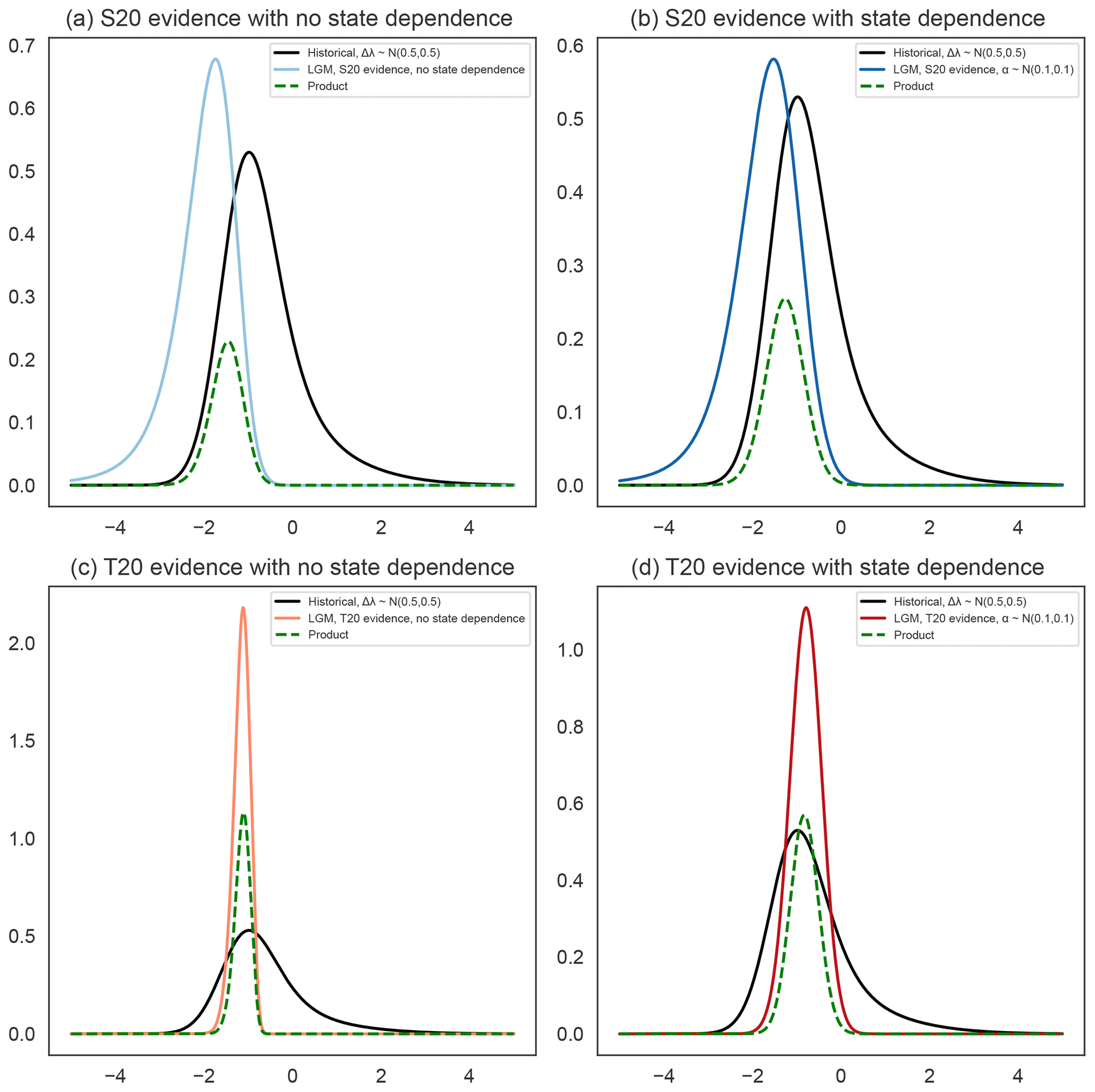
Figure 5 Likelihoods from multiple lines of evidence. In all four panels, the black line shows the likelihood of the historical evidence given λ, assuming the pattern effect $\mathrm{\Delta }\mathit{\lambda }\sim N(\mathrm{0.5},\mathrm{0.3})$. (a) The likelihood of S20 evidence given λ, assuming no state dependence during the LGM (light-blue line) and overlap (dashed green line). (b) The likelihood of S20 evidence given λ, assuming state dependence and $\mathit{\alpha }\sim N(\mathrm{0.1},\mathrm{0.1})$ (dark-blue line), as well as overlap (dashed green line). (c) The likelihood of T20 evidence given λ, assuming no state dependence during the LGM (orange line) and overlap (dashed green line). (d) The likelihood of T20 evidence given λ, assuming state dependence and $\mathit{\alpha }\sim N(\mathrm{0.1},\mathrm{0.1})$ (dark-red line), as well as overlap (dashed green line).

When using T20 evidence, however, there is considerable overlap between the historical likelihood (with a pattern effect) and the paleoclimate likelihood (with no state dependence). As in Fig. 5a and b, the black lines in Fig. 5c and d show the historical likelihood. The likelihood for λ obtained from T20 evidence, assuming no state dependence (orange line in Fig. 5c), closely overlaps with the historical likelihood, as does the likelihood assuming state dependence with a prior on α, as in S20 (red line in Fig. 5d). The latter model, however, yields a broader likelihood for λ, and therefore the region of overlap with the historical evidence is smaller.

Combining multiple lines of evidence, therefore, introduces another source of unavoidable subjectivity: how can we be sure that, in doing so, we are comparing “apples to apples”?

6.3 Model odds

The question of how to compare separate lines of evidence is a question of models: namely, how do we interpret these separate lines? Fortunately, Bayesian methods allow us to compare and criticize models based on the evidence. Consider, for example, two models for the LGM: M₀ and M_α. The model odds are defined as

$$\begin{array}{c}{\displaystyle }\mathrm{odds}={\displaystyle \frac{P\left(M_{\mathit{\alpha }}|Y_{\mathrm{hist}},Y_{\mathrm{paleo}}\right)}{P\left(M_{\mathrm{0}}|Y_{\mathrm{hist}},Y_{\mathrm{paleo}}\right)}}\\ {\displaystyle }={\displaystyle \frac{P\left(Y_{\mathrm{hist}},Y_{\mathrm{paleo}}|M_{\mathit{\alpha }}\right)P\left(M_{\mathit{\alpha }}\right)}{P\left(Y_{\mathrm{hist}},Y_{\mathrm{paleo}}|M_{\mathrm{0}}\right)P\left(M_{\mathrm{0}}\right)}}\\ {\displaystyle }\equiv \mathrm{BF}\times {\displaystyle \frac{P\left(M_{\mathit{\alpha }}\right)}{P\left(M_{\mathrm{0}}\right)}},\end{array}$$

where the Bayes factor (BF) is the ratio of the evidence for each model.

The model evidence for any given model (M_ℓ) is defined as the integrated likelihood over the entire set of parameter values (Θ_ℓ), expressed as follows:

$$\begin{array}{}\text{(8)}& P\left(Y|M_{\mathrm{\ell }}\right)=\int P\left(Y|\mathrm{\Theta },M_{\mathrm{\ell }}\right)P\left({\mathrm{\Theta }}_{\mathrm{\ell }}|M_{\mathrm{\ell }}\right)\mathrm{d}{\mathrm{\Theta }}_{\mathrm{\ell }}.\end{array}$$

This reflects the probability that the model M_ℓ could have generated the observed evidence under a given set of priors on its parameters (θ_ℓ).

For example, the model evidence for the model M₀ is given by

$$P\left(Y_{\mathrm{hist}},Y_{\mathrm{paleo}}|M_{\mathrm{0}}\right)\propto \int P\left(Y_{\mathrm{paleo}}|\mathit{\lambda }\right)P_{\mathrm{\Delta }\mathit{\lambda }}\left(Y_{\mathrm{hist}}|\mathit{\lambda }\right)P\left(\mathit{\lambda }\right)\mathrm{d}\mathit{\lambda },$$

where P_Δλ(Y_hist|λ) is the marginal historical likelihood (black line in Fig. 5a). When combined with a uniform prior on λ, the model evidence for M₀ is therefore the area under the green curve in Fig. 5a.

By contrast, the model evidence for the model M_α is given by

$$\begin{array}{c}{\displaystyle }P\left(Y_{\mathrm{hist}},Y_{\mathrm{paleo}}|M_{\mathit{\alpha }}\right)\propto \int P\left(Y_{\mathrm{paleo}}|\mathit{\lambda },\mathit{\alpha }\right)\\ {\displaystyle }{P}_{\mathrm{\Delta }\mathit{\lambda }}\left(Y_{\mathrm{hist}}|\mathit{\lambda }\right)P\left(\mathit{\alpha }\right)P\left(\mathit{\lambda }\right)\mathrm{d}\mathit{\alpha }\mathrm{d}\mathit{\lambda }.\end{array}$$

When combined with a uniform prior on λ, the model evidence for M_α is the area under the green curve in Fig. 5b.

Using S20 evidence and these priors, we find that the Bayes factor is 1.33. This means that if our prior assumes both models are equally likely, the evidence shifts these odds: the model depicted in Fig. 5b is about 33 % more likely to have generated the observed paleo-evidence and historical evidence.

However, using T20 evidence, the Bayes factor is 0.93. This suggests that the better model to use, given T20 evidence, is one without state dependence. Clearly, the best model depends on the evidence used; the prior knowledge of whether we are comparing apples to apples; and the priors we place on λ, Δλ, and α.

We note that whether the Twin Peaks problem is indeed a problem is largely dependent on the prior odds ($P\left(M_{\mathit{\alpha }}\right)/P\left(M_{\mathrm{0}}\right)$), which must be specified. If we have prior knowledge that the two lines of evidence are measuring the same thing, then we will give more prior weight to the simple model M₀, and the Bayes factor will do little to shift the odds. This will result in a narrower posterior estimate: if two lines of evidence are compatible only for a small range of values, and we are confident in what the evidence is telling us, then we may be more confident in its posterior value.

7 A way forward

Thus far, we have established that there are three points at which unavoidable subjective decisions must be made: when collecting evidence, when choosing the interpretive model, and when assessing prior knowledge of that model's parameters. We have also established that multiple lines of evidence appear more or less compatible, depending on the models used. Here, we present a suggested framework for making these decisions in a community assessment framework.

7.1 Handling evidence uncertainty

Whether and how much a newly published estimate of a particular quantity (for example, ΔT or ΔF from the Last Glacial Maximum) affects the evidence base depends on prior knowledge of that quantity. It also depends on expert assessment of how the new study relates to the existing literature. A single, highly certain, high-quality study can strongly shift previously uncertain estimates, while low-quality or uncertain published estimates may not change previously firm understandings.

We suggest formalizing these intuitions using a Bayesian random-effects meta-analysis (Smith et al., 1995), frequently used in fields as diverse as psychology (Gronau et al., 2021), medicine (Sutton and Abrams, 2001), and ecology (Koricheva et al., 2013). This model can be written as

$$\begin{array}{}\text{(9)}& {\displaystyle }{\widehat{y}}_j\sim N(y_j,{\mathit{\sigma }}_j),\text{(10)}& {\displaystyle }{y}_j\sim N(Y,\mathit{\tau }),\end{array}$$

where ${\widehat{y}}_j$ and σ_j are the reported mean and standard deviation of each study (j). We assume that the true (latent) mean (y_j) of each study is normally distributed about an overall mean (Y), with τ representing the expected inter-study standard deviation.

The priors we place on the quantities of interest – the overall mean (Y) and the between-study spread (τ) – quantify our previous knowledge of and views about the literature. A τ value very close to zero suggests homogeneity across the studies (and, in fact, choosing to set τ=0 reduces the random-effects model to the fixed-effects model). By contrast, if we have reason to believe that multiple studies should vary in their reported values due to structural and design factors, then we might place a broad prior on τ. For example, a fixed-effects model might be appropriate for calculating the ensemble mean of a quantity within a single Coupled Model Intercomparison Project (CMIP) model, whereas a random-effects model might be more appropriate for combining ensembles of multiple CMIP models, which we know differ structurally.

As a specific example relevant to calculating the feedback parameter (λ), we can consider the multiple published values of LGM global mean temperature change (ΔT) derived from proxies and models, as well as from PMIP3 and PMIP4 models (Table 1).

Annan and Hargreaves (2013)von Deimling et al. (2006)Holden et al. (2009)Shakun et al. (2012)Snyder (2016)Bereiter et al. (2018)Friedrich and Timmermann (2020)Friedrich et al. (2016)Tierney et al. (2020)Sherwood et al. (2020)Kageyama et al. (2021)Kageyama et al. (2021)Kageyama et al. (2021)Kageyama et al. (2021)Kageyama et al. (2021)Kageyama et al. (2021)Kageyama et al. (2021)Kageyama et al. (2021)Kageyama et al. (2021)Kageyama et al. (2021)Kageyama et al. (2021)Kageyama et al. (2021)Kageyama et al. (2021)Kageyama et al. (2021)Kageyama et al. (2021)Kageyama et al. (2021)Kageyama et al. (2021)Kageyama et al. (2021)Kageyama et al. (2021)Kageyama et al. (2021)Kageyama et al. (2021)Kageyama et al. (2021)Kageyama et al. (2021)

Table 1 Estimates of global cooling (ΔT) during the Last Glacial Maximum. SST: sea surface temperature. CESM: Community Earth System Model. CNRM: Centre National de Recherches Météorologiques. IPSL: Institute Pierre-Simon Laplace. MRI: Meteorological Research Institute.

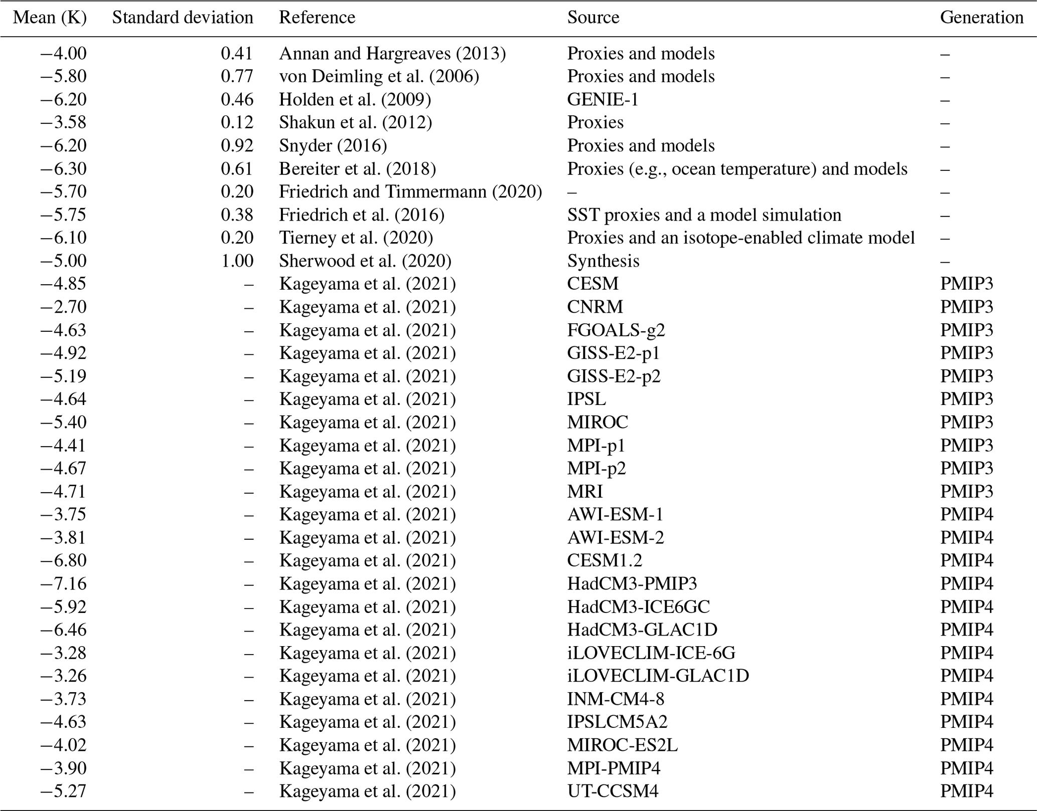
Figure 6 illustrates how the posterior distribution of ΔT depends on prior beliefs about the nature and quality of the published literature assessing it.

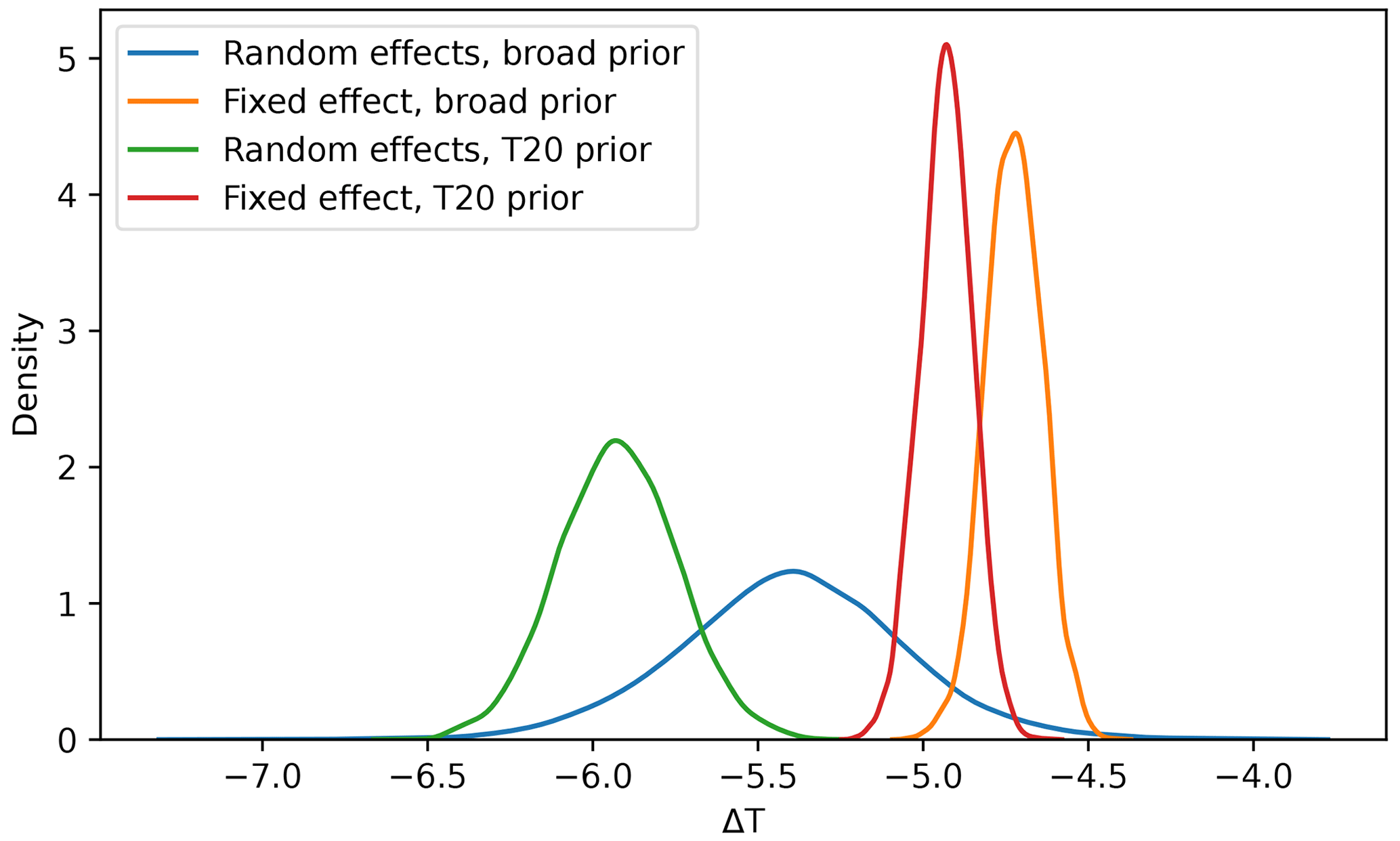
Figure 6 How cold was the Last Glacial Maximum? The answer depends on your prior beliefs about the cooling and the literature. Shown are posterior distributions for the LGM cooling (ΔT), assuming a random-effects model with a broad prior (blue line) or a T20 prior (green) on the mean or assuming a fixed-effects model with a broad prior (orange line) or a T20 prior (red line) on the mean.

Consider, for example, a random-effects model in which we place broad priors on the mean $\mathit{\mu }\sim N(\mathrm{0},\mathrm{100})$ and the inter-study standard deviation $\mathit{\tau }\sim U(\mathrm{0},\mathrm{100})$. With these prior assumptions, 90 % of the resulting posterior density for μ (the true value of ΔT) lies between −5.9 and −4.8 K. Assuming that there is no inter-study spread (i.e., assuming that τ is zero with zero uncertainty, corresponding to a fixed-effects model) would yield an estimate of ΔT that is 90 % likely to be between −4.8 and −4.5 K. This much narrower (and warmer) estimate results from the extremely restrictive prior belief that every study, regardless of method, targets the same underlying ΔT value and would yield the same results if performed perfectly and with adequate data. Similarly, we might set the prior on μ using the result of a single published study (for example, ΔT from T20). Combined with a broad uniform prior on the inter-study spread, this results in an 90 % posterior density estimate ranging from −6.2 to −5.6 K. If, however, we adopt the restrictive fixed-effects model, the T20 study is merely treated as an outlier and fails to substantially move the posterior distribution toward cooler values of ΔT (red line), even when using the T20 prior.

7.1.1 Recommendations

Unavoidable subjective decisions about the evidence can be made explicit by adopting a random-effects meta-analysis. This requires the specification of priors on the inter-study spread (τ) and the overall mean (Y). Our recommendation is that the organizers of community assessments choose and clearly specify these priors, rather than allowing individual experts to choose their own.

7.2 Handling model uncertainty

As shown in Sect. 4, the constraints placed on climate sensitivity by multiple lines of evidence depend on the model(s) used to interpret that evidence. This means that the design of each expert assessment must be explicit regarding its interpretive models. As the assessment is planned, it is crucial to arrive at a consensus on credible interpretive models for the evidence. For example, one possible model for the Last Glacial Maximum might incorporate the parameters α (representing state dependence), ξ (representing the difference between long-term equilibrium feedbacks for the LGM and target quasi-equilibrium feedbacks for doubled CO₂), and Δλ_LGM (representing sea surface pattern differences between the LGM and doubled CO₂), resulting in the following equation:

$$\mathrm{\Delta }T={\displaystyle \frac{-\mathrm{\Delta }F}{\frac{\mathit{\lambda }+\mathrm{\Delta }{\mathit{\lambda }}_{\mathrm{LGM}}}{\mathrm{1}+\mathit{\xi }}+\frac{\mathit{\alpha }}{\mathrm{2}}\mathrm{\Delta }T}}.$$

Given a model, experts may then be asked to specify their prior beliefs about each parameter. If an expert disagrees with the inclusion of a parameter in the model, they would be free to set a prior that is very narrowly clustered around zero.

If consensus cannot be reached on a particular model, then we suggest that the planners for any assessment arrive at a list of candidate models (M₁…M_K). The aggregate posterior can then be taken as a weighted average over different models as follows:

$$\begin{array}{}\text{(11)}& P\left(\mathrm{\Theta }\right|Y)=\sum _{k=\mathrm{1}}^K{w}_{k}P(\mathrm{\Theta }|M_k,Y).\end{array}$$

Here, $\left(\mathrm{\Theta }\right|M_k,Y)$ is the posterior obtained using the model M_k to interpret the evidence (Y).

The weights reflect how well the model fits the data and are given by

$$\begin{array}{}\text{(12)}& w_k=P\left(M_k\right|Y)={\displaystyle \frac{P\left(Y\right|M_k\left)P\right(M_k)}{{\sum }_{k=\mathrm{1}}^{K}P\left(Y\right|M_k\left)P\right(M_k)}}.\end{array}$$

The term P(M_k|Y) is the model evidence (Eq. 8), as discussed in Sect. 6.2. These weights, and hence the combined posterior, depend on the set of priors (P(M_k)) we place on the correctness of each model. If an assessment allows for experts to use one of multiple models, it is imperative to specify assessment-wide priors for these models upfront.

7.2.1 Recommendations

We recommend that organizers of community assessments clearly specify a single interpretive model for the evidence used. If this is not possible, organizers should specify a list of possible candidate models (M_k) and a prior (P(M_k)) for each candidate model. The resulting estimate will then be a weighted average over the models.

7.3 Expert elicitation via priors

Finally, it is necessary to quantify the degree of preexisting knowledge and/or beliefs through the use of prior distributions. This is where a wide variety of expert opinions may be usefully incorporated into an assessment.

However, we require consistent ways to aggregate the judgments of multiple experts. In theory, sufficient evidence should lead to a high degree of agreement, even if different experts begin the analysis with very different priors. Figure 7a shows the priors placed on the parameter λ by two hypothetical experts. Expert A (solid red line) believes that the feedback parameter is less negative than Expert B (solid blue line) thinks it is and is even open to the idea that it might be positive. The dashed red and blue lines show both experts' posteriors, updated using the evidence presented in S20. While the experts began their analysis with differing opinions, the weight of the evidence has updated their understandings, and they now agree about the feedback parameter (λ).

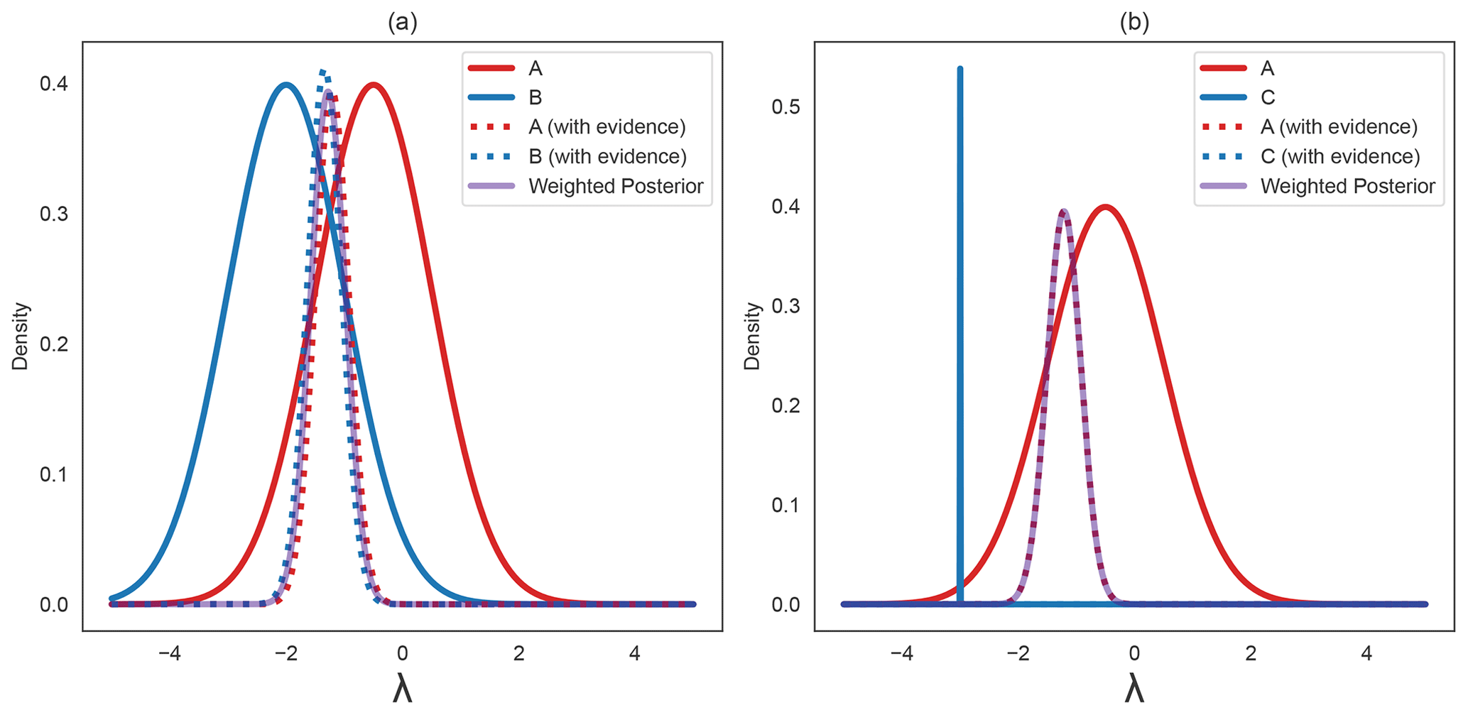
Figure 7 (a) Experts A (solid red line) and B (solid blue line) begin with different priors on λ. The evidence presented in S20 updates these priors, and the resulting posteriors are nearly identical (dotted red and blue lines). The purple line shows the weighted posterior. (b) Experts A (solid red line) and C (solid blue line) begin with different priors on λ, but Expert C's prior is very narrowly peaked. The evidence presented in S20 updates these priors, but the posteriors remain very different (dotted red and blue lines). The purple line shows the weighted posterior, which is almost identical to Expert A's posterior.

However, some experts may not be as open-minded as Experts A and B. Expert C (blue line in Fig. 7b believes that the feedback parameter is strongly negative. Moreover, they are extremely confident in this: their prior distribution is very narrowly peaked around a value of $\mathit{\lambda }=-\mathrm{3}$ W m⁻² K⁻¹. Expert C's confidence remains unshaken by the evidence presented in S20, and their posterior remains nearly identical to their prior beliefs. How should an assessment handle such excessively confident experts, whose beliefs appear to be unshaken by any reasonable amount of evidence?

Consider an assessment in which N experts each specify a set of priors (P_i(θ)), where i=1…N. A reasonable aggregate prior might then be a linear combination of the individual expert priors, expressed as

$$\begin{array}{}\text{(13)}& P\left(\mathit{\theta }\right)=\sum _{i=\mathrm{1}}^N{a}_i{P}_i\left(\mathit{\theta }\right).\end{array}$$

The aggregate posterior is therefore a weighted average of the individual expert posteriors, given by

$$\begin{array}{}\text{(14)}& P(\mathit{\theta },Y)=\sum _i{\stackrel{\mathrm{̃}}{a}}_i{P}_i\left(\mathit{\theta }\right|i,Y),\end{array}$$

where

$$\begin{array}{}\text{(15)}& {\stackrel{\mathrm{̃}}{a}}_i={\displaystyle \frac{a_i\int P\left(Y\right|\mathit{\theta }\left)P_i\right(\mathit{\theta })\mathrm{d}\mathit{\theta }}{{\sum }_{i=\mathrm{1}}^N{a}_i\int P\left(Y\right|\mathit{\theta }\left)P_i\right(\mathit{\theta })\mathrm{d}\mathit{\theta }}}.\end{array}$$

This method introduces N new parameters, representing the prior weight (a_i) we assign to each expert's judgment. This is a far easier task than setting priors on models (as discussed in Sect. 7.2) because it requires no physical understanding but rather a belief about the quality of each expert's initial beliefs. We recommend weighting each expert equally by setting $a_{\mathrm{1}}=a_{\mathrm{2}}=\mathrm{\dots }{a}_N=\frac{\mathrm{1}}{N}$, in which case the posterior weight becomes

$$\begin{array}{}\text{(16)}& {\stackrel{\mathrm{̃}}{a}}_i={\displaystyle \frac{\int P\left(Y\right|\mathit{\theta }\left)P_i\right(\mathit{\theta })\mathrm{d}\mathit{\theta }}{{\sum }_{i=\mathrm{1}}^N\int P\left(Y\right|\mathit{\theta }\left)P_i\right(\mathit{\theta })\mathrm{d}\mathit{\theta }}}.\end{array}$$

The purple line in Fig. 7a shows the resulting aggregate posterior given Expert A and Expert B's priors. Because these experts are similarly able to update their priors, the weighting process has no effect on the outcome. However, the weighted average of Expert A and Expert C's posteriors, indicated by the purple line in Fig. 7b, is similar to Expert A's posterior distribution. The narrowness of Expert C's prior causes their posterior distribution to be down-weighted in the weighted average. We suggest this as an effective strategy for handling inflexible or extremely anomalous expert opinions.

7.3.1 Recommendations

We recommend eliciting expert judgment in a systematic way by allowing experts to specify priors on predetermined model parameters. The analysis can then be performed using a single aggregate posterior, calculated as the weighted average of individual expert posteriors.

8 Conclusions

Here, we have presented three sources of uncertainty that enter into estimates of climate sensitivity, which can be summarized as three sets of questions as follows. First, what evidence should we use to constrain climate sensitivity, how do we decide what counts as evidence, and how should we handle estimates that disagree or conflict with each other? Second, what interpretive model should we use to relate the evidence to climate sensitivity, and what parameters are required? Third, what prior knowledge of these parameters is appropriate and should be included? We then propose a strategy to make the role of expert judgment in subsequent assessments fairer and more transparent. The advantage of this strategy, combining Bayesian meta-analysis and Bayesian model averaging, is that it can incorporate newly published data and is easily expanded to handle uncertainties at multiple levels.

There is no limit to the number of nested levels we could theoretically use within a Bayesian hierarchical model: the prior for radiative forcing from ice sheets, for example, can be updated using a global ice sheet reconstruction, which itself is constrained by individual geological measurements. Similarly, a prior on ocean heat uptake (ΔN) or historical warming (ΔT) can be updated as new measurements become available. However, to remain tractable, every project must truncate the hierarchy at some finite level. In practice, this means treating the posteriors that arise from observational, general-circulation-model (GCM), or paleoclimate studies as evidence; where we draw the line between evidence and parameters sets the bounds of our analysis.

As a result, we propose a framework in which experts are required to specify their choices at clearly defined decision points. Once priors are specified, the model and evidence will update them accordingly, arriving at a new, aggregate consensus posterior. We review this framework here.

Somewhat obviously, experts' beliefs about the data are based on their prior beliefs, updated by the evidence. But how experts interpret and use that evidence depends on the subjective choices they make – i.e., what counts as a study or evidence? How should we best compare estimates derived from proxies or observations with estimates from GCMs? Should some studies receive more weight than others? In our framework, experts must make judgments about the evidence by asking the following questions:

1. What is your informed belief about the evidence? (For example, what is your prior on μ?)

2. What is your belief about the published literature? (What is your prior on τ?)

Second, we suggest taking the choice of model out of individual participants' hands to the greatest extent possible. Ideally, assessment planners should arrive at a single model and set of parameters on which experts may specify their priors. If not, they should arrive at a list of candidate models, specify firm prior beliefs about these models, and perform Bayesian model averaging over the posteriors of individual experts, which will depend on the model they use.

Third, once a model is specified, experts should specify their prior beliefs about the parameters of that model.

The results presented here are meant to begin, rather than end, a conversation. The beauty of Bayesian methods is that we can allow new evidence to update our existing knowledge. As climate researchers gear up for the next generation of model intercomparison projects and assessments, it is important to consider how these new results will be integrated with existing knowledge. Our methods presented here allow for new discoveries to advance our understanding, ultimately narrowing the bounds of climate sensitivity and informing future research and decision-making.

Appendix A: Exact forms of integrals

To estimate the likelihood of the evidence (ΔT and ΔF) given the simple energy balance model, we integrate the joint probability distribution (𝒥(ΔT,ΔF)) over the curve (C) using the following model:

$$\begin{array}{}\text{(A1)}& P\left(Y\right|\mathit{\lambda },M_{\mathrm{0}})=\underset{C}{\int }\mathcal{J}(\mathrm{\Delta }T,\mathrm{\Delta }F)\mathrm{d}s.\end{array}$$

C can be parameterized as

$$\begin{array}{}\text{(A2)}& \mathbf{r}\left(t\right)=t\widehat{i}+-\mathit{\lambda }t\widehat{j},\end{array}$$

and the integral is then given by

$$\begin{array}{}\text{(A3)}& \begin{array}{rl}P\left(Y|\mathit{\lambda },M_{\mathrm{0}}\right)& =\underset{-\mathrm{\infty }}{\overset{\mathrm{\infty }}{\int }}\mathcal{J}\left(\mathbf{r}\right(t\left)\right)\left|\right|{\mathbf{r}}^{\prime }\left(t\right)\left|\right|\mathrm{d}t\\ & =\underset{-\mathrm{\infty }}{\overset{\mathrm{\infty }}{\int }}\mathcal{J}(t,-\mathit{\lambda }t)\sqrt{\mathrm{1}+{\mathit{\lambda }}^{\mathrm{2}}}\mathrm{d}t.\end{array}\end{array}$$

In the case where ΔT and ΔF are Gaussian and independent (with the means μ_T and μ_F and the standard deviations σ_T and σ_F, respectively), the likelihood has an exact analytic form, substantially speeding up its computation. This form is expressed as

$$\begin{array}{}\text{(A4)}& P\left(Y\right|\mathit{\lambda },M_{\mathrm{0}})=C{\left({\displaystyle \frac{\mathrm{2}\mathit{\pi }}{A}}\right)}^{\mathrm{1}/\mathrm{2}}\exp \left({\displaystyle \frac{B^{\mathrm{2}}}{\mathrm{2}A}}\right),\end{array}$$

where

$$\begin{array}{c}{\displaystyle }C={\displaystyle \frac{\sqrt{\mathrm{1}+{\mathit{\lambda }}^{\mathrm{2}}}}{\mathrm{2}\mathit{\pi }{\mathit{\sigma }}_T{\mathit{\sigma }}_F}}\exp \left({\displaystyle \frac{{\mathit{\mu }}_T^{\mathrm{2}}}{{\mathit{\sigma }}_T^{\mathrm{2}}}}+{\displaystyle \frac{{\mathit{\mu }}_F^{\mathrm{2}}}{{\mathit{\sigma }}_F^{\mathrm{2}}}}\right),\\ {\displaystyle }A={\displaystyle \frac{\mathrm{1}}{{\mathit{\sigma }}_T^{\mathrm{2}}}}+{\displaystyle \frac{{\mathit{\lambda }}^{\mathrm{2}}}{{\mathit{\sigma }}_F^{\mathrm{2}}}},\\ {\displaystyle }B={\displaystyle \frac{{\mathit{\mu }}_T}{{\mathit{\sigma }}_T^{\mathrm{2}}}}-{\displaystyle \frac{\mathit{\lambda }{\mathit{\mu }}_F}{{\mathit{\sigma }}_F^{\mathrm{2}}}}.\end{array}$$

In the case of a three-dimensional space (as with the historical evidence), the curve (C) defines a plane rather than a line, and we have

$$\begin{array}{}\text{(A5)}& \begin{array}{rl}& P\left(Y\right|\mathit{\lambda })\propto \underset{C}{\int }\mathcal{J}(\mathrm{\Delta }T,\mathrm{\Delta }F,\mathrm{\Delta }N)\mathrm{d}S\\ & =\int \int \mathcal{J}\left(\mathit{r}(u,v)\right)\left|\right|r_u\times r_v\left|\right|\mathrm{d}u\mathrm{d}v,\end{array}\end{array}$$

where

$$\begin{array}{}\text{(A6)}& \mathit{r}=u\widehat{i}+v\widehat{j}+(\mathit{\lambda }u+v)\widehat{k}.\end{array}$$

Appendix B: Likelihood vs. probability

We note that this method is distinct from estimating λ as the ratio of the distributions ΔF and ΔT. This is due to a conceptual difference between probability and likelihood. Constructing the likelihood answers the following question: (1) how likely is a particular hypothesis (in this simple case, a particular value of λ) given the evidence? This is a fundamentally different question from the following: (2) what is the probability density function of the ratio $-\mathrm{\Delta }F/\mathrm{\Delta }T$? The first question involves fixing a putative value of λ, which is not treated as a random variable. The second question treats λ as a random variable. Mathematically, this is reflected in the difference between (1) a line integral over the curve $y=-\mathit{\lambda }x$,

$$P(x,y|\mathit{\lambda })=\underset{C}{\int }{P}_{xy}(x,y)\mathrm{d}s=\underset{-\mathrm{\infty }}{\overset{\mathrm{\infty }}{\int }}{P}_{xy}(x,-\mathit{\lambda }x)\sqrt{\mathrm{1}+{\mathit{\lambda }}^{\mathrm{2}}}\mathrm{d}x,$$

and (2) the ratio distribution of the random variable $\mathit{\lambda }=-y/x$,

$$P_{\mathit{\lambda }}\left(\mathit{\lambda }\right)=\underset{-\mathrm{\infty }}{\overset{\mathrm{\infty }}{\int }}{P}_{xy}(x,-\mathit{\lambda }x)\left|x\right|\mathrm{d}x.$$

We use the ratio distribution (b) to estimate S once we have the posterior probability density function (PDF) for λ. This is because we treat S as the ratio of two random variables, $F_{\mathrm{2}\times {\mathrm{CO}}_{\mathrm{2}}}$ and λ.

Appendix C: Correlations between $F_{\mathrm{2}\times {\mathrm{CO}}_{\mathrm{2}}}$ and ΔF

CO₂ emissions are the primary contributor to present-day radiative-forcing change relative to preindustrial concentrations. Atmospheric concentrations of CO₂ were lower in the Last Glacial Maximum. This means that the forcing term (ΔF) used as evidence in the LGM and historical periods is correlated with the forcing corresponding to doubled CO₂. For visual clarity, we neglect this correlation in this paper. To take it into account, we can write the simple energy balance model as

$$\mathrm{\Delta }N=\mathrm{\Delta }{F}^{\prime }+\mathit{\beta }{F}_{\mathrm{2}\times {\mathrm{CO}}_{\mathrm{2}}}+\mathit{\lambda }\mathrm{\Delta }T.$$

In this case, the likelihood $P\left(E\right|\mathit{\lambda },F_{\mathrm{2}\times {\mathrm{CO}}_{\mathrm{2}}})$ is defined as the integral of the joint probability distribution of the evidence (E) over the curve defined by the model. Following S20, we can then calculate S by changing the variables and marginalizing over $F_{\mathrm{2}\times {\mathrm{CO}}_{\mathrm{2}}}$ as follows:

$$\begin{array}{rl}P\left(S\right|E)=& \int P\left({\mathit{\lambda }}^{\prime },F_{\mathrm{2}\times {\mathrm{CO}}_{\mathrm{2}}}^{\prime }|E\right)\\ & \mathit{\delta }\left(S-F_{\mathrm{2}\times {\mathrm{CO}}_{\mathrm{2}}}^{\prime }/{\mathit{\lambda }}^{\prime }\right){\left(\partial S/\partial {\mathit{\lambda }}^{\prime }\right)}^{-\mathrm{1}}\\ & {\left(\partial S/\partial F_{\mathrm{2}\times {\mathrm{CO}}_{\mathrm{2}}}^{\prime }\right)}^{-\mathrm{1}}\mathrm{d}F{{}^{\prime }}_{\mathrm{2}\times {\mathrm{CO}}_{\mathrm{2}}}\mathrm{d}{\mathit{\lambda }}^{\prime }.\end{array}$$

Practically, we can draw samples of λ and $F{{}^{\prime }}_{\mathrm{2}\times {\mathrm{CO}}_{\mathrm{2}}}$ from the joint posterior distribution and use these to calculate a posterior distribution for S. This correlation contributes very little to the results; when taking it into account, we obtain similar ranges for S as when we neglect it.