Inconclusive early warning signals for Dansgaard-Oeschger events across Greenland ice cores

The Dansgaard-Oeschger (DO) events of past glacial episodes provide an archetypical example of abrupt climate shifts and are discernible, for example, in oxygen isotope ratios from Greenland ice core records. The causes and mechanisms underlying these events are still subjects of ongoing debate. It has previously been hypothesised that DO events may be triggered by bifurcations of mechanisms operating at decadal time scales, as indicated by a significant number of early warning signals (EWS) in the high-frequency variability of records from the North Greenland Ice Core Project (NGRIP). Here, we re-evaluate the presence of EWS by employing indicators based on critical slowing down (CSD) and wavelet analysis and conduct a systematic methodological robustness test. Our findings reveal fewer significant EWS than previous studies, yet their numbers are significant for some of the indicators estimating changes in variability. Additionally, a comparison of different Greenland ice core records also shows consistency for these same EWS estimators preceding a small selection of events in records with high temporal resolution. While those indicators might represent changes in a common climate background, we cannot rule out that signals specific to the different ice core locations are captured. Nevertheless, the numbers of detected EWS are not significant for most ice core records as well as for estimators of correlation times when considered on their own, which were found to be less consistent. Based on these inconclusive results it is not possible to constrain mechanisms underlying the DO events. Instead, our results highlight the complexities and limitations of applying early warning signals to paleoclimate proxy data.

1 Introduction

The last glacial period, spanning from approximately 110 000 to 12 000 years before the year 2000 (yr b2k), was marked by aperiodic and abrupt climate changes, called Dansgaard-Oeschger (DO) events (Dansgaard et al., 1982; Johnsen et al., 1992; Dansgaard et al., 1993). They are characterised by rapid warming of 5 to 16.5 °C (Kindler et al., 2014) over a few decades from colder conditions during Greenland Stadials (GS) to milder ones in Greenland Intersadials (GI), followed by more gradual cooling over centuries or millennia back to GS (Dansgaard et al., 1982; Johnsen et al., 1992; Rasmussen et al., 2014). DO events were first discovered, and are most evident, in records of oxygen isotope ratios δ¹⁸O from Greenland ice cores (Dansgaard et al., 1993; North Greenland Ice Core Project members et al., 2004), which are commonly used as local temperature proxies. Similar transitions, however, can also be seen in other paleoclimate records including terrestrial archives such as Loess decompositions or speleothems representing the activity of the tropical monsoon systems (Rousseau et al., 2017; Corrick et al., 2020). While the strongest expression of DO events was seen in the North Atlantic region (Dansgaard et al., 1982; Johnsen et al., 1992; Dansgaard et al., 1993), they had strong impacts on climate patterns across the globe (e.g. Blunier and Brook, 2001; Cruz et al., 2005; Wagner et al., 2010; Fohlmeister et al., 2023).

Despite decades of research, the physical processes behind DO events remain debated. The initially proposed periodicity of approximately 1470 years suggested that astronomical forces and centennial-scale solar cycles might have influenced these events (Schulz, 2002), but later studies (Ditlevsen et al., 2007) have indicated that this periodicity might be misleading. Instead, DO variability is often associated with changes in the Atlantic Meridional Overturning Circulation (AMOC), characterised by a weak or shut-off AMOC during GS and strong overturning during GI (see e.g. Lynch-Stieglitz, 2017). However, the specific underlying mechanisms are still not fully understood. Such changes could be driven by external forces (Ganopolski and Rahmstorf, 2001; Knorr and Lohmann, 2003; Zhang et al., 2014, 2017) such as atmospheric carbon dioxide levels (Banderas et al., 2012; Vettoretti et al., 2022), freshwater discharges from the Laurentide ice sheets (Boers et al., 2022), or volcanic cooling (Lohmann and Svensson, 2022). Nevertheless, shifts in the AMOC and δ¹⁸O values in Greenland could also arise from unforced self-oscillation mechanisms (Peltier and Vettoretti, 2014) that are influenced by internal ocean dynamics (Klockmann et al., 2020) and rapid changes in the North Atlantic sea ice (Dokken et al., 2013; Petersen et al., 2013; Boers et al., 2018). The latter is supported by recent advances in comprehensive climate models (e.g. Sakai and Peltier, 1997; Vettoretti and Peltier, 2018; Klockmann et al., 2020; Buizert et al., 2024), which now depict DO-like events as such oscillations influenced by interactions among sea ice, atmospheric dynamics, and the AMOC (see Malmierca-Vallet et al., 2023 for a review).

DO events provide compelling evidence that abrupt climate transitions over short timescales, relevant for human societies, have occurred in the Earth’s past climate system. As such, DO events can be considered archetypes of abrupt climate changes (Boers et al., 2022), which may be caused by crossing system tipping points (TPs). TPs are critical thresholds where a small perturbation can significantly and non-linearly alter the state or development of a system, often abruptly and/or irreversibly (Lenton et al., 2008), and are a source of growing concern with regards to the potential consequences of ongoing anthropogenic warming. Depending on the mechanisms behind a TP, they can be classified as noise-induced (N-tipping) if a TP is crossed due to internal variations in the system, bifurcation-induced (B-tipping) if tipping occurs by approaching a bifurcation, due to changes in a forcing parameter, where the current state loses stability and the system moves to another stable state, or rate-induced (R-tipping) if the tipping is not associated with either bifurcation or noise, but is rather caused by rapid changes in the forcing parameter (Ashwin et al., 2012).

Since the physical mechanisms behind DO events are yet to be clarified, the debate whether they were caused by changes in an external forcing or through unforced processes, or in other words, the question whether DO events can be considered as examples of N-, or B-tipping is still ongoing. Analyses of dust (Ca²⁺) records from different Greenland ice core sites suggest that DO events might not be purely noise-induced (Lohmann, 2019) and reveal a possible bifurcation structure (Riechers et al., 2023b). Studies of the δ¹⁸O record from the North Greenland Ice Core Project (NGRIP, North Greenland Ice Core Project members et al., 2004), on the other hand, indicate that these transitions are predominantly noise-induced (Lohmann and Ditlevsen, 2019) and don't exhibit an underlying bifurcation (Riechers et al., 2023b). Recent conceptual models also propose different tipping mechanisms for DO events, such as a cascade of tipping points lead by R-tipping of the AMOC due to rapid sea ice changes (Lohmann et al., 2021), and noise-induced transitions from GS to GI due to fast intermittent anomalies acting on the sea ice cover (Riechers et al., 2023a).

For systems approaching B-tipping, quantitative indicators that signal the proximity of the system to the TP, so-called Early Warning Signals (EWS), might potentially be found before the transition. Most common EWS are based on Critical Slowing Down (CSD): As a system approaches a TP, the stability of the state decreases and its basin of attraction widens. This is characterised by increasing fluctuation levels and longer correlation times, hence variance V and autocorrelation α₁ are expected to increase in the observed signal (Dakos et al., 2008; Scheffer et al., 2009; Ditlevsen and Johnsen, 2010; Boers, 2021). The restoring rate λ yields another indicator of CSD, which can be used to quantify the stability of a system (Held and Kleinen, 2004; Rypdal and Sugihara, 2019; Boers, 2021) (Sect. 2.2). To capture stability changes in subcomponents of the system operating on specific timescales, EWS might be constrained to certain frequency bands of the signal. Accordingly, wavelet-based estimators have been proposed by Rypdal (2016) and further applied in Boers (2018) for DO events. The scale-averaged wavelet coefficient ${\widehat{w}}^{\mathrm{2}}$ is used to estimate variance, whilst the local Hurst exponent ${\widehat{H}}^{\text{loc}}$ gives an estimation of correlation times (Sect. 2.2). In contrast to that, EWS are not expected to occur for purely noise-induced transitions.

While rigorous theory exists for EWS in certain low-dimensional systems (Kuehn, 2011), for instance in analogy with the Ornstein–Uhlenbeck process (see e.g. Ditlevsen and Johnsen, 2010; Boers, 2021), the predictive power of EWS might be limited for complex and high-dimensional natural systems, such as the Earth’s climate (Boers et al., 2022). Even if tipping is due to a bifurcation, EWS might not be found due to multiple factors, such as the complexity of the underlying system with interactions across variables that might mask EWS (Morr and Boers, 2024), or an underlying complex bifurcation structure that may not cause any CSD-based EWS (Morr et al., 2024). Furthermore, the apparent presence of EWS does not automatically imply that a system approaches a bifurcation since the observed fluctuations may be caused by something else or purely arise by chance and yield false positives (Boers, 2021). Thus, it is typically assumed that a transition is not entirely noise-induced if EWS are observed preceding a transition. It can also be helpful to look at multiple EWS indicators simultaneously: Although variance increases for a system with increasing noise levels that is not approaching a bifurcation, its autocorrelation remains constant (Ditlevsen and Johnsen, 2010; Smith et al., 2023). Despite these shortcomings, the presence or absence of EWS for DO events can give an indication of the underlying tipping mechanisms.

Even though the background climate during the last glacial period and today are different, similar abrupt transitions as those during DO events may be triggered during current and future warming, where the transition may occur much faster than the change in forcing. Early warning signals have received a lot of attention in recent years and they are expected to precede potential future tipping points, e.g., in the polar ice sheets or the AMOC. Climate model studies (van Westen et al., 2024) and analyses of observational data (Boers, 2021; Ditlevsen and Ditlevsen, 2023) have found EWS for a possible future destabilisation of the AMOC. A potential future weakening or shut-down of the AMOC would have severe impacts on the global climate and could lead to cooling over the Northern Hemisphere (Stouffer et al., 2006; Drijfhout, 2015; Jackson et al., 2015). Hence, future changes might be more comparable to past transitions from GI to GS, rather than DO events with changes from GS to GI, during the last glacial period. Past GI-GS transitions, as those shown in Fig. 2, occurred more gradually than the abrupt DO events and have consequently received less attention regarding possible EWS. Nevertheless, the presence of EWS for past abrupt transitions is the only empirical evidence that similar precursors may be found in observations before future tipping.

While most previous work on EWS for DO events has focused on the abrupt warmings, one study (Mitsui and Boers, 2024) focused on cooling events from GI to GS during the same time period and found robust CSD-based EWS across δ¹⁸O and dust records from three Greenland ice cores. Several earlier studies have looked for EWS for DO events in δ¹⁸O records from the North Greenland Ice Core Project (NGRIP, North Greenland Ice Core Project members et al. (2004)) with mixed results. Considering the ensemble average of several DO events, Cimatoribus et al. (2013) find weak but significant CSD-based EWS, whereas Rypdal (2016) later demonstrated that such an average does not yield significant EWS if only the GS preceding DO events are considered. When looking for indications of CSD for individual DO-events across the entire frequency spectrum, Ditlevsen and Johnsen (2010) found no significant EWS preceding any of the 17 events considered there. In contrast to that, Myrvoll-Nilsen et al. (2025) found significant increases for several DO events of the autocorrelation parameter during the preceding GS using a new statistical approach.

Rypdal (2016) limited the search for EWS to high-frequency fluctuations, motivated by the hypothesis that processes operating at time scales shorter than a century are responsible for the rapid, decadal-scale DO transitions. If these are caused by bifurcations, EWS might be detectable in high-frequency bands but masked by low-frequency variability if the entire spectrum is taken into account. To further study such high-frequency fluctuations for individual transitions in the periodicity band between 40 and 60 years, the wavelet-based indicators ${\widehat{w}}^{\mathrm{2}}$ and ${\widehat{H}}^{\text{loc}}$ have been introduced. The author finds some significant EWS for both indicators individually and simultaneously.

A subsequent study (Boers, 2018) re-evaluated the hypothesis of Rypdal (2016) using the raw NGRIP record (North Greenland Ice Core Project members et al., 2004; Gkinis et al., 2014) interpolated to a higher temporal resolution of 5 years instead of the 20 years temporal resolution previously used. There, a significant amount of significant increases in the variance of the 100-year high-pass filtered signal, as well as simultaneous significant increases in variance and autocorrelation is found during GS. Analysis of various frequency bands between 10 and 110 years reveals most wavelet-based EWS in a scale range of 10 to 50 years, where a significant amount of significant EWS is found for ${\widehat{w}}^{\mathrm{2}}$, ${\widehat{H}}^{\text{loc}}$, and both occurring simultaneously. These results suggested that DO events might have occurred due to B- rather than N-tipping.

Previous EWS analyses for DO warming transitions have all been conducted on the δ¹⁸O record from the NGRIP ice core in various temporal resolutions but other available δ¹⁸O records from other ice cores (Fig. 1), that clearly exhibit the same DO events (Rasmussen et al., 2014) as it can be seen in Fig. 2, have not been taken into account. This raises the question whether the high-frequency δ¹⁸O variability from different Greenland ice core records is comparable during GS before transitions and whether similar EWS can be found across different records and temporal resolutions.

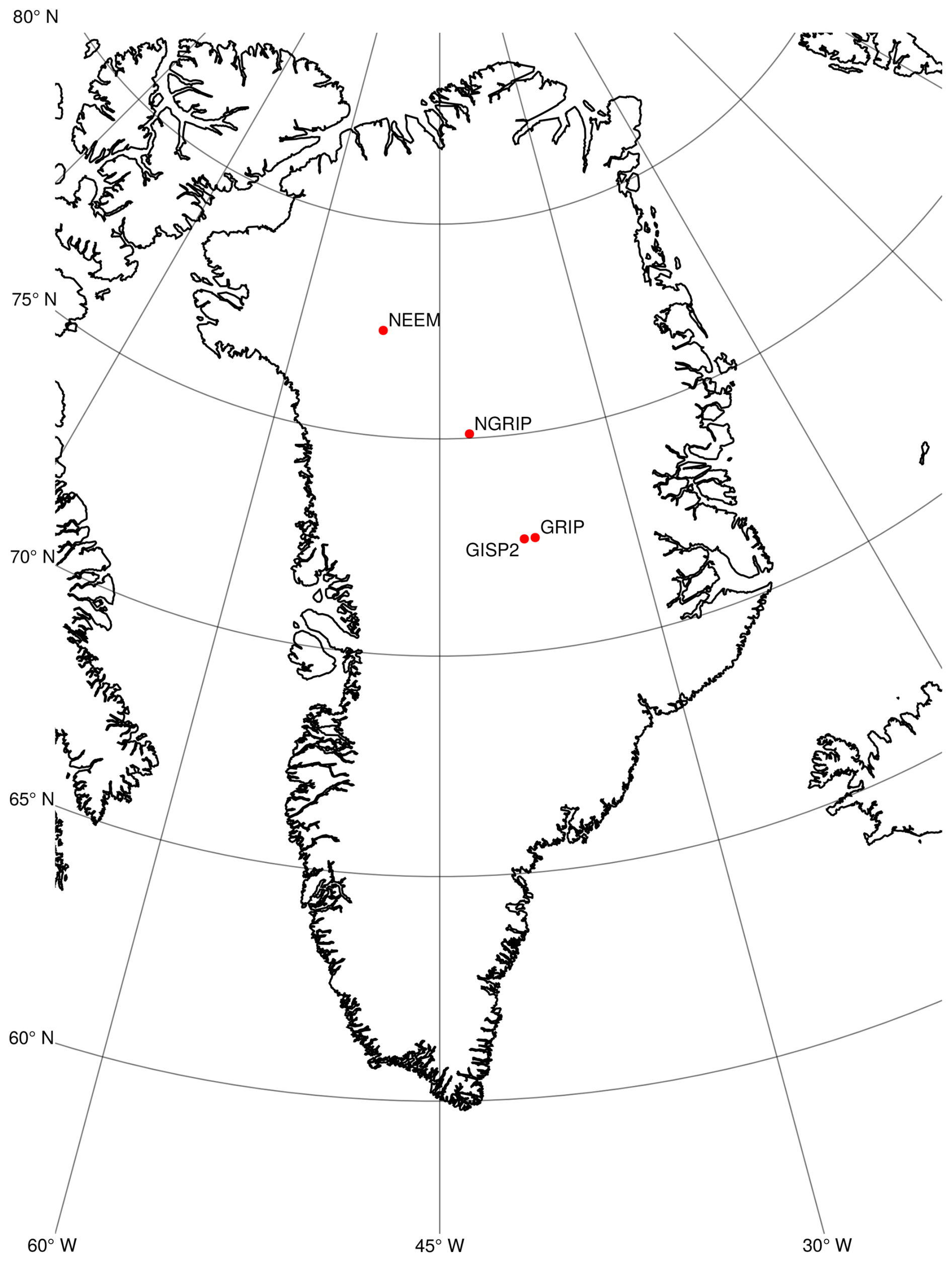
Figure 1 Map of Greenland with the locations of the deep ice core drilling sites GRIP (72.58° N, 37.64° W), GISP2 (72.58° N, 38.48° W), NGRIP (75.10° N, 42.32° W), and NEEM (77.45° N, 51.06° W) marked in red.

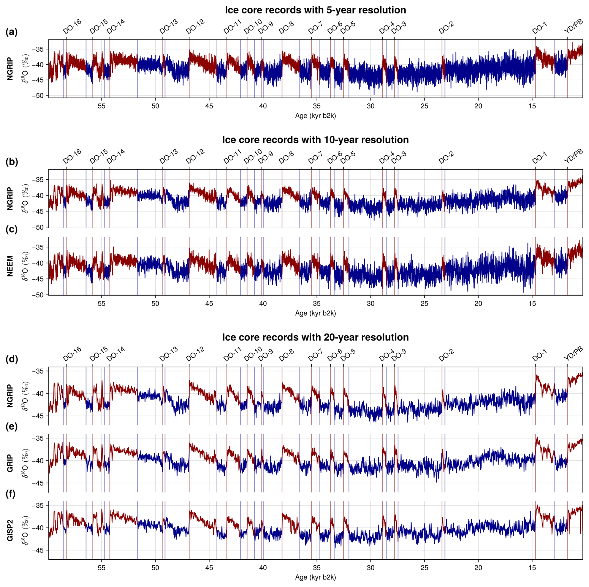
Figure 2 Greenland δ¹⁸O proxy records from NGRIP in 5- (a), 10- (b), and 20-year (d) resolution, NEEM in 10-year resolution (c), GRIP (e), and GISP2 (f) in 20-year resolution. Time series during GS studied here are shown in blue, their onsets are marked with blue vertical lines. DO events and the YD/PB transition are marked by the red vertical lines and define the onsets of GI, drawn in red.

Here we re-evaluate the results from Boers (2018) across multiple Greenland ice cores (Sect. 3.3). We conduct a systematic comparison of EWS during GS before DO events for a total of six δ¹⁸O time series from four ice core sites in three different temporal resolutions (see Figs. 1, 2, Table 1, and Sect. 2.1) to assess whether the observed high-frequency fluctuations prior to DO events 1–16 (counting from younger to older events, see Fig. 2, Svensson et al., 2008) and the Younger Dryas-Preboreal transition (YD/PB, at approx. 11 700 yr b2k, Svensson et al., 2008) stem from a common climate signal or could have been caused by other factors. The early warning indicators considered, variance V, lag − 1 autocorrelation coefficient α₁, wavelet fluctuation level ${\widehat{w}}^{\mathrm{2}}$, and the local Hurst exponent ${\widehat{H}}^{\text{loc}}$, are the same as used by Boers (2018), where we apply some modifications to the methods presented there (see Sect. 2.5). Moreover, we evaluate the robustness of EWS on these methodological changes, i.e. different choices in significance testing, EWS estimation, and data preprocessing for the NGRIP record with 5-year temporal resolution (Sect. 3.1), for which we also estimate the restoring rate λ. To circumvent potential interpolation effects, we further conduct a similar study on the raw NGRIP record applying an approach adapted specifically for the analysis of irregularly sampled time series (Sect. 3.2).

2 Methods

2.1 Data and preprocessing

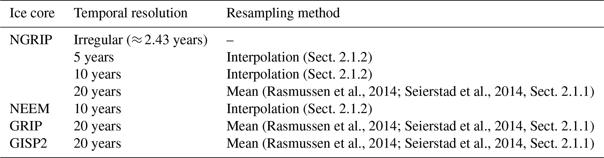
We consider all available δ¹⁸O records from Greenland ice cores between 59 920 and 10 295 yr b2k on the associated annual-layer counted Greenland Ice-Core Chronology 2005 (GICC05, Rasmussen et al., 2006; Andersen et al., 2006; Svensson et al., 2006) with a temporal resolution of at least 20 years. An overview of these records is given in Table 1.

Rasmussen et al., 2014; Seierstad et al., 2014Rasmussen et al., 2014; Seierstad et al., 2014Rasmussen et al., 2014; Seierstad et al., 2014

Table 1 Overview of δ¹⁸O records from Greenland ice cores considered in this study. Regular temporal resolutions are obtained by the corresponding resampling methods.

For the estimation of CSD-based EWS V and α₁, we use the 100-year high-pass filtered data of the normalised time series. This is achieved by applying a Chebychev Type-I high-pass filter with cutoff at 100 years.

2.1.1 Ice core data in 20-year resolution

The three δ¹⁸O records from NGRIP (North Greenland Ice Core Project members et al., 2004), the Greenland Ice Core Project (GRIP, Johnsen et al., 1997) and the Greenland Ice Sheet Project Two (GISP2, Grootes and Stuiver, 1997; Stuiver and Grootes, 2000) have been synchronised and resampled at 20-year resolution (Rasmussen et al., 2014; Seierstad et al., 2014). The data are available as step data and we associate each δ¹⁸O value with its later age (i.e. $x\left(t_i\right)\in \mathit{\{}{x}_{i-\mathrm{1}},x_i\mathit{\}}$, where we use x(t_i)→x_i for all ages t_i and δ¹⁸O values x_i). In the GISP2 record there are n=24 missing δ¹⁸O values throughout the entire time interval, of which n_GS=12 occur during GS: n₁=4 in the GS before DO-1, n₂=2 prior to DO-2, n₄=3 preceding DO-4, and $n_{\mathrm{5}}=n_{\mathrm{6}}=n_{\mathrm{7}}=\mathrm{1}$ before DO-5, DO-6, and DO-7, respectively. We replace these missing data points by random values from a normal distribution of a 120-year range around the value within the same GS or GI, respectively.

2.1.2 Ice core data in 10- and 5-year resolution

The North Greenland Eemian Ice Drilling (NEEM, Gkinis et al., 2020) ice core provides a δ¹⁸O record sampled in 5 cm depth resolution and associated ages are available in the GICC05 time scale, yielding an average time step of 4.18 years, where only 0.09 % of temporal sampling steps are >10 years (Fig. A2 in Appendix A). To obtain equal spacing in time, we interpolate the raw NEEM data to a regular 10-year resolution.

The raw NGRIP δ¹⁸O record in 5 cm depth steps (North Greenland Ice Core Project members et al., 2004) provides an average time step of 2.43 years, where all sampling steps are <10 years and only 0.46 % of temporal sampling steps are >5 years (Fig. A1). To be able to compare EWS of the NGRIP record in different time resolutions, we interpolate to regular 5- and 10-year steps, respectively. To do so, we first interpolate the raw signal to yearly time steps using cubic splines. After applying a Chebychev Type-I low-pass filter with cutoff at half the desired sampling frequency to avoid aliasing effects, we resample the records every 5 and 10 years, respectively. Interpolating the raw signals directly to the desired temporal resolutions without using a low-pass filter yields different, yet similar results for the presence of EWS. These are shown in Sect. S2 in the Supplement.

2.2 EWS calculation

We search for EWS during the GS prior to DO events 1–16 and the PB/YD transition, where we use the same definitions of GS and GI as Boers (2018), given there in Table S1 in the Supplement.

2.2.1 CSD indicators

Variance V and the lag − 1 autocorrelation coefficient α₁ are calculated in moving windows of 200 years width, shifted over the 100-year high-pass filtered, regularly spaced δ¹⁸O time series during GS. Windows with less than 200 years of data are ignored to ensure that the transition itself is not taken into account.

For the irregularly-sampled NGRIP record, we estimate indicators of the band-filtered signal, obtained from the amplitude scalogram (see Lenoir and Crucifix, 2018a for details) for time scales $s\in [\text{min(s)},\text{min}(\text{max}\left(s\right),\mathrm{100}\left)\right]$ during GS preceding DO events. Variance is calculated as for the regularly spaced data. We calculate the approximated autocorrelation coefficient ${\widehat{\mathit{\alpha }}}_{\mathrm{1}}$ in 200-year moving windows during GS from the estimated persistence time τ as described by Mudelsee (2002) as ${\widehat{\mathit{\alpha }}}_{\mathrm{1}}=e^{-\stackrel{\mathrm{‾}}{d}/\mathit{\tau }}$, where $\stackrel{\mathrm{‾}}{d}$ is the mean temporal spacing.

Since we cannot exclude the possibility that increases in these indicators are caused by increases in variance and autocorrelation of external processes influencing the system and not a destabilisation of the system itself (Boers, 2021), we further estimate the restoring rate λ, which has previously been applied as an (additional) indicator of critical slowing down (Held and Kleinen, 2004; Rypdal and Sugihara, 2019; Boers, 2021). We calculate λ as described by Boers (2021), where further details can be found. It is based on the assumption that the system state x can be described by a one-dimensional nonlinear dynamical system, where x remains in the vicinity of a stable fixed point x^*. Linearising around this stable fixed point yields a linear differential equation for the fluctuations around it

$$\begin{array}{}\text{(1)}& {\displaystyle \frac{\mathrm{d}\mathrm{\Delta }x}{\mathrm{d}t}}\approx \mathit{\lambda }\mathrm{\Delta }x+\mathit{\eta }\left(t\right),\end{array}$$

where $\mathrm{\Delta }x=x-x^{*}$ and η represents noise acting on the system. If x^* is stable, it is λ<0, and thus, as a system destabilises and approaches a bifurcation (where λ=0), λ is expected to increase (Wiggins, 1990; Held and Kleinen, 2004). We note that for white noise with constant variance, Eq. (1) describes an additive Ornstein-Uhlenbeck process with restoring rate λ which further yields the mathematical framework to motivate the use of V and α₁ as indicators of critical slowing down (see e.g. Scheffer et al., 2009; Ditlevsen and Johnsen, 2010; Boers, 2021). As for the other CSD indicators, we calculate estimates of λ in moving windows of 200 years during GS of the high-pass filtered ice core record, in which we estimate the derivative $\frac{\mathrm{d}x}{\mathrm{d}t}$ and obtain λ by linear regression of $\frac{\mathrm{d}x}{\mathrm{d}t}$ onto x. To ease the comparison between the different ice core records, we only show the restoring rate for the NGRIP record with 5-year resolution.

2.2.2 Wavelet-based indicators

As an alternative approach to the commonly used CSD indicators V and α₁ described above, we also consider the scale-averaged wavelet coefficient ${\widehat{w}}^{\mathrm{2}}$ and the local Hurst exponent ${\widehat{H}}^{\text{loc}}$, which have previously been applied as EWS for DO events (Rypdal, 2016; Boers, 2018).

To obtain these wavelet-based indicators, we estimate the wavelet power spectra $\left|W_t\right(s){|}^{\mathrm{2}}$ of the δ¹⁸O time series separately for each GS preceding transitions and exclude all times t for which the wavelet power lies within the cone of influence (COI, the region in the wavelet spectrum, where edge effects become important) to avoid uncertain estimations of the spectrum and any influence of the transition itself. We choose the Paul wavelet basis (of order 4), as done by Rypdal (2016) and Boers (2018). In order to compare the results to indicators obtained from the irregularly sampled NGRIP data, we also apply the Morlet wavelet basis (with parameter ω₀=6) to the NGRIP time series with 5-year resolution. A detailed introduction to wavelets can be found in Torrence and Compo (1998).

The scale-averaged wavelet coefficient ${\widehat{w}}_{s_{\mathrm{1}},s_{\mathrm{2}}}^{\mathrm{2}}$ yields a time series of the average variance in a periodicity band between scales s₁ and s₂ and is given by the weighted average of the wavelet power spectrum as

$$\begin{array}{}\text{(2)}& {\widehat{w}}_{s_{\mathrm{1}},s_{\mathrm{2}}}^{\mathrm{2}}={\displaystyle \frac{\mathit{\delta }j\mathit{\delta }t}{C_{\mathit{\delta }}}}\sum _{j=j_{\mathrm{1}}}^{j_{\mathrm{2}}}{\displaystyle \frac{\left|W_t\right(s_j){|}^{\mathrm{2}}}{s_j}},\end{array}$$

where we use the reconstruction factor C_δ=1.132 when using the Paul wavelet basis, and C_δ=0.776 for Morlet (Torrence and Compo, 1998). The scale resolution is set to δj=0.1 and the temporal resolution δt is chosen to be the temporal resolution of the data.

The local Hurst exponent ${\widehat{H}}^{\text{loc}}$ can be useful to describe how correlations decay in time, and is therefore expected to detect critical slowing down (Mei et al., 2023), given that it is estimated using a range of time scales that includes changes in the relevant processes.

To compute the time series of ${\widehat{H}}^{\text{loc}}$, we use the following scaling of the variance V_W(s) of the wavelet transform W_t(s):

$$\begin{array}{}\text{(3)}& V_{\mathrm{W}}\left(s\right)={\displaystyle \frac{\left|W_t\right(s){|}^{\mathrm{2}}}{s}}\sim s^{\mathrm{2}{\widehat{H}}^{\text{loc}}-\mathrm{1}}.\end{array}$$

For a more detailed description, see Rypdal (2016). Wavelet-based techniques and Hurst analysis for scaling processes are thoroughly summarised by Malamud and Turcotte (1999). Consequently, we get

$$\begin{array}{}\text{(4)}& {\widehat{H}}_{s_{\mathrm{1}},s_{\mathrm{2}}}^{\text{loc}}={\displaystyle \frac{a_{s_{\mathrm{1}},s_{\mathrm{2}}}+\mathrm{1}}{\mathrm{2}}},\end{array}$$

where $a_{s_{\mathrm{1}},s_{\mathrm{2}}}$ denotes the slope of a linear fit between log(s) and $\text{log}\left(\right|W_t\left(s\right){|}^{\mathrm{2}}/s)$ for scales $s_{\mathrm{1}}\le s\le s_{\mathrm{2}}$ at each time t. We consider scale ranges (s₁,s₂) where s₁<s₂ with $s_{\mathrm{1}}\in \mathit{\{}\mathrm{10},\mathrm{20},\mathrm{\dots },\mathrm{100}\mathit{\}}$ and $s_{\mathrm{2}}\in \mathit{\{}\mathrm{20},\mathrm{30},\mathrm{\dots },\mathrm{110}\mathit{\}}$ for the records with 5- and 10-year resolution. For the records sampled every 20 years, we choose $s_{\mathrm{1}}\in \mathit{\{}\mathrm{20},\mathrm{40},\mathrm{60},\mathrm{80}\mathit{\}}$ and $s_{\mathrm{2}}\in \mathit{\{}\mathrm{40},\mathrm{60},\mathrm{80},\mathrm{100}\mathit{\}}$. For simplicity, we denote ${\widehat{w}}^{\mathrm{2}}:={\widehat{w}}_{s_{\mathrm{1}},s_{\mathrm{2}}}^{\mathrm{2}}$ and ${\widehat{H}}^{\text{loc}}:={\widehat{H}}_{s_{\mathrm{1}},s_{\mathrm{2}}}^{\text{loc}}$ when the context clearly specifies the range of scales between s₁ and s₂ years.

We compute the (irregularly sampled) wavelet power spectra of the raw NGRIP δ¹⁸O record as described by Lenoir and Crucifix (2018a) and implemented in the WAVEPAL (https://github.com/guillaumelenoir/WAVEPAL, last access: 13 November 2025) package for (time-)frequency analysis of irregularly sampled time series, based on Lenoir and Crucifix (2018a) and Lenoir and Crucifix (2018b). This approach uses the Morlet wavelet basis, where we choose the parameter ω₀=6. The indicators ${\widehat{w}}^{\mathrm{2}}$ and ${\widehat{H}}^{\text{loc}}$ are then calculated as described above, using Eqs. (2), (3), and (4).

2.3 Testing for significant trends

To test for significant positive trends of the indicator time series, we create n = 10 000 truncated Fourier transform (TFTS) surrogates (Nakamura et al., 2006) for each (high-pass filtered) δ¹⁸O record during every GS by randomising the phases in Fourier space, but keeping the lowest 5 % of frequencies unchanged to account for possible trends in the signal. This choice of surrogates allows us to handle data with irregular fluctuations superimposed over long term trends, without the need for manual detrending of the signal. Thus, we test against the null hypothesis that the irregular fluctuations of the signal are generated by a stationary linear system (Nakamura et al., 2006). Similar to Fourier surrogates, where all Fourier phases are shuffled, TFTS surrogates preserve the variance and autocorrelation function of our original time series (see Figs. S1 and S2 in the Supplement).

For significance testing on the irregularly sampled δ¹⁸O NGRIP record, TFTS surrogates cannot be used since the Fourier transform cannot be computed for such data. Instead, we apply a similar approach and shuffle all but the lowest 5 % of frequencies of the amplitude scalogram of the (band-filtered) δ¹⁸O data during GS before reconstructing the signal to construct surrogates. Due to the higher computational time, only n=1000 surrogates are considered in this case.

EWS estimation is performed for the resulting surrogates as for the original data during GS and we calculate the linear trends (a₀) of the EWS indicators of the original time series and their surrogates (a_s). We consider an increase in the indicators to be significant if its trend is positive, i.e. a₀>0, and if the right-sided p-value $p=P(a_{\mathrm{s}}\ge a_{\mathrm{0}})<\mathrm{0.05}$. By taking surrogates for each individual GS with the same length as the δ¹⁸O record during that interval, we derive null-distributions for each stadial and record individually. Hence, our statistical significance test is adapted to the varying length of GS. Examples of the resulting null-model distributions of linear trends are depicted in Figs. S3–S6.

2.4 Expected number of spurious significant EWS

With our chosen method of significance testing, spurious significant EWS of a linear stochastic process are expected at a probability of 5 % by definition. Assuming that the occurrences of significant EWS for the 17 transitions are independent, the number of false positives within one δ¹⁸O record should follow a binomial distribution B(n,p) with n=17 trials and success probability p=0.05. For $x\sim B(\mathrm{17},\mathrm{0.05})$, it is $P(x<\mathrm{3})\approx \mathrm{0.9497}<\mathrm{0.95}$ and $P(x<\mathrm{4})\approx \mathrm{0.9912}>\mathrm{0.95}$. Thus, at a confidence level of 95 %, we expect at most three events to show spurious significant early warning, and observing four significant EWS is statistically significant.

To verify this analytic result numerically for the NGRIP record in 5-year resolution, we generate m=2000 TFTS surrogates (m=1000 for the local Hurst exponent ${\widehat{H}}^{\text{loc}}$ due to computational reasons) of the entire time series containing the 17 transitions. For each of these surrogates, we place 17 GS of original length randomly and calculate the number of significant EWS for V, α₁, and the wavelet-based estimators ${\widehat{w}}^{\mathrm{2}}$ and ${\widehat{H}}^{\text{loc}}$ in the scale band between 10 and 50 years using 1000 surrogates for each event. The resulting distributions of expected spurious EWS can be seen in Figs. 3a, b and A3a, b. They show a close resemblance to the binomial distribution B(17,0.05) for all indicators. The numerical results indicate that observing three significant increases in the autocorrelation α₁ and the scale-averaged wavelet-coefficient ${\widehat{w}}^{\mathrm{2}}$ is statistically significant, while they confirm this number to be four for V, and ${\widehat{H}}^{\text{loc}}$ at 95 % confidence. These differences in the significance thresholds despite the close similarity of distributions can be explained by the discrete nature of the distributions.

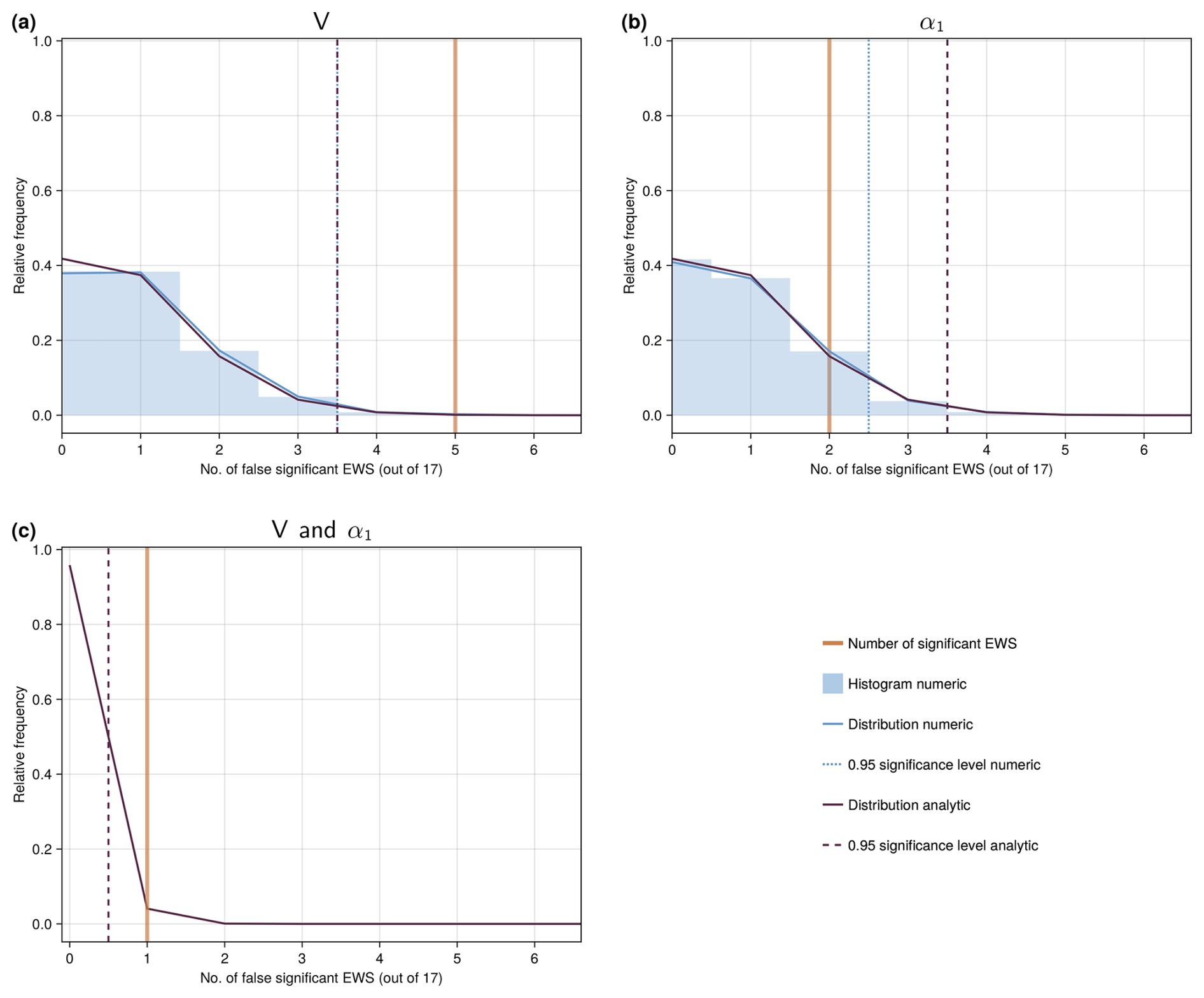
Figure 3 Null-model distributions for the number of significant EWS in V (a), α₁ (b), and both CSD-indicators simultaneously (c) for the NGRIP δ¹⁸O record with 5-year resolution.

The comparison of the analytical and numerical null-distributions primarily illustrates that our method of testing significance (Sect. 2.3) accurately represents the null-hypothesis and we don’t deem either of the two to be more meaningful than the other. In the following, we will primarily consider the binomial null-distribution for simplicity and easier comparison between the different records, since numerical distributions have only been calculated for the NGRIP record with 5 year resolution.

For a linear stochastic process not approaching a bifurcation, i.e. under the null hypothesis that there are no parameter changes in the underlying system, we would expect the estimates of increases in variability and correlation times to be independent. Hence, the number of spurious significant increases in two indicators, V and α₁, or ${\widehat{w}}^{\mathrm{2}}$ and ${\widehat{H}}^{\text{loc}}$ simultaneously, is expected to follow the binomial distribution B(n,p²). At 95 % confidence, one such simultaneous increase is statistically significant (Figs. 3c and A3c).

2.5 Overview of method modifications

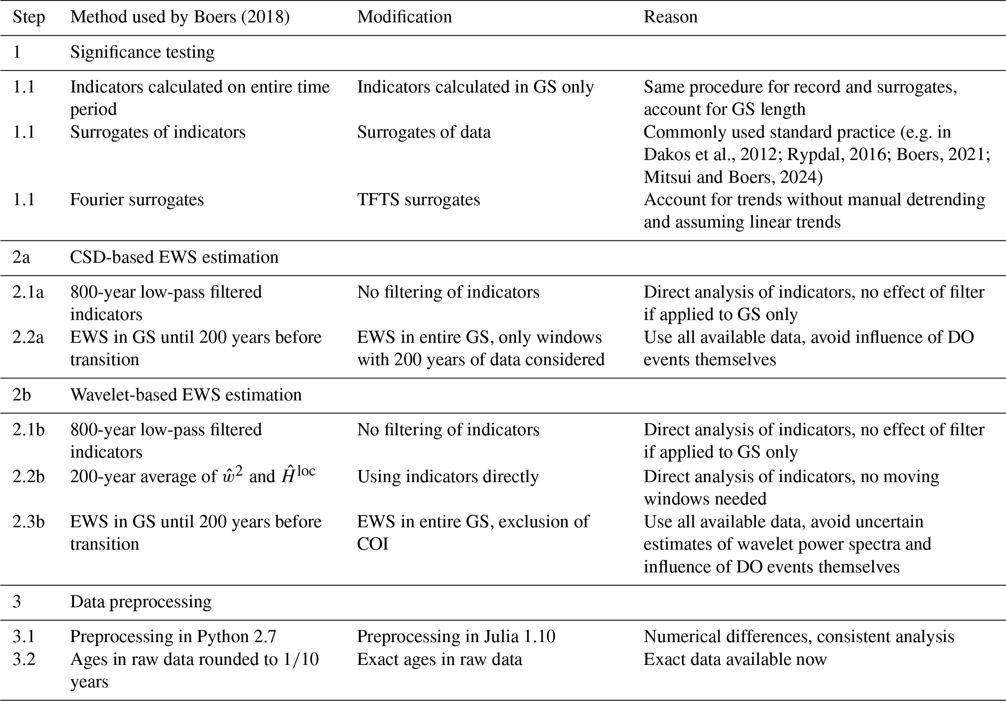
While our approach to data processing, EWS calculation and significance testing described above is based on the work by Boers (2018), some details differ from those applied there. Table 2 provides an overview of our modifications. We follow steps 1, 2a, and 3 for the CSD-based indicators, and steps 1, 2b, and 3 for their wavelet-based counterparts.

Boers (2018)Dakos et al., 2012; Rypdal, 2016; Boers, 2021; Mitsui and Boers, 2024

Table 2 Overview of method modifications compared to Boers (2018). Modifications to the methods used there are applied sequentially to the significance testing (Step 1), EWS estimation (Steps 2a and 2b for CSD- and wavelet-based indicators, respectively), and data processing (Step 3).

2.5.1 Significance testing

Rather than constructing surrogates by randomising the phases of the detrended indicator time series, we use the δ¹⁸O signal itself and keep the lowest 5 % of frequencies unchanged to account for possible trends in the data, without detrending manually. In order to construct surrogates of the data whilst still following the same procedure for surrogates and the δ¹⁸O record, we consider the indicator time series during GS individually. This differs from the approach by Boers (2018), where indicators were calculated over the entire time period and slices during GS were considered to search for EWS.

Since those modifications combined yield a different method of testing significance, they are not divided into sub-steps, as the changes in step 2 and 3 (see Table 2 and below), but are applied together. We change how significance is tested as a first step in the sequence of different modifications since we deem this to be the most important methodological change compared to Boers (2018).

2.5.2 EWS estimation

In contrast to Boers (2018), we do not apply a Chebyshev Type-I low-pass filter with cutoff at 800 years to extract millennial scale variability of the high-frequency indicator time series, but rather look for EWS in the indicator time series directly. We further note that such a filter does not yield an effect on the relatively short (35–8215 years; avg. 1588 years) time series during GS considered here.

Instead of searching for significant increases of variance and autocorrelation in the GS until 200 years before each transition using centered 200-year moving windows, we consider the entire GS but discard windows which contain less than 200 years of data.

To reap the advantage that using wavelet methods does not require moving time windows, we do not apply a 200-year average to ${\widehat{w}}^{\mathrm{2}}$ in Eq. (2). Similarly, we calculate the local Hurst exponent ${\widehat{H}}^{\text{loc}}$ for each time t directly without applying a moving 200-year average to $\left|W_t\right(s){|}^{\mathrm{2}}/s$ in Eq. (3) as done by Rypdal (2016) and Boers (2018). Furthermore, we don't restrict the search for wavelet-based EWS to the GS until 200 years prior to events, as in Boers (2018), to exclude potential influences of the transitions themselves. Instead, the entire GS is considered and any time points within the COI are discarded. Additionally, we consider the wavelet power spectra of the regularly sampled δ¹⁸O time series directly without normalisation.

2.5.3 Data preprocessing

Even though we follow the same steps in data preprocessing as Boers (2018), small differences between the δ¹⁸O records and thus the indicator time series arise. This is due to numerical differences and different implementations of e.g. the low- and high-pass filters between Python 2.7 used there and Julia 1.10 used here. Moreover, we analyse the publicly available NGRIP record, that differs slightly from the one used by Boers (2018), where the ages were rounded to one-tenth of a year.

3 Results

3.1 Early warning signals in the NGRIP record with 5-year resolution

For the δ¹⁸O record from NGRIP with 5 year time steps, we consider the CSD EWS V and α₁, as well as the restoring rate λ. We also look for significant increases of the scale-averaged wavelet coefficient ${\widehat{w}}^{\mathrm{2}}$ and the local Hurst exponent ${\widehat{H}}^{\text{loc}}$ preceding DO events. To be able to compare our results with those obtained by Boers (2018), we focus on the 10–50 year periodicity band. The resulting indicator time series are shown in Fig. 4.

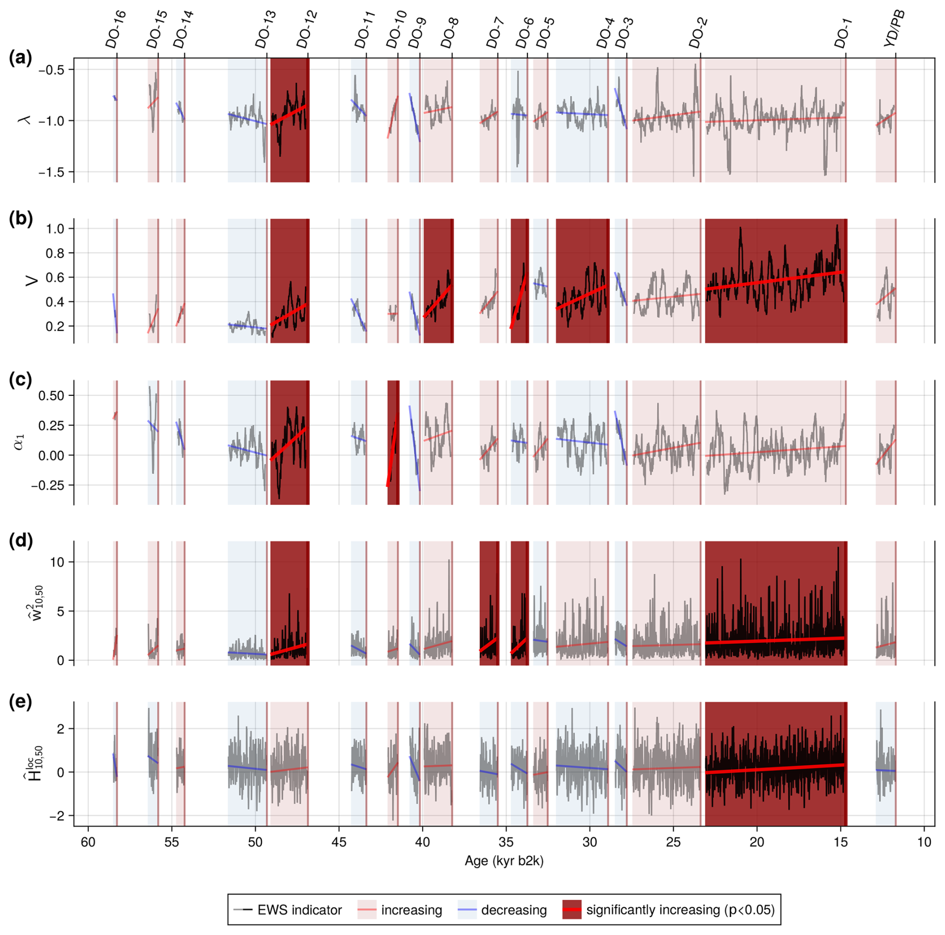
Figure 4 Early warning signals of the 5-year interpolated NGRIP δ¹⁸O record. (a) Time series of the restoring rate (black) of the 100-year high-pass filtered record during GS. (b–c) Same as (a) but for the variance and lag − 1 autocorrelation coefficient, respectively. (d–e) Time series of the the scale-averaged wavelet coefficient and local Hurst exponent confined to the 10–50 year periodicity band (black) during GS, respectively. DO events and the YD/PB transition are marked by the red vertical lines. Linear trends of the indicators are shown by red (blue) lines and the corresponding pale shading of the GS period if the trend is positive (negative). Significant linear increases are indicated by a dark red shading of the GS preceding transitions.

Considering the indicators of critical slowing down, we observe statistically significant increases prior to five DO events in V, whereas α₁ only shows significant increases preceding two events, and λ only displays one significant EWS. Similarly, we find four significant increases in ${\widehat{w}}^{\mathrm{2}}$, but only one in ${\widehat{H}}^{\text{loc}}$.

According to the binomial null-distributions for spuriously appearing early warning signals (Figs. 3, A3 and Sect. 2.4), the numbers of significant increases in V and ${\widehat{w}}^{\mathrm{2}}$ are statistically significant at 95 % confidence. This is also the case for the simultaneous warning from the CSD-indicators for DO-12, as well as the simultaneous significant increase in the wavelet-based indicators preceding DO-1. Though, observing two significant EWS in α₁ and one in the restoring rate, as well as the local Hurst exponent is not significant.

We observe that three of the four events (DO-1, 6, and 12) displaying significant EWS in ${\widehat{w}}^{\mathrm{2}}$ also show significant increases in V, whereas significant EWS in α₁ and ${\widehat{H}}^{\text{loc}}$ do not coincide.

Regarding individual DO events, we find that DO-12 is preceded by significant EWS in all indicators, except ${\widehat{H}}^{\text{loc}}$. Both wavelet-based indicators, as well as the variance show a warning prior to DO-1 and DO-6 is preceded by significant increases in the variability indicators V and ${\widehat{w}}^{\mathrm{2}}$.

Even though the numbers of significant EWS in the high-frequency variability of the NGRIP δ¹⁸O record could potentially be seen as evidence for a destabilisation of the system, those for the correlation times do not indicate a consistent widening of the basin of attraction associated with mechanisms operating on decadal time scales, across the series of DO events.

Furthermore, we note that while both CSD- and wavelet-based indicators show a statistically significant simultaneous significant increase in variability and correlation times, these do not occur for the same transitions (DO-12 for the CSD indicators (Fig. 4a, b, c), and DO-1 for the wavelet-based ones (Fig. 4d, e), respectively).

3.1.1 The restoring rate λ

Since EWS in the wavelet-based and commonly used CSD indicators V and α₁ might stem from external contributions not related to critical slowing down, we also estimate the restoring rate λ for this record (Fig. 4a), which is more robust towards changes of the statistical properties of noise acting on the record (Boers, 2021). Fig. 5 shows the Pearson correlation coefficients between λ and the other EWS indicators during GS.

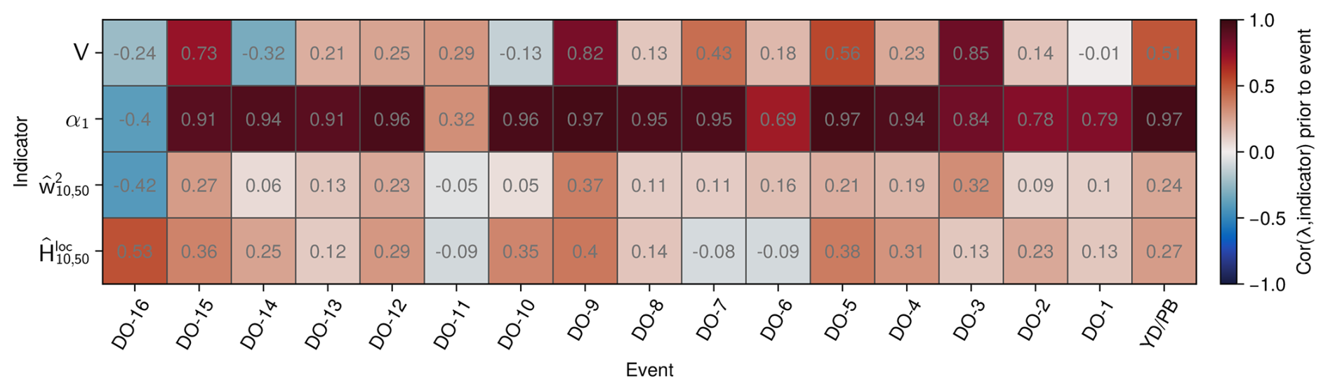
Figure 5 Correlation between early warning indicators and the restoring rate of the 5-year interpolated NGRIP δ¹⁸O record. Colours and grey text indicate values of the Pearson correlation coefficient between the restoring rate λ and the variance, lag − 1 autocorrelation, scale-averaged wavelet coefficient, and local Hurst exponent, respectively (top to bottom) during GS prior to DO events and the YD/PB transition (left to right), as presented in Fig. 4.

We find high positive correlations (≥ 0.78) prior to most DO events between λ and the lag − 1 autocorrelation coefficient α₁, as it can also be seen in the respective time series in Fig. 4a and c. We also observe high correlation values (= 0.96) prior to DO-12 and 10, for which α₁ displays EWS. Thus, it seems likely that the autocorrelation estimates α₁ do not capture changes in the autocorrelation structure of noise acting on the record and that the EWS, at least prior to DO-12, where λ significantly increases as well, is indeed an indicator of CSD.

For the variance V, only three GS (prior to DO-15, 9, and 3) show high positive (≥ 0.73) correlation values. Nevertheless, during GS where the variance increases significantly (DO-12, 8, 6, 4, and 1), the correlation coefficient remains comparably low (≤ 0.25). The two wavelet-based indicators only correlate weakly with λ (≤ 0.38 and 0.53 for ${\widehat{w}}^{\mathrm{2}}$ and ${\widehat{H}}^{\text{loc}}$, respectively). While these correlation results could indicate that the variance and wavelet-based indicators might not directly capture changes in stability during most GS, we also note that the theoretical framework behind these early warning indicators, including λ, is based on one-dimensional conceptual models, whereas the processes influencing the δ¹⁸O record are far more complex. Moreover, the Pearson correlation coefficient only measures linear correlations. Nevertheless, the simultaneous warning prior to DO-12 by λ, V, and ${\widehat{w}}^{\mathrm{2}}$ suggests that the variability indicators capture a destabilisation in this time period.

3.1.2 Method modifications

When searching for EWS, many methodological choices have to be made. Here, we systematically test the robustness of early warning signals to a variety of such choices. To do so, we analyse the methods of Boers (2018) and sequentially evaluate modifications in the significance testing, EWS calculation, and data preprocessing for the high-frequency variability of the NGRIP record, following steps 1, 2a, and 3 in Table 2 for the CSD indicators V and α₁, and steps 1, 2b, and 3 for the wavelet-based indicators ${\widehat{w}}_{\mathrm{10},\mathrm{50}}^{\mathrm{2}}$ and ${\widehat{H}}_{\mathrm{10},\mathrm{50}}^{\text{loc}}$, which are further described in Sect. 2.5.

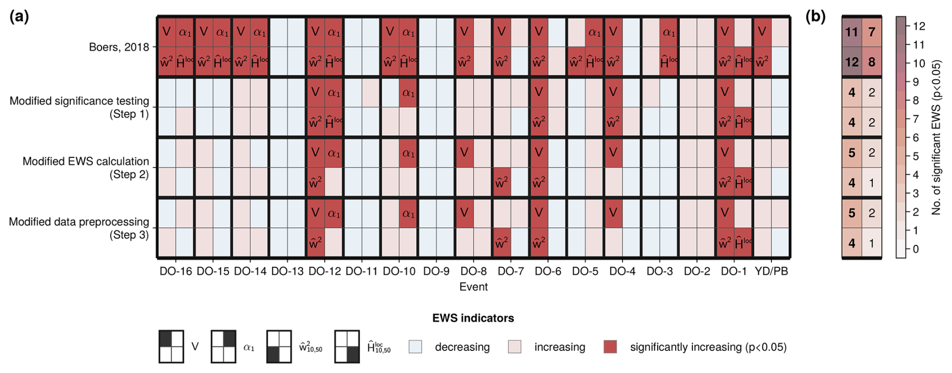
Figure 6 Early warning signals of the 5-year interpolated NGRIP δ¹⁸O record with sequential method modifications. (a) Linear trends of the indicators (variance, lag − 1 autocorrelation coefficient, scale-averaged wavelet coefficient and local Hurst exponent) during GS prior to DO events and the YD/PB transition (left to right) calculated using the methods described by Boers (2018), with sequential modifications to the significant testing, estimator calculation and data processing (top to bottom). Positive (negative) trends are marked in red (blue). Significant increases are displayed in dark red and marked with the indicator name. (b) Number of statistically significant EWS in the different indicators and modification steps. Bold values indicate that the number of significant EWS is statistically significant at 95 % confidence.

The resulting influences of these sequentially applied modifications on the EWS indicators can be seen in Fig. 6. The corresponding time series are shown in Figs. S7 and S9 for the CSD and wavelet-based indicators, respectively. Figures S8 and S10 provide a more detailed synopsis following all sub-steps.

While attempting to recreate the results of Boers (2018), we find significant EWS for 11 out of 17 transitions in the variance V, seven in the autocorrelation α₁, and five for both CSD indicators simultaneously. This differs from the results of Boers (2018) which show an additional event with a significant increase in variance (n_V=12, $n_{{\mathit{\alpha }}_{\mathrm{1}}}=\mathrm{7}$, and n_both=6). The additional EWS in V stems from an erroneous calculation there, where the time series of the scale-averaged wavelet coefficient ${\widehat{w}}^{\mathrm{2}}$ was considered instead of the variance V. For the wavelet-based indicators, we find the same significant EWS, i.e. 12 significant increases in ${\widehat{w}}^{\mathrm{2}}$, 8 in ${\widehat{H}}^{\text{loc}}$, and 7 in both indicators simultaneously.

As a first robustness test, we modify how surrogates are obtained for significance testing and construct surrogates of the data during GS prior to transitions, instead of the indicator time series. This decreases the number of significant EWS from 11 to 4 in V, and from 7 to 2 in α₁. Only one event (DO-12) shows a simultaneous significant increase in both V and α₁. As for the CSD-based indicators, our modifications in significance testing result in fewer significant wavelet-based EWS in both indicators with $n_{{\widehat{w}}^{\mathrm{2}}}=\mathrm{4}$ (for DO-1, 4, 6, and 12), $n_{{\widehat{H}}^{\text{loc}}}=\mathrm{2}$, and n_both=2 (for DO-1 and 12). We note that the resulting indicator time series differ and appear less smooth because applying a 800-year low-pass filter, as done by Boers (2018) doesn't yield the same effect when applied to the GS rather than the entire time period (see Figs. S7a–d and S9a–d).

Next, when modifying how V and α₁ are calculated, the previously significant EWS remain. For the variance, one event (DO-8) that shows a significant increase with the initial significance testing, but not the modified one, now displays early warning. As in the previous step, only one event is preceded by precursors in both variance in autocorrelation, i.e. n_V=5 (prior to DO-1, 4, 6, 8, and 12), $n_{{\mathit{\alpha }}_{\mathrm{1}}}=\mathrm{2}$ (prior to DO-10 and 12), and n_both=1 (prior to DO-12). Modifications to the EWS estimation lead to the same number of significant increases in the wavelet coefficient as in the previous step ($n_{{\widehat{w}}^{\mathrm{2}}}=\mathrm{4}$ preceding DO-1, 6, 7, and 12). While two of them (for DO-1 and 6) were significant before, one increase lost its significance, and another one (prior to DO-7) became significant again. For ${\widehat{H}}^{\text{loc}}$, one increase loses significance, resulting in only one event (DO-1) with a significant EWS in the local Hurst exponent, as well as both wavelet-based stability estimators simultaneously. Finally, we change how the δ¹⁸O record is preprocessed and obtain the indicator time series displayed in Fig. 4b–e. These modifications do not yield any further changes to any of the early warning signals of the NGRIP record.

The modifications shown here are applied in sequence. Nevertheless, we find that step 1 (changes to the significance testing) yields the biggest decrease in the number of significant EWS, compared to steps 2 (EWS calculation) and 3 (data preprocessing), also when applied individually.

3.2 Early warning signals in the NGRIP record with irregular temporal resolution

For the raw NGRIP δ¹⁸O record with variable time steps, we make use of the adapted methods introduced by Mudelsee (2002) and Lenoir and Crucifix (2018a) as described in Sect. 2.2. A technical difference between this approach and the one we use for the regularly sampled records is the choice of the Morlet wavelet as the mother wavelet instead of the Paul wavelet for the estimation of ${\widehat{w}}^{\mathrm{2}}$ and ${\widehat{H}}^{\text{loc}}$. Thus, to compare wavelet-based EWS between the raw and interpolated data, the analysis of the interpolated time series is repeated using the Morlet wave basis here. Fig. 7 shows the resulting early warning signals. The corresponding indicator time series are displayed in Figs. S11 and S12.

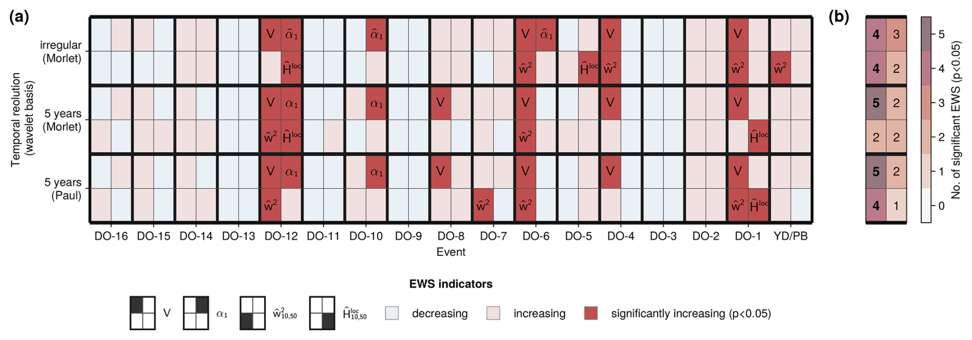
Figure 7 Early warning signals of the raw, irregularly sampled and 5-year interpolated NGRIP δ¹⁸O record. (a) Linear trends of the indicators (variance, lag − 1 autocorrelation coefficient, scale-averaged wavelet coefficient, and local Hurst exponent) during GS prior to DO events and the YD/PB transition (left to right) of the irregularly sampled NGRIP record using the Morlet wavelet basis for the calculation of the wavelet-based indicators ${\widehat{w}}_{\mathrm{10},\mathrm{50}}^{\mathrm{2}}$ and ${\widehat{H}}_{\mathrm{10},\mathrm{50}}^{\text{loc}}$ (top), the 5-year interpolated record using Morlet (middle), and the 5-year interpolated record using the Paul wavelet basis (bottom). Positive (negative) trends are marked in red (blue). Significant increases are displayed in dark red and marked with the indicator name. (b) Number of statistically significant EWS in the different indicators, for regular and irregular resolutions, and different wavelet bases. Bold values indicate that the number of significant EWS is statistically significant at 95 % confidence.

Regarding variance and autocorrelation of the raw, irregularly sampled record, we we find four significant EWS in V (prior to DO-1, 4, 6, and 12), and three in ${\widehat{\mathit{\alpha }}}_{\mathrm{1}}$ (for DO-6, 10, and 12), where two events (DO-6 and 12) show synchronous significant increases in both indicators. Considering the binomial null distributions for false positives, the observed number of significant increases in the variance, and both CSD-indicators simultaneously is statistically significant at 95 % confidence, whereas this is not the case for the autocorrelation. While all significant variance increases in the raw time series are also found in the interpolated record with even time sampling, there is one event (DO-8) that is not preceded by an early warning here. Two of the three GS (prior to DO-10 and 12) displaying significant ${\widehat{\mathit{\alpha }}}_{\mathrm{1}}$ increases in the raw record, also show significant increases in α₁ of their regularly sampled counterparts. In both cases, DO-12 is preceded by significant EWS in both CSD-estimators, and analysis of the irregularly sampled raw record reveals another simultaneous warning for DO-6.

When searching for wavelet-based EWS in the raw δ¹⁸O NGRIP record, we find four significant EWS in the scale-averaged wavelet coefficient ${\widehat{w}}^{\mathrm{2}}$ (for the YD/PB transition, DO-1, 4, and 6) and two in the local Hurst exponent ${\widehat{H}}^{\text{loc}}$ (for DO-12 and 5). None of the 17 events show simultaneous increases in both indicators in the 10–50 year periodicity band. When applying the Morlet wave basis, we observe two EWS in ${\widehat{w}}^{\mathrm{2}}$ (prior to DO-6 and 12), and ${\widehat{H}}^{\text{loc}}$ (prior to DO-1 and 12) in the interpolated time series. Comparing the regularly and irregularly sampled versions of the NGRIP record using this wave basis, we see that DO-12 is preceded by significant increases in ${\widehat{H}}^{\text{loc}}$ for both of them. Further, they share one common significant increase in ${\widehat{w}}^{\mathrm{2}}$ prior to DO-6. The raw record displays a significant number of significant increases in the scale-averaged wavelet coefficient at 95 % confidence. The number of significant EWS in the local Hurst exponent might be spurious for either record. Nonetheless, the occurrence of a simultaneous significant increase in both indicators prior to DO-12 in the interpolated record is statistically significant.

While using the Morlet mother wavelet yields two significant increases less in ${\widehat{w}}^{\mathrm{2}}$ compared to their estimation using the Paul wavelet, we find two additional significant EWS in ${\widehat{H}}^{\text{loc}}$. Either choice of wavelet function yields one event with a simultaneous increase in both indicators. Nevertheless, these occur for different events: DO-1 using Paul and DO-12 using Morlet.

3.3 Early warning signals across ice core records

To be able to compare wavelet-based EWS between the various ice core records with different temporal resolutions, ranging from 5 to 20 years, we focus on ${\widehat{w}}^{\mathrm{2}}$ and ${\widehat{H}}^{\text{loc}}$ in the 20–60 year frequency band instead of the 10–50 year one considered before. These EWS, as well as the ones in variance and autocorrelation for the various δ¹⁸O records from Greenland ice cores are depicted in Fig. 8. Figures S13 and S14 show the CSD- and wavelet-based indicator time series, respectively.

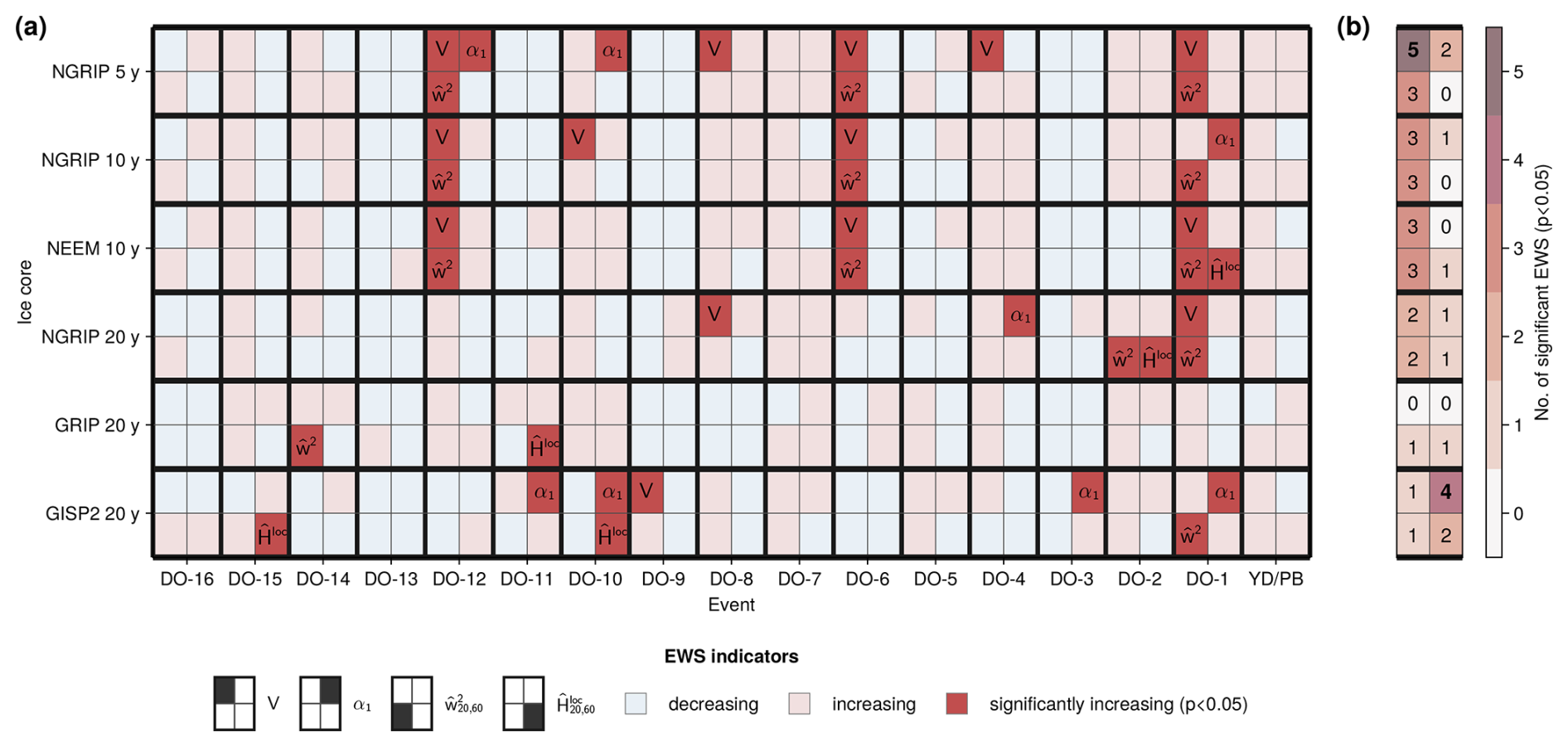
Figure 8 Early warning signals of various Greenland δ¹⁸O records. (a) Linear trends of the indicators (variance, lag − 1 autocorrelation coefficient, scale-averaged wavelet coefficient, and local Hurst exponent) during GS prior to DO events and the YD/PB transition (left to right) for the 5-year NGRIP record, 10-year NGRIP record, 10-year NEEM record, 20-year NGRIP record, 20-year GRIP record, and 20-year GISP2 record (top to bottom). Positive (negative) trends are marked in red (blue). Significant increases are displayed in dark red and marked with the indicator name. (b) Number of statistically significant EWS in the different indicators and ice core records. Bold values indicate that the number of significant EWS is statistically significant at 95 % confidence.

Only NGRIP with 5-year sampling steps shows a significant EWS for V and α₁ simultaneously (DO-12). Two of the records, NEEM in 10- and NGRIP in 20-year resolution, show a simultaneous warning in ${\widehat{w}}^{\mathrm{2}}$ and ${\widehat{H}}^{\text{loc}}$ (for DO-1 and DO-2, respectively). These are statistically significant results at the 95 % confidence level. Nevertheless, we note that DO-2 is not preceded by any significant EWS in any other record considered here.

The number of significant variance increases ranges from zero (GRIP, 20-year resolution) to five (NGRIP, 5-year resolution). For the autocorrelation, this number ranges from zero to four, but in this case NEEM in 10-year resolution and GRIP in 20-year resolution display the fewest, whereas GISP2 in 20-year resolution shows the most EWS. Considering ${\widehat{w}}^{\mathrm{2}}$, the number of significant EWS ranges from one (GRIP and GISP2 with 20-year resolution) to three (NGRIP with 5-year sampling and both 10-year resolution records) and for ${\widehat{H}}^{\text{loc}}$ from zero (NGRIP with 5- and 10-year resolution) to two (GISP2, 20-year resolution). The numbers of significant increases in the variance are only statistically significant for the NGRIP record with 5-year resolution. For the autocorrelation, only GISP2 in 20-year resolution displays a significant number of significant EWS at 95 % confidence, whereas these numbers are not significant for the scale-averaged wavelet coefficient or the local Hurst exponent.

None of the 17 events is preceded by a common significant EWS in any indicator across all records. Nevertheless, DO-1 is anticipated by significantly increasing ${\widehat{w}}^{\mathrm{2}}$ in most records (except for GRIP). For this event, we also find three common significant increases in variance across the different records for the signal from NGRIP in 5- and 20-year resolutions, as well as NEEM. It is also preceded by a common increase in the autocorrelation in the 10-year NGRIP record and the 20-year GISP2 record. Furthermore, DO-12 and DO-6 display significant increases in both V and ${\widehat{w}}^{\mathrm{2}}$ for all the high-resolution records (NGRIP 5- & 10-year, NEEM 10-year sampling).

Regarding the EWS in the NGRIP record across different temporal resolutions, we note that the 5-year and 10-year resolution signals share two common events (DO-12 and DO-6) with preceding EWS in V. The 5- and 20-year sampled records share the two significant variance increases present for the latter (DO-1 and DO-8). We find a common significant increase in the scale-averaged wavelet coefficient for DO-1 across all resolutions, and DO-6 and DO-12 are preceded by significant increases for 5- and 10-year sampling steps. Further, neither the autocorrelation nor the local Hurst exponent show a common significant increase across the different resolutions of the NGRIP record.

Comparing records with the same temporal resolution, we find two common significant EWS in V (DO-12 and DO-6) for NGRIP and NEEM, sampled every 10 years, and none for the time series with 20-year time steps. We further see that all three significant increases in ${\widehat{w}}^{\mathrm{2}}$ prior to DO-1, 6, and 12 are common across the 10-year resolution records. DO-1 also has a common significant EWS in the scale-averaged wavelet coefficient for NGRIP and GISP2, but not across all 20-year records.

While we seem to find more significant increases in V and ${\widehat{w}}^{\mathrm{2}}$ for the high-resolution records, there is no such apparent trend for α₁ or ${\widehat{H}}^{\text{loc}}$.

For a comparison of common CSD EWS across records, see also Fig. S15. An overview of wavelet-based EWS in the different frequency bands (s₁,s₂) relevant for all of the considered records can be found in Fig. A4. There, we see that there is no such band with a common significant indicator increase in all of the records, but common significant increases of ${\widehat{w}}^{\mathrm{2}}$ for DO-1 are found in all records but GISP2 in three frequency bands. Furthermore, DO-1, 6, and 12 are preceded by common significant EWS of the higher resolution records for a range of high-frequency scale ranges. Regarding the local Hurst exponent, only few common significant EWS are found across all considered scales and only for the different versions of the NGRIP record. We only observe one common significant increase in both wavelet-based indicators simultaneously prior to DO-1 for NGRIP in 5- and 10-year resolution. Other simultaneous EWS of both indicators are found for different scale ranges prior to DO-1, 2 and 6 in NGRIP and NEEM (see Figs. S16 and S17).

The numbers of significant increases of ${\widehat{w}}^{\mathrm{2}}$ and ${\widehat{H}}^{\text{loc}}$ for frequency bands relevant for the individual records are depicted in Fig. A5. It reveals that the numbers of significant increases in ${\widehat{w}}^{\mathrm{2}}$ are only statistically significant at 95 % for the NGRIP record with high temporal resolutions ≤10 years for few scale bands. Nevertheless, there are such bands for NGRIP in all considered resolutions and NEEM where simultaneous increases in ${\widehat{w}}^{\mathrm{2}}$ and ${\widehat{H}}^{\text{loc}}$ occur. Out of all the cases considered, only the δ¹⁸O record from GRIP displays a significant number of significant increases in ${\widehat{H}}^{\text{loc}}$ for one scale band. Further synopses of the wavelet-based indicators across the various records and scale ranges are depicted in Figs. S18 and S19.

3.4 Summary of results

Throughout our analysis we found rather low but varying numbers of significant EWS across different indicators and δ¹⁸O records. These appear to be statistically significant at 95 % confidence primarily for NGRIP with irregular and 5-year temporal resolution and the indicators of high-frequency variability V and ${\widehat{w}}^{\mathrm{2}}$. Considering the wavelet-based estimators, it appears that the choice of wavelet basis plays a critical role in whether a significant amount of EWS in ${\widehat{w}}^{\mathrm{2}}$ is observed.

An overview of the number of significant EWS, as well as their statistical significance, across the different ice core records and a selection of indicators is shown in Fig. 9.

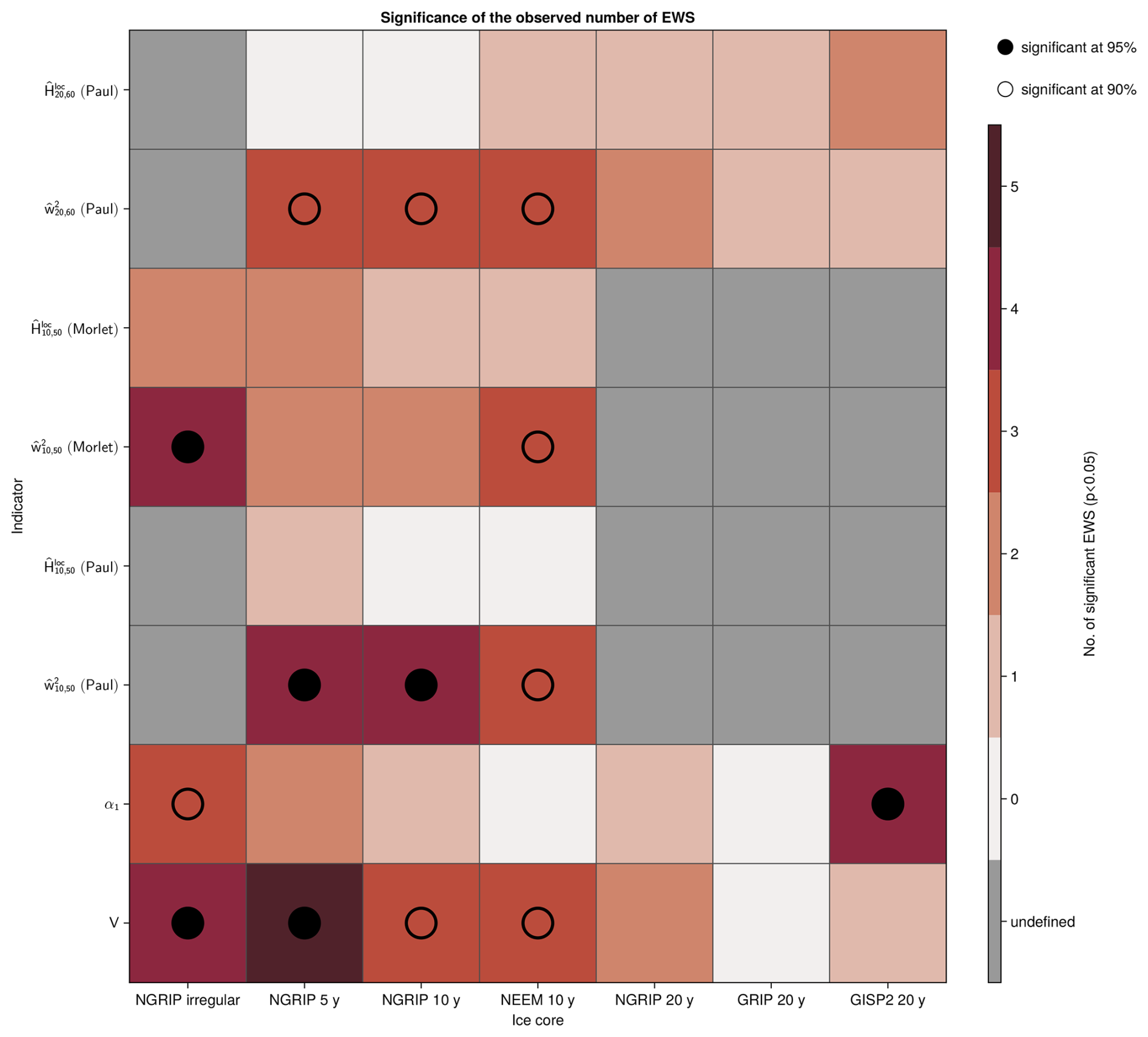
Figure 9 Numbers of significant EWS and their statistical significance at 90 % and 95 % across various δ¹⁸O records from Greenland ice cores and a selection of indicators. Ice core records are denoted by their location and temporal resolution. The wavelet-based indicators ${\widehat{w}}_{s_{\mathrm{1}},s_{\mathrm{2}}}^{\mathrm{2}}$ and ${\widehat{H}}_{s_{\mathrm{1}},s_{\mathrm{2}}}^{\text{loc}}$ are specified by the choice of wavelet basis, and the considered scale ranges between s₁ and s₂ years.

3.4.1 NGRIP

For the NGRIP record interpolated to 5-year time steps, we find fewer significant EWS compared to Boers (2018), when significance testing is altered. Further changes in EWS indicator calculation and data preprocessing were found to have a minor influence. Nonetheless, our results also indicate a lower number of spurious early warnings in all the estimators considered. We observed a strong agreement between the binomial and numerically constructed null-distributions of false positives. Hence, we argue that our surrogate model, used to determine whether an EWS is significant, better represents the null hypothesis of DO events occurring due to random fluctuations.

The numbers of significant increases for this record are statistically significant at 95 % confidence for the variability estimators V and ${\widehat{w}}_{\mathrm{10},\mathrm{50}}^{\mathrm{2}}$ using the Paul wavelet function, as well as simultaneous occurrences of CSD- and wavelet-based EWS, respectively. However, we note that these simultaneous EWS do not occur before the same transitions for the CSD- and wavelet-based indicators (DO-12 and 1, respectively) and not all variability indicator increases are preceding the same DO events.

The choice of wavelet basis function for the calculation of the wavelet-based indicators was found to be critical for the detection of significant EWS, where increases prior to DO-1, 6 and 12 appeared to be less sensitive.

Applying specialised approaches for irregularly sampled time series to the raw NGRIP record yields similar results as for the regularly-sampled one. The number of significant increases is statistically significant at 95 % confidence for both variability indicators (V and ${\widehat{w}}_{\mathrm{10},\mathrm{50}}^{\mathrm{2}}$), and the simultaneous warning from both CSD EWS.

3.4.2 Comparison of ice core records

Most transitions do not show consistent EWS across various δ¹⁸O records with regular time steps from different Greenland ice cores, with the notable exception of DO-1, and to a lesser degree DO-6 and 12, which agree in EWS of the variability indicators in the high-resolution records from NGRIP and NEEM. Nevertheless, only the NGRIP record sampled every 5 years displays a significant number of significant EWS in the variance, and both CSD indicators simultaneously, while this number is not significant for ${\widehat{w}}_{\mathrm{20},\mathrm{60}}^{\mathrm{2}}$ in any of the records.

We find fewer EWS and less agreement for GRIP and GISP2. For the estimators of correlation times, we only find a statistically significant number of EWS in α₁ in the GISP2 record, that otherwise doesn't display a significant number of significant indicator increases. Only few significant increases in ${\widehat{H}}_{\mathrm{20},\mathrm{60}}^{\text{loc}}$ are seen, and the observed numbers are not statistically significant at 95 % confidence for any of the records.

4 Discussion and conclusions

4.1 Differences between the ice core records

While the δ¹⁸O records from the four different ice core sites all show the same synchronous behaviour during GS/GI transitions (Guillevic et al., 2013; Seierstad et al., 2014) (see Fig. 2), they differ in some aspects besides their resolution.

GRIP and GISP2 are located approx. 28 km apart from each other on the summit of the Greenland ice sheet (Guillevic et al., 2013), whereas NGRIP was drilled on the ice divide, approx. 325 km north-west of GRIP (North Greenland Ice Core Project members et al., 2004). NEEM lies ca. 350 km further north-west along this divide (Erhardt et al., 2022). The locations of these ice core sites are depicted in Fig. 1.

It has been shown before that δ¹⁸O values are systematically between 1 ‰ and 3 ‰ lower in NGRIP compared to GRIP and GISP2 throughout the last glacial period (North Greenland Ice Core Project members et al., 2004; Guillevic et al., 2013; Seierstad et al., 2014). We also note that these values are comparable between NGRIP and NEEM (Guillevic et al., 2013), as well as GRIP and GISP2 (Seierstad et al., 2014), respectively. For DO-8 and 10, Guillevic et al. (2013) found that the difference in the water isotopic ratio δ¹⁸O between GS and GI decreases from North Western Greenland to its summit (i.e. from NEEM, over NGRIP towards GRIP and GISP2). While these discrepancies between the signals do not necessarily influence the EWS considered here, they are remarkable and indicate important regional variations, given the geographical proximity of the ice core sites (North Greenland Ice Core Project members et al., 2004).

Oxygen isotope ratios δ¹⁸O are often used as temperature proxies of the past (Dansgaard, 1964), but they are also influenced by complex effects from the mixing of air masses (Charles et al., 1994). Important factors are the distance and temperature gradient between the ice core and its source region of precipitation (Jouzel et al., 2000; Steen-Larsen et al., 2013), as well as seasonality biases of the received precipitation (Krinner et al., 1997; Werner et al., 2000; Langen and Vinther, 2009; Seierstad et al., 2014). Indeed, for DO-8, 9 and 10, the temporal sensitivity of δ¹⁸O to temperature was found to vary from 0.34 ‰ °C⁻¹ to 0.68 ‰ °C⁻¹, where it decreases with site elevation, i.e. from NEEM over NGRIP to the summit sites GRIP and GISP2 (Guillevic et al., 2013). The interpretation of δ¹⁸O as “paleo thermometer” has further been challenged by a recent modelling study (Buizert et al., 2024) using a state-of-the art isotope-enabled climate model. Their results suggest that δ¹⁸O during DO events may not be controlled by temperatures at the ice core sites. Instead, winter sea ice variations in the North Atlantic were found to be the dominant control.

Possible reasons for the spatial inhomogeneities between the records include changes in moisture origin and transport paths, precipitation seasonality, meso-scale atmospheric dynamics and local processes (Guillevic et al., 2013; Steen-Larsen et al., 2013; Seierstad et al., 2014; Capron et al., 2021). Differences between the records on shorter (sub-millennial) time scales are thought to have been driven by rapid sea ice and/or sea surface temperature changes in the North Atlantic, which were found to have a stronger influence on the δ¹⁸O variability in North-West Greenland (at NGRIP and NEEM) than on the summit (at GRIP and GISP2) (Guillevic et al., 2013; Seierstad et al., 2014). Multiple previous studies suggest that DO events in Greenland were triggered by a rapid sea ice retreat in the North Atlantic (Broecker et al., 1985; Ganopolski and Rahmstorf, 2001; Gildor and Tziperman, 2003; Li et al., 2010; Dokken et al., 2013; Petersen et al., 2013; Zhang et al., 2014; Hoff et al., 2016; Vettoretti and Peltier, 2016; Boers et al., 2018; Vettoretti and Peltier, 2018; Li and Born, 2019; Riechers et al., 2023a; Buizert et al., 2024). The influences of those changes on δ¹⁸O values may therefore be more pronounced in the NGRIP and NEEM records, potentially contributing to the more frequent and consistent presence of EWS in these records.

Another factor that might play into the similarity of results between the two records from the Greenland divide, NGRIP and NEEM, could be that the NEEM ice core is located downstream of NGRIP (Dahl-Jensen et al., 2013; Montagnat et al., 2014). It has been shown before that the current NEEM site was located at a higher altitude and further upstream, closer to NGRIP than it is today (Dahl-Jensen et al., 2013), whereas past NGRIP deposition sites were situated fairly close to its present-day location (Nixdorf and Göktas, 2001) due to a constant horizontal velocity along the ridge around NGRIP (Dahl-Jensen et al., 2002).

Another inconsistency across the sites are snow accumulation rates. GRIP and GISP2 are believed to have similar accumulation histories, with higher rates than at NGRIP and NEEM (Guillevic et al., 2013; Seierstad et al., 2014). A previous study (Münch et al., 2016) on Antarctic ice cores indicates that in δ¹⁸O records from locations with low snow accumulation, the highest frequencies may predominantly be influenced by disturbances occurring after deposition. While the sites studied there generally display substantially lower accumulation than the Greenland sites, it is important to note that Greenland accumulation rates decrease to comparable low values during GS (Guillevic et al., 2013; Seierstad et al., 2014; Münch et al., 2016). Hence, we cannot rule out that the observed EWS are influenced by such intrinsic noise.

The reduced number of significant EWS for DO-1 in GRIP and GISP2, compared to NGRIP and NEEM might be explained by important uncertainties in the time scale transfer from NGRIP during long stadials, such as GS-2.1 preceding DO-1 (Seierstad et al., 2014). Regardless, even larger uncertainties were estimated for NEEM during the same period (Rasmussen et al., 2013).

Possible reasons for the differences in results for the GISP2 record might be related to the missing values in the δ¹⁸O time series (see Sect. 2.1.1 for details). Moreover, parts of this record had to be corrected for alterations of δ¹⁸O by the way some of the ice core samples have been stored (Stuiver et al., 1995). Nonetheless, these corrections were later found to have a minor influence on parts of the record (Stuiver and Grootes, 2000). Those inconsistencies might further be related to the fact that δ¹⁸O from NGRIP, NEEM, and GRIP has been measured at the University of Copenhagen (Johnsen et al., 1997; North Greenland Ice Core Project members et al., 2004; Gkinis et al., 2014, 2021), whereas the GISP2 has been analysed at the University of Washington (Stuiver and Grootes, 2000), because the higher-order statistics that are computed to obtain the different EWS indicators can be influenced by the processing of the raw ice core data to derive the final time series. This can lead to biases and, hence, to a masking of an underlying signal of critical slowing down and associated EWS. The degree to which this occurs depends on the exact preprocessing conducted for each core, and therefore we cannot expect to obtain the same EWS for different ice cores, processed differently in different labs. We further argue that this does not yield a limitation of the usefulness of EWS indicators, but rather reflects the impact of the underlying uncertainties.

The aim of this discussion is not to give a comprehensive overview of possible drivers of differences in δ¹⁸O records from Greenland ice cores. Instead, it serves to illustrate that there is a diverse range of factors, other than a common high-frequency climate signal, that could have major influences on the results presented here.

4.2 Implications of results

In comparison to the results by Boers (2018), our analysis reveals fewer significant EWS for individual DO events in the high-frequency variability of the high resolution NGRIP record. Only few events, notably DO-1, 6, and 12, are preceded by consistent significant increases across the different variability indicators and the various δ¹⁸O records studied here. While multiple previous studies also found significant EWS for DO-1 (Rypdal, 2016; Boers, 2018; Myrvoll-Nilsen et al., 2025) and DO-12 (Rypdal, 2016; Boers, 2018) only the results from Boers (2018) indicate a destabilisation prior to DO-6.

Since the δ¹⁸O records considered differ in many aspects, such as ice core location, processing and temporal resolution, observing significant EWS in some, but not all records does not necessarily imply a false positive. It could simply be that an underlying true EWS is masked in an individual record, with preprocessing steps affecting the different EWS indicators in different ways.

We found a statistically significant amount of significant early warnings in the CSD- and wavelet-based indicators of high-frequency variability, especially for the NGRIP δ¹⁸O record with high temporal resolution. However, due to lack of consistent accompanying EWS in correlation times, we find only weak evidence for a destabilising state prior to these or any of the DO transitions, which would be expected if they were bifurcation-induced.

Significant numbers of significant EWS in other δ¹⁸O records were only detected for α₁ in GISP2 and ${\widehat{w}}^{\mathrm{2}}$ in two scale bands in NEEM. One reason for the fewer observed and less consistent significant EWS in V and ${\widehat{w}}^{\mathrm{2}}$ for NGRIP, GRIP and GISP2 sampled every 20 years might be that their resolution is too coarse to study imprints of processes on (sub-)centennial time scales. We further note that the differences between the NGRIP record in different resolutions may be caused by sampling effects and/or a result of spurious EWS.

We do not find clear support for the hypothesis that any of the analysed transitions are caused by a bifurcation in a dynamical subsystem operating at decadal time scales, as proposed by Rypdal (2016) and previously confirmed by Boers (2018). It is important to note that our findings cannot be used to reject such a hypothesis either, and that the observed precursor signals do not directly yield an indication on which tipping mechanisms might be most relevant for DO events.

The indicators used in this study are based on relatively simple low-dimensional dynamical systems characterised by specific bifurcation and noise structures (Scheffer et al., 2009; Ditlevsen and Johnsen, 2010; Kuehn, 2011). However, they may not produce equivalent results when applied to observational data from more complex systems, such as the Earth's climate, which features more intricate bifurcation structures, varied noise processes, and many interacting time scales. This suggests the need for a more cautious approach, one that is specifically tailored to the unique properties of the underlying system – assuming these properties are well-understood. Consequently, gaining a deeper insight into the processes driving DO cycles becomes essential. Recent advancements in EWS methods have expanded to address various noise processes (Kuehn et al., 2022; Morr and Boers, 2024) and introduced new methodologies (Clarke et al., 2023). However, there remains a significant need for further research into the applicability of EWS.

Despite the simplicity of the EWS used in our analysis, we faced numerous decisions regarding parameters, significance tests, and computational details. These choices can substantially influence results, as evidenced by our comparisons with the findings of Boers (2018) (Fig. 6) and our adaptations for analysing irregularly sampled time series (Fig. 7). We further remark that our analysis does not aim to reveal a “best way” on how to calculate early warning signals. This can only be computed in experiments where it is known a priori that a given transition is induced by a bifurcation. This is not the case for the DO events and our results merely show that the presence or absence of significant EWS prior to DO events depends on various factors, such as the choice of the ice core, the resolution of the ice core record, specific data processing, choice of indicator, computational details and significance testing, giving insight into the uncertainties of EWS indicators. We thus highlight that EWS for DO events in particular, and applied to observational data in general, can be sensitive to uncertainties in the underlying time series, data preprocessing and methodological choices. This underscores the need for careful consideration and a comprehensive understanding of when and how these methods might be beneficial.

Furthermore, it is important to recognise the limitations of EWS, such as the potential for false positives and their inconsistent ability to predict transitions in complex systems, as demonstrated by our analysis of “obvious” transition scenarios where EWS did not provide reliable foresight. This calls into question the reliability of EWS in predicting future system behaviours and emphasises the need to approach their use with caution. The situation here is further complicated by applying such indicators to the temperature proxy δ¹⁸O from ice core records, which in itself is subject to a multitude of influences, some of which are discussed in Sect. 4.1 above.

Due to the observed inconsistencies in high-frequency fluctuations across the different records, we note that some of the observed “early warnings” may not stem from a common climate signal, but are likely caused by other factors specific to the ice cores' locations, while others might be masked for the same reasons.

Appendix A: Additional figures

A1 Resampling of irregularly sampled data

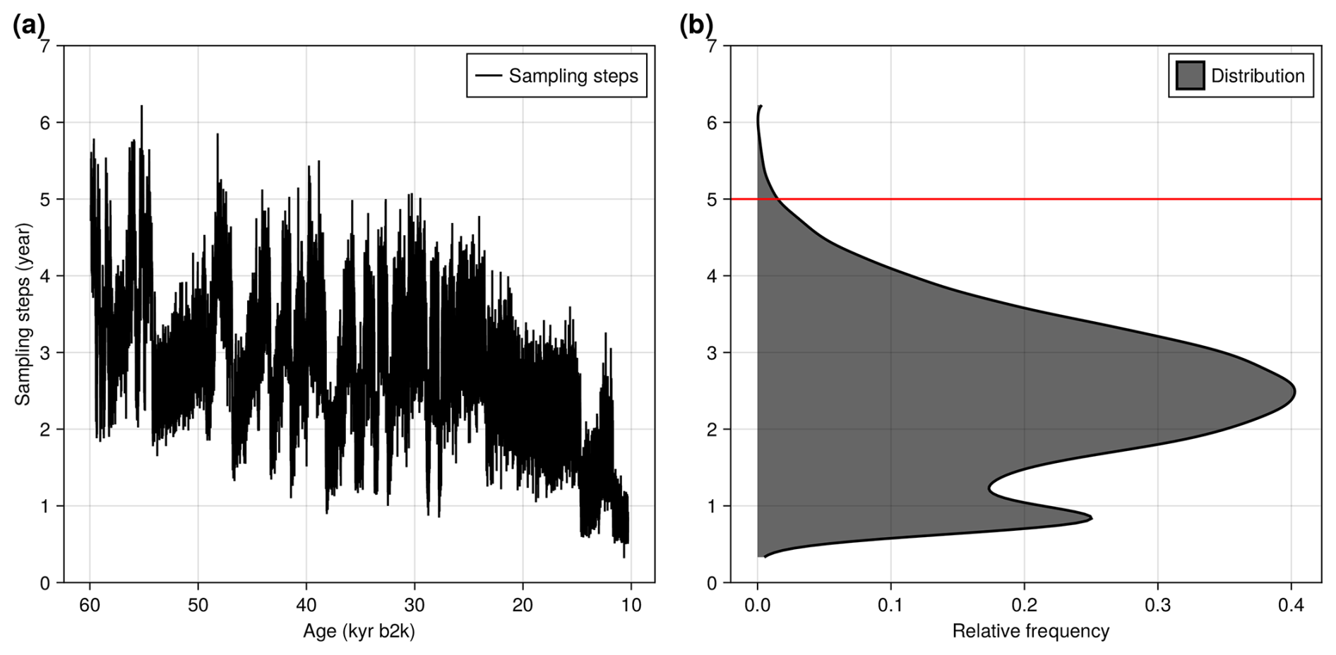
Figure A1 Temporal sampling steps of the raw NGRIP δ¹⁸O record on the GICC05 time scale as a function of time (a) and their distribution (b). The horizontal red line marks the temporal resolution of 5 years.

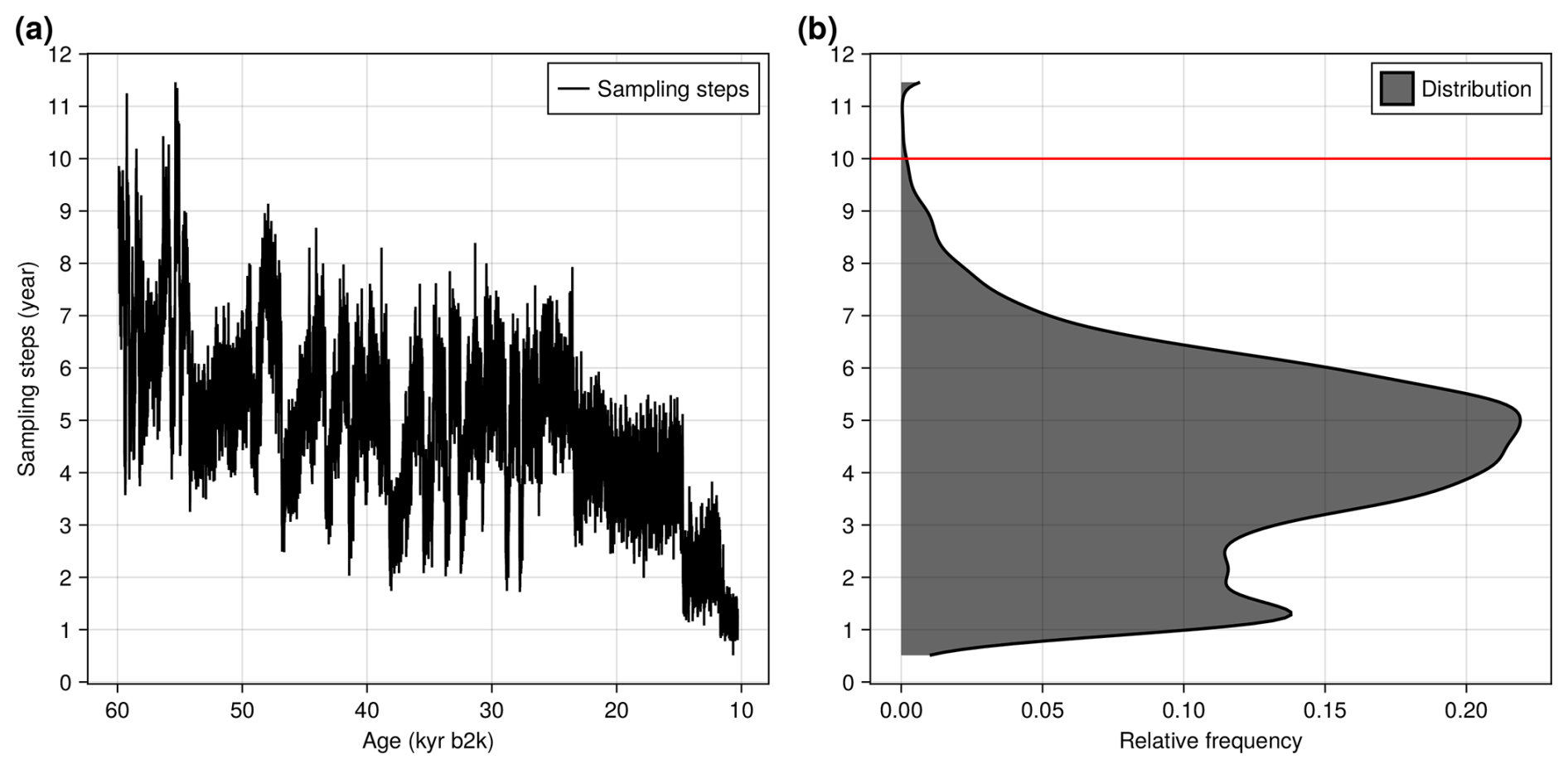
Figure A2 Temporal sampling steps of the raw NEEM δ¹⁸O record on the GICC05 time scale as a function of time (a) and their distribution (b). The horizontal red line marks the temporal resolution of 10 years.

A2 Significance testing

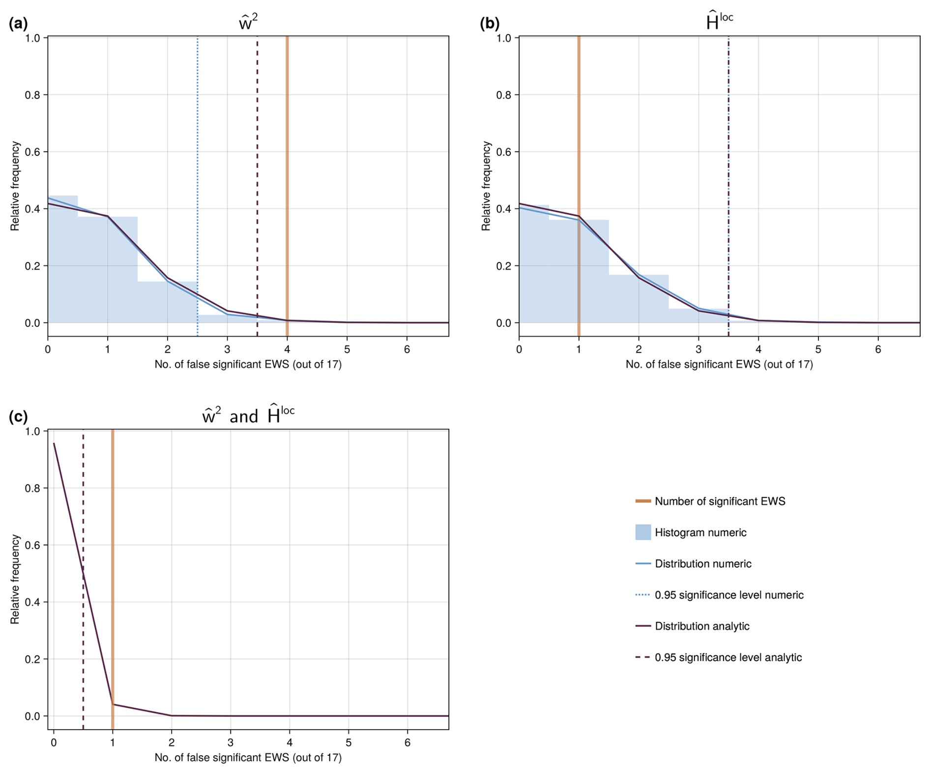
Figure A3 Null-model distributions for the number of significant EWS in ${\widehat{w}}^{\mathrm{2}}$ (a), ${\widehat{H}}^{\text{loc}}$ (b), and both wavelet-based indicators simultaneously (c) for the NGRIP δ¹⁸O record with 5-year resolution.

A3 Wavelet-based EWS

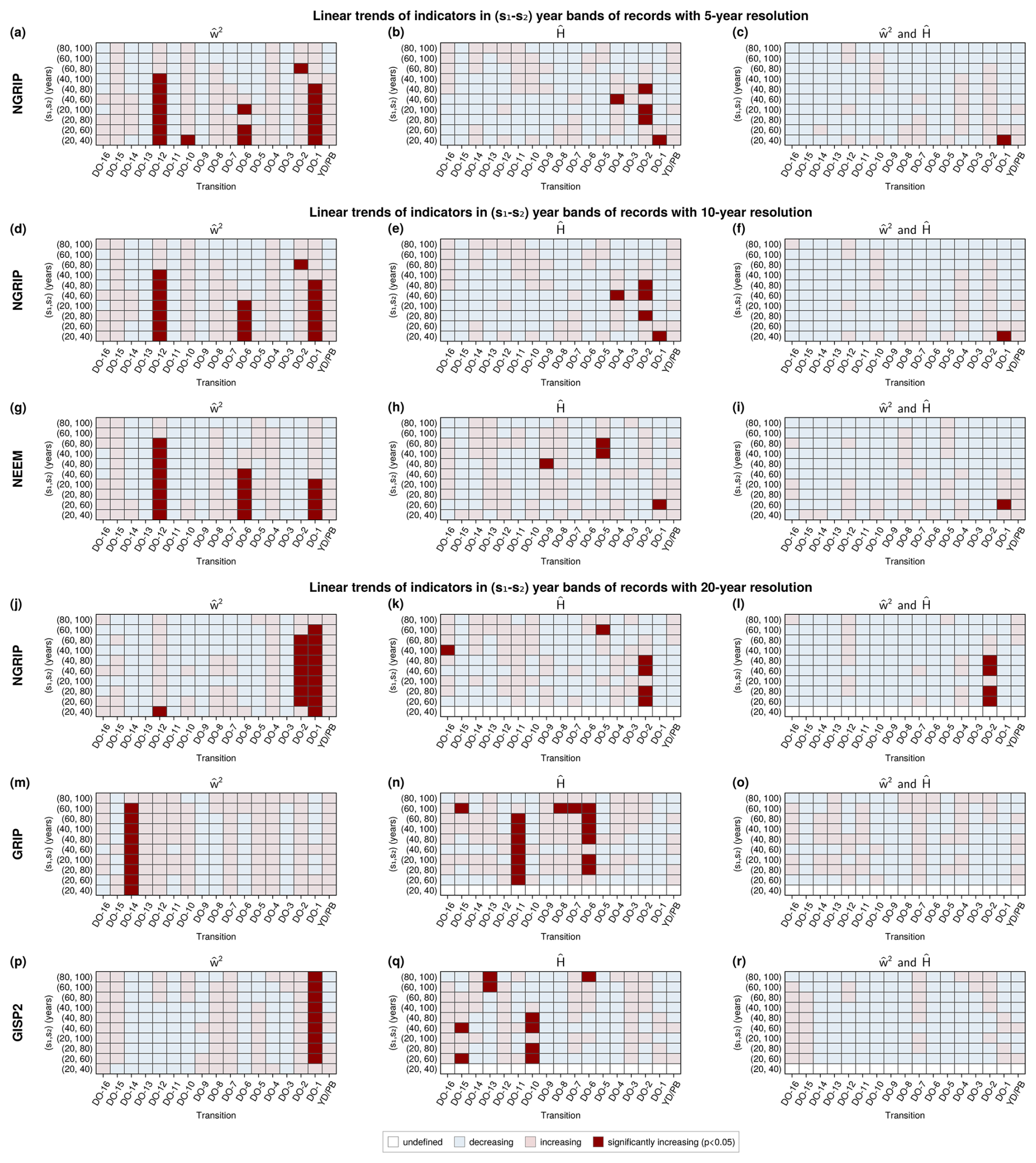
Figure A4 Linear trends of wavelet-based early warning indicators in a selection of scale bands (s₁,s₂) for individual transitions of the NGRIP record in 5- (a–c), 10- (d–f) and 20-year resolution (j–l), NEEM (g–i), GRIP (m–o), and GISP2 (p–r). The direction of trends of the scale-averaged wavelet coefficient are shown in the left (a, d, g, j, m, p), those of the local Hurst exponent in the middle column (b, e, h, k, n, q). The right column (c, f, i, l, o, r) shows an increasing trend if both indicators increase and a decreasing trend otherwise. Significant indicator increases are displayed in dark red.

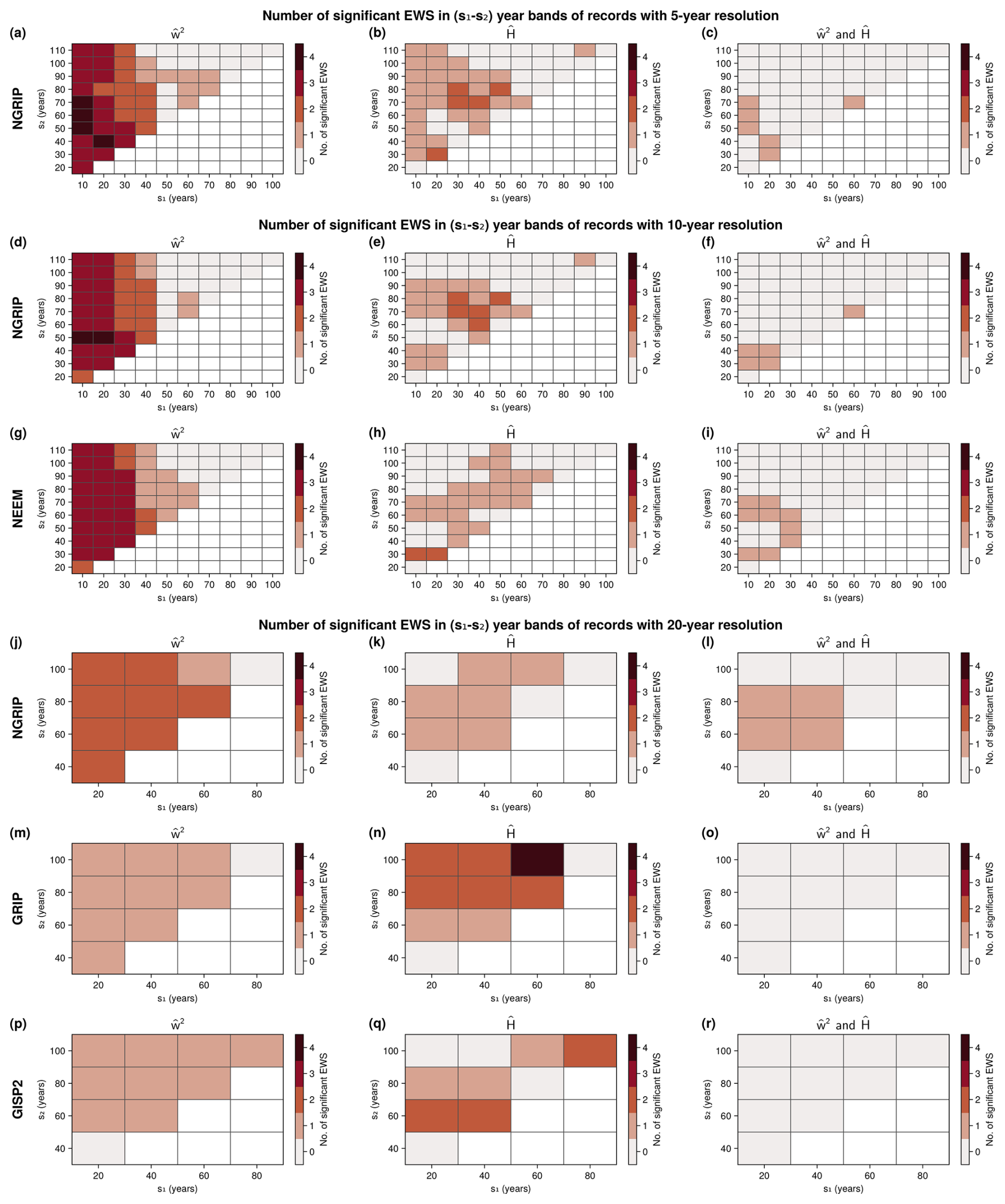
Figure A5 Numbers of significant wavelet-based EWS in different scale bands between s₁ and s₂ years of the NGRIP record in 5- (a–c), 10- (d–f) and 20-year resolution (j–l), NEEM (g–i), GRIP (m–o), and GISP2 (p–r). EWS of the scale-averaged wavelet coefficient are shown in the left (a, d, g, j, m, p), those of the local Hurst exponent in the middle (b, e, h, k, n, q) and of both simultaneously in the right column (c, f, i, l, o, r).