Milankovitch theory “as an initial value problem”: Implications of the long memory of ice advection

We describe a so far unrecognized physical phenomenon of orbital forcing modifying the terrestrial physics in such a way that instead of erasing the memory of the initial conditions this memory is extended and the initial values become major governing parameters. Specifically: The dynamics of large ice sheets is fundamentally defined by the advection of mass and temperature. The timescale of these processes is critically dependent on the surface mass balance. Because of the ice-climate system's nonlinearity, its response to the orbital forcing in terms of the engagement of negative and positive feedbacks is not symmetrical. This asymmetry may reduce the effective mass influx, and the resultant advection timescale may become longer, which is equivalent to the system having a longer memory of its initial conditions. In this case the Milankovitch theory becomes an initial value problem: Depending on the initial conditions, for the same orbital forcing and for the same balance between terrestrial positive and negative feedbacks, the historical glacial rhythmicity could have been dominated either by the eccentricity period of ∼100 kyr, or by the doubled obliquity period of ∼80 kyr, or by a combination of both. In fact, empirical records demonstrate that the dominant period of the Late Pleistocene ice ages evolved from a ∼80 to ∼100 kyr rhythmicity. The quantitative similarity of this dominant-period trajectory and the one, made by the long-memory model, suggests that the records of the Late Pleistocene glacial rhythmicity could have been produced by a long-memory initial-value-dependent climate system, or, in other words, the slopes in empirical dominant-period trajectories are signatures of a long memory.

The scaling law of the dominant-period trajectory provides a theoretical insight into the discovered phenomenon. It reveals that this trajectory is dependent on the memory duration that is sensitive to initial conditions. The sensitivity of the memory duration to the initial values emerges as the result of the system's incomplete similarity in two similarity parameters colliding into one conglomerate similarity parameter that is the ratio of the orbitally modified advection timescale and the orbital period. The critical dependence of this similarity parameter on poorly defined accumulation-minus-ablation mass balance as well as its dependence on the initial values makes ice ages fundamentally difficult to predict. For the same reason, the disambiguation of paleo-records is extremely challenging. The quasi-eccentricity periods produced by the long-memory system in response to pure obliquity forcing make a remarkable example of this challenge because in the time series they may be naively attributed to the eccentricity modulated precession forcing.

The long-memory relaxation time series may have abrupt dominant-periodicity transitions (e.g., from ∼40 to 80 kyr) produced without any changes of parameters. This observation implies that the middle-Pleistocene transition may be a manifestation of the terrestrial long-memory response to the orbital forcing.

1 Introduction

In memory of Barry Saltzman.

Though modelling of the Late Pleistocene ice-age history using space resolving three-dimensional models (e.g., Abe-Ouchi et al., 2013) and models of intermediate complexity (e.g., Ganopolski and Calov, 2011) are now computationally affordable, the dynamical paleoclimatology (the term was coined by Barry Saltzman, 2002) remains to be a powerful and may be even a preferable tool to study climate evolution on orbital timescales. Even if we put aside the esthetical attractiveness of dynamical models (in the sense of Paul Dirac's vision that a physical law must indeed possess mathematical beauty), there are important physical considerations that make them essential. The first fundamental concern, that even three-dimensional models are not able to comprehensively address, relates to the fact that the ice-sheet volume is controlled by a small difference of two big values, accumulation and ablation, and therefore “… in their current state, ice sheet models do not have the predictive power to precisely reconstruct ice sheet history” (Gowan, 2023). The second consideration has been rigorously substantiated by Bahr et al. (2015) in their review and comparison of glaciers' and ice sheets' scaling solutions versus corresponding three-dimensional models: “… if any of the numerical models' parameters are unknown or have a distribution of possible values… there is no a priori reason to expect that a tuned model will be more accurate than a tuned scaling solution”.

These observations are critical for the purpose of our study. Up to date, there are two commonly accepted interpretations of the Milankovitch theory: either ice ages are directly driven by the insolation changes, or they represent the internal property of the terrestrial physics, paced (phase locked) by the orbital forcing (Tziperman et al., 2006). As Tziperman et al. (2006) explain, phase locking requires some kind of dissipation in the terrestrial climate system that erases the memory of initial values from the time series. Does the terrestrial climate system, or more specifically, continental ice sheets, indeed have short memory of the initial values? Since the dynamics of large ice sheets is defined by advection of ice and temperature, the accumulation-minus-ablation mass balance defines the vertical advection timescale and the memory duration. Therefore, three-dimensional models cannot provide us with a definite constraint. Consequently, while Milankovitch theories based on a short-memory terrestrial physics remain viable, the possibility of the terrestrial long-memory climate should not be excluded, especially since such terrestrial systems are well known to exist. For example, Omta et al. (2013, 2016) have demonstrated that the ocean calcifier-alkalinity system has long memory duration and that the asymptotic period of this system, being periodically forced, depends on its initial values.

In this paper, we will discuss to what extent this accumulation-minus-ablation mass influx affects ice-sheet sensitivity to initial values. To introduce the language of our study, we begin with a very simple illustration. Although this linear example is not a complete analogy of highly nonlinear ice-climate system by any means, it will give us an opportunity to introduce concepts of dynamical system memory, memory duration, and memory-duration sensitivity to initial values, as well as the key similarity parameter that defines this sensitivity. With this caveat in mind, let us assume that ice volume x evolves according to the following mass balance:

$$\begin{array}{}\text{(1)}& {\displaystyle \frac{\mathrm{d}x}{\mathrm{d}t}}=a-{\displaystyle \frac{x}{\mathit{\tau }}}\end{array}$$

with the initial condition x=x₀ when t=0. Here a is the terrestrial mass influx (accumulation minus ablation) and τ is the ice-sheet dynamical timescale. The adimensional solution of this equation is:

$$\begin{array}{}\text{(2)}& {\displaystyle \frac{x}{a\mathit{\tau }}}=\left({\displaystyle \frac{x_{\mathrm{0}}}{a\mathit{\tau }}}-\mathrm{1}\right)e^{-\frac{t}{\mathit{\tau }}}+\mathrm{1}\end{array}$$

Several observations will be useful for our further discussion:

1. The term $\left(\frac{x_{\mathrm{0}}}{a\mathit{\tau }}-\mathrm{1}\right)e^{-\frac{t}{\mathit{\tau }}}$ is the decaying memory of the dynamical system (1) about its initial conditions;

2. The memory duration M can be defined as the time needed by the system to get within a given distance m≪1 from the steady state, i.e., $\frac{M}{\mathit{\tau }}=\ln \left[\frac{\mathrm{1}}{m}\left(\frac{x_{\mathrm{0}}}{a\mathit{\tau }}-\mathrm{1}\right)\right]$. It is thus fully defined by the dynamical properties of the system, i.e., the timescale τ, and by the adimensional similarity parameter $C=\frac{x_{\mathrm{0}}}{a\mathit{\tau }}$ that is the ratio of the vertical advection timescale $\frac{x_{\mathrm{0}}}{a}$ and τ;

3. The systems with strong negative feedbacks (τ→0) have short memories and are initial-value independent: i.e., lim${}_{\mathit{\tau }\to \mathrm{0}}M=\mathrm{0}$;

4. In a long-memory system, the time series are initial-value dependent. Even so, the memory duration may be either sensitive to initial values or initial-values independent. If the mass influx is strong, then the advection timescale $\frac{x_{\mathrm{0}}}{a}$ is short relative to τ, i.e., C≪1, and the memory duration is independent on initial values. A weak mass influx makes the advection timescale $\frac{x_{\mathrm{0}}}{a}$ longer such that C∼1 and the memory duration becomes initial-value sensitive;

5. The steady-state x=aτ may be reproduced by a short- or long-memory system if its mass balance a is adjusted accordingly. Therefore, any claim that nature is not sensitive to initial conditions because a short-memory model has successfully reproduced a sample time series, should be taken cautiously unless our knowledge about mass balance and internal dynamics is unambiguous. As we already know, this is not the case.

The dynamics of a real ice sheet, approximated as the thin viscous boundary layer of ice media, is largely defined by the advection of mass and temperature. The timescale of these processes is not fixed, but instead it is critically dependent on the surface mass balance, that is an outcome of a sophisticated interplay of orbital forcing and internal dynamics. In our following presentation, we will, first, describe our model and demonstrate that when the orbital forcing is neither strong enough to engage sufficient positive feedbacks, nor small enough to be overwhelmed by the terrestrial mass influx, the resultant effective mass influx affected by negative feedbacks may become smaller, the advection timescale may become longer and this is equivalent to longer and initial-values dependent memory duration. Thus the theory of the Pleistocene glacial rhythmicity, i.e., the Milankovitch theory, becomes an initial value problem. Though the title of our paper obviously alludes to Saltzman's (1962) landmark work, we do not necessarily anticipate identifying deterministic chaos in the physical model of an ice sheet. We will demonstrate though that, depending on initial conditions, for the same periodicity of the orbital forcing, the Pleistocene glacial rhythmicity could have been dominated either by the eccentricity period of ∼100 kyr, or by the doubled obliquity period of ∼80 kyr, or by a combination of both. We will also show that a particular trajectory of the dominant period produced by a long-memory model may be reasonably close to the empirical data and therefore the empirical records of the Late Pleistocene glacial rhythmicity could have been produced by a long-memory initial-value dependent climate system.

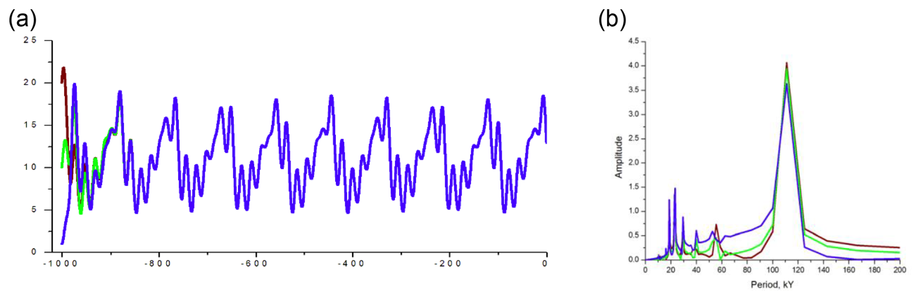
Figure 1 The dynamical system response to pure eccentricity-modulated precession $F=\mathrm{1}\left[\sin \left(\frac{\mathrm{2}\mathit{\pi }t}{\mathrm{19}}\right)+\sin \left(\frac{\mathrm{2}\mathit{\pi }t}{\mathrm{23}}\right)\right]$. Here (a) the time series (kyr before present) of the area of glaciation in (10⁶ km²) and (b) corresponding spectral diagrams; brown is for $S\left(\mathrm{0}\right)=\mathrm{20}\times {\mathrm{10}}^{\mathrm{6}}$ km²; green is for $S\left(\mathrm{0}\right)=\mathrm{10}\times {\mathrm{10}}^{\mathrm{6}}$ km²; blue is for $S\left(\mathrm{0}\right)=\mathrm{1}\times {\mathrm{10}}^{\mathrm{6}}$ km².

To provide theoretical insight into the discovered phenomenon, we will then derive the scaling law of the dominant-period trajectory. The law will reveal that this trajectory is dependent on memory duration that is sensitive to initial conditions. The sensitivity of the memory duration to initial values emerges as the result of system's incomplete similarity in two similarity parameters colliding into one conglomerate similarity parameter that is the ratio of the orbitally modified advection timescale and the orbital period. The critical dependence of this similarity parameter on the poorly defined accumulation-minus-ablation mass balance as well as its dependence on initial values makes ice ages fundamentally difficult to predict. For the same reason, disambiguation of paleo-records is extremely challenging. We will illustrate this challenge with a remarkable phenomenon of quasi-eccentricity periods produced by the long-memory system in response to pure obliquity forcing. Finally, we will demonstrate that the long-memory relaxation time series may have abrupt dominant-periodicity transitions (e.g., from ∼40 to 80 kyr) produced without any changes of parameters. The phase locking in these time series may be delayed and therefore the middle-Pleistocene transition may be a manifestation of the terrestrial long-memory delayed-phase-locking response to the orbital forcing.

2 The observations

In our previous work, we derived a dynamical model of glacial rhythmicity based on scaled mass-, momentum-, and heat-conservation equations of non-Newtonian ice flow combined with the energy-balance model of global climate (Verbitsky et al., 2018, VCV18 thereafter, Verbitsky and Crucifix, 2020, 2023; Verbitsky, 2022):

$$\begin{array}{}\text{(3)}& {\displaystyle \frac{\mathrm{d}S}{\mathrm{d}t}}={\displaystyle \frac{\mathrm{4}}{\mathrm{5}}}{\mathit{\zeta }}^{-\mathrm{1}}{S}^{\mathrm{3}/\mathrm{4}}\left(\widehat{a}-\mathit{\epsilon }F-\mathit{\kappa }\mathit{\omega }-c\mathit{\theta }\right)\text{(4)}& {\displaystyle \frac{\mathrm{d}\mathit{\theta }}{\mathrm{d}t}}={\mathit{\zeta }}^{-\mathrm{1}}{S}^{-\mathrm{1}/\mathrm{4}}\left(\widehat{a}-\mathit{\epsilon }F-\mathit{\kappa }\mathit{\omega }\right)\left\{\mathit{\alpha }\mathit{\omega }+\mathit{\beta }\left[S-S_{\mathrm{0}}\right]-\mathit{\theta }\right\}\text{(5)}& {\displaystyle \frac{\mathrm{d}\mathit{\omega }}{\mathrm{d}t}}=-\mathit{\gamma }\left[S-S_{\mathrm{0}}\right]-{\displaystyle \frac{\mathit{\omega }}{{\mathit{\tau }}_{\mathit{\omega }}}}\end{array}$$

Here, S (m²) is the area of an ice sheet, θ (°C) is the ice-sheet basal temperature, and ω (°C) is the global “rest-of-the-climate” temperature. Equation (3) is the ice mass balance $\frac{\mathrm{d}\left(HS\right)}{\mathrm{d}t}=AS$, where the ice thickness H is determined from the thin-viscous-boundary-layer approximation of ice flow, $H=\mathit{\zeta }{S}^{\mathrm{1}/\mathrm{4}}$, ζ is dimensional (m${}^{\mathrm{1}/\mathrm{2}}$) factor (Verbitsky, 1992) and $A=\widehat{a}-\mathit{\epsilon }F-\mathit{\kappa }\mathit{\omega }-c\mathit{\theta }$ is the surface mass influx. Equation (4) describes vertical ice-temperature advection and Eq. (5) is the climate energy-balance equation. More specifically, $\widehat{a}$ (m s⁻¹) is the snow precipitation rate; F is adimensional external forcing of the amplitude ε (m s⁻¹); κω is “fast” positive feedback of the global climate in ice mass balance; cθ represents ice-sheet basal sliding combining positive feedback, αω, and a negative feedback β[S−S₀] (both are “slow” due to the vertical temperature advection). The term $-\mathit{\gamma }\left[S-S_{\mathrm{0}}\right]$ is albedo forcing for global temperature. Remaining parameters κ (m s⁻¹ °C⁻¹), c (m s⁻¹ °C⁻¹), α (adimensional), β (°C m⁻²) and γ (°C m⁻² s⁻¹) are sensitivity coefficients; S₀ (m²) is a reference glaciation area; and τ_ω (s) is the global-temperature timescale.

We have demonstrated (Verbitsky and Crucifix, 2020) that the dynamical properties of the system (3)–(5) can be largely defined by only two similarity parameters: (a) the ratio of the orbital forcing amplitude to the amplitude of the terrestrial mass influx, $\frac{\mathit{\epsilon }}{\widehat{a}}$ , and (b) the so called V-number that is the ratio of terrestrial positive-to-negative feedbacks amplitudes.

$$\begin{array}{}\text{(6)}& {\displaystyle \frac{P}{T}}={\mathrm{\Phi }}_{\mathrm{o}}\left({\displaystyle \frac{\mathit{\epsilon }}{\widehat{a}}},V\right)\end{array}$$

Here P is the dominant period of the system response, and T is the forcing period. Specifically, when the ratio of the orbital forcing amplitude to the amplitude of the terrestrial mass influx is about 1.5–2, and the positive feedbacks in the system are well articulated, i.e., V ∼0.7–1, the system produces the obliquity-period doubling bifurcation. It is important to note that for the reference values of the VCV18 parameters the scaling law (6) is initial-values independent or in other words the system (3)–(5) has a short memory of its initial values.

Although the astronomical forcing is the result of celestial mechanics, and the orbital periods such as the precession, obliquity, and eccentricity periods are generally accepted almost like physical constants, the amplitude of this forcing, as a component of the global ice mass balance, is defined much less precisely. Therefore, it appears of considerable interest to study the sensitivity of the system's dynamical behavior to the amplitude of the imposed orbital forcing.

For the purpose of this study, all model parameters are fixed at their reference VCV18 values, such that in all experiments V=0.75, i.e., the terrestrial positive feedbacks are well articulated relative to the negative feedbacks. The only values that are going to be changed will be the initial area of an ice sheet S(0) (10⁶ km²) and the adimensional amplitude of the astronomical forcing that, instead of the mid-June insolation at 65° latitude, used in VCV18, will be modeled as the following:

$$\begin{array}{}\text{(7)}& F={\mathit{\epsilon }}_{\mathrm{p}}\left[\sin \left({\displaystyle \frac{\mathrm{2}\mathit{\pi }t}{\mathrm{19}}}\right)+\sin \left({\displaystyle \frac{\mathrm{2}\mathit{\pi }t}{\mathrm{23}}}\right)\right]+{\mathit{\epsilon }}_{\mathrm{o}}\sin \left({\displaystyle \frac{\mathrm{2}\mathit{\pi }t}{\mathrm{41}}}\right)\end{array}$$

Here t (kyr) is time, and ε_p and ε_o are adimensional amplitudes of the precession and obliquity correspondingly. The first two terms replicate eccentricity-modulated precession, and the last term represents the obliquity forcing. We will now describe five numerical experiments. In these experiments, we will be especially observant of the dominant-period sensitivity to the initial values.

2.1 Pure eccentricity-modulated precession, $F=\mathrm{1}\left[\sin \left(\frac{\mathrm{2}\mathit{\pi }t}{\mathrm{19}}\right)+\sin \left(\frac{\mathrm{2}\mathit{\pi }t}{\mathrm{23}}\right)\right]$

The results of the first experiment are presented in Fig. 1.

Without obliquity, the system response is dominated by the eccentricity period (∼110 kyr in our case). Most importantly, though the time series are obviously not identical for different initial conditions, the dominant period of the system response is independent of the initial conditions. The memory duration of the system about its initial conditions does not exceed ∼100 kyr.

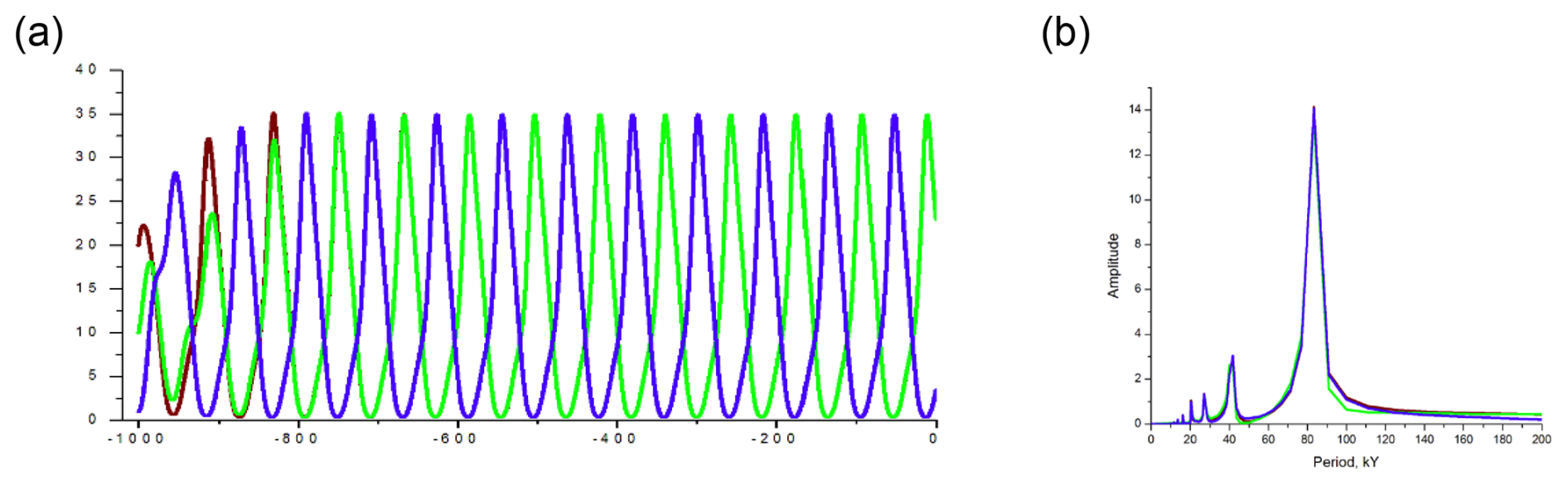
Figure 2 The dynamical system response to pure obliquity forcing, $F=\mathrm{1.0}\sin \left(\frac{\mathrm{2}\mathit{\pi }t}{\mathrm{41}}\right)$. Here (a) the time series (kyr before present) of the area of glaciation in (10⁶ km²) and (b) corresponding spectral diagrams; brown is for $S\left(\mathrm{0}\right)=\mathrm{20}\times {\mathrm{10}}^{\mathrm{6}}$ km²; green is for $S\left(\mathrm{0}\right)=\mathrm{10}\times {\mathrm{10}}^{\mathrm{6}}$ km²; blue is for $S\left(\mathrm{0}\right)=\mathrm{1}\times {\mathrm{10}}^{\mathrm{6}}$ km².

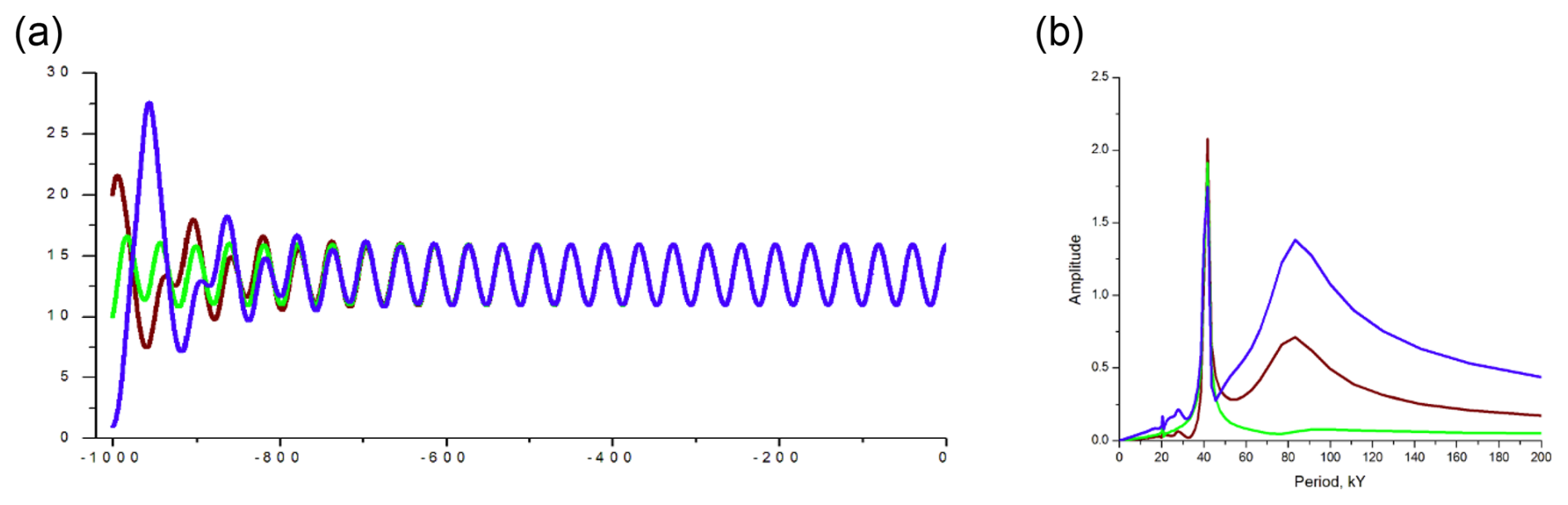
Figure 3 The dynamical system response to pure obliquity forcing, $F=\mathrm{0.5}\sin \left(\frac{\mathrm{2}\mathit{\pi }t}{\mathrm{41}}\right)$. Here (a) the time series (kyr before present) of the area of glaciation in (10⁶ km²) and (b) corresponding spectral diagrams; brown is for $S\left(\mathrm{0}\right)=\mathrm{20}\times {\mathrm{10}}^{\mathrm{6}}$ km²; green is for $S\left(\mathrm{0}\right)=\mathrm{10}\times {\mathrm{10}}^{\mathrm{6}}$ km²; blue is for $S\left(\mathrm{0}\right)=\mathrm{1}\times {\mathrm{10}}^{\mathrm{6}}$ km².

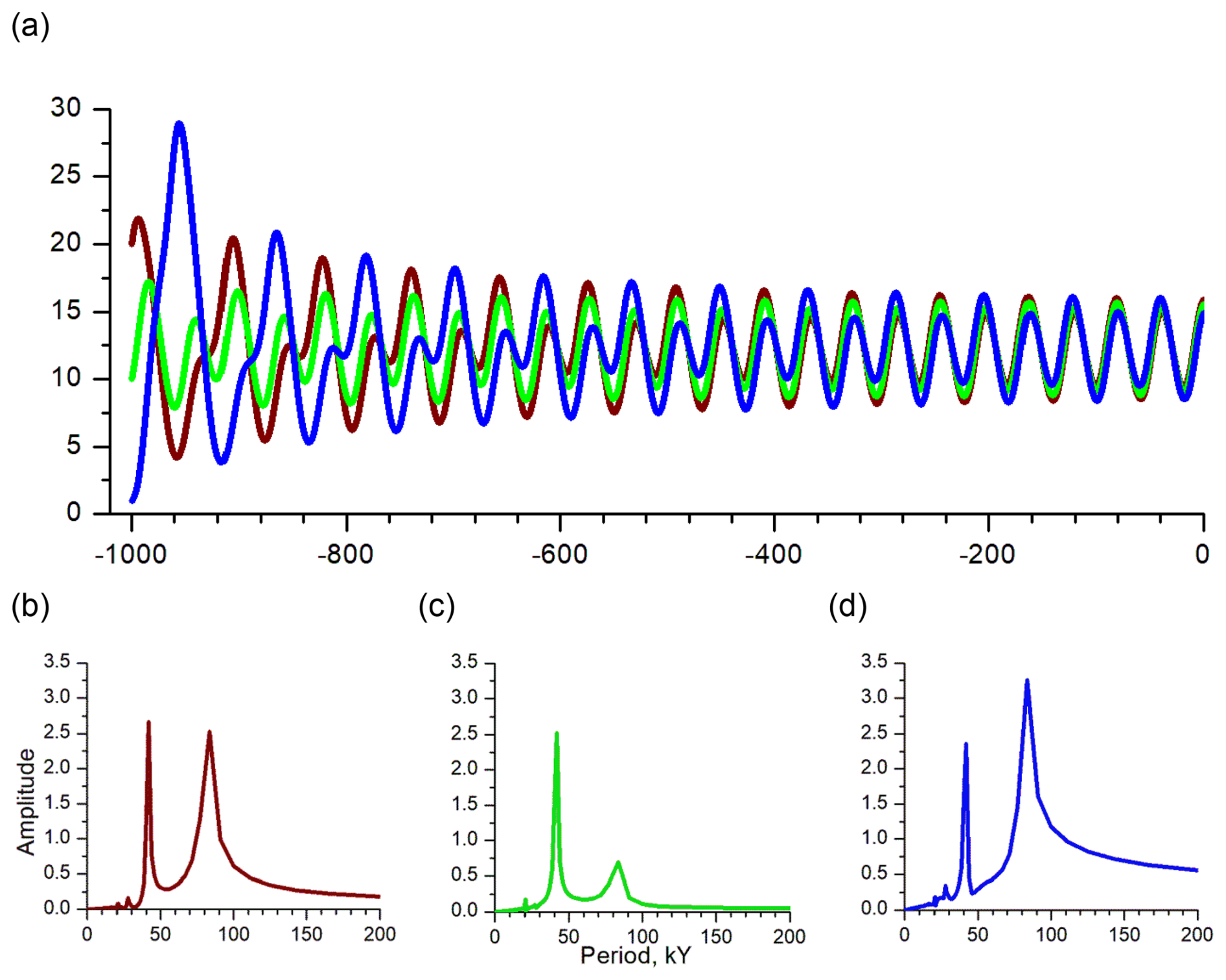
Figure 4 The dynamical system response to pure obliquity forcing, $F=\mathrm{0.7}\sin \left(\frac{\mathrm{2}\mathit{\pi }t}{\mathrm{41}}\right)$. Here (a) the time series (kyr before present) of the area of glaciation in (10⁶ km²) and (b–d) corresponding spectral diagrams; brown is for $S\left(\mathrm{0}\right)=\mathrm{20}\times {\mathrm{10}}^{\mathrm{6}}$ km²; green is for $S\left(\mathrm{0}\right)=\mathrm{10}\times {\mathrm{10}}^{\mathrm{6}}$ km²; blue is for $S\left(\mathrm{0}\right)=\mathrm{1}\times {\mathrm{10}}^{\mathrm{6}}$ km².

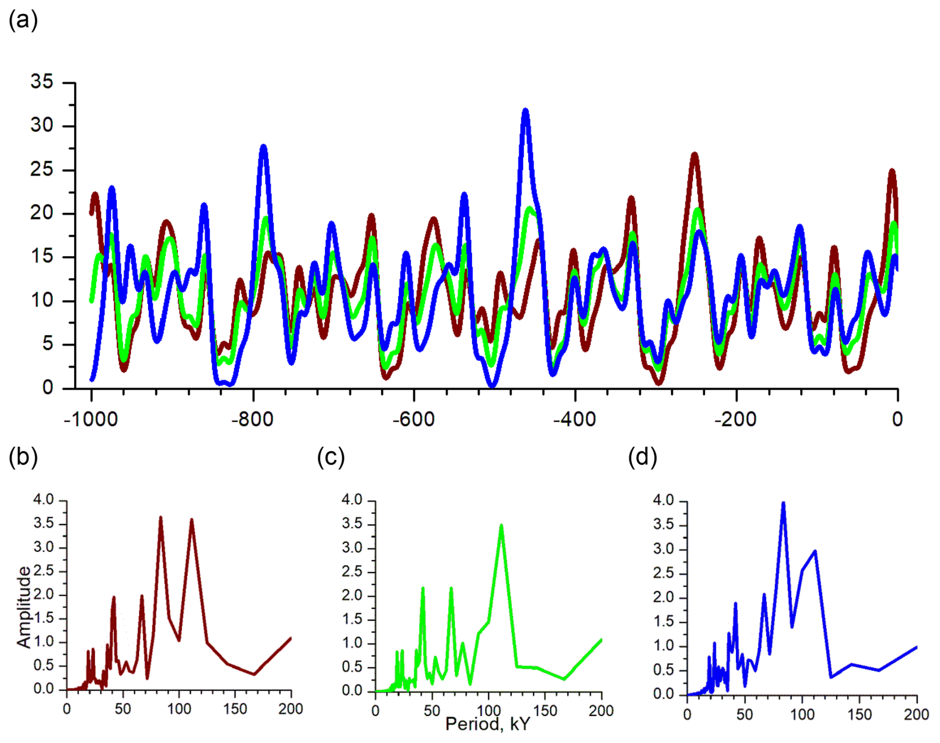
Figure 5 The dynamical system response to orbital forcing, $F=\mathrm{0.7}\left[\sin \left(\frac{\mathrm{2}\mathit{\pi }t}{\mathrm{19}}\right)+\sin \left(\frac{\mathrm{2}\mathit{\pi }t}{\mathrm{23}}\right)\right]+\mathrm{0.7}\sin \left(\frac{\mathrm{2}\mathit{\pi }t}{\mathrm{41}}\right)$. Here (a) the time series (kyr before present) of the area of glaciation in (10⁶ km²) and (b–d) corresponding spectral diagrams; brown is for $S\left(\mathrm{0}\right)=\mathrm{20}\times {\mathrm{10}}^{\mathrm{6}}$ km²; green is for $S\left(\mathrm{0}\right)=\mathrm{10}\times {\mathrm{10}}^{\mathrm{6}}$ km²; blue is for $S\left(\mathrm{0}\right)=\mathrm{1}\times {\mathrm{10}}^{\mathrm{6}}$ km².

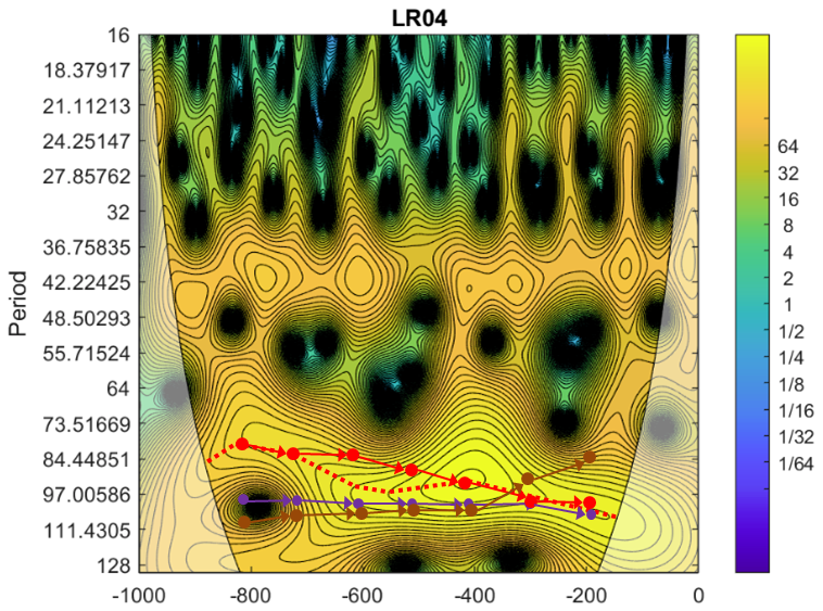
Figure 6 The evolution of the ice volume wavelet spectra over the past 1000 kyr based on Lisiecki and Raymo (2005, “LR04” stack) benthic foraminifera δ¹⁸O data. The color scale shows wavelet amplitude and the dotted red line displays the trajectory of the LR04 dominant period. The circled red line represents the trajectory of the dominant period for the long-memory-model solution shown in Fig. 5 with $S\left(\mathrm{0}\right)=\mathrm{1}\times {\mathrm{10}}^{\mathrm{6}}$ km²; the circled purple line represents the trajectory of the dominant period for the model solution with $S\left(\mathrm{0}\right)=\mathrm{10}\times {\mathrm{10}}^{\mathrm{6}}$ km²; and the circled brown line represents the trajectory of the dominant period for the long-memory-model solution with $S\left(\mathrm{0}\right)=\mathrm{20}\times {\mathrm{10}}^{\mathrm{6}}$ km².

2.2 Pure obliquity forcing, $F={\mathit{\epsilon }}_{\mathrm{o}}\sin \left(\frac{\mathrm{2}\mathit{\pi }t}{\mathrm{41}}\right)$

The results of the next three experiments are presented in Figs. 2–4. Consistently with VCV18, when terrestrial positive feedbacks are well articulated (V=0.75) and the amplitude of the obliquity forcing is strong enough (ε_o=1, Fig. 2), the system exhibits the obliquity-period doubling bifurcation. The dominant period of the system response (∼80 kyr) is not sensitive to the initial conditions. Also similar to VCV18, when terrestrial positive feedbacks are still strong (V=0.75) but the amplitude of the obliquity forcing is relatively weak (ε_o=0.5, Fig. 3), the system does not bifurcate. The dominant period of the system response (∼40 kyr) is not sensitive to the initial conditions either.

While the experiments described above (Figs. 1–3) demonstrate the short memory of the climate system involved and may be interpreted as a classical non-linear phase locking to orbital forcing (Tziperman et al, 2006), the most interesting behavior of the system is presented in Fig. 4 (ε_o=0.7). It can be observed that, when the orbital forcing is of intermediate intensity, the phase locking is delayed because the relaxation timescale may become much longer that is equivalent to longer system's memory of its initial conditions. Remarkably, the memory duration and the dominant period of fluctuations become sensitive to the initial conditions, and the dominant period may be either of the obliquity-period or of the double-obliquity-period value.

This intriguing phenomenon needs a physical explanation. Though more rigorous reasoning will be presented in the next Sect. 3 with the scaling law, some preliminary simple considerations may also be appropriate. Because of the system's nonlinearity, its response to the orbital forcing in terms of engagement of negative and positive feedbacks is not symmetrical. In the VCV18 model (VCV18, Eq. 30), this may be observed as a shift of the time-mean glaciation area 〈S〉 that is dependent on the effective mass influx, i.e., $\langle S\rangle =S_{\mathrm{0}}+\frac{\widehat{a}}{\mathit{\beta }c(\mathrm{1}-V)}$. For example, for the reference values of model parameters and without astronomical forcing, the equilibrium glaciation area $S=\mathrm{15}\times {\mathrm{10}}^{\mathrm{6}}$ km², because $S_{\mathrm{0}}=\mathrm{12}\times {\mathrm{10}}^{\mathrm{6}}$ km², and $\frac{\widehat{a}}{\mathit{\beta }c(\mathrm{1}-V)}=\mathrm{3}\times {\mathrm{10}}^{\mathrm{6}}$ km². The obliquity forcing of a relatively small amplitude (ε_o=0.5, Fig. 3) does not engage sufficient positive feedback (due to vertical temperature advection that is period-sensitive and behaves like a lower-frequency filter) and the dominant negative feedbacks shift the mean glaciation area to $S=\mathrm{13.5}\times {\mathrm{10}}^{\mathrm{6}}$ km². In the VCV18 model, this is equivalent to 50 % reduction in the mean terrestrial mass influx. The obliquity forcing of a large amplitude (ε_o=1, Fig. 2) administers strong positive feedbacks and shifts the mean glaciation area to $S=\mathrm{17.7}\times {\mathrm{10}}^{\mathrm{6}}$ km² that is equivalent to an almost doubled mean terrestrial mass influx. The obliquity forcing of an intermediate amplitude (ε_o=0.7, Fig. 4) shifts the mean glaciation area to 12.3×10⁶ km² which is equivalent to the significant, a 10-fold, reduction of the terrestrial mass influx. Indeed, the actual mass influx, the right-hand side of the Eq. (3), is formed as an output of a sophisticated interplay of the mass influx $\widehat{a}$, external forcing, and positive and negative feedbacks. Nevertheless, changes in the equilibrium glaciation area may serve as a qualitative but still insightful indicator of the surface mass-balance changes.

The timescale of the advection processes in the “thin” (relative to its horizontal size) ice sheet can be estimated as $\mathit{\tau }=\frac{H}{\stackrel{\mathrm{̃}}{A}}$, where H is the characteristic ice thickness and $\stackrel{\mathrm{̃}}{A}$ is the mean terrestrial mass influx. Since $H\sim S^{\mathrm{1}/\mathrm{4}}$, the timescale in the described experiments is mostly defined by the effective mass influx, and the 10-fold reduction of it means 10-fold longer vertical-advection timescale and, consequently, ten-fold longer system's memory of its initial conditions. Without astronomical forcing, the relaxation process in the VCV18 dynamical system takes about 100 kyr. The ten-time extension of it implies that the initial conditions of the ice-climate system may be remembered through the entire Late Pleistocene.

2.3 Eccentricity-modulated precession and obliquity forcing of intermediate intensity, $F=\mathrm{0.7}\left[\sin \left(\frac{\mathrm{2}\mathit{\pi }t}{\mathrm{19}}\right)+\sin \left(\frac{\mathrm{2}\mathit{\pi }t}{\mathrm{23}}\right)\right]+\mathrm{0.7}\sin \left(\frac{\mathrm{2}\mathit{\pi }t}{\mathrm{41}}\right)$

When the system is forced by a combination of eccentricity-modulated precession and obliquity, both with intermediate values of their amplitudes, ${\mathit{\epsilon }}_{\mathrm{p}}={\mathit{\epsilon }}_{\mathrm{o}}=\mathrm{0.7}$, the system response, depending on initial conditions, may be dominated either by the eccentricity period of ∼100 kyr, or by the doubled obliquity period of ∼80 kyr, or by a combination of both (Fig. 5).

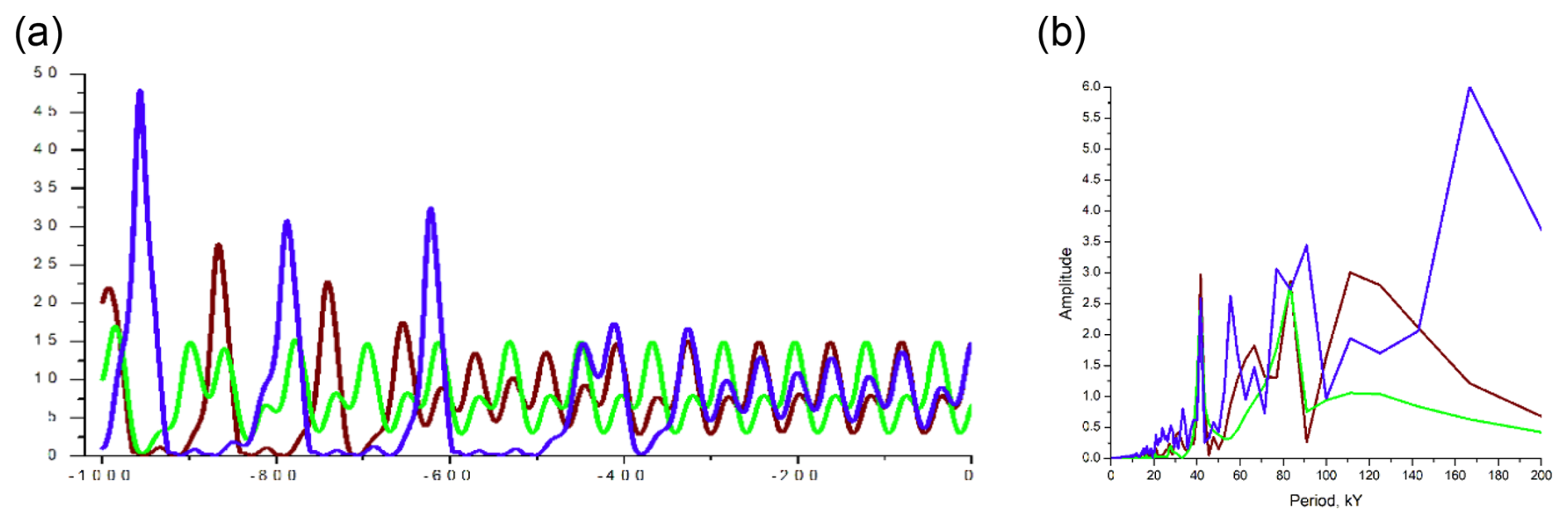
Figure 7 The dynamical system response to pure obliquity forcing, $F=\mathrm{1}\sin \left(\frac{\mathrm{2}\mathit{\pi }t}{\mathrm{41}}\right)$, $\widehat{a}=\mathrm{0.035}$. Here (a) the time series (kyr before present) of the area of glaciation in (10⁶ km²) and (b) corresponding spectral diagrams; brown is for $S\left(\mathrm{0}\right)=\mathrm{20}\times {\mathrm{10}}^{\mathrm{6}}$ km²; green is for $S\left(\mathrm{0}\right)=\mathrm{10}\times {\mathrm{10}}^{\mathrm{6}}$ km²; blue is for $S\left(\mathrm{0}\right)=\mathrm{1}\times {\mathrm{10}}^{\mathrm{6}}$ km².

Figure 6 shows the high-resolution evolution of the ice volume wavelet spectra over the past 1000 kyr based on Lisiecki and Raymo (2005) benthic foraminifera δ¹⁸O data.

The empirical trajectory of the dominant period of the ice-volume variations has a well-articulated slope and therefore infers that the Late Pleistocene glacial rhythmicity evolved from the dominant 80-kyr periods to about 100-kyr periodicity. It is interesting that one of the long-memory-model trajectories (i.e., the one starting from the $S\left(\mathrm{0}\right)=\mathrm{1}\times {\mathrm{10}}^{\mathrm{6}}$ km² initial conditions, Fig. 5) replicates reasonably well this evolving-rhythmicity slope. As we have already mentioned, all model parameters have been fixed to the VCV18 reference values, and therefore we didn't make any additional efforts to achieve a better fit to the empirical data. Nevertheless, the similarity of the empirical and one of the model-made dominant-period trajectories, strongly suggests that the records of the Late Pleistocene glacial rhythmicity could have been produced by a long-memory climate system.

3 The scaling law of the dominant-period trajectory: Why could ice ages be unpredictable?

We will now derive the scaling law that controls the dominant-period trajectory. Without orbital forcing and for fixed balance between positive and negative feedbacks (V=const) the memory duration of the system (3)–(5) depends on only two parameters, $\widehat{a}$ and ζ. This should not come as a surprise. Indeed, these are the parameters that define the timescale of vertical advection, i.e., parameter ζ defines the thickness of an ice sheet for given area S ($H=\mathit{\zeta }{S}^{\mathrm{1}/\mathrm{4}}$) and $\widehat{a}$ is the snowfall rate. Thus, the memory duration M, measured in units of time, can be described as

$$\begin{array}{}\text{(8)}& M=\mathit{\phi }(\mathit{\zeta },\widehat{a},V)\end{array}$$

Here V is adimensional, and parameters ζ (m${}^{\mathrm{1}/\mathrm{2}}$), $\widehat{a}$ (m s⁻¹) have independent dimensions; therefore after applying π-theorem (Buckingham, 1914) to Eq. (8), we can see that the memory duration M of our system, without orbital forcing, is fully described by the timescale $\frac{{\mathit{\zeta }}^{\mathrm{2}}}{\widehat{a}}$ and the V-number:

$$\begin{array}{}\text{(9)}& M={\displaystyle \frac{{\mathit{\zeta }}^{\mathrm{2}}}{\widehat{a}}}{\mathrm{\Phi }}_M\left(V\right)\end{array}$$

Remarkably, without astronomical forcing, the memory duration of our dynamical system does not depend on the initial conditions S(0), or speaking formally, the system has complete similarity in similarity parameter $C=\frac{{\mathit{\zeta }}^{\mathrm{4}}}{S\left(\mathrm{0}\right)}\sim {\mathrm{10}}^{-\mathrm{13}}$ (Barenblatt, 2003). It is important to note that in this case, without orbital forcing, the memory may still be long, and the time series will depend on the initial conditions; it is the memory duration that is independent of initial values.

As we have already observed, the orbital forcing may affect the system's memory. Moreover, we observed that the memory duration may become sensitive to the initial conditions. Therefore the memory duration M of the full system (3)–(5) will depend on the parameters that define its internal memory span, as well as on, generally speaking, initial conditions S(0) and on the amplitude and the period of the astronomical forcing:

$$\begin{array}{}\text{(10)}& M=\mathit{\phi }\left[V,{\displaystyle \frac{{\mathit{\zeta }}^{\mathrm{2}}}{\widehat{a}}},\mathit{\epsilon },T,S\left(\mathrm{0}\right)\right]\end{array}$$

If we choose ε (m s⁻¹), T (s) as parameters with independent dimensions, then, after applying π-theorem, we can state that:

$$\begin{array}{}\text{(11)}& {\displaystyle \frac{M}{T}}={\mathrm{\Phi }}_M\left[V,{\displaystyle \frac{{\mathit{\zeta }}^{\mathrm{2}}}{\widehat{a}T}},{\displaystyle \frac{S\left(\mathrm{0}\right)}{{\mathit{\epsilon }}^{\mathrm{2}}{T}^{\mathrm{2}}}}\right]\end{array}$$

As we have already learned, a weakened mass influx affects the memory. It means that the terrestrial mass influx $\widehat{a}$ may also play a role in the appearance and disappearance of M-span sensitivity to the initial conditions. Indeed, this is the case. In Fig. 7 we show the dynamical system response to the pure obliquity forcing, when ε_o=1 and $\widehat{a}=\mathrm{0.035}$ km kyr⁻¹ instead of VCV18 reference value $\widehat{a}=\mathrm{0.065}$ km kyr⁻¹. It can be observed that the memory duration Min this case is sensitive to initial conditions. Therefore, parameters $\widehat{a}$ and S(0) should be components of the same similarity parameter. This may only happen if the similarity parameters $\frac{{\mathit{\zeta }}^{\mathrm{2}}}{\widehat{a}T}$ and $\frac{S\left(\mathrm{0}\right)}{{\mathit{\epsilon }}^{\mathrm{2}}{T}^{\mathrm{2}}}$ form a conglomerate similarity parameter C, such as:

$$\begin{array}{}\text{(12)}& C={\left({\displaystyle \frac{{\mathit{\zeta }}^{\mathrm{2}}}{\widehat{a}T}}\right)}^{\mathit{\mu }}{\left[{\displaystyle \frac{S\left(\mathrm{0}\right)}{{\mathit{\epsilon }}^{\mathrm{2}}{T}^{\mathrm{2}}}}\right]}^{\mathit{\nu }}\end{array}$$

Here the power degrees μ and ν are empirical constants. In other words, the system has incomplete similarity in similarity parameters $\frac{{\mathit{\zeta }}^{\mathrm{2}}}{\widehat{a}T}$ and $\frac{S\left(\mathrm{0}\right)}{{\mathit{\epsilon }}^{\mathrm{2}}{T}^{\mathrm{2}}}$ (Barenblatt, 2003). This is the remarkable observation: An emergence of initial-values sensitivity as a result of small changes of similarity parameters should always be accompanied by an incomplete similarity of these similarity parameters. Indeed, neither changes of ε_o from ε_o=1 to ε_o=0.7, nor changes of $\widehat{a}$ from $\widehat{a}=\mathrm{0.065}$ km kyr⁻¹ to $\widehat{a}=\mathrm{0.035}$ km kyr⁻¹ do not change the order of magnitude of neither $\frac{S\left(\mathrm{0}\right)}{{\mathit{\epsilon }}^{\mathrm{2}}{T}^{\mathrm{2}}}\gg \mathrm{1}$, nor $\frac{{\mathit{\zeta }}^{\mathrm{2}}}{\widehat{a}T}\ll \mathrm{1}$. A “sudden” sensitivity of the memory duration to the initial conditions emerges as the result of colliding two (big and small) similarity parameters into one conglomerate similarity parameter C∼1.

Actual values of the exponents μ and ν reflect the relative importance of the governing parameters involved in the C-number formulation. Simply as the means of clarifying the physical meaning of the C-number, let us choose $\mathit{\mu }=\mathrm{1}/\mathrm{2}$ and $\mathit{\nu }=\mathrm{1}/\mathrm{4}$. In this case the C-number becomes $C=\frac{\widehat{H}}{{\widehat{a}}^{\mathrm{1}/\mathrm{2}}{\mathit{\epsilon }}^{\mathrm{1}/\mathrm{2}}T}$ (here $\widehat{H}=\mathit{\zeta }S(\mathrm{0}{)}^{\mathrm{1}/\mathrm{4}}$). The physical implication of the C-number is now very transparent: As we have already intuitively suspected, it is the ratio of the advection timescale $\frac{\widehat{H}}{{\widehat{a}}^{\mathrm{1}/\mathrm{2}}{\mathit{\epsilon }}^{\mathrm{1}/\mathrm{2}}}$ and the orbital period T. The term ${\widehat{a}}^{\mathrm{1}/\mathrm{2}}{\mathit{\epsilon }}^{\mathrm{1}/\mathrm{2}}$ tells us that both the terrestrial mass influx and the intensity of the orbital forcing are important for the initial-value sensitivity.

Finally, the scaling law for the memory duration can be written as

$$\begin{array}{}\text{(13)}& {\displaystyle \frac{M}{T}}={\mathrm{\Phi }}_M\left[C,V\right]\end{array}$$

We can observe further that the dominant period of the long-memory-system response P is a function of time (making the dominant-period trajectory) and of the M-span:

$$\begin{array}{}\text{(14)}& P=\mathit{\phi }(t,M)\end{array}$$

Since both t and M are measured in units of time, then according to π-theorem:

$$\begin{array}{}\text{(15)}& {\displaystyle \frac{P}{M}}={\mathrm{\Phi }}_P\left({\displaystyle \frac{t}{M}}\right)\end{array}$$

and the scaling law of the dominant period trajectory can be expressed as:

$$\begin{array}{}\text{(16)}& P\sim T{\mathrm{\Phi }}_M(C,V){\mathrm{\Phi }}_P\left[{\displaystyle \frac{t}{T{\mathrm{\Phi }}_M(C,V)}}\right]\end{array}$$

Since the memory duration M depends on the initial conditions, the trajectory of the dominant period P is also sensitive to the initial values. More generally, we may suggest that the slopes in empirical dominant-period trajectories are signatures of a long-memory initial-value-dependent system.

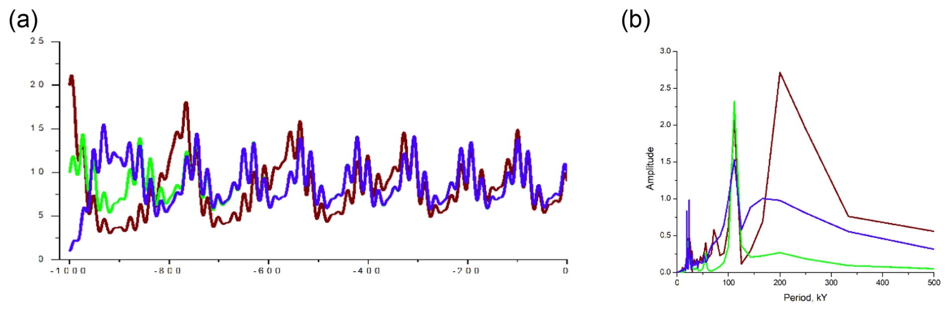
Figure 8 The dynamical system response to pure eccentricity-modulated precession, $F=\mathrm{0.7}\left[\sin \left(\frac{\mathrm{2}\mathit{\pi }t}{\mathrm{19}}\right)+\sin \left(\frac{\mathrm{2}\mathit{\pi }t}{\mathrm{23}}\right)\right]$, $\widehat{a}=\mathrm{0.0325}$. Here (a) the time series (kyr before present) of the area of glaciation in (10⁶ km²) and (b) corresponding spectral diagrams; brown is for $S\left(\mathrm{0}\right)=\mathrm{20}\times {\mathrm{10}}^{\mathrm{6}}$ km²; green is for $S\left(\mathrm{0}\right)=\mathrm{10}\times {\mathrm{10}}^{\mathrm{6}}$ km²; blue is for $S\left(\mathrm{0}\right)=\mathrm{1}\times {\mathrm{10}}^{\mathrm{6}}$ km².

Finding the exact functions Φ_M and Φ_P as well as precise values of power degrees μ and ν is outside of the scope of this article, and until this is done the laws (13) and (16) are qualitative statements that, nevertheless, allow us to answer the question raised about a decade ago (Crucifix, 2013): Why could ice ages be unpredictable? In this specific regard, the results are very eloquent: (a) when system's memory is short, the period of its response to astronomical forcing is fully defined by the ratio of the orbital forcing amplitude to the amplitude of the terrestrial mass influx, $\frac{\mathit{\epsilon }}{\widehat{a}}$, and by the V-number that is the ratio of terrestrial positive-to-negative feedbacks amplitudes (Eq. 6, Figs. 2 and 3, Verbitsky and Crucifix, 2020); (b) weaker (but not very weak) astronomical forcing (Figs. 4 and 5) or weaker terrestrial influx (Fig. 7) may make the memory longer, but, more importantly, they make the memory duration to become dependent on the initial conditions. This can in turn change the ice-age periodicity dramatically. The conglomerate C-number, emerging as a result of incomplete similarity property, is in the center of the process. Its critical dependence on poorly defined accumulation-minus-ablation mass balance as well as its dependence on initial values makes ice ages to be fundamentally difficult to predict.

4 The role of Obliquity and Eccentricity in a 100 kyr World – the attribution challenge

The role of the obliquity and eccentricity periods in the ∼100 kyr rhythmicity of the Late Pleistocene ice ages has been continuously debated. A systematic review of earlier works can be found in Saltzman (2002) and more recent efforts have been thoughtfully reviewed in, e.g., Huybers and Wunsch (2005), Tziperman et al. (2006), Huybers (2006, 2009, 2011), Crucifix (2012, 2013), Berger (2013), VCV18, Ganopolski (2024). There is no consensus here. For example Huybers (2009) proposes that “… When forced at a 40 kyr period the model chaotically transitions between small 40 kyr glacial cycles and larger 80 and 120 ky cycles which, on average, give the ∼100 kyr variability”; VCV18 argues in favor of the obliquity-period doubling; and Ganopolski (2024) declares that “… the obliquity component of orbital forcing … has nothing to do with the dominant 100 kyr periodicity of the glacial cycles of the late Quaternary”. In this section, being prompted by the scaling law we have just derived, we will investigate the role of orbital periods in appearance of ∼100 kyr periodicity.

Discovering the property of incomplete similarity in a system is always insightful. Simply speaking, the conglomerate similarity parameters tell us that a physical phenomenon may be produced by physically unsimilar processes. For example, our learning that the dynamical properties of the ice-climate system (3)–(5) are largely described by a conglomerate similarity parameter, the V-number, which is the ratio of amplitudes of positive and negative feedbacks led us to the attribution challenge – we demonstrated that major events of the past, like the middle-Pleistocene transition, could have been produced by multiple physically unsimilar scenarios. Some of these scenarios were based on the strengthening of positive feedbacks, and some scenarios described the middle-Pleistocene transition as the result of weakened negative feedbacks (Verbitsky, 2022).

The conglomerate similarity parameter, the C-number, that defines the memory-duration sensitivity to initial values, is the ratio of the timescale of vertical advection and the period of orbital forcing. It implies that though we have discovered this phenomenon using the obliquity periods, there is nothing unique about it. Therefore the response to the eccentricity-modulated precession should not be immune from the initial-value sensitivity either. Indeed, since the eccentricity period is longer than the obliquity period, it takes a consistently longer advection timescale to obtain the initial-value-sensitive memory. In Fig. 8, we present the dynamical system response to the pure eccentricity-modulated precession forcing, when ε_o=0, but ε_p=0.7 combined with $\widehat{a}=\mathrm{0.0325}$ km kyr⁻¹. It can be observed that the memory duration M and the dominant-period trajectories in this case are also sensitive to initial conditions.

Further, since the dominant-period trajectory of the system response to the astronomical forcing (16), for a given balance of positive and negative feedbacks (V=const), is also determined by the C-number, there should be initial values that would allow generating the “eccentricity” period P with the obliquity forcing T. Figure 7 may be a good example of such a response. It is pure obliquity forcing but the spectral diagram clearly shows the “eccentricity” pick without real eccentricity being involved.

Figure 9 is even more remarkable. It is, again, the same pure obliquity forcing and only initial conditions are different from Fig. 7: $S\left(\mathrm{0}\right)=\mathrm{12.0666}\times {\mathrm{10}}^{\mathrm{6}}$ km² instead of $S\left(\mathrm{0}\right)=\mathrm{20}\times {\mathrm{10}}^{\mathrm{6}}$ km². The time series show classical asymmetrical ice-age variability of dominant 100 kyr obliquity-forced period. Interestingly, the self-repeating pattern of the model time series is quite reminiscent, with Pearson correlation of 0.72, of the last 500 kyr of the LR04 data, including the interglacial of 400 kyr ago (marine isotopic stage 11) that is usually a challenge to reproduce. Most amazingly, no special efforts have been taken, i.e., none of the model parameters have been changed, in order to get this pattern, only the initial value has been adjusted, $S\left(\mathrm{0}\right)=\mathrm{12.0666}\times {\mathrm{10}}^{\mathrm{6}}$ km², four decimal digits being illustrative about model's sensitivity.

Thus, the ∼100 kyr periods in the observational time series could have been produced either

1. by the eccentricity modulated precession forcing in a short-memory system that is not sensitive to initial conditions due to the strong amplitude of the eccentricity modulated precession forcing (Fig. 1); or

2. by the eccentricity modulated precession forcing in a long-memory system that is sensitive to initial conditions due to a weakened amplitude of the eccentricity modulated precession forcing and weakened terrestrial mass influx, under favorable initial conditions (Fig. 8); or

3. by the obliquity forcing in a long-memory system that is sensitive to initial conditions due to a weakened terrestrial mass influx, under favorable initial conditions (Figs. 7 and 9).

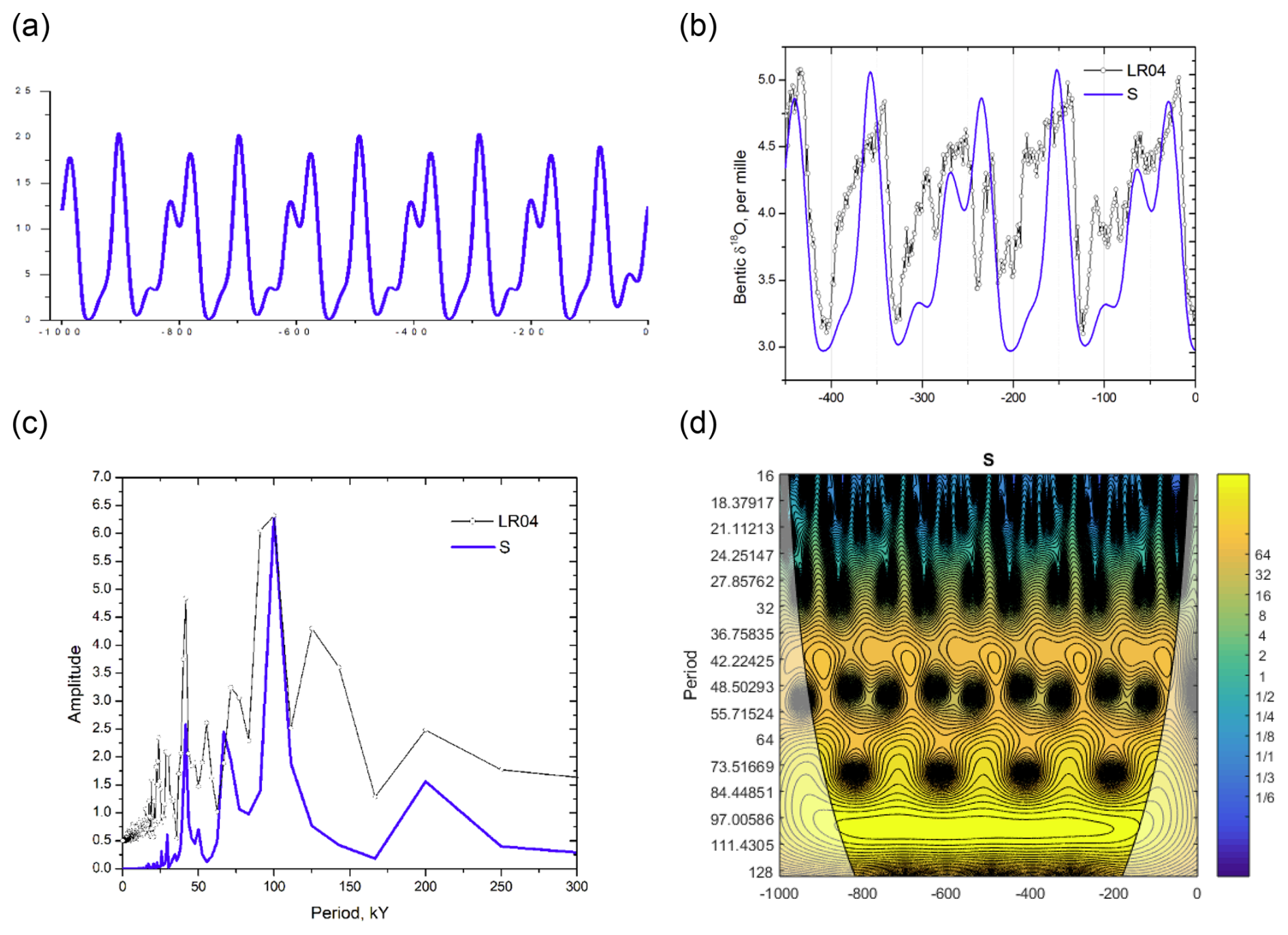
Figure 9 The dynamical system response to pure obliquity forcing, $F=\mathrm{1}\sin \left(\frac{\mathrm{2}\mathit{\pi }t}{\mathrm{41}}\right)$, $\widehat{a}=\mathrm{0.035}$. Here (a) is the time series (kyr before present) of the area of glaciation in (10⁶ km²); (b) last 500 kyr of the Lisiecki and Raymo (2005, “LR04” stack) benthic foraminifera δ¹⁸O data against the self-repeating pattern of the model time series; (c–d) are the spectral diagram and the evolution of the wavelet spectra for model glaciation area time series; all for $S\left(\mathrm{0}\right)=\mathrm{12.0666}\times {\mathrm{10}}^{\mathrm{6}}$ km².

Generally speaking, while our previous studies have highlighted multiple scenarios of the Eq. (6)-driven middle-Pleistocene transition (Verbitsky and Crucifix, 2020, Verbitsky, 2022), Eq. (16) opens an opportunity (some people would say a “Pandora box”) to envision even more scenarios. For example, we may suggest that the early-Pleistocene ice-climate system is the short-memory system that is, due to intensive terrestrial mass influx, evolves with 40 kyr obliquity driven periodicity according to Eq. (6). Figure 3 may serve as an illustration (since a response of the short-memory system is defined by the ratio of the orbital forcing amplitude to the amplitude of the terrestrial mass influx $\frac{\mathit{\epsilon }}{\widehat{a}}$, ε_o=0.5 of Fig. 3 is equivalent to doubled $\widehat{a})$. Further reduction of the terrestrial mass influx leads to the 80 kyr obliquity-period doubling (Eq. 6, Fig. 2). Additional reduction of the terrestrial mass influx and consequently longer vertical advection timescale leads to the long-memory initial-value-sensitive system that under favorable initial conditions produces still obliquity-driven 100 kyr periods (Fig. 9). This sequence of events would produce the middle-Pleistocene transition and the observed late Pleistocene dominant-period slope from 80 to 100 kyr.

Figure 10 The time series of Fig. 9 extended to 2 million years.

Obviously, this scenario is different from what we have invoked earlier to illustrate the dominant-period slope in the LR04 data, i.e., a combination of the initial-value-independent eccentricity period and the obliquity period evolving according to the law (16) with the initial conditions $S\left(\mathrm{0}\right)=\mathrm{1}\times {\mathrm{10}}^{\mathrm{6}}$ km² (Figs. 5 and 6). It is also different from multiple scenarios described by Verbitsky (2022). Moreover, there may be (most likely, there must be) an interplay between the V-number scenarios of Verbitsky (2022) and the C-number scenarios of this presentation. So far, in this study, we did not change model parameters involved in the V-number conglomerate. However, we should be mindful that vertical advection also affects the thickness of the ice-sheet basal boundary layer. Therefore, the parameter β that defines the intensity of basal sliding, i.e., intensity of the negative feedback, may change in concert with vertical advection.

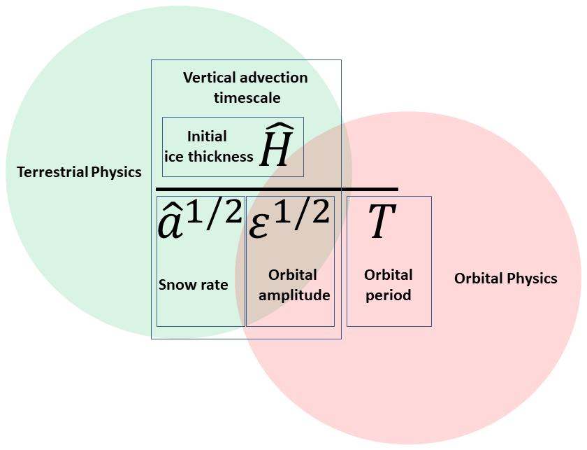
Figure 11 The C-number, i.e., $C=\frac{\widehat{H}}{{\widehat{a}}^{\mathrm{1}/\mathrm{2}}{\mathit{\epsilon }}^{\mathrm{1}/\mathrm{2}}T}$, as the ratio of the orbital-forcing period and orbitally modified vertical advection timescale of ice media.

This is the essence of the fundamental attribution challenge. We warned about it in the Introduction when we entertained a simple dynamical system (1), but it may be repeated here almost without changes: Any claim that nature is just like a model because that model has successfully reproduced a sample time series, should be taken cautiously unless our knowledge about mass balance and internal dynamics is unambiguous. As we already know, this is not the case.

5 Initial Value Problem versus Phase Locking. The Middle-Pleistocene Transition as a Delayed Phase Locking

For the last few decades, the ice-age-study community has been fascinated with reproducing ice-volume empirical data. A significant number of so called conceptual or phenomenological models have been introduced. Though most of these models have not been derived from the laws of physics, all of them reproduced the empirical data successfully. In a landmark work, Tziperman et al. (2006) established that a reasonable fit to empirical data can be achieved by phase locking of any non-linear oscillator to the Milankovitch forcing and therefore successful fit does not imply the correct physics.

Later, Verbitsky and Crucifix (2023) demonstrated that some of these phenomenological models may not have physical similarity with the nature. The “nature” of the study was the VCV18 model because it has not been postulated but instead it was derived from the scaled conservation equations of the non-Newtonian ice flow. The comparison was done in terms of the similarity parameters, one of them being the V-number. In some of the phenomenological models (e.g., van der Pol model in the form adopted by Crucifix, 2012), the V-number was much lower than in VCV18. It means that, in the phenomenological models, the intensity of negative feedbacks may be overstated. If this is indeed the case, this may be an explanation why these phenomenological models can effectively erase the memory of initial values and be quickly phase locked.

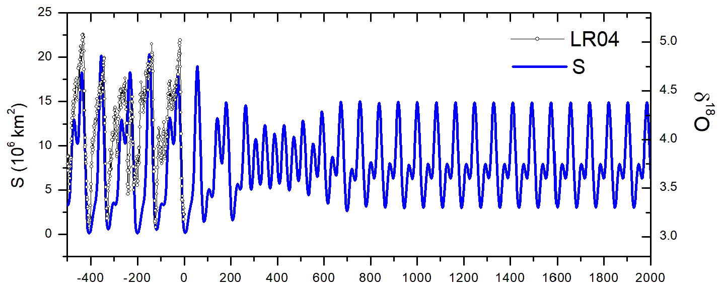
As we have already established, in the VCV18 model the memory of its initial conditions may be long. Therefore, this paper is about the climate system that cannot be “instantly” phase locked. Nevertheless, we demonstrated (i.e., Fig. 9), that to get a reasonable fit to the empirical data, the system does not need to be phase locked and the relaxation process may be very consistent with the empirical data under favorable initial conditions. This does not mean, however, that the phase locking is not real – in the long-memory system it may simply be significantly delayed. In Fig. 10, we extend Fig. 9 time series to 2 million years. It can be seen that in this case it takes more than a million years for VCV18 to be phase-locked.

Since we force our model with a pure obliquity forcing without a particular connection to the celestial timing, any part of Fig. 10 time series can be taking as a separate experiment with the initial values corresponding the starting point. With this caveat in mind, we may observe that the last 1.8 million years of this time series has a sharp dominant-periodicity transition from ∼40 to 80 kyr produced without any changes of parameters. This observation implies an intriguing hypothesis: The middle-Pleistocene transition may be a manifestation of the terrestrial long-memory, delayed phase locking response to the orbital forcing.

The abrupt periodicity transition from ∼100 kyr dominant periods to 40 kyr periods following the late Pleistocene ice ages in Fig. 10 is not less remarkable and provides an alternative to Talento and Ganopolski (2021) insight into the future ice ages that may include middle-Pleistocene-transition-like events.

We are now back to the question we first formulated in the Introduction: Does the terrestrial climate system, or more specifically, continental ice sheets, indeed have short memory of the initial values? If it is short, the phase locking is a viable mechanism to explain the late Pleistocene climate history. If it is long, the explanation may be in Figs. 9 and 10.

6 Discussion and conclusions

In this paper we describe a so far unrecognized physical phenomenon of the orbital forcing modifying the terrestrial physics in such a way that instead of erasing memory of the initial conditions this memory is extended and the initial values become major governing parameters. As it is evident from the structure of the C-similarity parameter (we illustrate it graphically in Fig. 11), the amplitude of the orbital forcing ε may change the timescale of ice vertical advection. Hence, the orbital forcing enables the sensitivity of the terrestrial system to the initial ice thickness$\widehat{H}$.

Thus, in our interpretation, the Milankovitch theory is very explicit:

1. The dynamics of large ice sheets is defined by the advection of mass and temperature;

2. The timescale of ice advection depends mostly on the surface total mass influx;

3. Because of the ice-climate system's nonlinearity, its response to the orbital forcing in terms of engagement of negative and positive feedbacks is not symmetrical. This may change the effective mass influx and the resultant advection timescale;

4. Specifically, an orbital forcing of relatively weak amplitude may make the ice-sheet advection timescale significantly longer. It means that the ice-climate system may remember its initial values through the entire Late Pleistocene, and for the same orbital forcing and for the same balance between terrestrial positive and negative feedbacks, the historical glacial rhythmicity could have been dominated either by the eccentricity period of ∼100 kyr, or by the doubled obliquity period of ∼80 kyr, or by a combination of both;

5. In fact, empirical records demonstrate that the dominant period of the Late Pleistocene ice ages evolved from ∼80 to ∼100 kyr rhythmicity. The quantitative similarity of this dominant-period trajectory and the one, made by the long-memory model, suggests that the records of the Late Pleistocene glacial rhythmicity could have been produced by an initial-value-dependent climate system, or, in other words, the slopes in empirical dominant-period trajectories are signatures of a long memory.

6. The scaling law of the dominant-period trajectory provides a theoretical insight into the discovered phenomenon. It reveals that this trajectory is dependent on a memory duration that is sensitive to initial conditions. The sensitivity of the memory duration to initial values emerges as the result of system's incomplete similarity in two similarity parameters colliding into one conglomerate similarity parameter that is the ratio of the orbitally modified advection timescale and the orbital period. The critical dependence of this similarity parameter on the poorly defined accumulation-minus-ablation mass balance as well as its dependence on initial values makes ice ages fundamentally difficult to predict. For the same reason, the disambiguation of paleo-records is extremely challenging.

7. The quasi-eccentricity periods produced by the long-memory system in response to pure obliquity forcing make a remarkable example of this challenge because in the time series they may be naively attributed to the eccentricity modulated precession forcing.

8. The long-memory relaxation time series may have dominant-periodicity transitions (e.g., from ∼40 to 80 kyr) produced without any changes of parameters. This observation implies that the middle-Pleistocene transition may be a manifestation of the terrestrial long-memory response to the orbital forcing.

Barry Saltzman has been advocating for dynamical paleoclimatology because the timing and amplitude of glacial variability are defined by poorly resolved ice-sheet mass balance, and the dynamical models, though they are not able to provide an unambiguous solution, can nevertheless expose the scope of the challenge. With this study, we want to expand this scope a bit more and to demonstrate, that since the timescale of vertical advection in ice sheets is defined by the same accumulation-minus-ablation mass balance, ice sheets' memory and periodicity can be sensitive to initial values. The implications of this sensitivity, as we discussed above, can be dramatic for our understanding of the past as well as for the future vision.

The ability to fit empirical time series is certainly tempting and self-gratifying. But we have to admit that simulating these times series with phenomenological models adds little to our understanding of nature simply because phenomenological models may not have physical similarity with nature or even with the comprehensive models they are designed to mimic (Verbitsky and Crucifix, 2023). Even when a model is based on a real physical phenomenon, the task of replicating empirical data may also be trivial as long as the model has a short memory of its initial values (Tziperman et al., 2006). Even reproducing empirical data with a short-memory three-dimensional or intermediate-complexity model does not give us more than evidence that this short-memory assumption is within the range of admissible parameters. Though such reconstructions of the historical data may be a natural first step in the studies, we nevertheless believe that the scientific community has been at this stage long enough and it is time to recognize the next challenge. We see this challenge as the ability to answer the following question: How long is the memory of the terrestrial climate system? Answering this question will support or reject the Milankovitch theory formulated here as an initial value problem.