Bayesian analysis of early warning signals using a time-dependent model

A tipping point is defined by the IPCC as a critical threshold beyond which a system reorganizes, often abruptly and/or irreversibly. Tipping points can be crossed solely by internal variation in the system or by approaching a bifurcation point where the current state loses stability, which forces the system to move to another stable state. It can be shown that before a bifurcation point is reached there are observable changes in the statistical properties of the state variable. These are known as early warning signals and include increased fluctuation and autocorrelation time. It is currently debated whether or not Dansgaard–Oeschger (DO) events, which are abrupt warmings of the North Atlantic region which occurred during the last glacial period, are preceded by early warning signals. To express the changes in statistical behavior we propose a model based on the well-known first-order autoregressive (AR) process, with modifications to the autocorrelation parameter such that it depends linearly on time. In order to estimate the time evolution of the autocorrelation parameter we adopt a hierarchical Bayesian modeling framework, from which Bayesian analysis can be performed using the methodology of integrated nested Laplace approximations. We then apply the model to segments of the oxygen isotope ratios from the Northern Greenland Ice Core Project record corresponding to 17 DO events. Statistically significant early warning signals are detected for a number of DO events, which suggests that such events could indeed exhibit signs of ongoing destabilization and may have been caused by approaching a bifurcation point. The methodology developed to perform the given early warning analyses can be applied more generally and is publicly available as the R package INLA.ews.

1 Introduction

If the state of a component of the climate system changes from one stable equilibrium to another, either by crossing some threshold in the form of a boundary of unstable fixed points separating two basins of attraction or by having the initial equilibrium destabilize, it is said to have crossed a tipping point. Components of the Earth system have experienced tipping points numerous times in the past, leading to abrupt transitions in the climate system. These transitions are well documented in paleoclimatic proxy records. Notably, in Greenland ice core records of oxygen isotope ratios (δ¹⁸O) and dust concentrations there is evidence that large and abrupt climatic transitions from Greenland stadial (GS) to Greenland interstadial (GI) conditions took place in the last glacial interval (110 000–12 000 years before 2000 CE, hereafter denoted yr b2k). These transitions are known as Dansgaard–Oeschger (DO) events (Dansgaard et al., 1984, 1993) and initialize climatic cycles where the temperature increases substantially, up to 16.5 °C for single events, over the course of a few decades. This is followed by a more gradual cooling, over centuries to millennia, returning to the GS state. A total of 17 DO events (Rasmussen et al., 2014) have been found for the past 60 kyr and they represent some of the most pronounced examples of abrupt transitions in past climate observed in paleoclimatic records.

It is widely accepted that such transitions are related to a change in the meridional overturning circulation (MOC) (Lynch-Stieglitz, 2017; Henry et al., 2016; Menviel et al., 2014, 2020; Bond et al., 1999), possibly caused by loss of sea ice in the North Atlantic. However, the physical mechanisms that caused these changes in the MOC and how they triggered DO events are less understood. Some studies have found that DO events exhibit a periodicity of 1470 years (Schulz, 2002), which has made some scientists suggest that the events have been triggered by changes in the Earth system caused by quasi-periodic changes in the solar forcing (Braun et al., 2005). Others suggest that the transitions have been triggered by random fluctuations in the Earth system, without any significant changes to the underlying system caused by external forcing (Ditlevsen et al., 2007). Treating the GS and GI states as stable equilibria in a dynamical system representing the Greenland climate, and studying the statistical behavior related to the stability of the system in the period preceding DO events, can help determine whether or not they are forced or random and thus possibly constrain the number of plausible physical causes that trigger the events.

Let a time-dependent state variable x(t), representing for example the δ¹⁸O ratio, vary over some potential V(x) with stochastic forcing corresponding to a white noise process dB(t), expressed as the derivative of a Brownian motion; then the stability of the system can be modeled using the stochastic differential equation:

$$\begin{array}{}\text{(1)}& \mathrm{d}x\left(t\right)=F\left(x\right(t\left)\right)\mathrm{d}t+\mathit{\sigma }\mathrm{d}B\left(t\right).\end{array}$$

One could interpret this equation as describing the motion of some particle in the presence of a potential V(x), with drift expressed by $F\left(x\right)=-V^{\prime }\left(x\right)$ and a diffusion term σdB(t) describing the noise that acts on the particle. Points where $\mathrm{d}x\left(t\right)/\mathrm{d}t=\mathrm{0}$ are fixed points. These are stable if a small perturbation of the state variable near the fixed point decays in time and unstable otherwise. Figure 1a illustrates an example of a potential with two valleys corresponding to stable fixed points x₁ and x₃ that are separated by an unstable fixed point x₂. If a state variable near x₁ crosses x₂ into the basin of attraction of x₃ solely from perturbations caused by internal variation of the system, then the associated tipping point is said to be noise-induced. However, if the dynamics of the system depend on some slowly varying control parameter μ(t), then the equilibrium points may shift, vanish, or spawn as a function of μ(t). This means that an equilibrium state of a system can change over time and eventually be lost, making the system move to another equilibrium, as illustrated in Fig. 1a–c. Points in the control parameter space for which the qualitative behavior of a system changes, e.g., changes in stability or the number of fixed points, are called bifurcation points. Figure 1d illustrates these changes using a bifurcation diagram, where the stable fixed points x₁ (lower solid curve) and x₃ (upper solid curve) are separated by the unstable fixed points x₂ (middle dashed curve). Critical transitions caused by the control parameter crossing a bifurcation point are said to be bifurcation-induced tipping points.

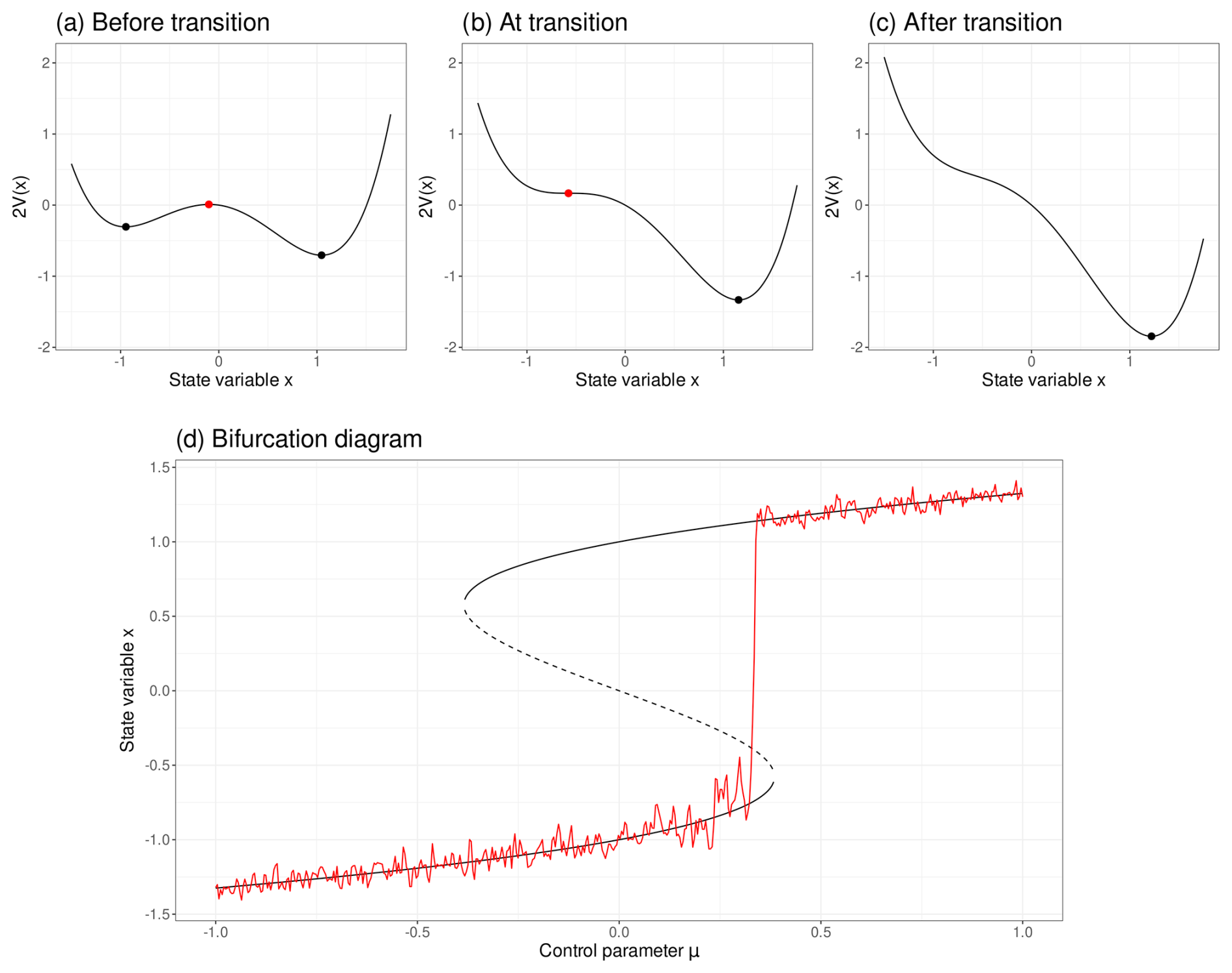
Figure 1 Panels (a)–(c) show the potential over the state variables before, at, and after the control parameter has reached the bifurcation point μ^*. Panel (a) shows the potential and fixed points x₁,x₂, and x₃ for some $\mathit{\mu }<{\mathit{\mu }}^{*}$, and panels (b)–(c) show the same for $\mathit{\mu }={\mathit{\mu }}^{*}$ and $\mathit{\mu }>{\mathit{\mu }}^{*}$, respectively. When the control parameter approaches the bifurcation point μ^*, the stability of the stable fixed point x₁ decreases and eventually collapses with x₂. In panel (b) they coincide as a single unstable saddle point, leaving x₃ as the only (stable) fixed point. (d) Bifurcation diagram describing a bifurcation-induced tipping point. The black curve represents the fixed points of the state variable x given the linearly changing control parameter $\mathit{\mu }\in (-\mathrm{1},\mathrm{1})$. The solid curves represent stable fixed points x₁ and x₃, and the dashed curve represents unstable fixed points x₂. The red line represents a simulated process. As the control parameter μ approaches the bifurcation point μ^* the stability of x₁ decreases, which is expressed by increased variance and autocorrelation in the simulated process, causing the system to cross the tipping point x₂ prematurely.

The nature of an equilibrium can be investigated by examining the linear approximation in its nearby domain. Linearizing Eq. (1) around some stable fixed point x_s yields

$$\begin{array}{}\text{(2)}& \mathrm{d}x\left(t\right)=-\mathit{\lambda }\left(x\right(t)-x_{\mathrm{s}})\mathrm{d}t+\mathit{\sigma }\mathrm{d}B\left(t\right),\end{array}$$

where $\mathit{\lambda }=-F^{\prime }\left(x_{\mathrm{s}}\right)$. This is known as the Langevin stochastic differential equation and has the solution

$$\begin{array}{}\text{(3)}& x\left(t\right)=x_{\mathrm{0}}+\underset{-\mathrm{\infty }}{\overset{t}{\int }}g(t-s)\mathrm{d}B\left(s\right),\end{array}$$

with Green's function,

$$\begin{array}{}\text{(4)}& g\left(t\right)=\left\{\begin{array}{ll}\exp (-\mathit{\lambda }t),& x\ge \mathrm{0}\\ \mathrm{0},& x<\mathrm{0}\end{array}\right..\end{array}$$

This solution forms an Ornstein–Uhlenbeck (OU) process with variance $\text{Var}\left(x_t\right)={\mathit{\sigma }}^{\mathrm{2}}/\left(\mathrm{2}\mathit{\lambda }\right)$. Under discretization this is a first-order autoregressive (AR) process,

$$\begin{array}{}\text{(5)}& x_t=\mathit{\varphi }{x}_{t-\mathrm{1}}+{\mathit{\epsilon }}_t,{\mathit{\epsilon }}_t\sim \mathcal{N}\left(\mathrm{0},{\displaystyle \frac{\mathrm{1}-{\mathit{\varphi }}^{\mathrm{2}}}{\mathrm{2}\mathit{\lambda }}}{\mathit{\sigma }}^{\mathrm{2}}\right),\end{array}$$

with the lag-one autocorrelation parameter $\mathit{\varphi }=\exp (-\mathit{\lambda }\mathrm{\Delta }t)$.

When the control parameter approaches a bifurcation point the restoring rate λ goes to zero and consequently the variance and autocorrelation of the state variable will increase, as can be observed in Fig. 1d. This phenomenon was first demonstrated by inspecting the power spectra of a simple physical model by Wiesenfeld (1985). The idea was later extended to a complex Earth system model by Held and Kleinen (2004) and first applied to real data by Dakos et al. (2008). These changes in statistical behavior are called early warning signals (EWSs) of the bifurcation point, or critical slowing down (Lenton et al., 2012; Dakos et al., 2008), and can be used as precursors to help determine whether or not a tipping point is imminent. EWSs are derived from the linearization of the system around its fixed points; however, even in cases where the system dynamic is far from its equilibrium the same changes in statistical behavior can be found with a delay (Ritchie and Sieber, 2016).

Recent studies have discovered that several components in the Earth system exhibit EWSs and are at risk of approaching or have already reached a tipping point. This includes the western Greenland ice sheets (Boers and Rypdal, 2021), the Atlantic meridional overturning circulation (Boers, 2021), and the Amazon rainforest (Boulton et al., 2022).

Analysis of EWSs for DO events in the Greenland ice core record has been conducted by others, e.g., Ditlevsen and Johnsen (2010), who estimated the variance and autocorrelation over a sliding window where the system was assumed to be driven by white noise. Under these assumptions they were unable to detect a statistical significant increase in EWSs, suggesting that DO events are noise-induced. However, using different model assumptions, Rypdal (2016) was able to detect statistically significant EWSs in an ensemble of DO events. This was achieved by analyzing individual frequency bands separately, using a fractional Gaussian noise (fGn) (Mandelbrot and Van Ness, 1968) model to describe the noise. These results were corroborated by Boers (2018), who applied a similar strategy to a higher resolved version of the Northern Greenland Ice Core Project (NGRIP) δ¹⁸O dataset (Andersen et al., 2004; Gkinis et al., 2014).

Most approaches for detecting EWSs in the current literature require estimation of statistical properties such as variance and autocorrelation in a sliding window. Consequently, this requires a choice on the length of the window. Using a small window will allow the momentary state to be better depicted, but there will be fewer points used in the estimation and hence accuracy will suffer. On the other hand, if a larger window is used the estimated statistics will be more accurate but less representative of the momentary state as it represents an average over a larger timescale. The optimal choice of window length should ideally represent a good trade-off between accuracy and ability to represent momentary evolution, but this can be hard to determine in practice. In this paper we circumvent this issue and present a model-based approach where such a compromise is not required. By assuming that the autocorrelation parameter is time-dependent, following a specific linear structure, it is possible to formulate this into a hierarchical Bayesian model for which well-known computational frameworks can be applied. A Bayesian approach has the additional benefit of providing uncertainty estimates in the form of posterior distributions.

The paper is structured as follows. A description of the data used in this paper is included in Sect. 2. Section 3 details our methodology, including how we treat time dependence, how to formulate our model as a hierarchical Bayesian model, and how to perform statistical inference efficiently. Results are presented in Sect. 4 where our framework is applied first to simulated data, then to Dansgaard–Oeschger events observed in the δ¹⁸O data from the NGRIP record. Our results are compared with those obtained by Ditlevsen and Johnsen (2010), Rypdal (2016), and Boers (2018). Further discussion and conclusions are provided in Sect. 5.

2 NGRIP ice core data

The δ¹⁸O ratios are frequently used in paleoscience as proxies for temperature at the time of precipitation (Johnsen et al., 1992, 2001; Dansgaard et al., 1993; Andersen et al., 2004), where higher ratios signal colder climates and, conversely, warmer climates tend to result in lower ratios. We employ the δ¹⁸O proxy record from the Northern Greenland Ice Core Project (NGRIP) (North Greenland Ice Core Project members, 2004; Gkinis et al., 2014; Ruth et al., 2003). There are currently two different versions of the NGRIP/GICC05 data at different resolutions. We will apply our methodology to the higher-resolution record, which is sampled every 5 cm in depth. The NGRIP δ¹⁸O proxy record is defined on a temporal axis given by the Greenland Ice Core Chronology 2005 (GICC05) (Vinther et al., 2006; Rasmussen et al., 2006; Andersen et al., 2006; Svensson et al., 2008) which thus pairs the δ¹⁸O measurements with a corresponding age, stretching back to 60 kyr b2k. We use segments of the δ¹⁸O record corresponding to Greenland stadial phases preceding DO onsets, as given by Table 2 of Rasmussen et al. (2014). The data used in this paper can be downloaded from https://www.iceandclimate.nbi.ku.dk/data/ (last access: 11 April 2025).

3 Methodology

During critical slowing down stationarity can no longer be assumed as we expect both the autocorrelation and variance to increase. For an AR(1) process $\mathit{x}=(x_{\mathrm{1}},\mathrm{\dots },x_n{)}^{\top }$ sampled at times $t_{\mathrm{1}},\mathrm{\dots },t_n$, we assume that the increase in autocorrelation can be expressed by representing the lag-one autocorrelation parameter as a linear function of time:

$$\begin{array}{}\text{(6)}& \mathit{\varphi }\left(t\right)=a+bt,\mathrm{0}\le t\le \mathrm{1},\end{array}$$

where a and b are two unknown parameters. The time-dependent AR(1) process is expressed by the difference equation given in Eq. (5) and the joint vector of variables $\mathit{x}=(x_{\mathrm{1}},\mathrm{\dots },x_n{)}^{\top }$ forms a multivariate Gaussian process,

$$\begin{array}{}\text{(7)}& \mathit{x}\sim \mathcal{N}(\mathbf{0}\mathbf{,}\mathbf{\Sigma }),\end{array}$$

where the covariance matrix is given by

$$\begin{array}{}\text{(8)}& {\mathrm{\Sigma }}_{ij}=\text{Cov}(x_i,x_j),\end{array}$$

and we assume that

$$\begin{array}{}\text{(9)}& \text{Var}\left(x_{\mathrm{1}}\right)={\displaystyle \frac{\mathrm{1}-{\mathit{\varphi }}^{\mathrm{2}}}{\mathrm{2}\mathit{\lambda }}}{\mathit{\sigma }}^{\mathrm{2}}.\end{array}$$

Since the covariance matrix is always dense for $\mathit{\varphi }\in (\mathrm{0},\mathrm{1})$ it is computationally beneficial to instead work with the inverse covariance matrix, also known as the precision matrix $\mathbf{Q}={\mathbf{\Sigma }}^{-\mathrm{1}}$. For consistency we hereafter use precision,

$$\begin{array}{}\text{(10)}& \mathit{\kappa }={\displaystyle \frac{\mathrm{2}\mathit{\lambda }}{(\mathrm{1}-{\mathit{\varphi }}^{\mathrm{2}}){\mathit{\sigma }}^{\mathrm{2}}}},\end{array}$$

instead of the variance as the unknown parameter of interest and denote κ(t_k)=2κλ(t_k) for $t_k=t_{\mathrm{2}},\mathrm{\dots },t_n$.

It can be shown that for a time-dependent AR(1) process the precision matrix is sparse and equal to

$$\begin{array}{}\text{(11)}& \mathbf{Q}=\left(\begin{array}{ccccc}\left(\mathit{\kappa }+\mathit{\kappa }\left(t_{\mathrm{2}}\right)\mathit{\varphi }(t_{\mathrm{2}}{)}^{\mathrm{2}}\right)& -\mathit{\kappa }\left(t_{\mathrm{2}}\right)\mathit{\varphi }\left(t_{\mathrm{2}}\right)& & & \\ -\mathit{\kappa }\left(t_{\mathrm{2}}\right)\mathit{\varphi }\left(t_{\mathrm{2}}\right)& \left(\mathit{\kappa }\left(t_{\mathrm{2}}\right)+\mathit{\kappa }\left(t_{\mathrm{3}}\right)\mathit{\varphi }(t_{\mathrm{3}}{)}^{\mathrm{2}}\right)& -\mathit{\kappa }\left(t_{\mathrm{3}}\right)\mathit{\varphi }\left(t_{\mathrm{3}}\right)& & \\ & \mathrm{\ddots }& \mathrm{\ddots }& \mathrm{\ddots }\\ & -\mathit{\kappa }\left(t_{n-\mathrm{1}}\right)\mathit{\varphi }\left(t_{n-\mathrm{1}}\right)& \left(\mathit{\kappa }\left(t_{n-\mathrm{1}}\right)+\mathit{\kappa }\left(t_n\right)\mathit{\varphi }(t_n{)}^{\mathrm{2}}\right)& -\mathit{\kappa }\left(t_n\right)\mathit{\varphi }\left(t_n\right)\\ & & -\mathit{\kappa }\left(t_n\right)\mathit{\varphi }\left(t_n\right)& \mathit{\kappa }\left(t_n\right)\end{array}\right).\end{array}$$

To allow for non-constant time steps $\mathrm{\Delta }{t}_k=t_k-t_{k-\mathrm{1}}$ we define

$$\begin{array}{}\text{(12)}& \mathit{\varphi }\left(t_k\right)=e^{-\mathit{\lambda }\left(t_k\right)\mathrm{\Delta }{t}_k/c},\end{array}$$

where

$$\begin{array}{}\text{(13)}& \mathit{\lambda }\left(t_k\right)=-\log (a+b{t}_k),\end{array}$$

$c={\sum }_{k=\mathrm{2}}^n\mathrm{\Delta }{t}_k/(n-\mathrm{1})$, and t_k has been rescaled such that $t_k\in (\mathrm{0},\mathrm{1})$. This modification guarantees that ϕ(t)⟶1 as Δt_k⟶0 and ϕ(t)⟶0 as Δt_k⟶∞. It also ensures that ϕ(t₁)=a and $\mathit{\varphi }\left(t_n\right)=a+b$, which makes the interpretability of the parameters easier.

Gaussian processes with sparse precision matrices are known as Gaussian Markov random fields, and there is a wealth of efficient algorithms for fast Bayesian inference; see, e.g., Rue and Held (2005) for a comprehensive discussion on this topic. These computationally efficient properties are not shared by the fractional Gaussian noise for which both the covariance matrix and the precision matrix are dense. This means that essential matrix operations such as computing the Cholesky decomposition will have a computational cost of 𝒪(n³) floating point operations (flops), as opposed to 𝒪(n) flops for the AR(1) process. Inference might still be possible to achieve in a reasonable amount of time if the size of the dataset remains sufficiently small. For larger datasets, however, both time and memory consumption may become an issue.

In fitting the model to data it is beneficial that the model parameters are defined on an unconstrained parameter space. We therefore introduce a suitable parameterization for the model parameters. For the precision κ we take the logarithm, θ_κ=log κ, and for a and b we use variations of the logistic transformation. Our reasoning is as follows. Assuming the lag-one autocorrelation parameter is defined on the interval (0,1), and since $t\in [\mathrm{0},\mathrm{1}]$, then the slope must be constrained by

$$\begin{array}{}\text{(14)}& \left|b\right|<\mathrm{1}.\end{array}$$

An unconstrained parameterization for b thus reads

$$\begin{array}{}\text{(15)}& \begin{array}{rl}& {\mathit{\theta }}_b=\log \left({\displaystyle \frac{\mathrm{1}+b}{\mathrm{1}-b}}\right)⟺b=-\mathrm{1}+{\displaystyle \frac{\mathrm{2}}{\mathrm{1}+\exp (-{\mathit{\theta }}_b)}},\\ & {\mathit{\theta }}_b\in (-\mathrm{\infty },\mathrm{\infty }).\end{array}\end{array}$$

The parameter space for a depends on the current state of b,

$$\begin{array}{}\text{(16)}& \mathrm{0}<a+bt<\mathrm{1}⟺-bt<a<\mathrm{1}-bt.\end{array}$$

Let

$$\begin{array}{}\text{(17)}& a_{\text{lower}}=-min(b,\mathrm{0})\text{ and }{a}_{\text{upper}}=\mathrm{1}-max(b,\mathrm{0}),\end{array}$$

and then an unconstrained parameterization for a is given by

$$\begin{array}{}\text{(18)}& \begin{array}{rl}& {\mathit{\theta }}_a=\log \left({\displaystyle \frac{a-a_{\text{lower}}}{a_{\text{upper}}-a}}\right)⟺a=a_{\text{lower}}+{\displaystyle \frac{a_{\text{upper}}-a_{\text{lower}}}{\mathrm{1}+\exp (-{\mathit{\theta }}_a)}},\\ & {\mathit{\theta }}_a\in (-\mathrm{\infty },\mathrm{\infty }).\end{array}\end{array}$$

3.1 Bayesian inference

Bayesian analysis presents a powerful framework for estimating model parameters that provides uncertainty quantification and allows us to incorporate prior knowledge about the parameters. These benefits are both very valuable in making informed decisions regarding climate action. In the Bayesian paradigm the model parameters $\mathit{\theta }=(\mathit{\kappa },b,a)$ are treated as stochastic variables for which prior knowledge is expressed using a predefined distribution π(θ). These are updated by new information expressed by the likelihood function of the observations $\mathit{x}=(x_{\mathrm{1}},\mathrm{\dots },x_n)$, which is a Gaussian distribution here,

$$\begin{array}{}\text{(19)}& \mathit{\pi }(\mathit{x}\mid \mathit{\theta })=\mathcal{N}\left(\mathbf{0},\mathbf{Q}(\mathit{\theta }{)}^{-\mathrm{1}}\right),\end{array}$$

with precision matrix Q(θ) as given by Eq. (11). The updated belief is expressed by the posterior distribution π(θ∣x), which is obtained using Bayes' rule,

$$\begin{array}{}\text{(20)}& \mathit{\pi }(\mathit{\theta }\mid \mathit{x})={\displaystyle \frac{\mathit{\pi }(\mathit{x}\mid \mathit{\theta })\mathit{\pi }\left(\mathit{\theta }\right)}{\mathit{\pi }\left(\mathit{x}\right)}},\end{array}$$

where the model evidence π(x) is a normalizing constant with respect to θ.

Prior selection is an essential part of any Bayesian analysis and presents a great strength of the Bayesian framework by allowing prior knowledge to be incorporated into models. Since we do not incorporate prior knowledge in this paper, and we wish to maintain objectivity, we will adopt vague prior distributions. These are distributions with large variances that express minimal information about the parameters and allow inference to be primarily driven by the data, as opposed to more informative priors which can guide the posterior to reflect prior knowledge or assumptions. Since the parameter a depends on the value of another parameter b we assign a conditional prior, π(a∣b), such that the joint prior is expressed by

$$\begin{array}{}\text{(21)}& \mathit{\pi }(\mathit{\kappa },b,a)=\mathit{\pi }\left(\mathit{\kappa }\right)\mathit{\pi }\left(b\right)\mathit{\pi }(a\mid b).\end{array}$$

Specifically, all analyses performed in this paper assume the same set of priors, unless otherwise specified. κ is assigned a gamma distribution with shape 1 and rate 0.1. b is assigned a uniform prior on $(-\mathrm{1},\mathrm{1})$ and a∣b is assigned a uniform prior on (a_lower,a_upper).

The main goal of this paper is to detect whether or not an early warning signal can be observed in the data. We are therefore primarily interested in the marginal posterior distribution of the slope parameter b,

$$\begin{array}{}\text{(22)}& \mathit{\pi }(b\mid \mathit{x})=\int \mathit{\pi }(\mathit{\theta }\mid \mathit{x})\text{d}\mathit{\kappa }\text{d}a.\end{array}$$

Typically, marginal posterior distributions can be evaluated using Markov chain Monte Carlo approaches (Robert and Casella, 2004), but these are very often time-consuming and could potentially be sensitive to convergence issues. However, since our model is Gaussian with a sparse precision matrix we instead use the computationally superior alternative of integrated nested Laplace approximation (INLA) (Rue et al., 2009), which is available as an R package at http://www.r-inla.org (last access: 11 April 2025).

To make the methodology more accessible we have released the code associated with this model as an R package titled INLA.ews, which can be downloaded at http://www.github.com/eirikmn/INLA.ews (last access: 11 April 2025). A demonstration of this package can be found in Appendix A, and a detailed description of its features can be found in its accompanying documentation.

3.2 Incorporating forcing

Climate components may also be affected by forcing, which can be measured alongside the climate variable of interest. How the observed component responds to such forcing will be influenced by time dependence. In this subsection we adopt a similar strategy to Myrvoll-Nilsen et al. (2020) with changes to the Green's function to allow for time dependence and non-constant time steps.

Let F(t) denote the known forcing component such that

$$\begin{array}{}\text{(23)}& \mathrm{d}x\left(t\right)=-\mathit{\lambda }x\left(t\right)+F\left(t\right)\mathrm{d}t+\mathrm{d}B\left(t\right).\end{array}$$

As shown in Gardiner (2009), the model can then be expressed as the sum of two components,

$$\begin{array}{}\text{(24)}& x\left(t\right)=\mathit{\nu }\left(t\right)+\mathit{\xi }\left(t\right),\end{array}$$

where ξ(t) is a time-dependent OU process and the forcing response is given by

$$\begin{array}{}\text{(25)}& \mathit{\nu }\left(t\right)={\displaystyle \frac{\mathrm{1}}{\sqrt{\mathrm{2}\mathit{\lambda }\left(t\right){\mathit{\kappa }}_f}}}\underset{\mathrm{0}}{\overset{t}{\int }}{e}^{-\mathit{\lambda }\left(t\right)(t-s)}\left(F\left(s\right)+F_{\mathrm{0}}\right)\mathrm{d}s.\end{array}$$

Here, $\mathit{\lambda }\left(t\right)=-\log \left(\mathit{\varphi }\right(t\left)\right)$ is the restoring rate, κ_f is an unknown scaling parameter, and F₀ is an unknown shift parameter. These parameters can be estimated using the same Bayesian framework as before, which can be computed with INLA.ews by specifying the forcing argument in the inla.ews function.

4 Results

4.1 Accuracy test on simulated data

To test the accuracy and robustness of the time-dependent AR(1) model we fit the model to a number of simulations. Specifically, we perform accuracy tests using a grid of $b\in [-\mathrm{0.8},\mathrm{0.8}]$ with increments of 0.1 and choose the parameter a corresponding to θ_a=0. For each b we draw n_r=1000 time series of length n=500 and n=1000 from the time-dependent AR(1) model. The model is fitted using R-INLA using priors specified in Sect. 3.1. To quantify the accuracy of the model we compare the posterior marginal mean of the slope $\widehat{b}=\text{E}\left(\mathit{\pi }\right(b\mid \mathit{x}\left)\right)$ to the true values b. We also compute the posterior probability of the slope being positive, denoted P(b>0). Ideally, we want $\widehat{b}$ to be as close to b as possible, and $P(b>\mathrm{0})>\mathrm{0.5}$ if b>0 and, conversely, $P(b>\mathrm{0})<\mathrm{0.5}$ if b<0. We also count the number of simulations where an EWS is detected using the threshold $P(b>\mathrm{0})\ge \mathrm{0.95}$. Since σ only scales the amplitude of the data without affecting the correlation structure we expect similar estimations for a and b regardless of the value of σ. This was confirmed by testing the model on simulations using both σ=1 and σ=10.

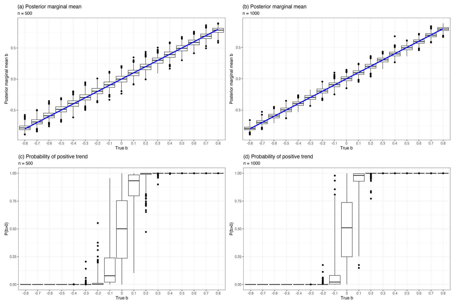
Figure 2 Box plots representing the results of the accuracy test for n_r=1000 simulated time series for $b\in [-\mathrm{0.8},\mathrm{0.8}]$. The boxes cover the interquartile range (IQR) between the 25 % and 75 % quantiles, and the whiskers represent an adjustment to the more common boundaries of 1.5 times the IQR to better describe skewed distributions. Points that fall outside the whiskers are classified as outliers and are also included in the plot. Panels (a) and (b) show box plots of the posterior marginal mean estimated by INLA for simulations of lengths n=500 and n=1000, respectively. The blue line shows the true b used in the simulation. Panels (c) and (d) show box plots of the estimated posterior probability of the slope being positive against different true values used for simulations of length n=500 and n=1000, respectively.

The results of the analysis are presented in Table 1 and displayed graphically as box plots in Fig. 2. Since the posterior distribution of b is skewed, especially when its absolute value approaches 1, ordinary box plots would classify a larger number of points as outliers. We instead use an adjusted box plot proposed by Hubert and Vandervieren (2008), which is better suited for skewed distributions. We obtain decent accuracy of the posterior marginal means $\widehat{b}$, with a small, but consistent, underestimation which decreases as n increases. In panels (c) and (d) of Fig. 2 we observe some variation in P(b>0) for small values of $\left|b\right|$ and less so for $\left|b\right|\ge \mathrm{0.2}$. This behavior also improves when n increases from 500 to 1000. By counting the number of simulations with detected EWSs for b≤0 using threshold $P(b>\mathrm{0})\ge \mathrm{0.95}$ we find 54 false positives for n=500 and 56 for n=1000. Out of 8000 simulations for b≥0.1 we find 669 false negatives for n=500 and 321 for n=1000, as reported in Table 1.

In order to assess how sensitive the model is to the choice of prior distribution we repeat the same simulation procedure with n=500 using different Gaussian priors on the parameters in their internal scaling,

$$\begin{array}{}\text{(26)}& \left(\log \right(\mathit{\kappa }),{\mathit{\theta }}_a,{\mathit{\theta }}_b)\sim \mathcal{N}\left(\mathbf{0},{\mathit{\sigma }}_{\mathit{\theta }}\mathbf{I}\right),\end{array}$$

where ${\mathit{\sigma }}_{\mathit{\theta }}\in \mathit{\{}\mathrm{0.1},\mathrm{1},\mathrm{10}\mathit{\}}$ and I is the identity matrix. The posterior marginal means and posterior probabilities P(b>0) for the different priors are compared to the default prior in Fig. 3. The results show that using the most informative prior, corresponding to σ_θ=0.1, will pull b too much towards the central value of b=0, resulting in worse estimates for b. This pull is also reflected in the posterior probability estimates, P(b>0), where this prior performs less well compared to the others, although the effect is less strong here. Counting the number of misclassifications, we find, for σ_θ equal to 0.1, 1 and 10, 4, 48, and 67 false positives our of 9000 simulations and 1255, 657, and 631 false negatives out of 8000 simulations, respectively. This is overall quite comparable to using the default priors, which found 54 false positives and 669 false negatives. Overall, we find the model to be quite robust to the choice of prior distributions as most of the priors perform very similarly in terms of the posterior marginal mean and posterior probabilities. However, we also find that using priors that are too informative could cause the model to be overly cautious, making it less able to detect EWSs.

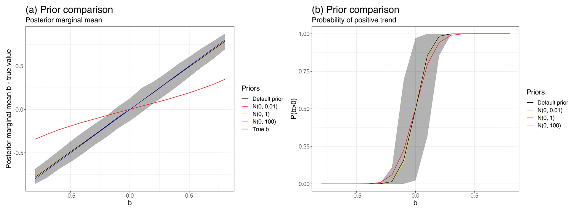
Figure 3 Prior sensitivity analysis on simulated data using the default priors (black) and Gaussian priors 𝒩(0,0.1²) (red), 𝒩(0,1) (orange), and 𝒩(0,10²) (yellow). Panel (a) shows the ensemble average of the posterior marginal mean estimates for b compared to the true value (blue), and panel (b) shows the ensemble average for the posterior probabilities P(b>0). The shaded gray area in both panels represents the ensemble spread of the estimates from the default prior using the 2.5 % and 97.5 % quantiles.

Table 1 Results from accuracy tests on n_r=1000 simulated time-dependent AR(1) series of length n for each b ranging from −0.8 to 0.8. The table includes the ensemble averages of the posterior marginal means $\widehat{b}$ and posterior probabilities of positive slope P(b>0) for each value of b and for time series' lengths of n=500 and n=1000. We also show the number of detected early warning signals using the threshold $P(b>\mathrm{0})\ge \mathrm{0.95}$.

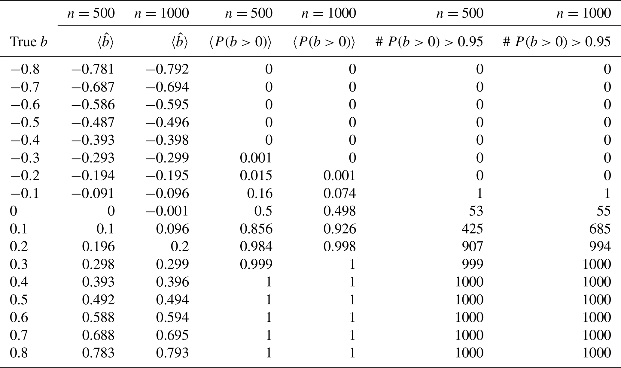
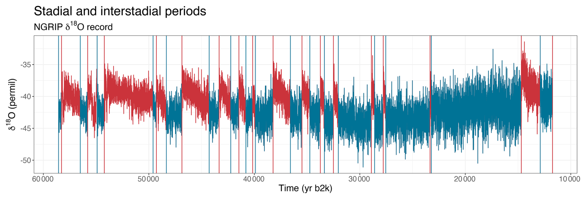
Figure 4 NGRIP δ¹⁸O proxy record. The time series used in our study are the parts of the curves drawn in turquoise, which are the cold stadial periods preceding the onsets of interstadial periods drawn in red. The red and turquoise vertical bars represent the start and end points of the interstadial periods, respectively.

4.2 DO events

We apply our time-dependent AR(1) model to the high-resolution NGRIP δ¹⁸O record, which is partitioned into stadial and interstadial periods as shown in Fig. 4. This version of the NGRIP record is sampled regularly every 5 cm step in depth but is non-constant in time. Having modified our model to allow for irregular time points we are able to use the raw NGRIP record without having to perform interpolation or other types of pre-processing, such as that of Boers (2018). This grants us a larger dataset for each event, which could significantly improve parameter estimation. Having implemented the model using INLA we are able to take advantage of this extra resolution while keeping computational time low.

Some of these datasets appear nonstationary and thus require trend estimation. Since there is no obvious choice of forcing we consider different alternatives for trend components which are then compared. The R-INLA framework allows us to very easily incorporate these trends into our model and estimates all model components simultaneously. First, we fit our model to the data without any additional trend, and then we assume a linear trend, followed by a second-order polynomial trend. Finally, we model the trend using a continuous second-order random walk (RW2) spline. More details on the comparison between the different trends are included in Appendix C, which also includes a plot of how well each trend fits the data.

Looking at the fits for each event we observe that most events can be fitted easily with a linear trend or even no trend, but a few events require nonlinearity. We choose the second-order polynomial trend as this gives a nice trade-off between flexibility and simplicity and appears to provide a decent fit for all events. The $\mathit{\varphi }\left(t\right)=a+bt$ evolutions for all events using second-order polynomial detrending are included in Fig. 5, and the posterior marginal distribution of the trend, π(b∣x), is included in Fig. 6.

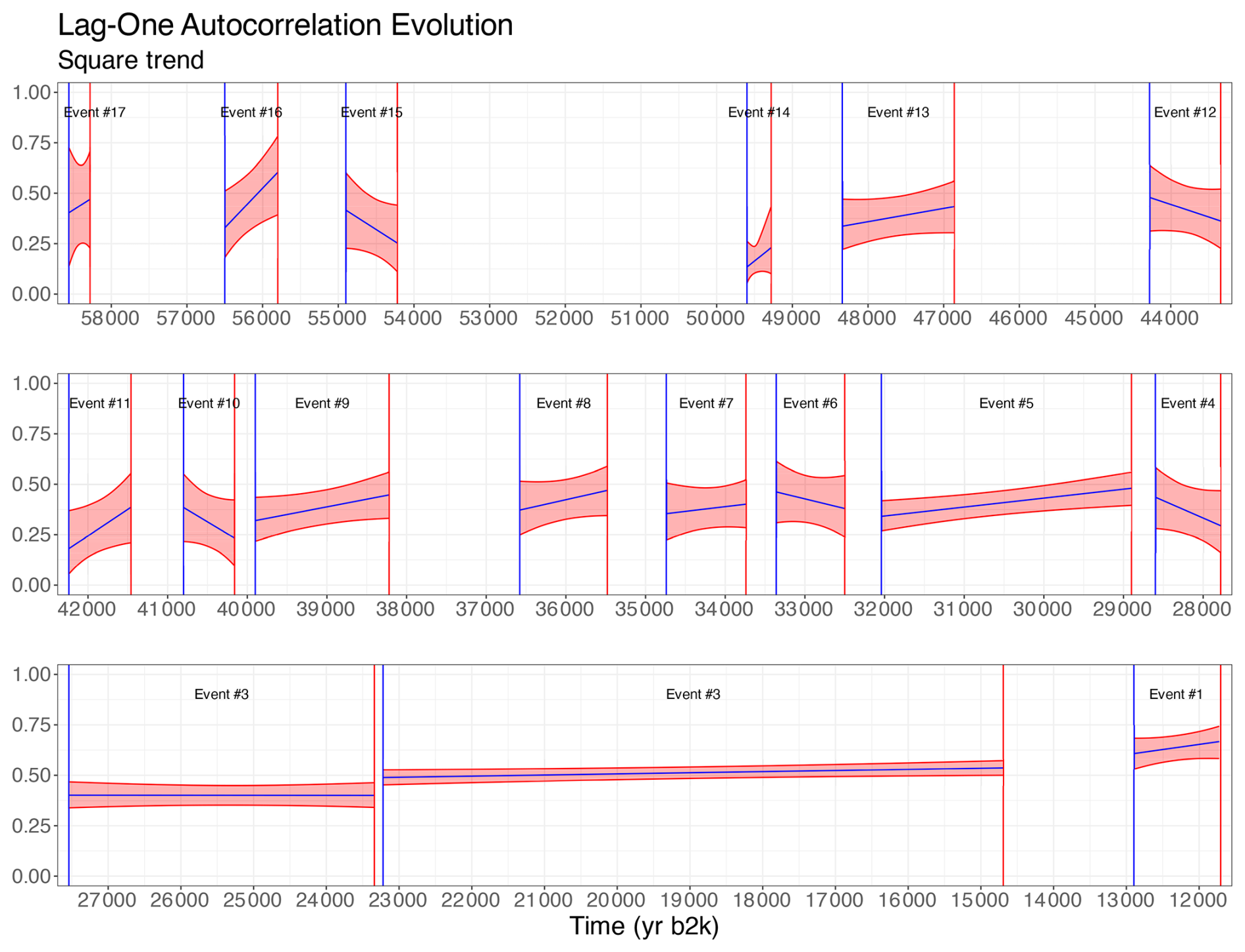
Figure 5 The evolution of the lag-one autocorrelation parameter a+bt for each of the 17 transitions analyzed in this paper. The blue lines represent the posterior marginal means of each Greenland stadial phase, and the red shaded areas represent the 95 % credible intervals (corresponding to the region between the 2.5 % and 97.5 % quantiles of the posterior distribution). The δ¹⁸O proxy measurements have been detrended using a second-order polynomial.

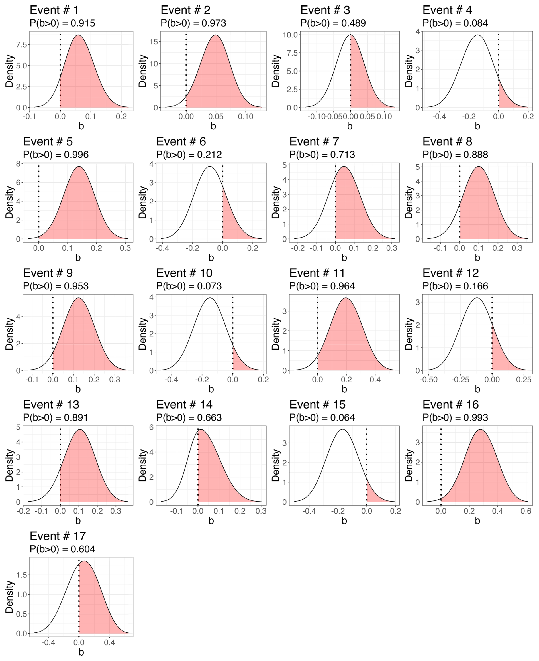
Figure 6 The marginal posterior distribution of the trend parameter b. The red dotted line represents b=0 and the red shaded area illustrates the density P(b>0). If the shaded area is larger than 0.95 we conclude that an EWS is detected.

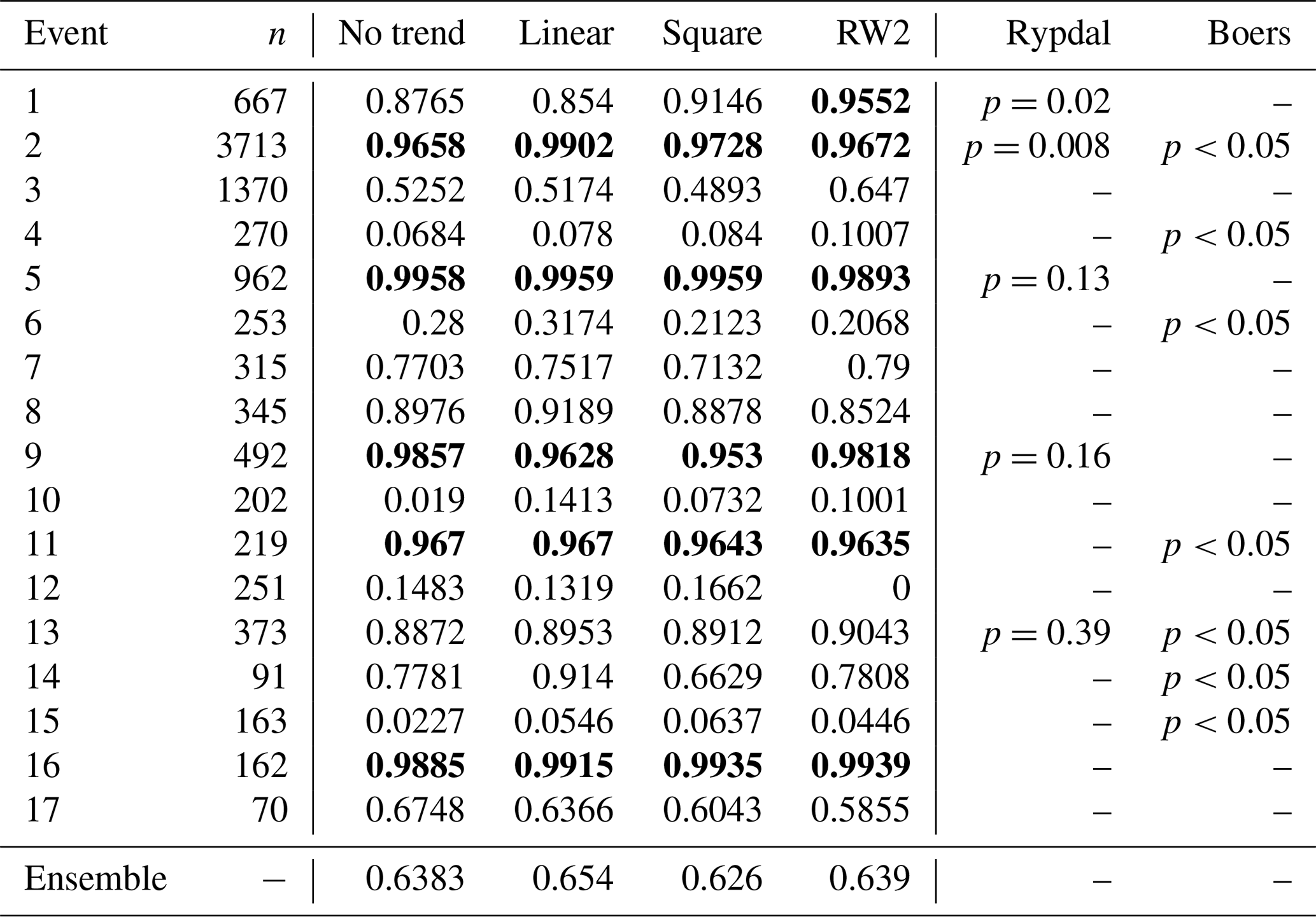
The models are fitted to the stadial periods preceding each of the 17 DO events, and the posterior probability of $\mathit{\varphi }\left(t\right)=a+bt$ being increasing, P(b>0), is compared for all events and trend assumptions. The results are included in Table 2. Using the conventional threshold of $P(b>\mathrm{0})\ge \mathrm{0.95}$ we are able to detect early warning signals in five events both without detrending and while using linear or second-order polynomial trends and six events using the continuous RW2 model as a trend. Averaging over the estimated P(b>0) for all events we are not able to conclude that early warning signals have been found over the ensemble of events for any detrending model.

Having found EWSs in multiple stadial periods preceding DO events therefore indicates that DO events can exhibit evidence of ongoing destabilization, unlike the conclusion formulated in Ditlevsen and Johnsen (2010). These differences in results can be explained by the use of both a higher-resolution dataset and a methodology not involving time windows.

However, given the absence of EWSs in the ensemble of events does not support the hypothesis that all DO events exhibit signs of ongoing destabilization, and hence one cannot exclude the possibility of some events being purely noise-induced and not approaching a bifurcation point. Our results do, however, suggest that some specific transitions have undergone destabilization, which is in line with the results of Rypdal (2016) and Boers (2018), wherein significant EWSs have also been found only for some specific events. Specifically, Table 2 shows that using a square detrending our results corroborate the EWS found for events 5 and 9 by Rypdal (2016) and the one found for event 11 by Boers (2018); our results also show an EWS for event 2, similarly to these two studies.

These studies use different versions of the NGRIP record from our study and their methodologies differ from ours.

Table 2 Table comparing the probability of positive slope P(b>0) for each event given posterior distributions obtained using the time-dependent AR(1) model on preceding subintervals of lengths n. We ran the model using different trends including no trend (except for the intercept), a linear effect, a second-order polynomial, and a second-order random walk spline. Events where the posterior probability of a positive slope exceeds 0.95 are highlighted in bold. Our results are also compared with the p values obtained from Rypdal (2016) and Boers (2018).

5 Conclusions

In this paper we introduce a Bayesian framework to analyze early warning signals in time series data. Specifically, we define a time-dependent AR(1) process where the lag-one autocorrelation parameter is assumed to increase linearly over time. The slope of this parameter indicates whether or not memory is increasing and thus if early warning signals are detected. Using a Bayesian approach we automatically obtain uncertainty quantification expressed by posterior distributions and allow prior knowledge to be utilized.

To detect early warning signals of DO events we have applied our model to interstadial periods of the raw 5 cm NGRIP water isotope record. This record is sampled evenly in depth, but not in time, requiring us to make some necessary modifications to allow for non-constant time steps. Using the time-dependent AR(1) model we were unable to detect statistically significant EWSs for the ensemble of 17 DO events and only detected EWSs individually for six events using a second-order polynomial detrending. Unlike Ditlevsen and Johnsen (2010), we find evidence of EWSs in some events, corroborating Rypdal (2016) and Boers (2018). We were, however, unable to conclude that DO events are individually or generally bifurcation-induced. To better compare with other studies, we would have liked to employ a long-range-dependent process such as the fGn. However, this task is more difficult than for the AR(1) process, as necessary modifications have to be made to the model. Moreover, this would also require working with non-sparse precision matrices, which are far more computationally demanding. We did attempt to implement the time-dependent fGn model presented by Ryvkina (2015), but we were unable to ensure sufficient stability. This is, however, a very interesting topic for future work.

Currently, our model can only fit an AR(1) process where the lag-one autocorrelation parameter is expressed as a linear function of time, which is not realistic. Although this is sufficient for detecting whether or not there are EWSs expressed by a linear trend, our model is unable to perform predictions or give an indication of when the tipping point could be reached. More advanced functions for the evolution of the lag-one autocorrelation parameter should be possible but would have to be implemented. One possible extension would be to include a break point such that the memory is constant for all steps before this point and starts increasing or decreasing afterwards. A simple implementation and discussion of this are included in Appendix D. Another extension would be to formulate a model where the memory parameter follows a polynomial $\mathit{\varphi }\left(t\right)=a+b{t}^c$, where the exponent term c>0 is an additional hyperparameter. This would perhaps help give an indication of the rate at which the autocorrelation has increased. However, when adding more parameters one needs to be careful to avoid overfitting.

The ability to update prior beliefs in light of new evidence presents a great benefit of a Bayesian approach, and it presents an intuitive framework for iteratively updating the posterior distribution as new data become available by using the posterior distribution from previous analyses as the prior distribution in the analysis. This is of great relevance for monitoring climatic systems suspected of approaching a tipping point.

To make the methodology more accessible we have released the code associated with this model as an R package titled INLA.ews. This package performs all analysis and includes functions to plot and print key results from the analysis very easily. Although this paper focuses on the detection of EWSs in DO events observed in Greenland ice core records, our methodology is general and the INLA.ews package should be applicable to tipping points observed in other proxy records as well. We have also implemented the option of including forcing, for which the package will estimate the necessary parameters and compute the resulting forcing response. The package is demonstrated on simulated data in Appendix A.

Appendix A: Demonstration of the INLA.ews package

We demonstrate the INLA.ews package on simulated forced data with non-equidistant time steps. The time steps t_k are obtained by adding Gaussian noise such that ${\stackrel{\mathrm{̃}}{t}}_k=k+{\mathit{\xi }}_k$ and normalized $t_k=({\stackrel{\mathrm{̃}}{t}}_k-{\stackrel{\mathrm{̃}}{t}}_{\mathrm{0}})/({\stackrel{\mathrm{̃}}{t}}_n-{\stackrel{\mathrm{̃}}{t}}_{\mathrm{0}})$ such that t₀=0 and t_n=1. We assume a time-dependent AR(1) process of length n=1000 for the observations sampled at times ${\stackrel{\mathrm{̃}}{t}}_{\mathrm{1}},\mathrm{\dots },{\stackrel{\mathrm{̃}}{t}}_n$. The AR(1) process has a scale parameter κ=0.04 and time-dependent lag-one autocorrelation $\mathit{\varphi }\left(t\right)=a+b{t}_k$ given by a=0.3 and b=0.2. We also include a forcing F(t), obtained by simulation from another AR(1) process with unit variance and the lag-one autocorrelation parameter $\stackrel{\mathrm{̃}}{\mathit{\varphi }}=\mathrm{0.95}$. The forcing response is approximated by

$$\begin{array}{}\text{(A1)}& \mathit{\nu }\left(t_k\right)={\displaystyle \frac{{\mathit{\sigma }}_f}{\sqrt{\mathrm{2}\mathit{\lambda }(t_k})}}\sum _{s=t_{\mathrm{0}}}^{t_k}{e}^{-\mathit{\lambda }\left(t_k\right)(t_k-t_{\mathrm{s}})}(F_{\mathrm{0}}+F(s\left)\right),\end{array}$$

with parameters set to σ_f=0.1 and F₀=0, and added to the simulated observations. We assign gamma(1,0.01) priors for the precision parameters κ and κ_f, uniform priors on b and a, and a Gaussian prior 𝒩(0,10²) on F₀. For INLA.ews, these priors must be transformed for the unconstrained parameterization $\mathit{\theta }=(\log \mathit{\kappa },{\mathit{\theta }}_b,{\mathit{\theta }}_a,\log {\mathit{\kappa }}_f,F_{\mathrm{0}})$ using the change-of-variable formula. The logarithm of the prior distributions is specified by creating a function as follows.

    my.log.prior <- function(theta) {
        lprior = dgamma(exp(theta[1]), shape=1, rate=0.1) + theta[1] + #kappa
            -theta[2] -2*log(1+exp(-theta[2])) + #b
            -theta[3] -2*log(1+exp(-theta[3])) + #a
            dgamma(exp(theta[4]), shape=1, rate=0.1) + theta[4] + #kappa_f
            dnorm(theta[5], sd=10, log=TRUE) #F0
    return(lprior)
  }

It is then passed into inla.ews using the log.prior argument. The AR(1) model and forcing z sampled at time points time can be fitted to the data y with INLA using the inla.ews wrapper function.

results <- inla.ews(data=y, forcing=z,
log.prior=my.log.prior, timesteps=time)

The inla.ews function computes all posterior marginal distributions, computes summary statistics, formats the results, and returns all information as an inla.ews list object. Summary statistics and other important results can be extracted using the summary function.

> summary(results)

Call:
inla.ews(data = y, forcing = forcing, log.prior=my.log.prior, timesteps=time)

Time used:
   Running INLA Post processing           Total
       503.1737        151.8262        655.5909

Posterior marginal distributions for all parameters have been computed.

Summary statistics for using ar1 model (with forcing):
           mean     sd 0.025quant 0.5quant 0.975quant
a        0.3065 0.0546     0.1974   0.3072     0.4148
b        0.1929 0.0615     0.0524   0.2018     0.2878
sigma    7.0249 0.4522     6.3420   6.9522     8.0780
sigma_f  0.1000 0.0096     0.0862   0.0982     0.1229
F0      -0.0047 0.0223    -0.0514  -0.0034     0.0355

Memory evolution is sampled on an irregular grid.
Summary for first and last point in smoothed trajectory (a+b*time):
          mean     sd 0.025quant 0.5quant 0.975quant
phi0[1] 0.3065 0.0546     0.1974   0.3072     0.4148
phi0[n] 0.4980 0.0587     0.3667   0.5039     0.5945
Mean and 95% credible intervals for forced response have also been computed.

Probability of positive slope 'b' is 0.9954214

Marginal log-Likelihood: -3088.35

The results may be displayed graphically using the plot function.

> plot(results)

For this example the estimated memory evolution and forcing response are presented in Fig. A1. The estimated parameters are summarized in Table A1.

Table A1 Underlying values used for simulating the data, along with estimated posterior marginal means and 95 % credible intervals for all hyperparameters.

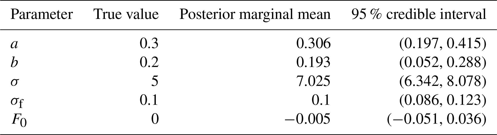
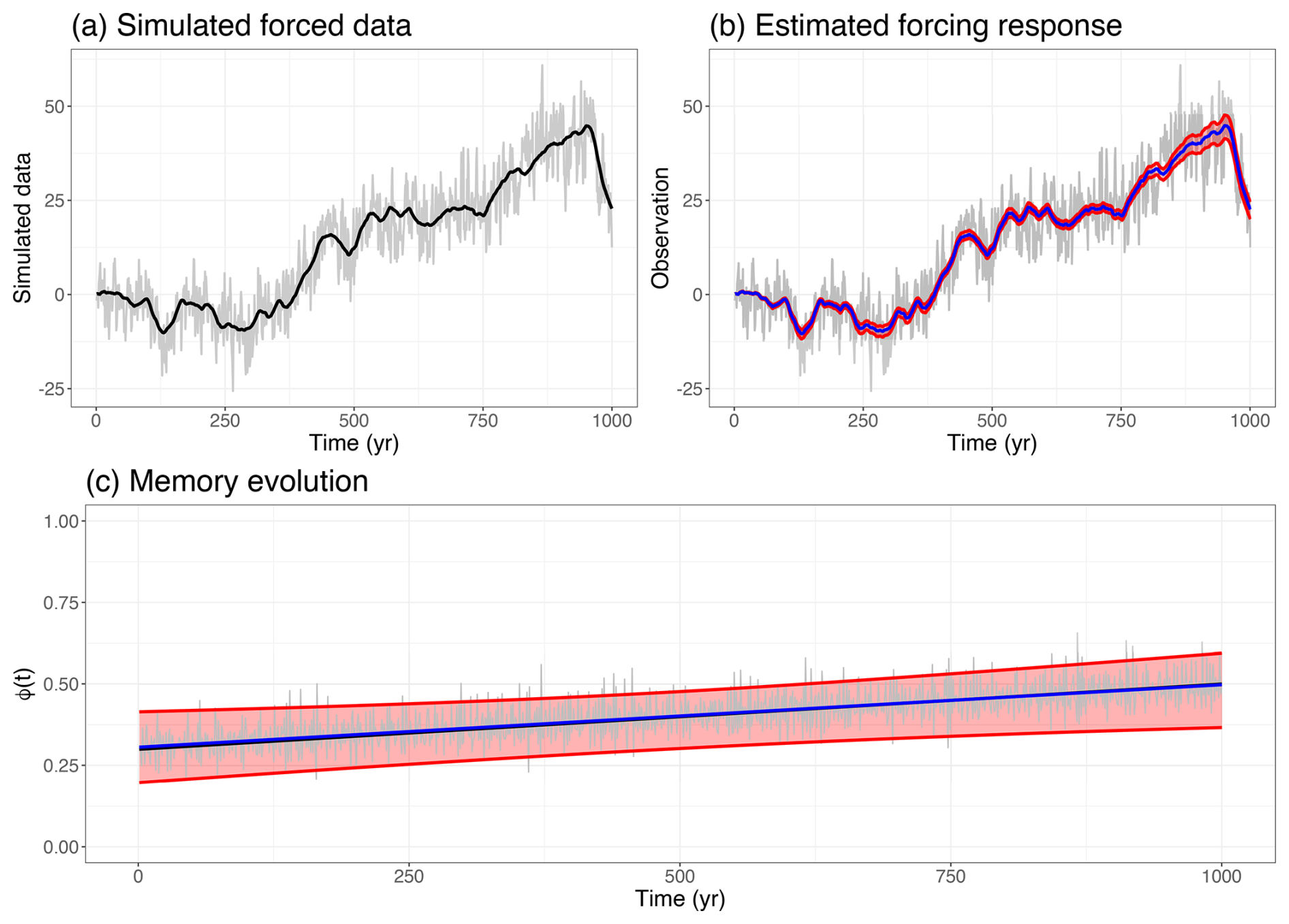
Figure A1 Panel (a) shows the simulated data (gray) where a simulated forcing response (black) has been added. Panel (b) shows the posterior marginal mean (blue) and 95% credible intervals (red) of the forcing response. Panel (c) shows the posterior marginal mean of the lag-one autocorrelation parameter of the simulated data (gray). The fluctuations are caused by being sampled at non-constant time steps. The posterior marginal mean of the smoother evolution of a+bt is included (blue), along with 95 % credible intervals (red) and the true values (white).

Combining forcing with irregular time steps requires more computationally intensive calculations within rgeneric, which increases the total computational time to around 10 min, compared to 10 s using any other model configuration. To reduce this we have implemented the model in cgeneric, which grants a substantial boost in speed. However, this requires pre-compiled C code using more simplistic priors for the parameters, which cannot be changed without recompiling the source code. Thus there could potentially be a small loss in accuracy of the fitted model at the cost of the improved speed. To use the cgeneric version of the model, set do.cgeneric=TRUE in the inla.ews function call.

Appendix B: Latent Gaussian model formulation

Section 3.1 defines our model within a Bayesian framework. However, in order for the model to be compatible with INLA we require some modifications such that it is expressed in terms of a latent Gaussian model. Latent Gaussian models represent a subset of hierarchical Bayesian models which are defined in three stages. First, the likelihood function is specified. The likelihood is then expressed using a latent field of unobserved Gaussian variables $\mathit{w}=(w_{\mathrm{1}},\mathrm{\dots },w_n)$ whose specification forms the second stage. These depend on a number of unknown hyperparameters. The final stage is to assign prior distributions to the hyperparameters.

Since our model is originally a two-stage model, a Gaussian likelihood that depends on some parameters without an intermediate latent field w, we reshape this into three stages by defining the former likelihood as the latent field w and the observations x to be the latent field with some additional negligible noise:

$$\begin{array}{}\text{(B1)}& \mathit{\pi }(\mathit{x}\mid \mathit{w},\mathit{\theta })=\prod _{i=\mathrm{1}}^n\mathcal{N}\left(w_i\left(\mathit{\theta }\right),{\mathit{\sigma }}_x^{\mathrm{2}}\right),\end{array}$$

where ${\mathit{\sigma }}_x^{\mathrm{2}}\approx \mathrm{0}$, essentially stating that x≈w. This trick does not change our model but creates a reformulation of the model into a latent Gaussian model where the latent field w is the prior of the mean of the likelihood.

The latent variables w follows a multivariate Gaussian process:

$$\begin{array}{}\text{(B2)}& \mathit{w}\mid \mathit{\theta }\sim \mathcal{N}\left(\mathit{\mu },\mathbf{Q}(\mathit{\theta }{)}^{-\mathrm{1}}\right),\end{array}$$

where the precision matrix Q is given by Eq. (11) and μ describes any potential trends as specified in the model. We will not discuss such trends here. When using INLA it is essential that the precision matrix is sparse in order to retain computational efficiency.

Since the Gaussian process now describes the latent variables instead of the likelihood, the parameters θ which govern w will now be called hyperparameters, since they are the parameters of a prior distribution. The final step of defining the latent Gaussian model is to assign prior distributions to the hyperparameters, but since INLA prefers to work with unconstrained variables these are specified through the parameterizations derived in Sect. 3:

$$\begin{array}{}\text{(B3)}& \mathit{\theta }\sim \mathit{\pi }\left(\log \mathit{\kappa }\right)\mathit{\pi }\left({\mathit{\theta }}_b\right)\mathit{\pi }({\mathit{\theta }}_a\mid {\mathit{\theta }}_b).\end{array}$$

Transforming priors chosen for $(\mathit{\kappa },b,a)$ to the corresponding priors chosen for $(\log \mathit{\kappa },{\mathit{\theta }}_b,{\mathit{\theta }}_a)$ can be done using the change-of-variable formula.

We want to estimate the marginal posterior distribution for all hyperparameters and latent variables. These are computed by evaluating the integrals

$$\begin{array}{}\text{(B4)}& {\displaystyle }\mathit{\pi }(w_i\mid \mathit{x})& {\displaystyle }=\int \mathit{\pi }(w_i\mid \mathit{\theta },\mathit{x})\mathit{\pi }(\mathit{\theta }\mid \mathit{x})d\mathit{\theta },\text{(B5)}& {\displaystyle }\mathit{\pi }({\mathit{\theta }}_j\mid \mathit{x})& {\displaystyle }=\int \mathit{\pi }(\mathit{\theta }\mid \mathit{x})d{\mathit{\theta }}_{-j}.\end{array}$$

Of these we are primarily concerned with the latter, since the latent field will very be similar to the observed values x since σ_x≈0. To compute these integrals INLA uses various numerical optimization techniques to obtain an appropriate approximation. Most important is the Laplace approximation (Tierney and Kadane, 1986), which is used to approximate the joint posterior distribution,

$$\begin{array}{}\text{(B6)}& \mathit{\pi }(\mathit{\theta }\mid \mathit{x})\approx {\left.{\displaystyle \frac{\mathit{\pi }(\mathit{w},\mathit{\theta },\mathit{x})}{{\mathit{\pi }}_G(\mathit{w}\mid \mathit{\theta },\mathit{x})}}\right|}_{\mathit{w}={\mathit{w}}^{*}\left(\mathit{\theta }\right)},\end{array}$$

where w^*(θ) is the mode of the latent field w(θ) and ${\mathit{\pi }}_G(\mathit{w}\mid \mathit{\theta },\mathit{x})$ is the Gaussian approximation of

$$\begin{array}{}\text{(B7)}& \mathit{\pi }(\mathit{w}\mid \mathit{\theta },\mathit{y})\propto \mathit{\pi }(\mathit{w}\mid \mathit{\theta })\mathit{\pi }(\mathit{x}\mid \mathit{w},\mathit{\theta }).\end{array}$$

The methodology is available as the open-source R package R-INLA, which can be downloaded at http://www.r-inla.org (last access: 11 April 2025).

Since there are no model components already implemented for R-INLA that meet our specifications we are required to implement the model components ourselves using the custom modeling framework of R-INLA called rgeneric. This adds more work and complexity in implementing our model and adds an additional barrier to further adoption of our methodology, which motivated us to create a more user-friendly R package titled INLA.ews, available at http://www.github.com/eirikmn/INLA.ews (last access: 11 April 2025).

Appendix C: Comparison of different detrending approaches

Since there is no clear choice of forcing for DO events, and not all data windows appear stationary, we assume that there is some unknown trend component reflected in the data. This trend needs to be managed or the estimates of other components will suffer. Often, this is done by first detrending the data, before the parameters of interest are estimated. This bears the risk that variation caused by the time-dependent noise component may be attributed to the trend, and it is therefore better to estimate both the trend and noise components simultaneously. This can be achieved using INLA, which supports many common model components. We perform the same analysis on the data windows preceding all 17 DO events using four different trend models.

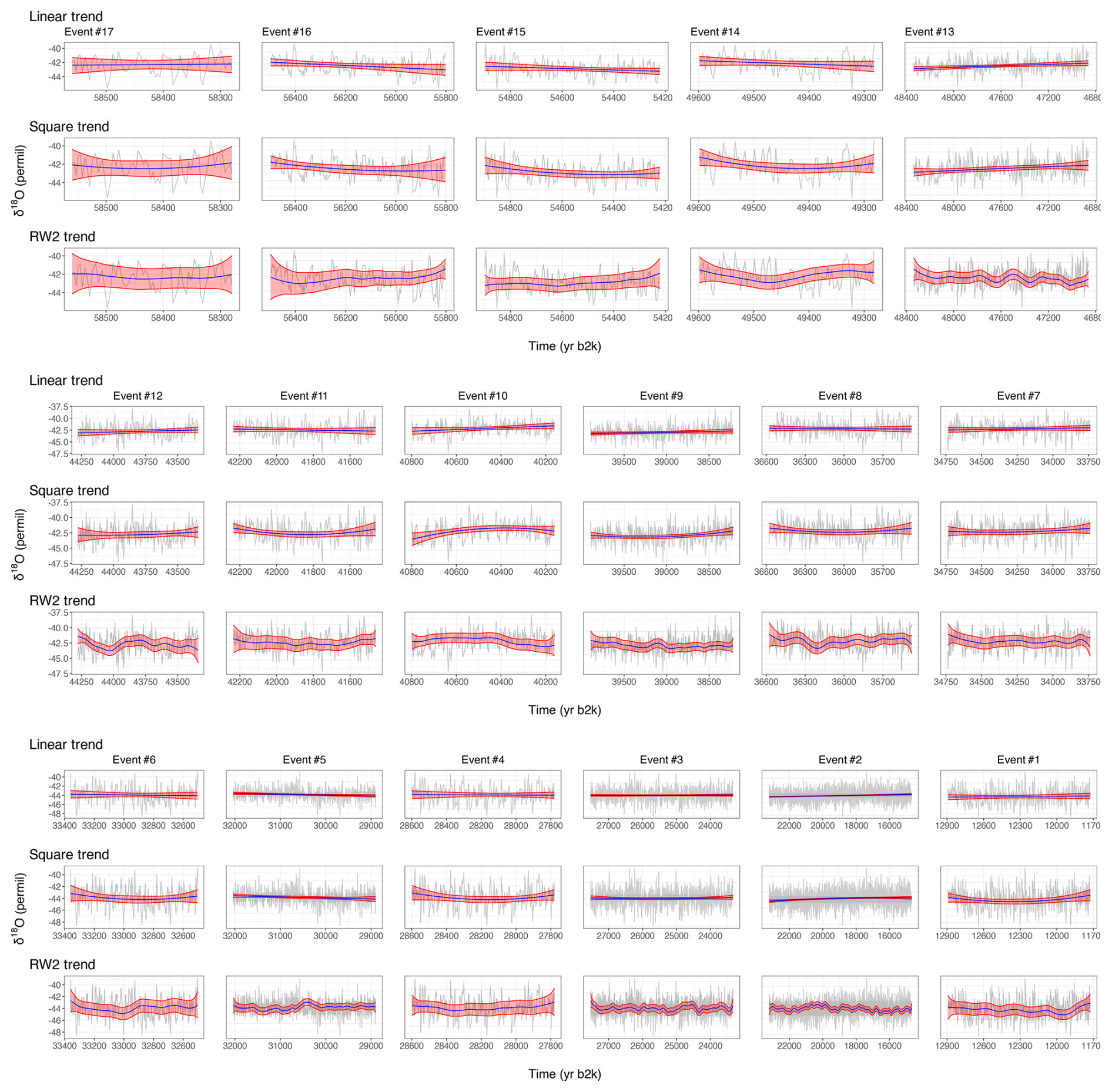
Figure C1 δ¹⁸O proxy data from the NGRIP record (gray), with Greenland stadial phases highlighted. The posterior marginal mean (blue) and 95 % credible intervals (red) of the fitted trends are included for each event.

• No trend: the data are explained using the time-dependent AR(1) noise component ε_t and an intercept β₀ only,

  $$\begin{array}{}\text{(C1)}& y_t\sim {\mathit{\beta }}_{\mathrm{0}}+{\mathit{\epsilon }}_t.\end{array}$$

  We only expect this to provide accurate results for stationary data windows. The results in this paper can be recreated using the INLA.ews package. Let y denote the δ¹⁸O ratios and time denote the GICC05 chronology, and then the model can be fitted by prompting the following.

  results = inla.ews(data=y, timesteps=time, formula = y ~ 1)  

  To omit the intercept term set the formula argument to formula = y ∼ -1 instead. The rgeneric model component corresponding to the time-dependent AR(1) noise is added automatically. To improve numerical convergence, we perform the analysis in iterations, restarting from the previously found optima with reduced step lengths. This can be specified using the stepsize argument in the inla.ews function. The length of this argument corresponds to the number of iterations. Here we used stepsizes = c(0.01, 0.005, 0.001).

• Linear trend: we incorporate an additional linear effect β₁ in the model,

  $$\begin{array}{}\text{(C2)}& y_t\sim {\mathit{\beta }}_{\mathrm{0}}+{\mathit{\beta }}_{\mathrm{1}}t+{\mathit{\epsilon }}_t.\end{array}$$

  This can capture linear increases but will not be able to model any nonlinearity in the data. This model can be fitted using the following.

  results = inla.ews(data=data.frame(y=y, trend1=time_norm),
           timesteps=time, formula = y ~ 1 + trend1)

  Here trend1 = time_norm is the covariate corresponding to the normalized time steps.

  time_norm = (time-time[1])/(time[n]-time[1])

• Second-order polynomial: we add another effect β₂ which allows nonlinearity to be described using a second-order polynomial trend,

  $$\begin{array}{}\text{(C3)}& y_t\sim {\mathit{\beta }}_{\mathrm{0}}+{\mathit{\beta }}_{\mathrm{1}}t+{\mathit{\beta }}_{\mathrm{2}}{t}^{\mathrm{2}}+{\mathit{\epsilon }}_t.\end{array}$$

  This model can be fitted using the following.

  results = inla.ews(data=data.frame(y=y,trend1=time_norm,trend2=time_norm^2),
           timesteps=time, formula = y ~ 1 + trend1 + trend2)

  Here trend2 specifies a linear response to the covariates defined as the square of the normalized GICC05 chronology trend2=time_norm**2.

• Continuous second-order random walk (CRW2): we use a random effect f(t) described by a continuous second-order random walk to describe the trend,

  $$\begin{array}{}\text{(C4)}& y_t\sim f\left(t\right)+{\mathit{\epsilon }}_t.\end{array}$$

  This is a continuous extension (Lindgren and Rue, 2008) of a stochastic spline model, which assumes that the second-order increments are independent Gaussian processes,

  $$\begin{array}{}\text{(C5)}& x_i-\mathrm{2}{x}_{i+\mathrm{1}}+x_{i+\mathrm{2}}\sim \mathcal{N}(\mathrm{0},{\mathit{\sigma }}_{\text{CRW2}}^{\mathrm{2}}).\end{array}$$

  This model is able to capture more general nonlinearities compared to the second-degree polynomial trend but makes the model less interpretable. Similarly as in R-INLA, the CRW2 model is specified using the following call.

  results = inla.ews(data=data.frame(y=y, idx=time,
           timesteps=time, formula = y ~ 1 + f(idx, model="crw2"))

  Here idx specifies the time steps of the continuous RW2 trend.

In Table 2 we present the estimated posterior probability of a positive trend, $P(b>\mathrm{0}\mid \mathit{y})$, compared to the corresponding p values by Rypdal (2016) and Boers (2018). We show the fitted trends for each data interval in Fig. C1. We observe that the models tend to agree, with some exceptions where the assumed trend is unable to capture the variation of the data. Although the RW2 trend is the most flexible model it appears to exhibit irregular fluctuation for several events. The second-order polynomial trend appears to be sufficiently flexible for all events and provides a much smoother and more interpretable fit.

Appendix D: Break point in memory evolution

Early warning signals are most easily detectable shortly before a bifurcation point. If the dataset covers a much larger period, for which most of it is stationary, it could be more difficult for the time-dependent AR(1) model to detect early warning signals if they are observable only for a much smaller subset of the data. To accommodate this one could add a break point, a point in time where the lag-one autocorrelation transitions from constant to linearly increasing.

Let t_bp denote a break point; the lag-one autocorrelation parameter is then defined by

$$\begin{array}{}\text{(D1)}& \mathit{\varphi }\left(t\right)=\left\{\begin{array}{ll}a,& t\le t_{\text{bp}}\\ a+\frac{b}{\mathrm{1}-t_{\text{bp}}}(t-t_{\text{bp}})& t>t_{\text{bp}}\end{array}\right..\end{array}$$

For stability, we constrain the break point parameter using the parameterization ${\mathit{\theta }}_{\text{bp}}=\mathrm{1}/(\mathrm{1}+\exp (-t_{\text{bp}}\left)\right)$ such that $t_{\text{bp}}\in (\mathrm{0},\mathrm{1})$. This model is demonstrated by fitting it to simulated data where t_bp=0.5. The results are presented visually in Fig. D1.

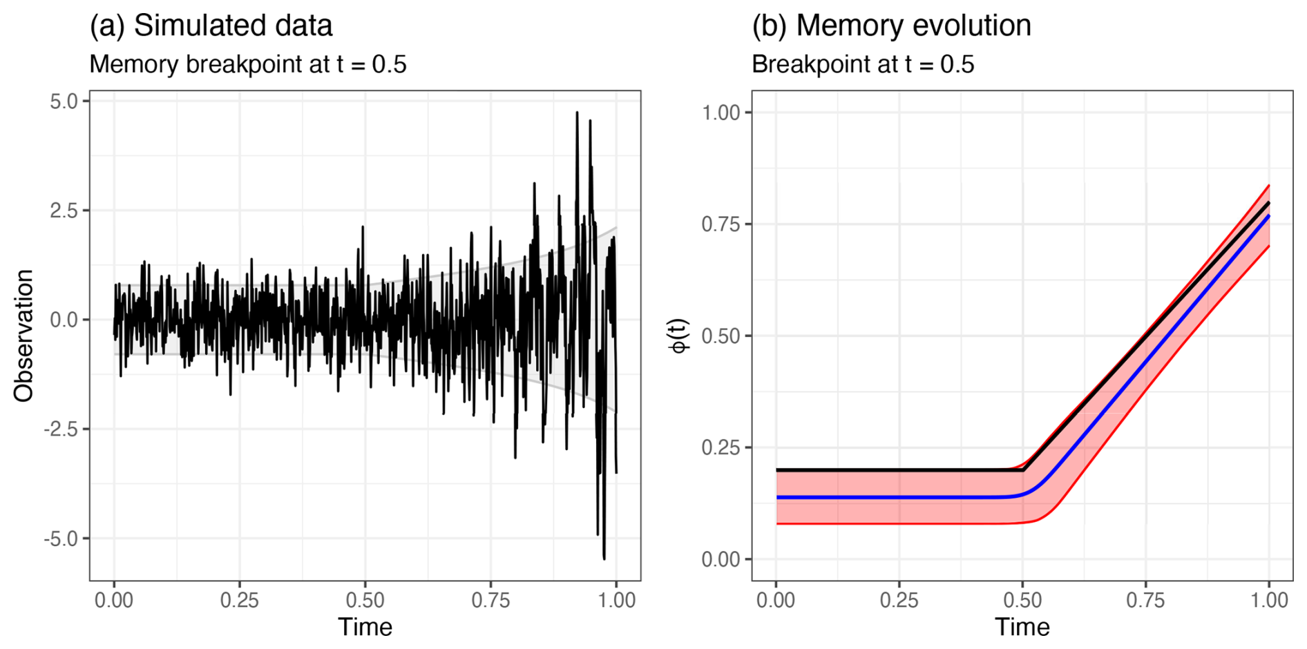
Figure D1 Panel (a) shows simulated data (black) with a break point located at t=0.5. The shaded gray area describes the standard deviation derived from using the true values. Panel (b) shows the posterior marginal means (blue) and 95 % credible intervals (red), with the true memory evolution (black).