Exploration of diverse solutions for the calibration of imperfect climate models

The calibration of Earth system model parameters is subject to data, time, and computational constraints. The high dimensionality of this calibration problem, combined with errors arising from model structural assumptions, makes it impossible to find model versions fully consistent with historical observations. Therefore, the potential for multiple plausible configurations presenting different trade-offs between skills in various variables and spatial regions remains usually untested. In this study, we lay out a formalism for making different assumptions about how ensemble variability in a perturbed physics ensemble relates to model error, proposing an empirical but practical solution for finding diverse near-optimal solutions. A meta-model is used to predict the outputs of a climate model reduced through principal component analysis. Then, a subset of input parameter values yielding results similar to a reference simulation is identified. We argue that the effective degrees of freedom in the model performance response to parameter input (the “parametric component”) are, in fact, relatively small, illustrating why manual calibration is often able to find near-optimal solutions. The results explore the potential for comparably performing parameter configurations that have different trade-offs in model errors. These model candidates can inform model development and could potentially lead to significantly different future climate evolution.

1 Introduction

General circulation models (GCMs) and Earth system models (ESMs) are the primary tools for making projections about the future state of the climate system. It is an important goal of climate science to continually improve these models and to better quantify their uncertainties (Balaji et al., 2022). Constraints on computational resources limit the ability to resolve small-scale mechanisms, and sub-grid parameterizations are used to represent processes such as atmospheric radiation, turbulence, or clouds. These parameterizations are based on numerous unconstrained parameters that introduce uncertainty in climate simulations. Therefore, climate models are subject to a challenging calibration (or “tuning”) problem. When used as tools for the projection of future climate trajectories, they cannot be calibrated directly on their performance. Instead, the assessment of performance and skill arises jointly from the confidence in the understood realism of physical parameterizations of relevant climatological processes, along with the fidelity of the model's representation of historical climate change. Practical approaches to model calibration are subject to data, time, and computational constraints.

For the simplest models (zero- or low-dimensional representations of the climate system), model simulations are sufficiently cheap, with sufficiently few degrees of freedom, so that Bayesian formalism can be fully applied to estimate model uncertainty (Ricciuto et al., 2008; Meinshausen et al., 2011; Bodman and Jones, 2016; Nauels et al., 2017; Dorheim et al., 2020). However, more complex models such as GCMs present a number of difficulties for objective calibration which have resulted in a status quo in which manual calibration remains the default approach (Mauritsen et al., 2012; Hourdin et al., 2017). Such approaches have not yet been operationally replaced by objective calibration approaches but leave large intractable uncertainties. In particular, the potential existence of comparably performing alternative configurations with significantly different future climate evolution (Ho et al., 2012; Hourdin et al., 2023) is rarely considered. Failing to explore alternative model configurations can result in model ensembles which may not adequately sample the projection uncertainty. For example, some of the CMIP6 model projections were “too hot” when compared with other lines of evidence, and using all of these models without statistical adjustment (in a simple “model democracy” approach) could lead to an overestimate of future temperature change (Hausfather et al., 2022).

Although manual calibration remains by far the most common practice, objective calibration methods have been developed and tested in climate models (Price et al., 2006; Nan et al., 2014; Sellar et al., 2019). Approaches to date with GCMs have mainly relied on perturbed parameter ensembles (PPEs) of simulations that allow an initial stochastic sample of the parametric response of the model. The construction of meta-models is then needed to emulate this parametric response and enhance the number of samples. The meta-models can be quadratic (Neelin et al., 2010), logistic regression (Bellprat et al., 2012), Gaussian process emulators (Salter and Williamson, 2016), or neural networks (Sanderson et al., 2008). Each of these meta-modeling approaches offers different advantages in terms of accuracy, flexibility, and speed (Lim and Zhai, 2017) but often requires prior assumptions on how smooth the parameter response surface might be and how noisy the samples themselves are. Such approaches allow for the definition of plausible or “not-ruled-out-yet” spaces when using a low-dimensional output space (such as global mean quantities; Bellprat et al., 2012; Williamson et al., 2015), potentially allowing for additional ensemble generations which sample in the not-ruled-out-yet space (Williamson et al., 2015). Emulators can be improved in promising sub-regions of the parameter space by running a new PPE in a reduced parameter space to increase the ensemble density (sometimes referred to as an “iterative refocusing” approach; Williamson et al., 2017). However, the choice of which region to initially focus on depends on advice from model developers and is itself subject to error in emulation. Finally, one of the strongest limitations when developing a GCM automatic tuning approach is the high computational cost of the PPE. Dunbar et al. (2021) rely on the calibrate–emulate–sample method to generate probability distributions of the parameters at a fraction of the computational cost usually required to obtain them, allowing for climate predictions with quantified parametric uncertainties.

Climate models produce high-dimensional output across space, time, and variable dimensions. Performance is often addressed by integrated output spanning these dimensions (Gleckler et al., 2008; Sanderson et al., 2017), and so calibration techniques must be able to represent spatial performance in order to be useful to development. In a low-dimensional space defined by global mean quantities, it is possible to find one model version which is consistent with observations (Williamson et al., 2015), but this is not true when considering the high dimensionality of climate model outputs. When considering an assessment of model error integrated over a large number of grid points and variables, structural trade-offs may arise between model outputs which cannot be simultaneously optimized by adjusting model parameters. For example, McNeall et al. (2016) found that land surface parameters which were optimal for the simulation of the representation of the Amazon rainforest fraction were not optimal for other regions. In another case, structural errors in an atmospheric model were found to increase significantly with the addition of variables to a spatial metric (Sanderson et al., 2008). As such, the potential structural error component is implicitly related to the dimensionality of the space in which the cost function is constructed. For example, Howland et al. (2022) demonstrated that the use of seasonally averaged climate statistics, rather than annually averaged ones, could narrow the uncertainty in the climate model predictions.

In order to reduce the complexity of the emulation problem and to preserve the covariance structure of the model output, it is common to reduce the dimensionality of the output through principal component analysis (PCA; e.g., Higdon et al., 2008; Wilkinson, 2010; Sexton et al., 2012). Notably, for some spatial applications, this dimensional reduction may be insufficient to resolve certain important climatological features such as extreme precipitation frequency (Jewson, 2020). This PCA representation, however, has some apparent drawbacks for optimization. An orthogonal space constructed from the dominant modes of variability in a PPE may not be able to describe some components of the spatial pattern of the model error (O'Lenic and Livezey, 1988). Salter et al. (2019) proposed an approach to the global optimization of a model with spatially complex output with a rotation of principal components such that model errors were describable on a reduced-dimensionality basis set by including some aspects of higher-order modes in the rotated, truncated basis set in order to better describe the error patterns of ensemble members. The method, however, makes some significant assumptions about the ability of a statistical model to predict the parametric response of high-order modes and does not allow an exploration of structural trade-offs between different variables, such as those found by McNeall et al. (2016).

In this study, we argue that considering a sub-set of plausible candidate calibrations sampling the diversity of model error spatial patterns can help us better understand the model biases. Such an approach could also help us to better understand model uncertainty in climate projections, as previous studies highlighted the possibility that several calibrations of a single climate model present very different future climates (Peatier et al., 2022; Hourdin et al., 2023). In this sense, we are not searching for an optimal parameter configuration but rather for model configurations which perform comparably to a reference model version. We lay out an alternative formalism which makes different assumptions about how the ensemble variability in a PPE relates to structural error and how it can thus inform model development. This formalism allows the empirical decomposition of the model error into one component, depending on the parameter values, and a component arising from structural inaccuracies. The approach, presented in Sect. 2, is used as a practical solution for finding diverse near-optimal solutions exploring key model error trade-offs. We start by illustrating the method using a simplified univariate case focusing on surface temperature errors (Sect. 3) before applying it to a more generalized multi-variate tuning case using five climatic fields (Sect. 4). Finally, we discuss and summarize the main results (Sect. 5).

2 Methods

2.1 Model and perturbed parameter ensemble (PPE)

The model used in this study is ARPEGE-Climate, the atmospheric component of the CNRM-CM6 climate model, referred to as f, the climate model. The reference configuration of this model will be referred to as CNRM-CM6-1 and has been tuned by the model developers for the CMIP6 exercise (Roehrig et al., 2020).

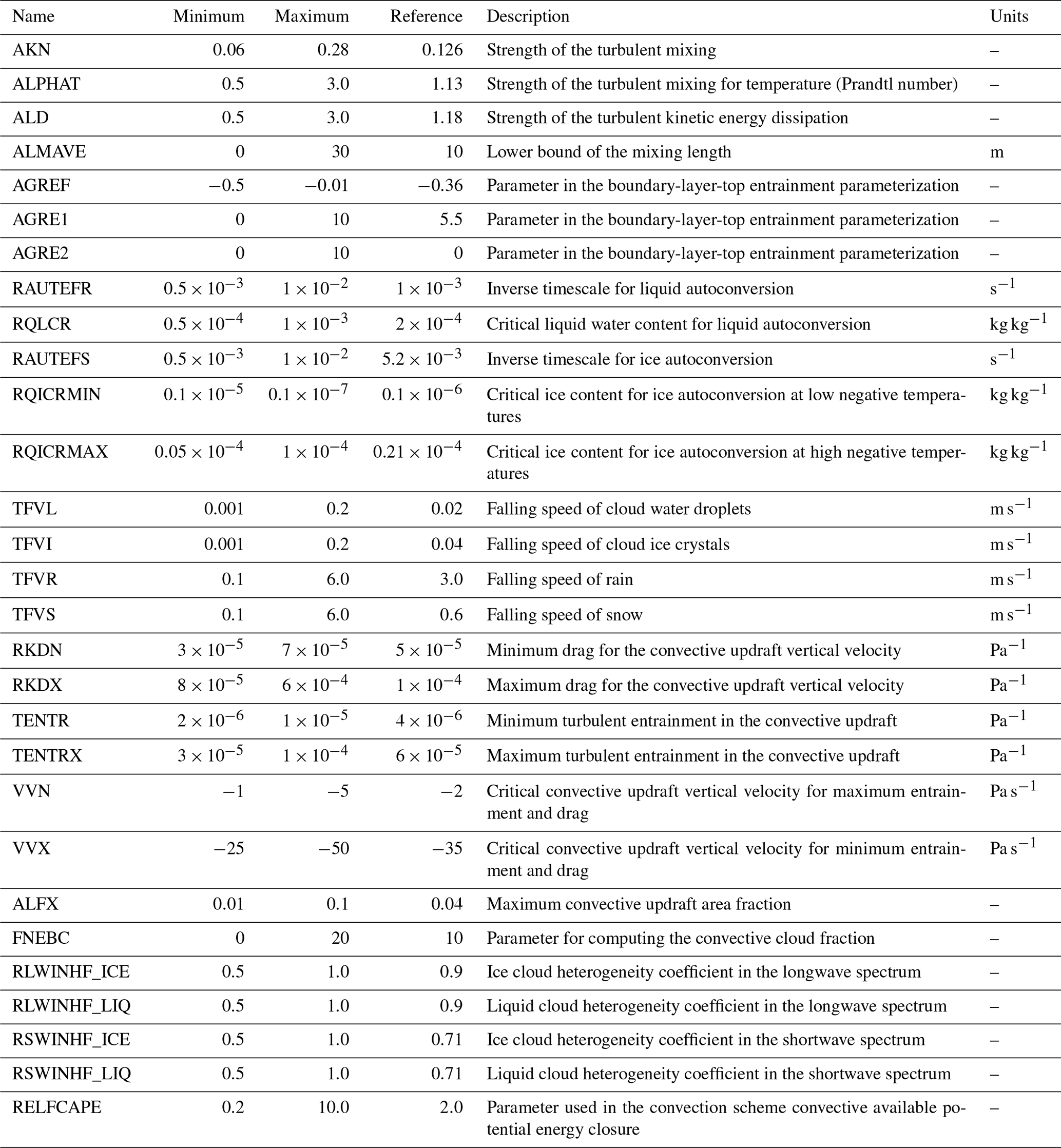
A PPE of this model is created, containing 102 AMIP simulations (Eyring et al., 2016) differing by their parameter values, representing the period 1979–1981 (3 years) with pre-specified sea surface temperatures (Peatier et al., 2022). In total, 30 model parameters (see Appendix A1) are perturbed with a Latin hypercube sampling (LHS) strategy based on a space-filling maximin design $\mathit{\theta }=({\mathit{\theta }}_{\mathrm{1}},\mathrm{\dots },{\mathit{\theta }}_n)$, producing a variety of simulated climate states $\mathbf{F}=\left(f\right({\mathit{\theta }}_{\mathrm{1}}),\mathrm{\dots },f({\mathit{\theta }}_n\left)\right)$, with n=102, and θ_i as a vector of 30 parameter values (Peatier et al., 2022). For the present study, we consider the annual means averaged over the whole 1979–1981 period as model outputs. We write the model output f(θ_i) as a vector of length l, such that F has dimension l×n, where n is the number of ensemble members (n=102), and l is the number of grid points (l = 32 768).

2.2 EOF analysis

In order to build emulators of a GCM's spatial climatology, the general practice is to reduce the dimensionality of the emulated response, and a common strategy is an EOF (empirical orthogonal function) analysis (Higdon et al., 2008; Wilkinson, 2010; Sexton et al., 2012; Salter et al., 2019) which produces n eigenvectors that can be used as basis vectors. Given n≪l, the reconstruction of F is exact and reduces the complexity of the emulator required.

Variability in F is explained in descending order of eigenvectors, such that a truncation to the first q modes yields a basis ${\mathrm{\Gamma }}_q=({\mathit{\gamma }}_{\mathrm{1}},\mathrm{\dots },{\mathit{\gamma }}_q)$ which produces an approximate reconstruction of the initial data, thus further reducing the scale of the emulation problem. Truncation length is often chosen such that a given fraction of ensemble variance (often 90 %–95 %) is preserved (Higdon et al., 2008; Chang et al., 2014), but some authors have argued that higher-order modes may need to be included to allow the resolution of optimal configurations (Salter et al., 2019). We discuss the choices of q in the first application (Sect. 3).

The EOF basis Γ_q is based on the centered ensemble (F−μ), with μ as the ensemble mean. As a result, each anomaly (f(θ_i)−μ) is associated with a coefficient c(θ_i) (or principal component, PC), such as

$$\begin{array}{}\text{(1)}& c\left({\mathit{\theta }}_i\right)=\left({\mathrm{\Gamma }}_q^T{\mathrm{\Gamma }}_q{)}^{-\mathrm{1}}{\mathrm{\Gamma }}_q^T\right(f\left({\mathit{\theta }}_i\right)-\mathit{\mu }).\end{array}$$

Given an orthogonal basis, the full spatial field of length l can be approximately reconstructed as a function of the q coefficients,

$$\begin{array}{}\text{(2)}& f\left({\mathit{\theta }}_i\right)-\mathit{\mu }={\mathrm{\Gamma }}_{q}c\left({\mathit{\theta }}_i\right)+r_f,\end{array}$$

with r_f as a residual that depends on the choice of q. Consider variable j (for example, the air surface temperature, as in the first application; Sect. 3.1), such that z_j is the observed field for the variable, and f_j(θ_i) is the model simulated field for that variable for a given parameter input θ_i. As for F, we can subtract the ensemble mean μ from the observation and project the anomaly of the observation (z_j−μ) (which is also the error in the ensemble mean μ) onto the basis Γ_q using Eq. (1):

$$\begin{array}{}\text{(3)}& z_i-\mathit{\mu }={\mathrm{\Gamma }}_q{c}_z+r_z,\end{array}$$

where r_z is a residual representing the part of the observation z_j that cannot be projected on the basis Γ_q. This residual r_z will, as for r_f, depend on the choice of q but will never (even when q=n) equal zero, as the basis Γ_q explains the maximum amount of variability in F but does not guarantee a full representation of the spatial pattern of the observation z_j (Salter et al., 2019).

2.3 Model error decomposition

The model error pattern of a given parameter sample, $E_j\left({\mathit{\theta }}_i\right)=z_j-f_j\left({\mathit{\theta }}_i\right)$, can be expressed in the basis Γ_q and becomes the sum of a term that depends on the vector of the parameter θ_i (here called a parametric component) and a term unsolvable in the basis Γ_q (here called non-parametric component):

$$\begin{array}{}\text{(4)}& {\displaystyle }{E}_j\left({\mathit{\theta }}_i\right){\displaystyle }=\underset{\mathrm{parametric}}{\underbrace{{\mathrm{\Gamma }}_q[c_z-c(\mathit{\theta }\left)\right]}}+\underset{\text{non-parametric}}{\underbrace{r_z-r_f}}.\end{array}$$

We could consider a skill score defined by the mean square error (MSE) of the spatial error pattern E_j(θ_i):

$$\begin{array}{}\text{(5)}& {\displaystyle }{e}_j\left({\mathit{\theta }}_i\right)& {\displaystyle }={\displaystyle \frac{\mathrm{1}}{l}}\mathrm{\Sigma }\left(\right(E_j\left({\mathit{\theta }}_i\right){)}^{\mathrm{2}}),\text{(6)}& {\displaystyle }& {\displaystyle }={\displaystyle \frac{\mathrm{1}}{l}}\left(\mathrm{\Sigma }\left({\mathrm{\Gamma }}_q\right[c_r-c\left({\mathit{\theta }}_i\right)]+r_z-r_f{)}^{\mathrm{2}}\right).\end{array}$$

Furthermore, because (r_z−r_f) is orthogonal by construction to the basis Γ_q, the interaction terms in Eq. (5) are zero. As a result, and using Eq. (4), the integrated model error e_j(θ_i) becomes a linear sum of a parametric component p_j(θ_i) and a non-parametric component u_j:

$$\begin{array}{}\text{(7)}& {\displaystyle }{e}_j\left({\mathit{\theta }}_i\right)& {\displaystyle }={\displaystyle \frac{\mathrm{1}}{l}}\mathrm{\Sigma }\left({\mathrm{\Gamma }}_q[c_z-c({\mathit{\theta }}_i){]}^{\mathrm{2}}\right)+{\displaystyle \frac{\mathrm{1}}{l}}\mathrm{\Sigma }(r_z-r_f{)}^{\mathrm{2}},\text{(8)}& {\displaystyle }& {\displaystyle }=p_j\left({\mathit{\theta }}_i\right)+u_j.\end{array}$$

2.4 The discrepancy term

We consider, following Rougier (2007) and Salter et al. (2019), that an observation z can be represented as a sum of a simulation using the “best” set of the parameter θ^∗ of the climate model f and a term (initially unknown) representing discrepancy η.

$$\begin{array}{}\text{(9)}& z=f\left({\mathit{\theta }}^{\ast }\right)+\mathit{\eta }\end{array}$$

The discrepancy effectively represents the difference between the climate model and the measured climate that cannot be resolved by varying the model parameters (Sexton et al., 2012). Such differences could arise from processes which are entirely missing from the climate model or from fundamental deficiencies in the representation of processes which are included through limited resolution; i.e., the adoption of an erroneous assumption in the parameterization scheme or parameters not included in the tuning process. The discrepancy η can be defined as the integrated error associated with the optimal calibration θ^*. Considering a variable j, the discrepancy term η_j is defined as

$$\begin{array}{}\text{(10)}& {\displaystyle }{\mathit{\eta }}_j& {\displaystyle }={\displaystyle \frac{\mathrm{1}}{l}}\mathrm{\Sigma }\left(\right(z_j-f_j\left({\mathit{\theta }}^{*}\right){)}^{\mathrm{2}}),\text{(11)}& {\displaystyle }& {\displaystyle }=e_j\left({\mathit{\theta }}^{*}\right).\end{array}$$

In this case and the following Eq. (4), η_j can also be expressed as a linear sum of a parametric component p_j(θ^*) and a non-parametric component u_j:

$$\begin{array}{}\text{(12)}& {\displaystyle }{\mathit{\eta }}_j& {\displaystyle }={\displaystyle \frac{\mathrm{1}}{l}}\mathrm{\Sigma }\left({\mathrm{\Gamma }}_q[c_z-c({\mathit{\theta }}^{*}){]}^{\mathrm{2}}\right)+{\displaystyle \frac{\mathrm{1}}{l}}\mathrm{\Sigma }(r_z-r_f{)}^{\mathrm{2}},\text{(13)}& {\displaystyle }& {\displaystyle }=p_j\left({\mathit{\theta }}^{*}\right)+u_j.\end{array}$$

The irreducible error component of the climate model is represented by the η term, known as the discrepancy. To make this statement, Sexton et al. (2012) have to assert that the climate model is informative about the real system, and the discrepancy term can be seen as a measure of how informative our climate model is about the real world. Sexton et al. (2012) think of the discrepancy by imagining trying to predict what the model output would be if all the inadequacies in the climate model were removed. The result would be uncertain, and so discrepancy is often seen as a distribution, assumed Gaussian, and described by a mean and variance (Rougier, 2007; Sexton et al., 2012).

The calibration θ^* is usually defined as the best input setting, but it is hard to give an operational definition for an imperfect climate model (Rougier, 2007; Salter et al., 2019). In practice, we can only propose an approximated θ^*, and multiple “best analogues” to this approximation exist (Sexton et al., 2012). In this work, we intend to select m near-optimal model candidates $({\widehat{\mathit{\theta }}}_{\mathrm{1}},\mathrm{\dots },{\widehat{\mathit{\theta }}}_m)$ approximating θ^* and sampling the discrepancy term distribution η. We discuss the optimization using a simple emulator design in Sect. 2.5 and candidate selection in Sect. 2.6.

2.5 Statistical model and optimization

Optimization requires the derivation of a relationship between the model input parameters θ and the PC coefficients c(θ). In the following illustration, and as in Peatier et al. (2022), we consider a multi-linear regression as follows:

$$\begin{array}{}\text{(14)}& c_{\mathrm{em}}\left({\mathit{\theta }}_i\right)\approx \mathit{\beta }{\mathit{\theta }}_i+c_{\mathrm{0}},\end{array}$$

where β is the least squares regression solution derived from F, and c₀ is the ensemble mean coefficient. The regression predictions are used in Eq. (7) to predict the model MSE as a function of input parameters θ_i. More details on the choice and performance of the statistical model can be found in Appendix C.

In this study, the objective of the optimization is to look for non-unique solutions $({\widehat{\mathit{\theta }}}_{\mathrm{1}},\mathrm{\dots },{\widehat{\mathit{\theta }}}_m)$ whose performances are lower than or comparable to that of a reference model while sampling possible trade-offs in the multi-variate spatial error. This reference model has been validated by the experts and can serve as a threshold to define whether a model calibration is near-optimal. The vector of the parameter values associated with this reference model will be named θ₀.

We can then consider a 10⁵-member Latin hypercube sample of the model parameter space and produce a distribution of the predicted p_em(θ_i) values. The parametric error associated with the reference model, hereafter named p(θ₀), is considered a threshold to define the near-optimal candidates. For a given climatic field j, we consider the subset of m emulated cases where the model error is predicted to be lower than the reference model error.

$$\begin{array}{}\text{(15)}& p_{\mathrm{em},j}\left({\widehat{\mathit{\theta }}}_i\right)<p_j\left({\mathit{\theta }}_{\mathrm{0}}\right)\end{array}$$

For operational use, ESM developers generally attempt to minimize a multi-variate metric (Schmidt et al., 2017; Hourdin et al., 2017), considering n_j different climatic fields. In this case, all the individual errors e_j(θ_i) and p_j(θ_i) need to be aggregated in a single score. The simplest way to obtain such multi-variate skill score is to normalize each univariate parametric error p_j(θ_i) relative to the reference model error, such as

$$\begin{array}{}\text{(16)}& p_{\mathrm{em},\mathrm{tot}}\left({\widehat{\mathit{\theta }}}_i\right)={\displaystyle \frac{\mathrm{1}}{n_j}}{\mathrm{\Sigma }}_{j=\mathrm{1}}^{n_j}{\displaystyle \frac{p_{\mathrm{em},j}\left({\widehat{\mathit{\theta }}}_i\right)}{p_j\left({\mathit{\theta }}_{\mathrm{0}}\right)}}.\end{array}$$

In this case, the condition for the near-optimal sub-set is

$$\begin{array}{}\text{(17)}& p_{\mathrm{em},\mathrm{tot}}\left({\widehat{\mathit{\theta }}}_i\right)<\mathrm{1}.\end{array}$$

The selection of candidate calibrations is detailed in Sect. 2.6, and the results for the application to surface temperature are shown in Sect. 3 and for the multi-variate application in Sect. 4.

2.6 Selection of diverse candidate calibrations

Given the subsets of plausible model configuration $\widehat{\mathit{\theta }}$, we aim to identify k solutions which explore different trade-offs. This is obtained through a k-median clustering analysis. Clustering is a data-mining technique that divides a dataset into different categories based on the similarity between data. The k-median analysis is a centroid-based algorithm which divides the data into k categories in order to maximize the similarity of data within the same cluster (Hastie et al., 2009; Pedregosa et al., 2011). Here, the index to measure the similarity between the data is the Euclidean distance.

As a first step, we apply the k-median clustering to the surface temperature principal components of the plausible model configuration sub-set ${\widehat{\mathit{\theta }}}_{\mathrm{tas}}$ and the coefficients $c_{\mathrm{tas}}\left(\widehat{\mathit{\theta }}\right)$. The medians of the samples in each cluster are called the centroids. The centroids are points from the original dataset; therefore, we know their associated vector of parameters θ and can use them to sample the sub-set of diverse and plausible configurations. These calibration candidates are tested in the climate model, and the results are presented in Sect. 3. In a multi-variate context, the candidates should reflect the model error diversity among both the different climatic fields j and the different EOF modes of each field. We apply the k-median clustering analysis to the data coefficients $c_j\left({\widehat{\mathit{\theta }}}_{\mathrm{tot}}\right)$, normalized by the reference model coefficients c_j(θ₀), for n_j climatic fields. As for the univariate application, the k centroids will be retained as candidates to represent the diversity of the error patterns in the plausible subset of configurations. In Sect. 4, we propose an application considering five climatic variables (n_j=5; Table 1).

The k-median analysis is sensitive to the choice of cluster numbers k, which depends on the dataset being classified. The inertia can help to estimate how well a dataset was clustered by k medians. It is defined as the sum of the squared distances between each data point and the centroid within a same cluster. The elbow method consists of finding the inflection point in the k-means performance curve, where the decrease in inertia begins, to find the good trade-off; a good model is one with low inertia and a low number of clusters k (Cui, 2020). Another criterion we can look at is the Dunn index, i.e., the ratio between the minimal inter-cluster distances and the maximal intra-cluster distances. A higher Dunn index represents a higher distance between the centroids (clusters are far away from each other) and a lower distance between the data points and the centroid of the same cluster (clusters are compact). For both cases, we tested the sensitivity of the analysis to the number of clusters. Following the elbow method that applied the inertia and the maximization of Dunn's index, we have decided to keep k=12 clusters for both applications. More details about the sensitivity of the analysis to the cluster number and the choice of k are given in Appendix B.

3 First application: surface temperature error

We consider an example problem where the objective is to propose diverse candidates minimizing the mean-squared error in a single climatic field, i.e., the surface air temperature, when compared with observational estimates. Here we use the BEST dataset (Rohde and Hausfather, 2020) over the simulated period (1979–1981). Observations have been interpolated onto the model grid for a better comparison.

In this example, the first key question will be to select the truncation length of the basis Γ_q. Salter et al. (2019) define two main requirements for an optimal basis selection: being able to represent the observations z_j within the chosen basis (a feature not guaranteed by the EOF analysis of the PPEs) and being able to retain enough signal in the chosen subspace to enable accurate emulators to be built for the basis coefficients. Our objectives here are a bit different, as we want to conserve our ability to identify the trade-offs made by candidates' calibrations in the non-parametric components of the model performance. We argue that the original basis Γ_q is representative of the spatial degrees of freedom achievable through perturbations of the chosen parameters. As such, the degree to which the observational bias projects onto it is meaningful and can be used as a tool to identify components of model error which are orthogonal to parameter response patterns (and therefore not reducible through parameter tuning).

Furthermore, we want, as in Salter et al. (2019), to be able to build accurate emulators for the basis coefficients. In this sense, the basis should not include variability modes poorly represented by the emulator. Section 3.2 and 3.3 discuss the choice of q, the truncation length.

3.1 Assessing meaningful number of degrees of freedom

We first consider how modes of intra-ensemble variability relate to the representation of the model-integrated mean square error in surface temperature e_tas(θ_i). Following Sect. 2.2, by projecting the spatial anomalies of models and observations onto the basis defined by the truncated EOF set, the mean-squared error can be partitioned into a parametric component (the projection p_tas(θ_i)) and non-parametric component (the residual u_tas). Figure 1 considers examples of the full model errors associated with the PPE simulations and its decomposition for different numbers of EOF modes retained, with q=102 being the perfect reconstruction of the full error e_tas(θ_i).

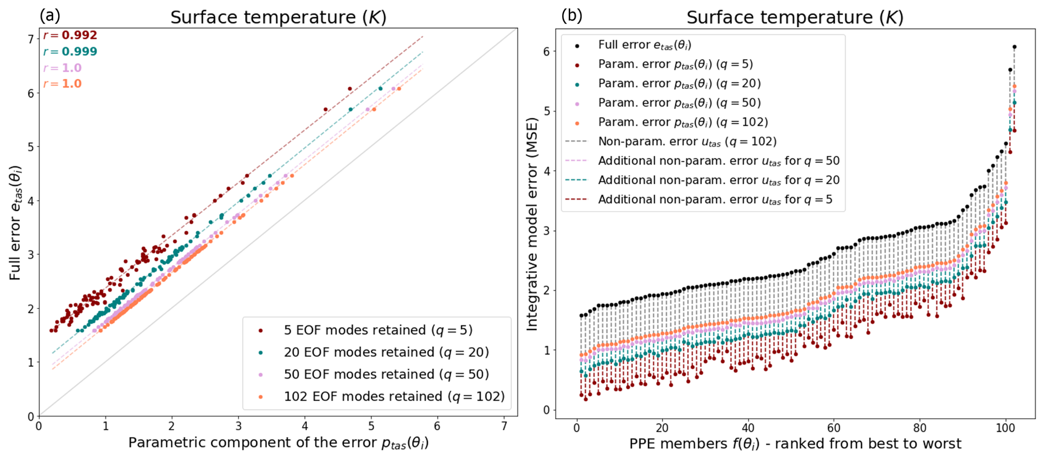
Figure 1 Full model error e_tas and its parametric component p_tas(θ_i) for different truncation lengths, namely q=5 (red dots), q=20 (blue dots), q=50 (pink dots), and q=102 (orange dots). (a) Correlation between the full error e_tas and its parametric component p_tas(θ_i) within the PPEs. (b) Full error partitioning in parametric and non-parametric components in the PPE members f(θ_i) ranked from lowest to highest error.

While retaining a relatively small number of modes (q=5), the correlation between the full model error and its parametric component is already really strong among the PPE members, with a Pearson correlation coefficient of r=0.982 (Fig. 1a). This correlation does not improve a lot when considering higher modes, namely r=0.998 for q=20, and r=0.999 for q=50. This implies that only a relatively small number of modes is required to reproduce the ensemble variance in e_tas(θ_i). The variance in the ensemble spatial error pattern could be described by a small number of degrees of freedom.

However, even for the perfect reconstruction of the model error (when q=102), a non-null, non-parametric component exists, and its ratio corresponds to 26 % of the full model errors averaged over the PPE members, according to Fig. 1. This ratio increases when retaining fewer EOF modes, and a large fraction of the model error pattern is not represented within the parametric component. For example, for a truncation of q=5, the non-parametric component of the error u_tas is 53 % of the total e_tas(θ_i) (on average over the PPEs). Together, this implies that the variance in the model error seen in the PPEs can be explained by a small number of modes, but a significant fraction of this error is not represented within the parametric component of the error decomposition.

3.2 Truncation and parametric emulation

In Sect. 3.1, we demonstrated that the majority of the variance in model MSE can be described as a function of a small number of spatial modes. In an operational model-tuning exercise, we want to make sure that we explain most of the ensemble variance within the truncated EOF basis, so we decided to use a subjective minimum of 85 % of the explained variance when deciding on the truncation length. Now, how does this relate to parametric dependency? We follow Sect. 2.5 to build a linear emulator relating the model parameters θ to the PC coefficients c_tas(θ). Out of a total of 102 simulations, 92 are randomly selected to form the training set. This training set is used to compute the EOF analysis and to derive the least square regression coefficients of the emulator. The out-of-sample emulator performance is then assessed on the remaining 10 simulations, after projection onto the EOF basis. This process is repeated 10 times, with random samples of F used as training sets, to assess the predictive performance of the regression model (i.e., the correlation between out-of-sample predicted c_em,tas(θ) and true c_tas(θ)).

Figure 2a shows both in-sample and out-of-sample skill scores in terms of the mean and standard deviation across the 10 repetitions. The average of out-of-sample performance cumulative on modes is also represented by the red curve (e.g., when q=5, the red curve is the average of the orange curve over modes 1 to 5). We find that the out-of-sample emulation skill declines rapidly when the number of modes increases. This result challenges the utility of including high-order modes in the high-order modes in the spatial emulator of the parametric response (as in Salter et al., 2019), indicating that high-order spatial modes may be too noisy to represent any parametric signal in the ensemble and emulator design considered here. Here we consider an example of truncation at q=18 that will be used in the rest of the study. It corresponds to the point when the average of out-of-sample performance cumulative on modes reaches the arbitrary threshold of 0.5 and explains 94 % of the ensemble variance (respective to our condition of at least 85 % of explained variance).

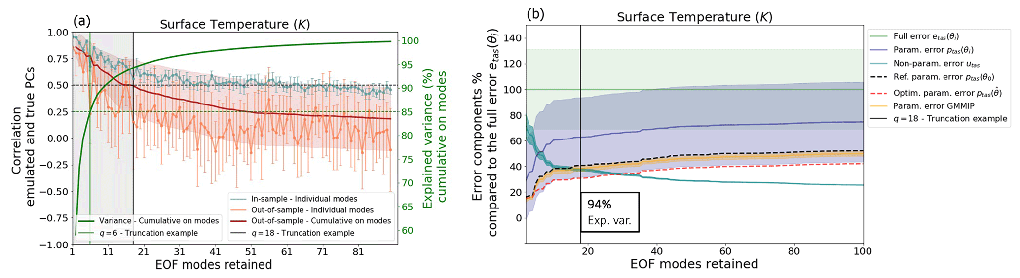
Figure 2 Truncation choice based on parametric emulation and error decomposition. (a) The correlation between the emulated and true principal components (PCs) of the surface temperature EOF for the different modes of variability. The correlation is shown within the training set (blue curve) and the test set (orange curve). The red curve and red shading show the mean correlation averaged over the modes cumulatively. The solid green curve represents the percentage of variance explained when retaining up to q modes of the EOF. The dashed horizontal green line shows a threshold of 85 % of explained variance, and the solid vertical green line is the truncation length needed to satisfy this threshold. (b) The ratio of the error components compared to the full error e_tas(θ_i) (in green) as a function of the number of modes of variability retained. The lines are the ensemble means, and the shadings represent the standard deviations. The plot shows the ratios of the PPE parametric error (dark blue), the PPE non-parametric error (light blue), the reference calibration parametric error p_tas(θ₀) (dotted red curve), and the GMMIP parametric error (orange). An example of truncation at q=18 is represented in both plots by the vertical black line.

Figure 2b shows the ratios between the PPE parametric (dark blue), non-parametric errors (light blue), and the total error (green) as a function of the number of EOF modes retained. We see that for an EOF basis retaining one to five modes, each component represents around 50 % of the total error on average. For the truncation of q=18, the parametric error represents 63 % of the full error on average, and the non-parametric error represents 37 %. This ratio evolves slowly when adding higher modes and, for a perfect reconstruction (q=102), $\frac{p\left({\mathit{\theta }}_i\right)}{e\left({\mathit{\theta }}_i\right)}=\mathrm{74}\mathit{\%}$ and $\frac{u}{e\left({\mathit{\theta }}_i\right)}=\mathrm{26}$ %. But we also note that the large variability in p_tas(θ_i) across the PPE (represented by the standard deviation) is constant, irrespective of the number of EOF modes retained, highlighting the strong dependency of this error component on the parameter values. On the other hand, the variability in the residual error u within the PPE decreases when retaining more EOF modes and is already very small for our truncation example of q=18.

In the context of the Global Monsoons Model Inter-comparison Project (GMMIP; Zhou et al., 2016), an ensemble of 10 atmospheric-only simulations of the CNRM-CM6-1 was run. In this ensemble, the reference model calibration was used, the sea surface temperature (SST) was forced with the same observations as the PPEs, and the members differ by their initial conditions only. This dataset can be used to consider the effect of internal variability on the error decomposition and will be referred to as the GMMIP dataset. The GMMIP dataset can be projected into the PPE-derived EOF basis to compute their associated parametric errors (yellow in Fig. 2b). The variability in the parametric component of the error across the GMMIP dataset is very small and does not depend on the truncation length. The fact that, for q=18 or higher, the variability in u is even smaller than the internal variability in the parametric component confirms that this part of the error is not dependent on the parametric values anymore.

Another point to note from Fig. 2b is that the reference calibration of the model performs well and shows a near-minimal value of the parametric error in the ensemble. Following Eq. (14), we use a multi-linear regression that emulates the parametric component of the model error from the calibration values. This emulator is then used to find an example of near-optimal calibration $\widehat{\mathit{\theta }}$ that minimizes the parametric component of the error. The optimization is done for all the different truncation lengths. As shown in Fig. 2a, the parametric component of the near-optimal calibration is a bit lower than the parametric error of the reference calibration when retaining five or more modes and starts evolving parallel to the PPE mean when retaining seven or more modes. The difference between the PPE mean and this example of optimal calibration becomes constant when q=7 or more, suggesting that there are no improvements in the optimization when adding modes higher than seven.

These results suggest that the EOF basis Γ_q truncated at a relatively small number q=18 is a good representation of the parametric component of the model error pattern. Therefore, the truncation can be used to identify the residual u that does not depend on the perturbed parametric values. Adding further modes has limited impact on the representation of the ensemble variation in the integrated error and does not improve the ability to find near-optimal candidates because of the poor skill of the higher-mode regression prediction. In the following, we will only use a truncation at rank q=18.

3.3 Trade-offs in model candidates

Following the methodology discussed in Sect. 2.6, all emulated members with a parametric error lower than the reference are selected from a 100 000 LHS set of emulations and considered a sub-set of near-optimal calibrations. From this sub-set, 12 candidates have been identified in order to maximize the diversity of model errors. The calibrated set of 12 parameters was then used in the ARPEGE-Climate model to produce actual atmospheric simulations. Of the calibrations, 1 leads to a crash in the model, and 11 others produced the complete atmospheric simulations. The annual mean surface temperature of these 11 candidates was projected onto the EOF basis computed from the 102 members of the PPEs to obtain the principal components. Figure 3 presents the representation of the first five EOF modes by the principal components of the projected model candidates; the closer the candidates are to the observation in the different modes, the lower their parametric error.

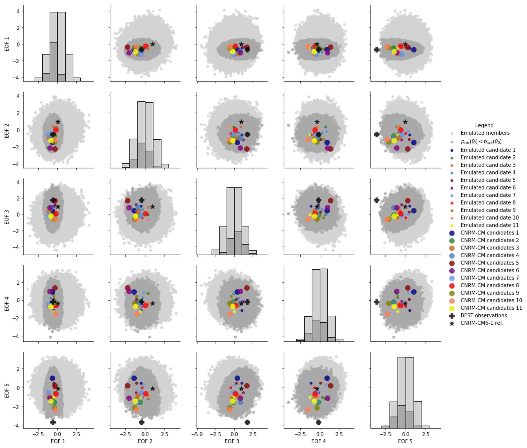
Figure 3 Correlation between the different standardized PC (obtained from the 102-member PPE EOF) for the 100 000 emulated simulations (light gray), the near-optimal emulated members (dark grey; parametric error lower than the reference CNRM-CM6-1 in dark grey), the 11 emulated candidates (colored dots), and the 11 actual CNRM-CM simulations (colored disks). The reference simulation (star) and the observation (cross) are also shown.

Figure 3 provides some confidence in both the emulation skill and the method used for the selection of near-optimal and diverse candidates. Although some differences exist between the emulations of the candidates and their actual atmospheric simulations, all of them show principal components within the near-optimal sub-set of calibrations for the five first EOF modes, thus respecting the condition for near-optimal calibration. Moreover, the candidates seem to explore a range of principal component values as wide as the near-optimal sub-set of calibrations, meaning that we achieve the diversity expected in terms of model errors. In the fifth mode, the projected observations are outside of the emulated ensemble, illustrating that all ensemble members have a non-zero error for this mode, highlighting the existence of a structural bias preventing us from tuning the model to match observations on this axis.

Figure 3 also illustrates the constraints due to the optimization of the principal components on the near-optimal sub-set of calibrations. Indeed, the principal components associated with the first EOF mode of the near-optimal sub-set of calibrations (in dark gray in Fig. 3) span a very reduced range of values compared to the full, emulated ensemble. This result highlights a strong constraint on the first mode of the EOF that is stronger than on the other modes. In other words, the candidates must have a representation of the first EOF mode close to the projected observations in order to achieve a parametric error below the reference. This is an expected result, as we know that the first mode explains most of the PPE variance and that the amount of variance explained by each mode individually decreases in higher modes.

Finally, Fig. 3 illustrates that it is impossible for the model candidates to perform equally well on all modes and fit observations perfectly. Trade-offs exist – even in this space where the variability is driven by the calibration.

Candidate 5, for example, represents modes 1 and 3 very well, with the values of the principal components almost equal to those obtained by projecting the observation on the EOF basis, but is further from the observations in modes 2, 4, and 5. In the same way, candidate 10 performs well for modes 1, 2, and 5 (being the candidate closest to the observation in mode 5, with the observation being outside of the emulated ensemble) but not for modes 3 and 4. Candidate 3 is the best candidate as it is close to the observations for all modes (1 to 4).

All of the 11 candidates have comparable values of their integrated temperature errors (and all are lower than the reference values p(θ₀) and e(θ₀)), and Fig. 3 is a good representation of the trade-offs they have to make in order to minimize this metric. This is a good illustration of the main issue of model tuning; the existence of structural error, which is illustrated here by mode 5, makes a perfect fitting to the observation impossible, and candidates are making trade-offs to achieve the metric minimization. This is well known when considering a classic model-tuning approach in which multiple climatic variables are considered, and the near-optimal calibrations are better at representing certain fields at the expense of others in order to minimize a multi-variate metric. Figure 3 illustrates the problem at the scale of a single field (surface temperature, in this case), highlighting the existence of trade-offs within the near-optimal representation of this field; the temperature will be equally well represented in all the candidates when considering an integrated score (like an MSE), but their spatial error patterns will differ.

3.4 Examples of temperature discrepancy term decomposition

Considering, as described in Sect. 2.4, that the error associated with a near-optimal model is an approximation of the discrepancy term magnitude, the candidates selected here illustrate that near-optimal solutions can be obtained with a diversity of spatial trade-offs that can be made for a minimization problem, even for a single variable output. Moreover, the discrepancy terms can be decomposed in parametric and non-parametric components, as seen in Sect. 2.4. Given the results of Sect. 3.3, there is a good practical case for choosing a low-dimensional basis for calibration – with evidence that it is sufficient to describe the majority of the ensemble error variability and that higher modes are not predictable from parameters. The truncation chosen here is q=18, and Fig. 4 presents the decomposition of the near-optimal candidates errors based on this EOF basis Γ_q=18.

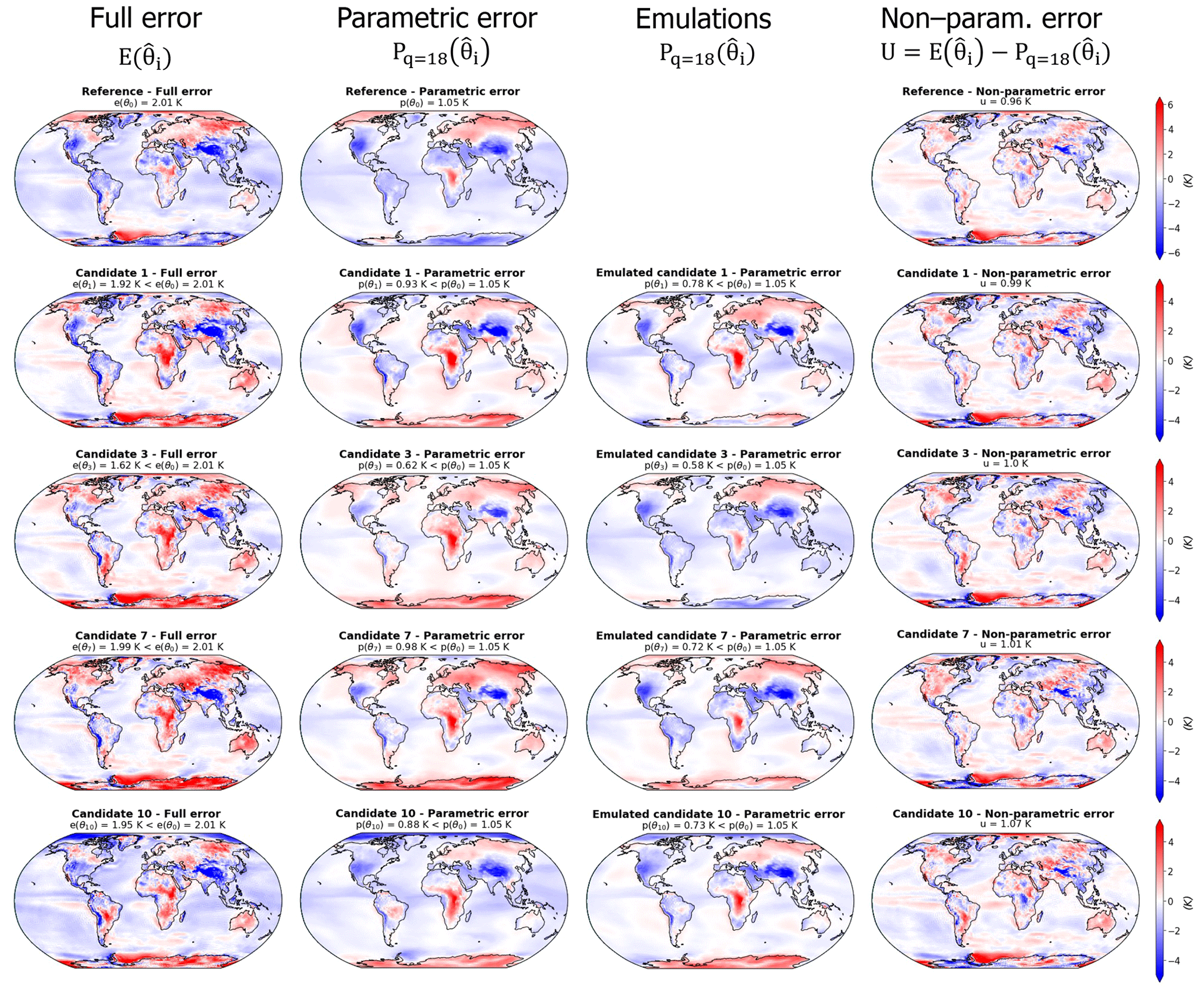
Figure 4 Differences between the simulations of temperature and the observations in BEST (Rohde and Hausfather, 2020) for the four model candidates and the reference. Shown is the decomposition of model errors into parametric and non-parametric components, using the methodology described in Sect. 2, with an EOF basis truncated after mode 18. The left column shows the full differences between simulations and observations, the second column shows the parametric component of this difference, the third column presents the emulation by the linear regression of this parametric component, and the last column is the non-parametric component estimated as the difference between the full error and its parametric component.

For practical reasons, only 4 of the 11 candidates are presented in Fig. 4; the rest of the candidates can be seen in Appendix D (Fig. D1). All of the candidates show full temperature MSEs $e\left({\widehat{\mathit{\theta }}}_i\right)$ between 1.62 and 1.99 K, which is below the MSE of the reference of e(θ₀)=2.01 K. Candidate 7 is the least good, with $e\left({\widehat{\mathit{\theta }}}_{\mathrm{7}}\right)=\mathrm{1.99}$ K and $p\left({\widehat{\mathit{\theta }}}_{\mathrm{7}}\right)=\mathrm{0.98}$ K, and candidate 3 is the best-performing model, with $e\left({\widehat{\mathit{\theta }}}_{\mathrm{3}}\right)=\mathrm{1.62}$ K and $p\left({\widehat{\mathit{\theta }}}_{\mathrm{3}}\right)=\mathrm{0.62}$ K. The quality of the statistical emulations of the parametric component varies, depending on the candidate, and the biases over Antarctica are poorly captured by the emulations. We note that the emulation of candidate 3 shows a rather different parametric error than the actual pattern, with an opposite sign of the biases over Antarctica, Australia, India, and Argentina, as well as a strong underestimate of the positive bias over central Africa. For candidate 10, the statistical emulation of the parametric error's spatial pattern is really close to the truth. We discuss the uneven performance of the statistical predictions in Appendix C and argue that the emulator skill is mostly limited by the size of the training set.

As stated before, near-optimal candidate errors are our best estimate of the discrepancy term diversity. The full errors shown in Fig. 4 display features common to the four candidates and the reference, namely negative biases over the mountain regions (Himalaya, Andes, and North American mountains) and a positive bias over central Africa. However, the magnitude and position of these biases vary from one model to another, with a particularly strong negative bias over North America in candidate 1 and a strong positive bias over central Africa in candidate 3, for example. This diversity is highlighted when looking at the parametric components of the candidate errors, showing a variety of error signs and patterns over the poles (especially Antarctica), the south of Europe, India, North Africa, and Canada.

The non-parametric components of the errors are smaller and qualitatively similar among the candidates, confirming that they are not strongly controlled by the parameter values. In other words (as expected by the method), the first few modes of the EOF analysis are enough to represent the diversity of the model error spatial trade-offs among a sub-set of near-optimal candidates. Moreover, the method allows us to visualize and compare these trade-offs through the spatial representation of the parametric component (Fig. 4).

4 Second application: multi-variate error

4.1 Variables, EOF analysis, and truncations

The univariate analysis conducted in Sect. 3 illustrates qualitatively the potential for trade-offs and multiple near-optimal solutions of the climate model optimization problem. In this section, we considered a single univariate metric, allowing us to select 12 near-optimal candidates maximizing the diversity of spatial error patterns and trade-offs among the different EOF modes.

Rohde and Hausfather (2020)Huffman et al. (2009)Saha et al. (2010)Loeb et al. (2018)Loeb et al. (2018)

Table 1 Table of observable variables used in this study, plus citations for the data products used. Note that TOA stands for top of atmosphere.

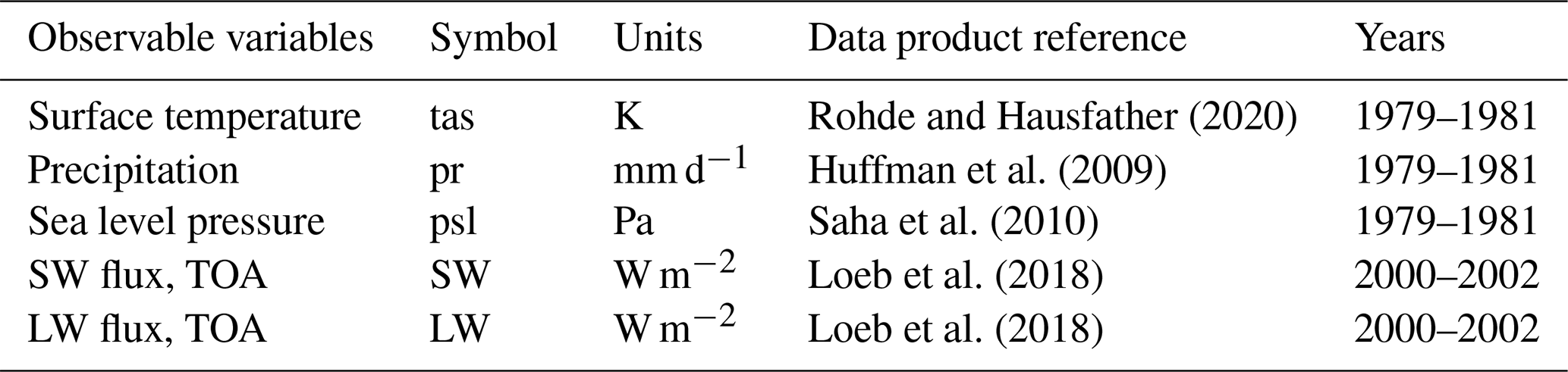
In an operational GCM-tuning application, the metric considered must encompass multiple climate fields, and the optimization results in trade-offs between different univariate metrics, with near-optimal models better representing some fields at the expense of others. The general solution to the model calibration for operational use requires the consideration of a wide range of climatological fields spanning model components, including mean state climatologies, assessment of climate variability, and historical climate change. This is inherently more qualitative – requiring subjective decisions on variable choices and weighting, which are beyond the scope of this study. However, we can consider an illustration of a multi-variate application, based on five climatic fields: the surface temperature (tas), the precipitation (pr), the shortwave (SW) and longwave fluxes (LW) at the top of the atmosphere, and the surface pressure (psl). The model errors will be defined as the MSE between the model simulations and the observational dataset lists in Table 1. As for the univariate application, EOF analysis of the PPE variance is computed for the annual means of the different climatic fields, and the EOF truncation choices depends on the parametric emulation skill and the error decomposition.

Figure 5 presents the performances of multi-linear regressions in the prediction of the principal components for the five fields, and we note a strong decrease in the out-of-sample prediction skills as we move toward higher EOF modes for all climatic fields. Based on this result, it is clear that, as for the univariate application, the optimization should only retain the first few modes. The truncation lengths should be different from one climatic field to another as the linear regressions perform the best for the SW fluxes but have a rather poor out-of-sample skill in terms of sea level pressure, for example. Examples of EOF truncations are given in Fig. 5, based on an arbitrary threshold of 0.5 for the averaged correlation coefficient of predicted and true out-of-sample principal components. We also ensured that the truncated basis explained at least 85 % of the ensemble variance. These examples suggest that it is possible to retain up to 28 EOF modes for the top-of-atmosphere (TOA) SW flux univariate metric, whereas no mode higher than 8 should be considered for the sea level pressure in order to keep satisfying statistical predictions. Moreover, some variables require more EOF modes than others in order to explain most of the ensemble variance. For precipitation, we need to keep 18 EOF modes in order to explain 85 % of variance, whereas for sea level pressure, the first 8 EOF modes explain 92 % of the variance. However, for every climatic field considered, the variance in the model errors within the PPE is already very-well represented by the first five EOF modes, as suggested by the correlations between reconstructed and full errors (Fig. 6). Considering these truncation lengths, the PPE mean parametric component represents 80 % of the full PPE mean error for the TOA SW fluxes but only 66 % for the sea level pressure.

The error reconstructions presented in Fig. 6 are the sums of the parametric components of the errors p_j(θ_i) and the PPE mean non-parametric components u_j,mean. As expected, the PPE mean non-parametric components decrease as higher EOF modes are retained for the reconstruction but are never equal to zero (even for a full reconstruction of q=102). This is due to the fact that observations can never be fully captured by their projections into the model EOF basis (Fig. 6). As presented before, the parametric component p_j(θ_i) can be emulated with multi-linear regressions, and the PPE mean non-parametric component u_j,mean can be used as an approximation to reconstruct the full error e_j(θ_i). This method succeeds in producing high correlations between the reconstructions and the actual full model errors among the PPE, with an offset due to the non-parametric component variability across the PPE, which decreases when retaining more EOF modes. Even though higher EOF modes are not well predicted by the emulators (Fig. 5), they also explain small fractions of the model error variances. As a result, the performances of the emulators when predicting model errors are much more sensitive to the climatic field considered than to the number of EOF modes retained.

On the other hand, the reference calibration CNRM-CM6-1 remains one of the best models of the PPE for most of the climatic fields and can be considered near-optimal in the ensemble. Therefore, its model bias can be seen as a representative of the CNRM-CM discrepancy term. Indeed, the reference CNRM-CM6-1 is the best model for surface pressure and one of the best for precipitation and TOA fluxes, but several PPE members outperform it for surface temperature. This is a simple illustration of a complex tuning problem and based on the results we obtained in the univariate application. It seems likely that comparably performing parameter configurations potentially exist for a multi-variate tuning problem, making different model trade-offs among both climatic fields and EOF modes representative of univariate errors (Fig. 3). In the next section, we will attempt to identify some of them in order to illustrate the different choices that could be made when tuning a climate model.

Figure 5 Truncation choice based on parametric emulation and error decomposition for five climatic fields: surface temperature, precipitation, TOA SW fluxes, TOA LW fluxes, and surface pressure. The same legend is used as in Fig. 2, and the observations used are listed in Table 1.

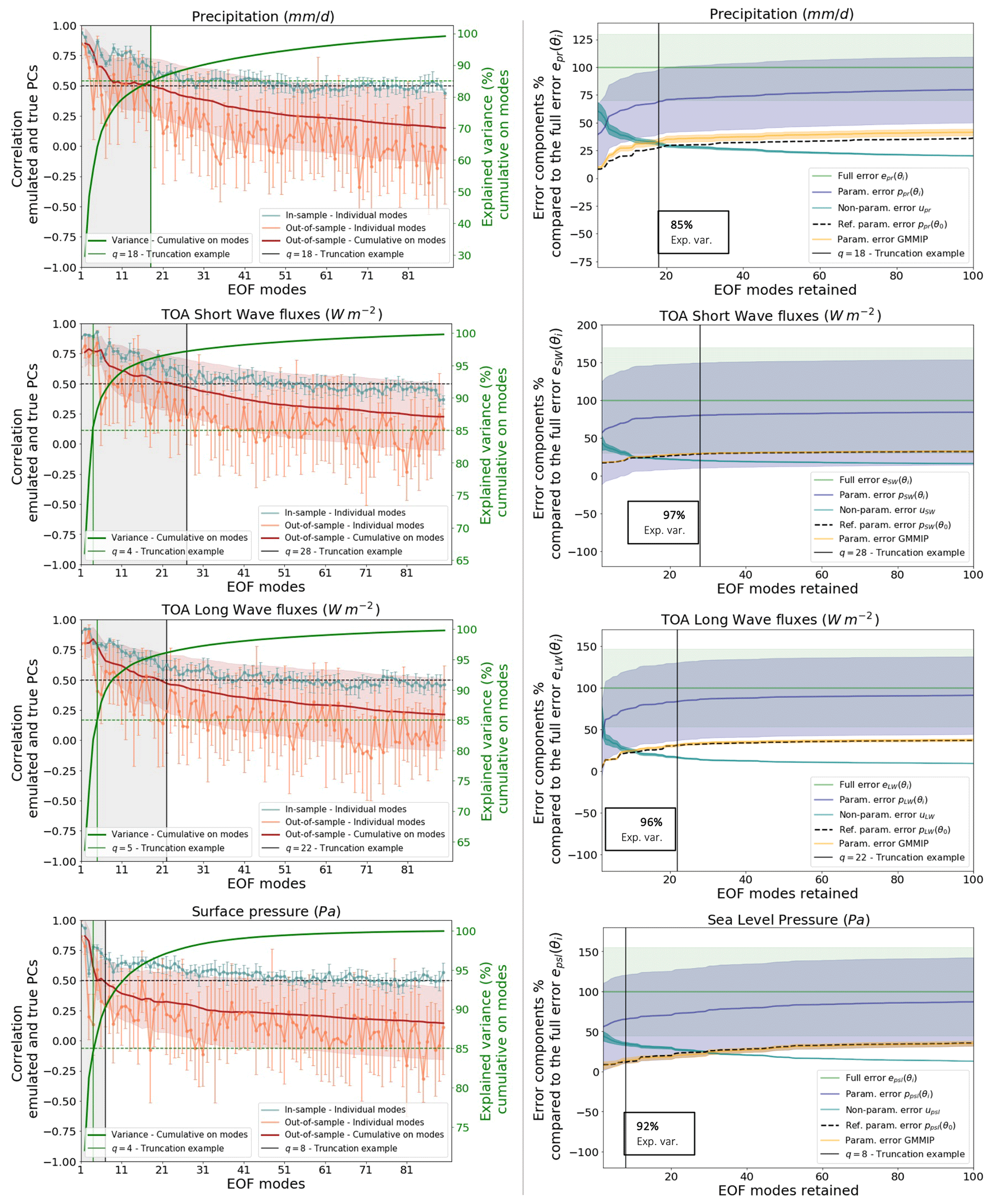
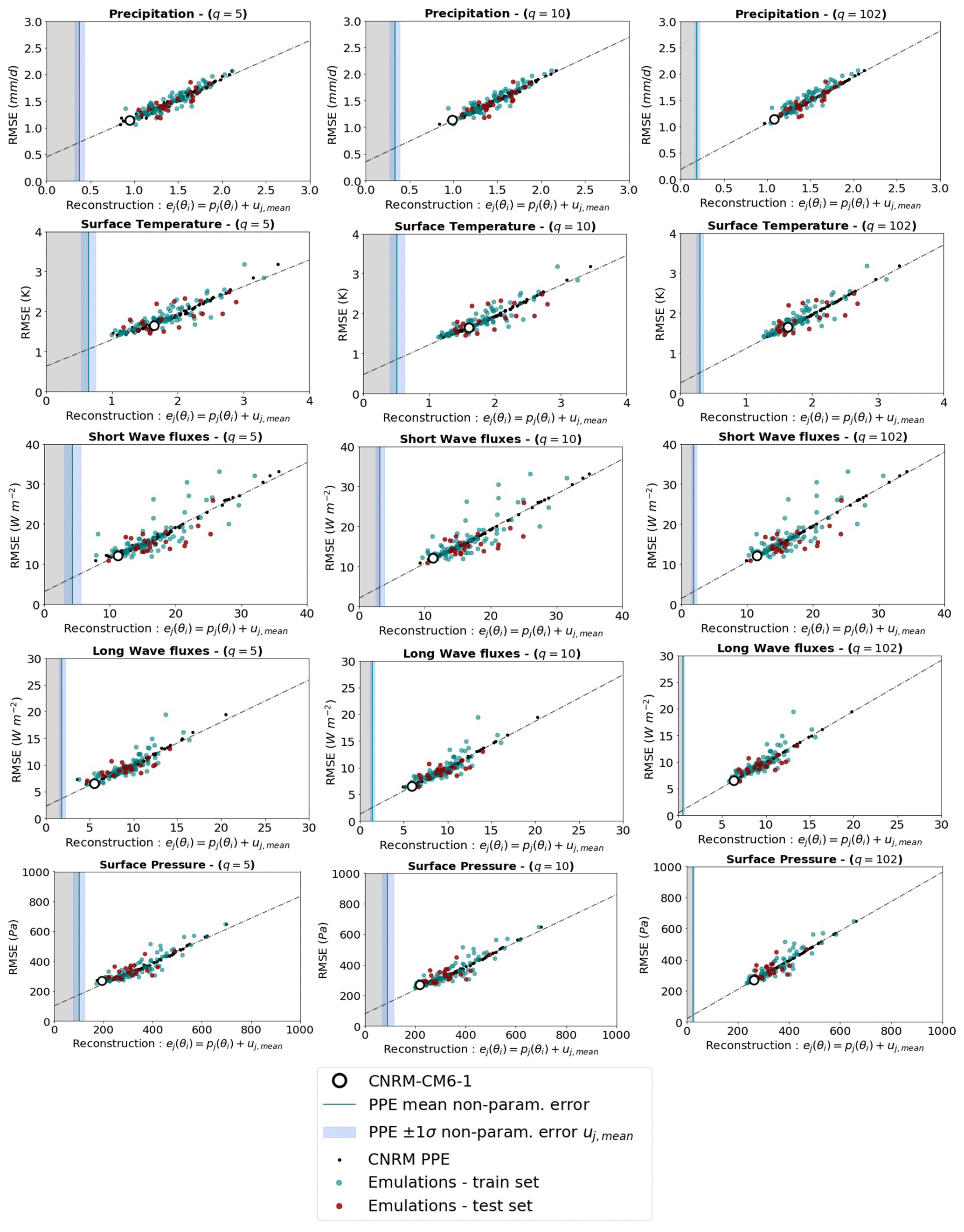
Figure 6 Correlations between full errors (coordinate) and EOF-based reconstructions of these errors (abscissa), using different truncation examples, when retaining 5 (left column), 10 (center column), and 102 EOF modes (right column). Results are presented for the CNRM PPE (black dots) and for statistical predictions of the PPE using linear regressions trained on 80 % of the data (green dots) and tested on the other 20 % (orange dots). For each PPE member or emulation, the error reconstruction is the sum of the parametric component of the errors p_j(θ_i) and the PPE mean non-parametric component u_j,mean (blue line). The variability in u_j among the PPE is represented by the standard deviation σ and the range ±1σ (light blue shading).

4.2 Candidate selection in a multi-variate context

The results in terms of integrated multi-variate skill scores e_tot(θ_i) are presented in Fig. 7. Among the 12 selected candidates, 2 lead to an incomplete simulation and will not be presented here. None of the 10 remaining candidates (light blue dots) shows a multi-variate skill score lower than the CNRM-CM6-1 reference model (dashed orange line). However, all of them have a lower error than the PPE mean (red disk) and three of them are in the low tail of the PPE distribution (below the dashed red line). Moreover, most of the CMIP6 models have undergone a tuning process and are considered to represent the control climate satisfactorily. We can therefore use the CMIP6 ensemble as an indicator of the tolerance that can be given to this multi-variate error. Here we considered the outputs of 40 CMIP6 models that have been interpolated onto the CNRM-CM grid before computing the error. It appears that 9 CNRM-CM candidates selected here have a lower error than the mean of the 40 CMIP6 models (green disk). These nine CNRM-CM candidates are part of the interval of plus or minus 1 standard deviation of the CMIP6 error centered around the error in the CNRM-CM6-1 reference model (orange area), indicating that they can be considered “as good as” the CNRM-CM6-1 reference model given the tolerance considered here. The 10th candidate is above this interval but is still very close to the CMIP6 ensemble mean and better performing than several CMIP6 models.

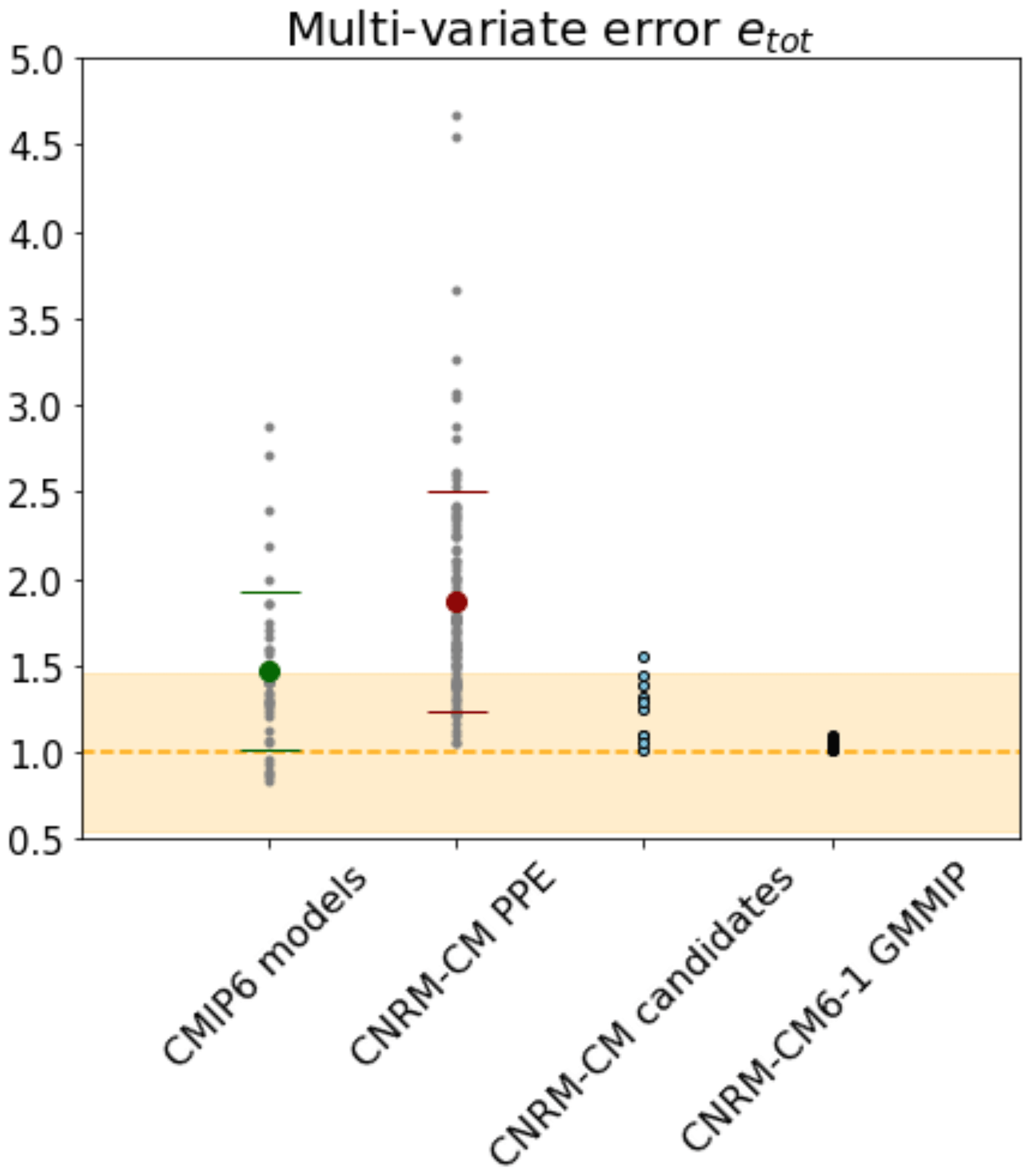
Figure 7 Multi-variate error e_tot for the CMIP6 models, the CNRM-CM PPE members, the selection of 10 CNRM-CM candidates and the GMMIP dataset. Each small dot corresponds to a model, the bigger dots correspond to the ensemble means, and the dashes are the standard deviations. The dashed orange line at 1.0 represents the CNRM-CM6-1 reference model error. The orange area indicates the interval of plus or minus 1 standard deviation of the CMIP6 errors centered around the CNRM-CM6-1 reference model error.

Figure 7 is also presenting the multi-variate error among the 10 simulations from the GMMIP dataset. The 10 perturbed parameter candidates are much more diverse in terms of integrated model error that the 10 perturbed initial conditions members. When considering a multi-variate score, it is clear that the effect of internal variability is very small compared to the effect of varying the model parameters.

4.3 Diversity of error patterns among candidates

As described in Fig. 7, the 10 CNRM-CM candidates present a satisfactory multi-variate error compared to the CMIP6 ensemble, with 9 of them performing comparably to the CNRM-CM6-1 reference model, while showing a significant diversity compared to the CNRM-CM GMMIP ensemble. We are now interested to see how this diversity translates in terms of the spatial patterns of the univariate errors and trade-offs among the variables.

Here again, for practical reasons, a sub-set of four candidates is presented in Fig. 8, and the rest of the candidates can be seen in Appendix E. Within the four candidates presented in Fig. 8, we have selected the best-performing model (candidate 5) and the worst-performing model (candidate 1). All the candidates have features common to the CNRM reference model (Roehrig et al., 2020), namely an overestimate of the tropical precipitation and large SW fluxes biases over the mid-latitude eastern border of the Atlantic and Pacific oceans. However, they all have a better representation of surface temperature than the reference model. None of the candidates shows a better representation of precipitation, sea level pressure, or LW outgoing fluxes than the reference, and candidates 1, 2, 5, and 9 provide a better representation of the SW outgoing fluxes.

Moreover, some differences exist between the spatial patterns of the candidate errors. Candidate 10 is the model configuration with the lowest MSE of precipitation ($e_{\mathrm{pr}}\left({\widehat{\mathit{\theta }}}_{\mathrm{10}}\right)=\mathrm{2.18}$ mm d⁻¹; still higher than the reference) but is also showing important tropical biases in the radiative fluxes (positive in SW and negative in LW) in the same regions where the model overestimates the tropical precipitation, suggesting a biased representation of tropical clouds. Candidate 5, on the other hand, has a better representation of the radiative fluxes in these regions, with a better representation of SW fluxes than the reference and the best representation of LW among the candidates, suggesting a better representation of tropical clouds. However, candidate 5 is presenting the same biases in precipitation as candidate 10 but with an even higher MSE.

Candidate 1 in the worst-performing model of the whole selection, with a total MSE of $e_{\mathrm{tot}}\left({\widehat{\mathit{\theta }}}_{\mathrm{1}}\right)=\mathrm{1.56}$. This is mostly due to important biases in precipitation, sea level pressure, and LW flux representations. Candidate 1 presents strong positive tropical biases in LW fluxes over the northern part of South America, central Africa, and Indonesia. These areas corresponds to dry biases in the map of precipitation. Over the tropical oceans, it is one of the candidates that is not showing the negative LW and positive SW tropical biases; other examples can be found in candidates 3, 8, and 9 (Fig. E1). These candidates all have positive LW biases over the tropical continents and fewer biases over the tropical oceans. Interestingly, this is one of the candidates with the best representation of SW fluxes with candidate 9 (Fig. E1), which has a lower MSE. The SW flux biases over the mid-latitude eastern border of the Atlantic and Pacific oceans seem to be reduced in these two candidates compared to the other models and the reference.

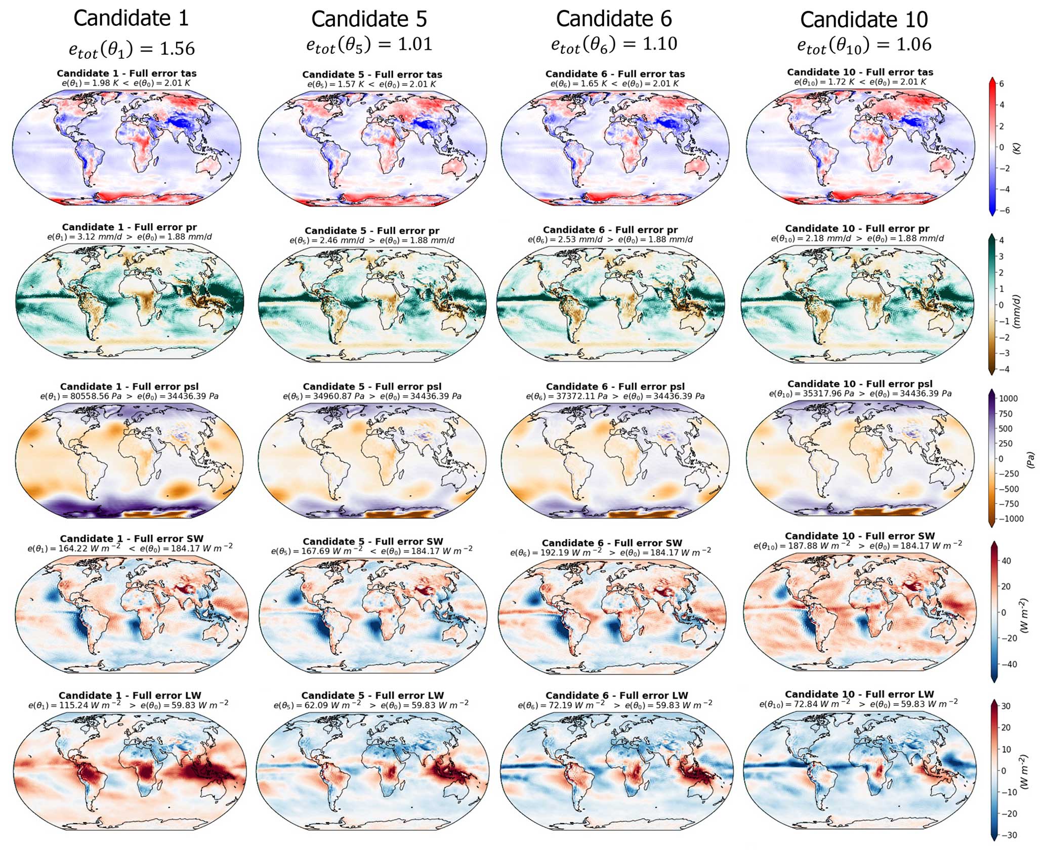
Figure 8 Differences between the simulations and the observations (Table 1) for the four model candidates and the five variables considered (surface temperature, precipitation, sea level pressure, short- and longwaves, and top-of-atmosphere fluxes). Each column represents a model candidate, and each row corresponds to a variable. The green dots highlight the cases for which the RMSE is lower than the CNRM reference model.

Candidate 5 is the best-performing candidate in terms of multi-variate score and shows errors lower than the CNRM reference model for surface temperature and SW fluxes (Fig. 8). Candidate 5 shows a LW error map similar to candidates 6 and 10 but with a reduction in the bias amplitudes. We can assume that the model is better representing tropical clouds, but this does not translate to the best representation of tropical precipitation within the selection.

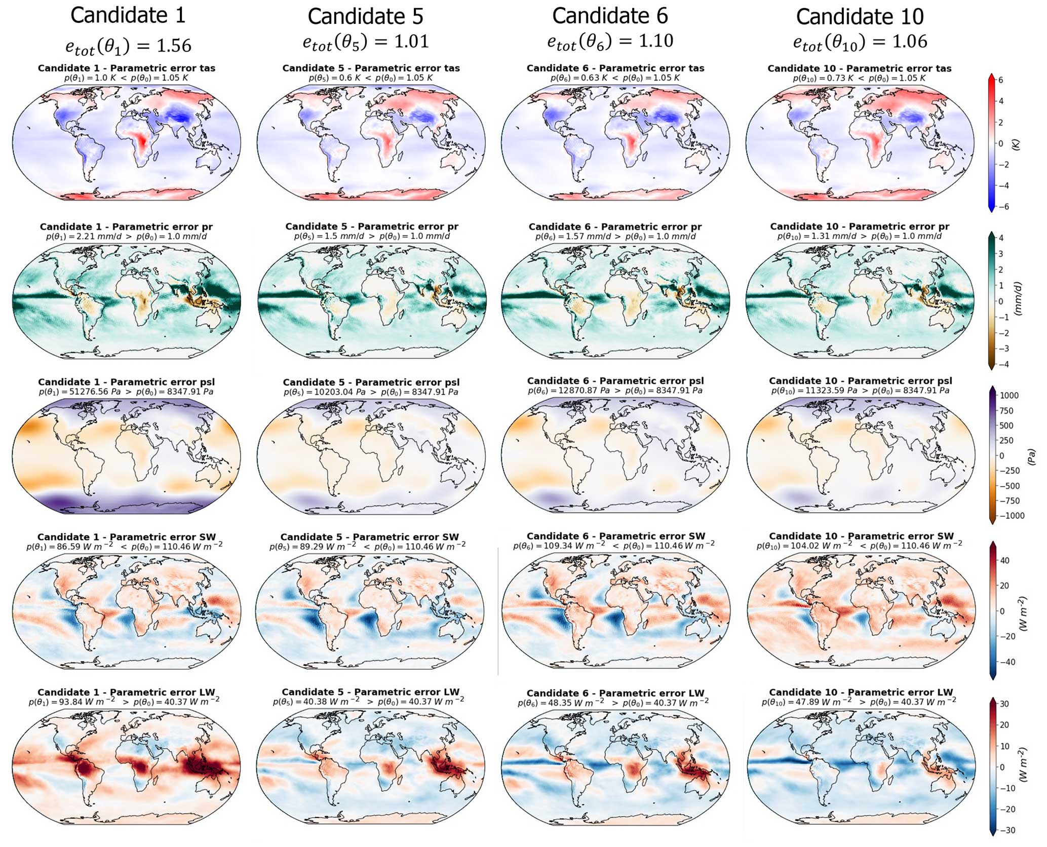
Figure 9 Parametric component of the differences between the simulations and the observations (Table 1) for the four model candidates and the five variables considered. Each column represents a model candidate, and each row corresponds to a variable. The decomposition of model errors in parametric and non-parametric components is based on the methodology described in Sect. 2.4, with the EOF bases truncated following the examples given in Fig. 5: 18 modes for tas and pr, 8 modes for psl, 28 modes for SW, and 22 modes for LW.

Figure 10 Non-parametric component of the differences between the simulations and the observations (Table 1) for the four model candidates and the five variables considered. These components are the differences between Figs. 8 and 9.

4.4 Examples of discrepancy term decomposition

Following the method described in Sect. 2.4, the full error patterns presented in Fig. 8 can be decomposed into a parametric components (Fig. 9) and non-parametric components (Fig. 10). The EOF truncation lengths used for this decomposition are based on the examples given in Fig. 5, with 18 modes for tas and pr, 8 modes for psl, 28 for SW, and 22 for LW.

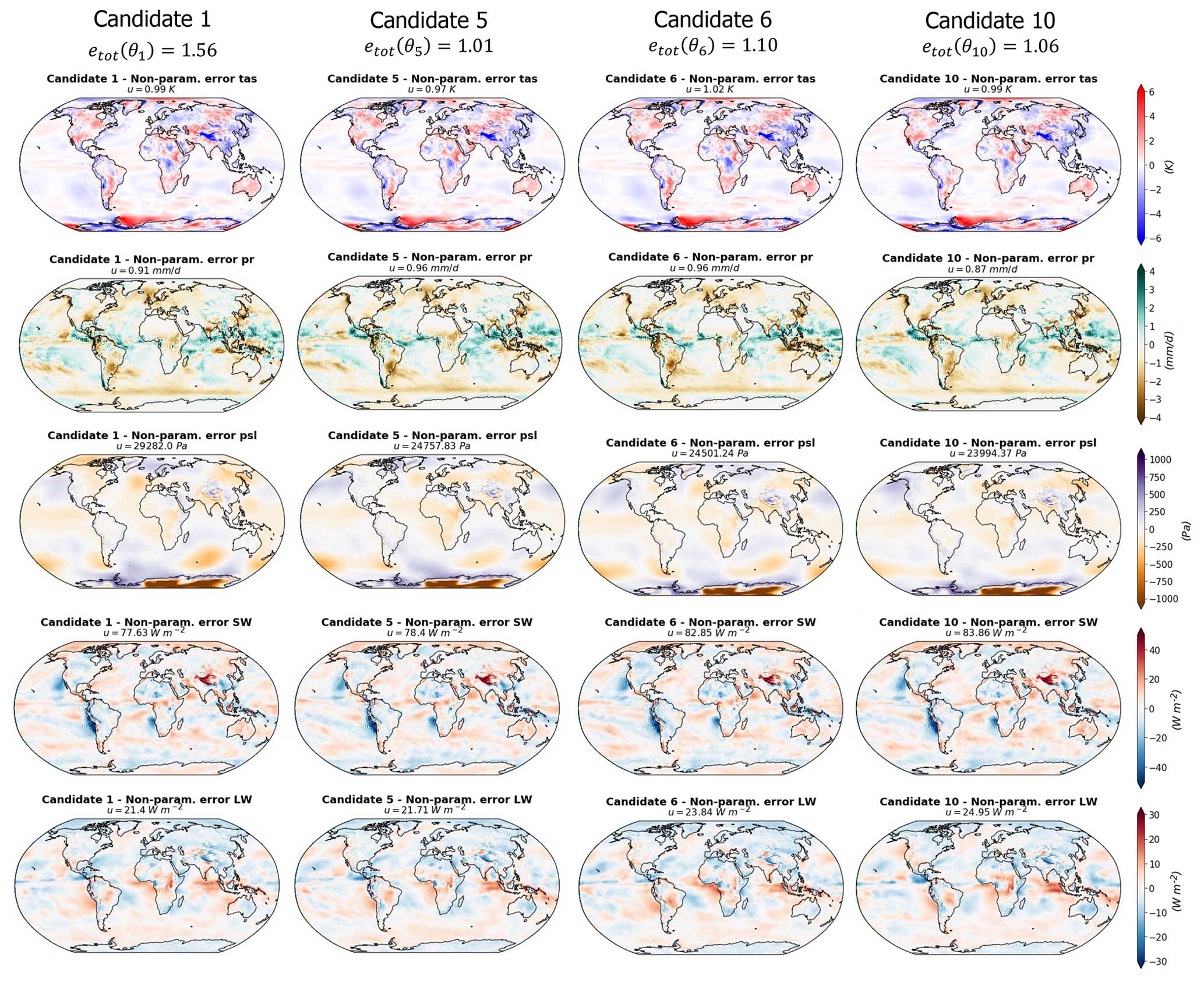
As expected, the candidates' parametric component error patterns resemble the full error patterns – with as much diversity in between the candidates (Fig. 9). The non-parametric components, on the other hand, are more patchy, are smaller in terms of amplitude, and are common to all the candidates (Fig. 10). This validates the method; we were able to select a set of candidates with diverse error patterns and to isolate the error component that is unaffected by parameter variation from the component that varies during model tuning.

A notable feature of these candidate error decompositions is the SW error patterns. The non-parametric component of the SW error appears very patchy but contains a small part of the negative biases over the oceanic mid-latitude eastern border that we described in the full error patterns that are directly at the continental border (Fig. 10). The main part of these biases is presented in the parametric component of the error (Fig. 9). This result suggests that such biases could be enhanced or reduced by varying the model parameters, but part of them is non-parametric and directly linked to the physics of the model.

In conclusion, when considering error patterns and multi-variate illustrations, the effective degrees of freedom in the model performance optimization might be smaller than expected. Our method allowed for an empirical exploration of the key trade-offs that could be made during the tuning, providing interesting information about model non-parametric biases and examples of alternative model configurations.

5 Conclusions

This study presented a new framework, based on a PPE of a CMIP6 general circulation model, allowing for the empirical selection of diverse near-optimal candidate calibrations. Using the best input assumption (Rougier, 2007), we assume that these candidates sample the distribution of atmospheric model discrepancy term. These discrepancy term can be decomposed into parametric and non-parametric components using a PPE-derived EOF basis. The candidates are selected from a PPE of the CNRM-CM atmospheric model. The optimization is based on multi-linear predictions of the parametric components of the model errors from a 100 000 LHS of the perturbed parameters. The candidates are considered near-optimal when their emulated parametric components are lower than the reference parametric component and are selected to exhibit pattern errors as diverse as possible within this near-optimal sub-space using a k-median clustering algorithm. As such, the sub-set of candidates offers a diversity of model errors that sample the CNRM-CM model discrepancy term distribution while exploring different trade-offs.

The decomposition of the discrepancy terms depends on the truncation choice; the non-parametric component increases when retaining more EOF modes, which comes at the expense of the parametric component. However, we argue that there are no particular benefits from retaining high-order EOF modes for two reasons. First, the performance of the predictions quickly decreases for the high-ranking EOF modes, which suggests that these modes are not very predictable from the parameter values. Then, there is the fact that the first few modes are sufficient to reconstruct the PPE variance of the model errors for the five climatic fields considered here and that high modes explain a very small fraction of the PPE variance. Therefore, retaining more EOF modes will increase the part of the model error represented by the EOF basis, which is called the parametric component, but will not improve the optimization.

In the first step, the method was validated for surface temperature error, revealing a diversity of trade-offs among different EOF modes when considering diverse but near-optimal candidates. These trade-offs indicate the presence of a parametric component in the discrepancy terms, which no candidates could eliminate completely. The non-parametric component, on the other hand, is independent of parameter choice and very similar from one candidate to another. These model candidate errors are considered to represent empirical examples of the model discrepancy term for temperature and can offer insights for model developers. In the second step, the framework was applied in a multi-variate context. Trade-offs were observed in error patterns across climatic fields, with different candidates excelling in various aspects. All of the candidates were selected with an emulated parametric error lower than the reference but showed, in practice, higher parametric errors. This result can be attributed to the limitations of the emulators. However, as discussed in Appendix C, our capacity to train emulators is fundamentally limited by the sample size available, which is rather small in this study (102 simulations). The use of a non-linear emulator, such as a Gaussian process, often used in automatic tuning applications (Williamson et al., 2013; Hourdin et al., 2023), could help improve predictions, provided we can increase the size of the PPE. In summary, nine candidates achieved integrated multi-variate scores within CMIP6 ensemble standards, but none of them performed better than the reference model.

We have demonstrated that this approach is practically useful for the following different reasons:

1. The effective degrees of freedom in the model performance's response to parameter input are in fact relatively small, allowing a convenient exploration of key trade-offs.

2. Higher modes of variability should not be included because they cannot be reliably emulated, and they do not contribute significantly to the component of model error controlled by model parameters.

3. As such, the reference model version shows that the lowest integrated performance metric and historical common practices for parameter tuning could be more robust than often assumed.

4. However, there remains the potential for comparably performing parameter configurations by making different model trade-offs.

Though we do not attempt it here, the discrepancy estimate could be used in parallel with a history-matching approach, such as Salter et al. (2019), or a Bayesian calibration (Annan et al., 2005) to yield a formal probabilistic result. Enhancing the PPE size would allow for better statistical predictions, maybe through the use of Gaussian processes as statistical models. We could also consider seasonal metrics instead of the annual average, as suggested in Howland et al. (2022). Another important caveat of this study is that we did not consider the observational uncertainty. Indeed, additional analyses suggest that our results are sensitive to the observational dataset used. Therefore, defining a formal way to include the observational uncertainty in our method for candidate selection would be a valuable improvement of the method. Finally, performing sensitivity analysis could help us better understand the effect of each parameter on the biases we observed, potentially leading to a selection of a meaningful sub-set of parameters for a new wave of simulation in an iterative process.

In summary, we argue that the model discrepancy term can be represented as a sum of two parts – a component which is insensitive to model parameter changes and a component which represents parameter trade-offs, which manifest as an inability to simultaneously reduce different components of the model bias (e.g., in joint optimization of different regions or fields). We further argue that a parameter calibration done by hand could be more tractable than often assumed, and the reference versions may often be the best model configuration achievable in terms of integrated multi-variate metrics. This is a feature we see evidenced here by the high performance of the reference simulation (but also reported in similar past PPE efforts) (Sanderson et al., 2008; Li et al., 2019). Finally, we demonstrate a practical method for utilizing these concepts for the identification of a set of comparably performing candidate models that can inform developers about the diversity of possible trade-offs. The selection of diverse candidates can help better understand the limits of model tuning to reduce model error, identify non-parametric biases that are not visible when looking at the full model error, and help choose the model configuration best suited to the research interest. Moreover, the diversity of model errors can reflect a diversity of future climate responses (Peatier et al., 2022; Hourdin et al., 2023), and selecting diverse candidates will help the quantification of uncertainty in climate change impact studies.

Appendix A: Perturbed parameter

Table A1 Description of the 30 perturbed parameters.

Appendix B: Clustering analysis and sensitivity to the number of clusters

For both applications, the k-median analysis is repeated 10 times for different values of k, and the average of inertia and Dunn indexes is presented in Fig. B1. The inertia sensitivity test suggests that we could chose a value of k between 10 and 20 to be in the elbow of the curve for both applications. Then, even though it is less obvious for the multi-variate application, the results suggest that we should not take a value of k that is too high, as the Dunn index tends to decrease. Based on these two criteria, we have decides to keep 12 clusters for the analysis, i.e., k=12.

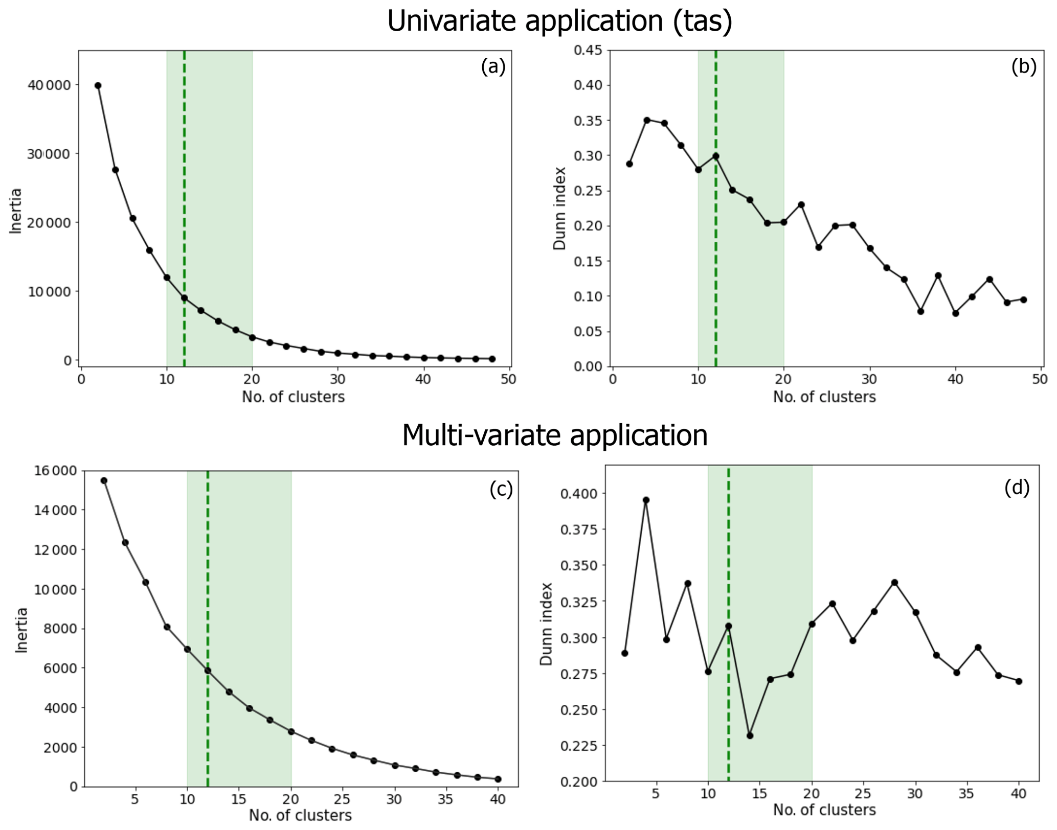
Figure B1 Sensitivity test of the clustering analyses for the univariate (first row) and multi-variate (second row) applications. The inertia criteria (a, b) and the Dunn indexes (b, d) are shown, depending on the number of clusters (x axes). The shaded green areas present the acceptable number of clusters, following the elbow method applied to the inertia. The dashed green line shows the number of clusters retained for our analyses, i.e., k=12 in both applications.

Appendix C: Evaluation of the statistical predictions

The emulators used in this study are multi-linear regressions (MLRs) taking the model parameters as input and predicting the principal components (PCs) used to reconstruct the 3D variables and the parametric model errors when comparing with observations. The ensemble size of the PPE is very limited (102 simulations), and our capacity to train emulators is fundamentally limited by the sample size available. However, in 10 random selections of out-of-sample test sets, we obtain an average correlation of 0.7 between the predictions and the true values of total error (Fig. C1c), with a RMSE between predictions and true values representing 8 % of the total parametric error (Fig. C1f), which is sufficient to validate the use of this model for our study.

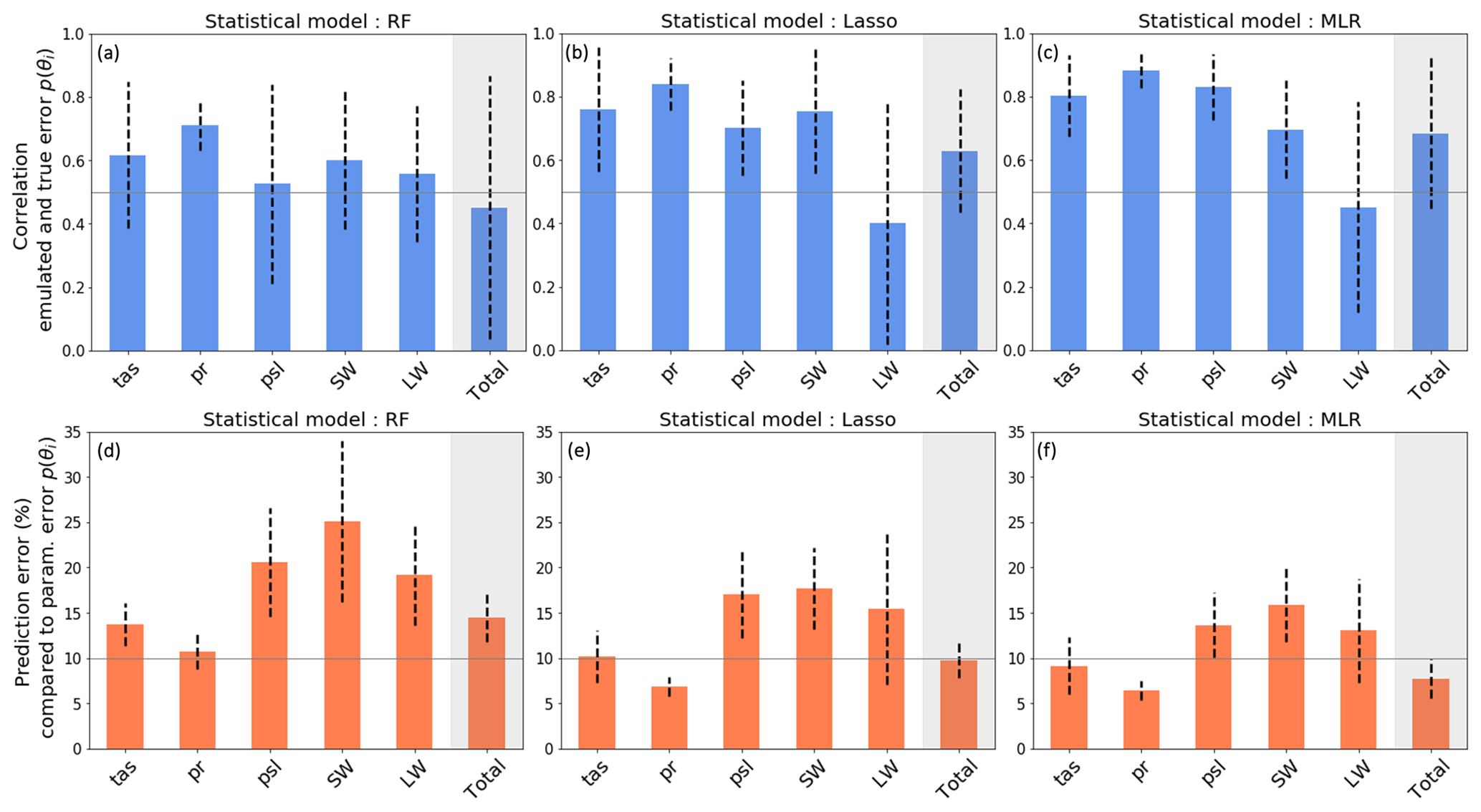
Figure C1 Correlations and RMSE (in %; compared to the true values) between emulated and true parametric components of the errors within a test set representing 10 % of the dataset. The evaluation is repeated 10 times with random sampling of training and test sets, and the mean and standard deviation among these 10 evaluations are represented by the bars and the dashed lines, respectively. Performances are shown for (a, d) a random forest, (b, e) a lasso regression, and (c, f) the multi-linear regression used in this analysis. The EOF truncation lengths used to compute the parametric error are presented in Figs. 2 and 5.

However, results suggest that there is room for improvement, especially in the prediction of the LW errors, and that another model could improve the predictions, as is the case with the random forest model. The error bars associated with the prediction of the total error suggest that the MLR performance is sensitive to the test set selected and that the model will perform unevenly across the parameter space. Thanks to variable selection and regularization, the lasso model seems a bit less sensitive to the test set selection for the prediction of total error, but the prediction of LW error is still a limitation. It seems that using a non-linear emulator could improve certain aspects of the predictions, though enhancing the size of the ensemble would be a necessary prerequisite to try to improve our statistical predictions.

Appendix D: First application: additional candidates

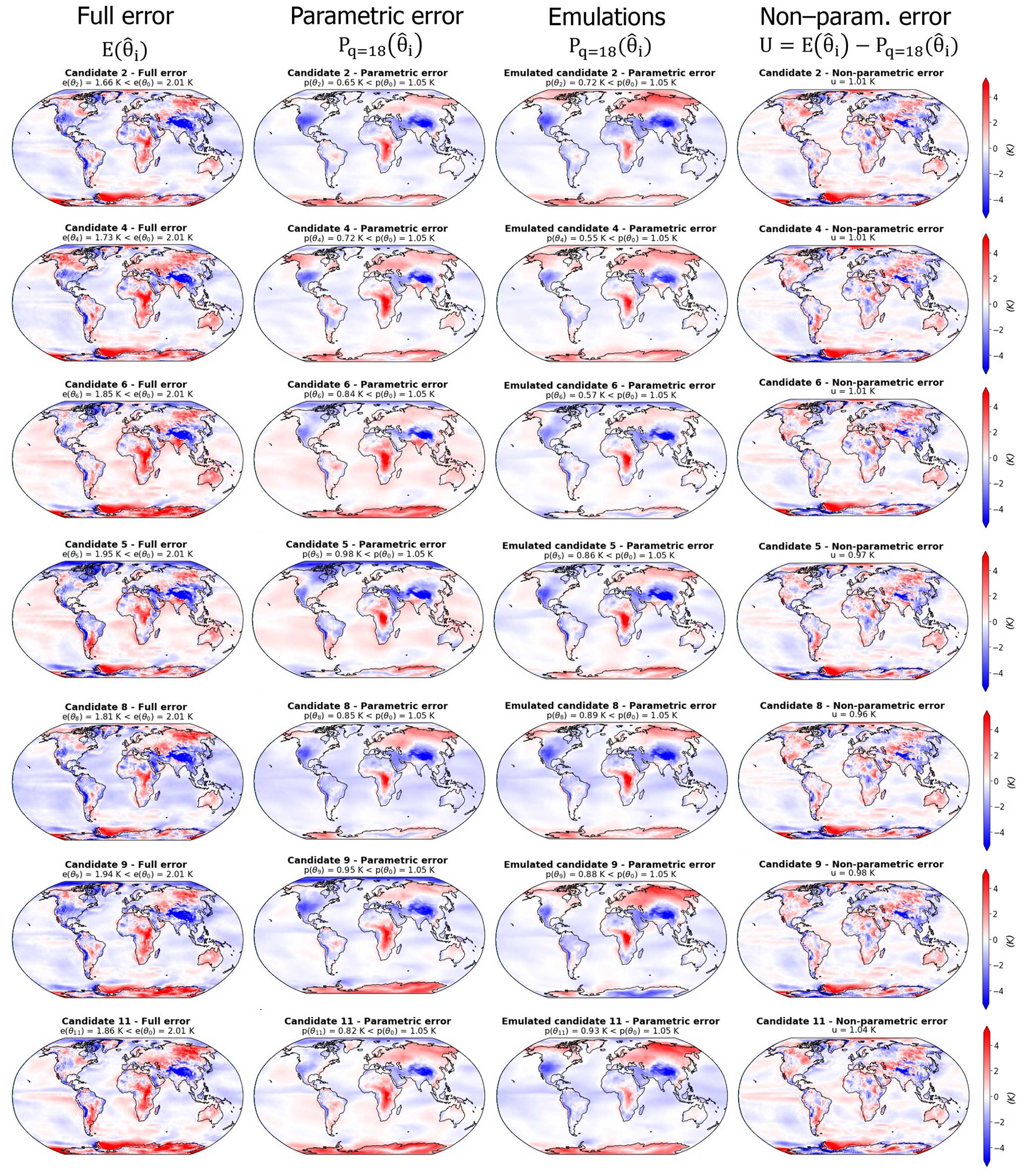
Figure D1 Decomposition of surface temperature error in the first sub-set of candidates. Same as Fig. 4 for additional candidates.

Appendix E: Second application: additional candidates

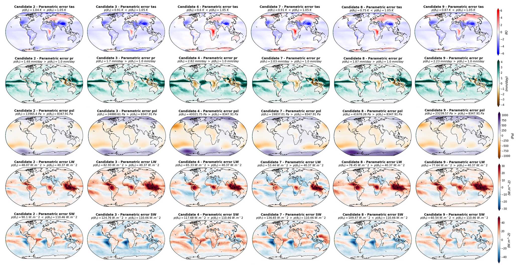
Figure E1 Full model errors in the second sub-set of candidates. Same as Fig. 8 for additional candidates.

Figure E2 Parametric model errors in the second sub-set of candidates. Same as Fig. 9 for additional candidates.

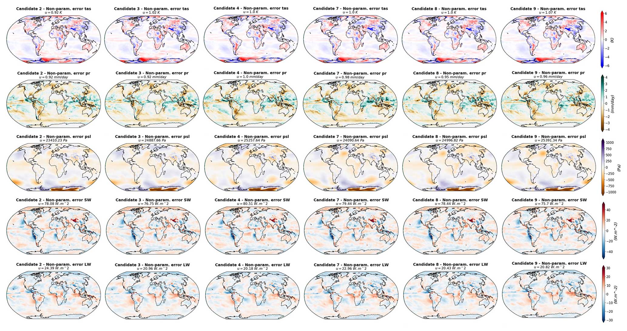
Figure E3 Non-parametric model errors in the second sub-set of candidates. Same as Fig. 10 for additional candidates.