the Creative Commons Attribution 4.0 License.
the Creative Commons Attribution 4.0 License.
 | 12 Jul 2024
AMOC stability amid tipping ice sheets: the crucial role of rate and noise
Peter Ashwin
Anna S. von der Heydt
Henk A. Dijkstra
The Atlantic Meridional Overturning Circulation (AMOC) has recently been categorized as a core tipping element as, under climate change, it is believed to be prone to critical transition implying drastic consequences on a planetary scale. Moreover, the AMOC is strongly coupled to polar ice sheets via meltwater fluxes. On the one hand, most studies agree on the fact that a collapse of the Greenland Ice Sheet would result in a weakening of AMOC. On the other hand, the consequences of a collapse of the West Antarctica Ice Sheet are less well understood. However, some studies suggest that meltwater originating from the Southern Hemisphere is able to stabilize the AMOC. Using a conceptual model of the AMOC and a minimal parameterization of ice sheet collapse, we investigate the origin and relevance of this stabilization effect in both the deterministic and stochastic cases. While a substantial stabilization is found in both cases, we find that rate- and noise-induced effects have substantial impact on the AMOC stability, as those imply that leaving the AMOC bistable regime is neither necessary nor sufficient for the AMOC to tip. Also, we find that rate-induced effects tend to allow a stabilization of the AMOC in cases where the peak of the West Antarctica Ice Sheet meltwater flux occurs before the peak of the Greenland Ice Sheet meltwater flux.
- Article
(2642 KB) - Full-text XML
-
Supplement
(404 KB) - BibTeX
- EndNote


Several components of the Earth system might abruptly and/or irreversibly collapse under climate warming. These are known as tipping elements (Lenton et al., 2008), each associated with a tipping point – a critical value of forcing above which the system is going to collapse. In a recent assessment, Armstrong McKay et al. (2022) classified the Atlantic Meridional Overturning Circulation (AMOC), the Greenland Ice Sheet (GIS), and West Antarctica Ice Sheet (WAIS) as global core tipping elements, as the loss of any of those climate components would lead to severe consequences on a planetary scale. There, it was also suggested that those three tipping elements might be at risk within the Paris Agreement warming range, while both polar ice sheets might already have crossed their critical threshold of global warming. Furthermore, an ongoing destabilization is in general supported by observations (see Caesar et al., 2018, for the AMOC; Shepherd et al., 2018, for the WAIS; and Shepherd et al., 2020, for the GIS) or studies based on early-warning signals (see Boers, 2021, Michel et al., 2022, Ditlevsen and Ditlevsen, 2023, and van Westen et al., 2024, for the AMOC; Rosier et al., 2021, for the WAIS; and Boers and Rypdal, 2021, for the GIS).
From a theoretical standpoint, tipping events are most often understood as the expression of a dynamic bifurcation intrinsic to the system. In this case, bifurcation-induced tipping can be avoided ensuring that external drivers (typically the global temperature) do not cross the critical value at which the bifurcation takes place. However, tipping events can also occur via inherently different processes, as described by Ashwin et al. (2012). On the one hand, those tipping events can be induced without crossing any critical value of external forcing and, in fact, without the presence of any bifurcation. Such tipping phenomena typically occur when the rate of variation in the external drivers is faster than the rate at which the system relaxes back to its attractor. The potential impact of those rate-induced tipping phenomena on the AMOC stability has been pointed out by numerous studies involving conceptual (Alkhayuon et al., 2019; Ritchie et al., 2023; Klose et al., 2024) or global ocean models (Lohmann and Ditlevsen, 2021). On the other hand, a tipping event can be triggered by the presence of stochastic noise, routinely used to represent the unresolved variability in the processes acting on a shorter timescale (Hasselmann, 1976; Frankignoul and Hasselmann, 1977). In this case, a system can collapse before crossing any critical value of forcing, solely due to the noise. In fact, noise-induced tipping phenomena potentially explain abrupt transitions observed in palaeoclimatic records known as Dansgaard–Oeschger events (Ditlevsen et al., 2007; Ditlevsen and Johnsen, 2010). The impact of noise on the AMOC stability has been investigated in a conceptual model by Castellana et al. (2019). There, the variability associated with the gradient of freshwater forcing over the Atlantic Ocean is able to induce a collapse of the overturning within the next century, with a probability estimated at about 15 %. In a later study, similar noise-induced tipping events have been shown to also occur in an ensemble of CMIP5 models (Castellana and Dijkstra, 2020).
As a further complication, the study of each tipping element individually might not suffice for producing reliable projections of tipping behaviour. Indeed, those elements are not isolated but may interact with each other, sometimes strongly, making it harder to predict the occurrence and severity of a tipping event. Arguably, the AMOC, GIS, and WAIS together form the most prominent example of such a coupled system of tipping elements. All three interact through various processes and on different timescales (Wunderling et al., 2021, 2024). On the one hand, a GIS collapse and the associated release of meltwater into the northern Atlantic Ocean is known to imply, at best, a weakening of the AMOC (Jackson and Wood, 2018; Bakker et al., 2016). On the other hand, a collapse of the AMOC could imply a warming of the Southern Hemisphere (Jackson et al., 2015; Stouffer et al., 2006), thereby accelerating ice loss in the WAIS (Favier et al., 2019; Joughin et al., 2014). Such a chain of destabilizing events is often referred to as cascading tipping or the domino effect (Dekker et al., 2018; Klose et al., 2021; Wunderling et al., 2021, 2024). However, this coupled system might also contain some stabilizing feedback. In this case, the collapse of one component may stabilize others, thereby making a global cascading event less likely. For example, using the state-of-the-art climate model HadGEM3, the collapse of the AMOC has been shown to imply a cooling of typically 5 to 8 °C over Greenland (Jackson et al., 2015), which would inhibit ice loss of the GIS.
A substantial source of uncertainty in how cascading tipping events could unfold lies in how a sudden ice loss from the WAIS would impact the AMOC. There, many different processes are at play and might either tend to destabilize it or keep it from collapsing (Swingedouw et al., 2009; Berk et al., 2021). In a conceptual model representing the AMOC and both polar ice sheets, Sinet et al. (2023) recently showed that the WAIS meltwater flux is able to prevent an AMOC collapse against the destabilization caused by both climate warming and ice loss from the GIS. In this study, the occurrence of an AMOC collapse drastically depends on the rate of forcing, as well as on the time delay between the tipping of both ice sheets. However, rate-induced effects were not explored in detail, and the stochastic case was not considered.
Motivated by the WAIS-induced stabilization effect on the AMOC found by Sinet et al. (2023), we explore its relevance in a more comprehensive conceptual model of the AMOC, considering also the stochastic case. For this, we perform a variety of model simulations using a simplified representation of tipping ice sheets. We aim to identify the distinct roles of rate-, noise-, and bifurcation-induced effects. The experimental setup is presented in Sect. 2. In Sect. 3, we reproduce a set of model simulations similar to Sinet et al. (2023), yielding a qualitatively similar AMOC stabilization effect of the WAIS meltwater flux. In Sect. 4, the bifurcation structure of the model is presented, allowing us to identify the presence of rate-induced effects. The robustness of this stabilization effect in the stochastic case is investigated in Sect. 5. Finally, a summary and a discussion are provided in Sect. 6.
In this section, we describe the conceptual model used to represent the AMOC and introduce a minimal representation of meltwater fluxes originating from the collapse of the GIS and WAIS.
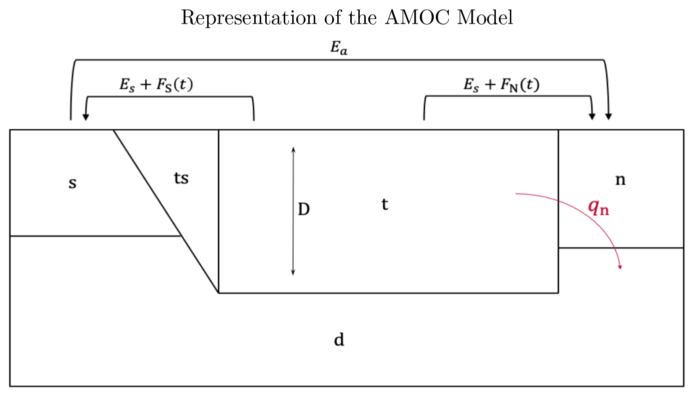
Figure 1The AMOC dynamics is captured by water transport between five distinct boxes, namely the Southern Ocean box (s), two thermocline boxes (t and ts), a deep-ocean box (d), and the northern Atlantic box (n). Each individual salinity is allowed to vary, as well as the pycnocline depth D. The parameters Ea and Es, denoting the asymmetric and symmetric component of the surface freshwater flux, respectively, are chosen to initialize the AMOC in an ON state (i.e. with strictly positive overturning strength qn). Meltwater fluxes FN,S(t) are added to the northern and southern box, respectively, and compensated for via evaporation at the Equator.
The AMOC is represented using the model introduced by Cimatoribus et al. (2014). There, the Atlantic Ocean is divided into five different regions depicted by boxes having distinct salinity and whose volume are allowed to vary, depending on the pycnocline depth (see Fig. 1). This box model includes two thermocline boxes, t and ts, where the latter represents a region in which the isopycnal slopes are greater than in other parts of the thermocline and allows for computing the density gradient within the Atlantic basin. Furthermore, the model is forced via two surface freshwater fluxes, Es and Ea (represented through virtual salt fluxes). The former stands for the amount of evaporation occurring in the tropical region and equally redistributed to each pole, while the latter introduces a pole-to-pole gradient of freshwater forcing. Given a value of Es, Cimatoribus et al. (2014) have shown that this model can yield bistability within some interval of Ea. Within this interval, one branch of stable steady states corresponds to a present-day-like AMOC with downwelling of dense waters in the northern box, or positive overturning strength (qn>0), while the other corresponds to a ceased overturning, or vanishing overturning strength (qn=0). Hereafter, we call those, respectively, the “ON” and “OFF” states. For a more detailed description of the AMOC model and numerical methods, see Appendix A.
To mimic the meltwater flux originating from collapsing ice sheets, time-dependent meltwater fluxes FN,S(t) (also represented through virtual salt fluxes) are inserted in the northern and southern box, respectively, and compensated for via evaporation at the Equator (see Fig. 1). Those are assumed to yield a parabolic shape in time, as follows:
where t is the time (in years), and PN,S is the duration of the GIS and WAIS collapse (also in years), respectively. Given that the GIS collapse is always initiated at t=0, the parameter Δt is the time at which the WAIS collapse is initiated or the time delay between the initiation of those two tipping events (which can be both positive or negative). Also, the parameters m3 and m3 are the volumes of, respectively, the GIS and WAIS (as in Sinet et al., 2023; based on Morlighem et al., 2017, 2020). To account for the WAIS meltwater lost in the Pacific or Indian oceans, we consider only a quarter of the meltwater originating from the WAIS to reach the Atlantic Ocean, as in Sinet et al. (2023). An alternative representation of FS(t) will also be used, where the tipping delay Δt is replaced by the delay between the maxima of both meltwater fluxes given by , which is positive if the maximum of FS(t) occurs after the maximum of FN(t). In this case, Eq. (2) is replaced by
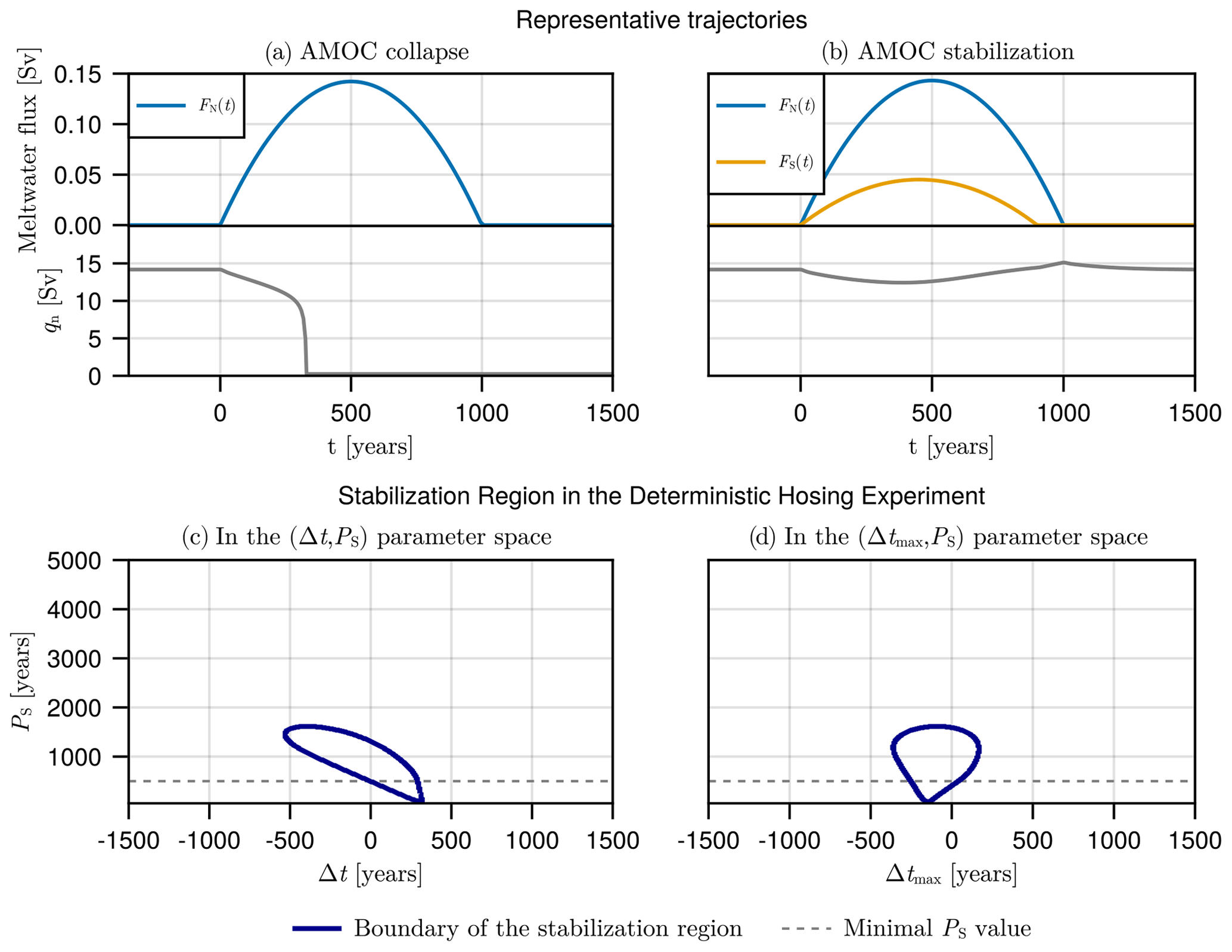
Figure 2(a–b) Representative trajectories of meltwater fluxes FN,S(t), as given by the set of Eqs. (1)–(2) (or Eqs. 1–3) and overturning strength qn. In panel (a), only a GIS collapse lasting PN=1000 years forces the AMOC model, resulting in an AMOC tipping (qn=0). In panel (b), both a GIS and a WAIS collapse force the AMOC model. Those last PN=1000 years and PS=900 years, respectively, and are initiated at the same time (Δt=0 years or, equivalently, years), resulting in an AMOC stabilization. (c–d) Boundary of the stabilization region in deterministic experiments involving both ice sheets, where the duration of the GIS collapse is fixed to PN=1000 years. Those are shown in panel (c) in the (Δt,PS) parameter space and in panel (d) in the (Δtmax,PS) parameter space. All parameter configurations within the stabilization region (dark blue curve) preserve the AMOC in an ON state (qn>0), while those outside lead the AMOC to an OFF state (qn=0). The dashed grey line represents the minimal value of the WAIS tipping duration at PS=500 years proposed by Armstrong McKay et al. (2022).
Hence, the forcing given by Eqs. (1)–(2) (or equivalently Eqs. 1–3) allows for conceptually capturing a full collapse of both ice sheets while spanning a wide range of possible tipping durations and delays, which is motivated by the uncertainty in ice sheet tipping points, tipping timescales, and global warming trajectories (Armstrong McKay et al., 2022), as well as the important role of those parameters found in Sinet et al. (2023). In the remainder of this document, we consider the interval [50,5000] years for the WAIS tipping duration PS, encompassing about the lower half of the interval [500,13 000] years proposed by Armstrong McKay et al. (2022). Also, to explore the impact of different ice sheet collapse trajectories, we use the delay interval years for both Δt and Δtmax.
In this section, we perform a set of model simulations to highlight the existence of a stabilizing impact of WAIS meltwater fluxes on the AMOC. For this, we initialize the AMOC in an ON state, choosing Ea=0.31 Sv. First, we investigate the situation in which only meltwater originating from the GIS is introduced in the Atlantic Ocean. In this case, the forcing is given by Eq. (1) alone and is fully determined by the parameter PN. We find that for PN≤1284 years, the AMOC ends in an OFF state. In the critical case of PN=1284 years, the OFF state is reached at about year 850 as the meltwater flux from the GIS amounts to approximately 0.10 Sv, consistent with typical forcing values leading the AMOC to a weak state in comprehensive models (Jackson and Wood, 2018).
To check whether stabilization effects associated with WAIS meltwater fluxes exist in this model, we force the AMOC with meltwater from both ice sheets. For this, we fix PN=1000 years given by Eq. (1) such that, by virtue of the previous experiment, the GIS forcing alone is sure to drive the AMOC to collapse. Indeed, using this value of PN, the OFF state is reached at about year 330, and the meltwater flux from the GIS reaches a maximal value of 0.14 Sv (see Fig. 2a). The WAIS melting trajectory is fully determined by either (Δt,PS) via Eq. (2) or (Δtmax,PS) via Eq. (3). The result of experiments involving meltwater fluxes from both ice sheets is represented in Fig. 2c in the (Δt,PS) parameter space and in Fig. 2d in the (Δtmax,PS) parameter space. We find a closed region in which the AMOC remains in an ON state (inside the dark blue boundary), hereafter called the stabilization region, while an OFF state was reached everywhere else (outside of the dark blue boundary). In particular, we find that the stabilization region exists for realistic values of the WAIS tipping duration PS (i.e. above the dashed grey line in Fig. 2c–d).
The existence of a stabilization region can be understood as explained in Cimatoribus et al. (2014). Given the sense of the circulation, meltwater inserted into the southern box implies a freshening of the box ts (see Fig. 1). This results in an increase in the density gradient between box ts and box n and hence an increase in the overturning strength qn (see Appendix A). However, in Fig. 2c, there appears to be an upper limit of the tipping delay at Δt≈320 years above which no stabilization can take place. Indeed, if no meltwater flux from the WAIS has already been applied by this time, then the AMOC is already engaged in its collapse. Also, the overall shape of the stabilization region indicates that, to result in an efficient stabilization of the AMOC, a longer WAIS collapse has to happen earlier than a shorter one. In a different experimental setup, these results qualitatively agree with those in Sinet et al. (2023). In both Fig. 2c and d, there is an upper limit of WAIS tipping duration at PS≈1600 years, above which FS(t) does not reach sufficiently high values to compensate for the comparatively strong GIS meltwater flux. Finally, in Fig. 2d, the approximate symmetry of the stabilization region suggests the existence of a negative optimal value of years. This value is optimal in the sense that the range of PS values for which a stabilization occurs shrinks as Δtmax moves away from it until the border of the stabilization region is reached. In other words, stabilization is most likely if the maximum of the WAIS meltwater flux occurs about 150 years before the maximum of the GIS meltwater flux.
Those results can be interpreted in the context of future climate change. In Armstrong McKay et al. (2022), plausible values for the GIS tipping duration PN are given in the range [1000,15 000] years, with a most likely value of 10 000 years. In our model, this most likely scenario results in the AMOC remaining stable regardless of the applied WAIS meltwater flux. Instead, PN=1000 years can be thought of as a worst-case scenario. This is further motivated by the modelling study of Aschwanden et al. (2019) in which a GIS collapsing on the millennial timescale was found under a RCP8.5 scenario. Under such conditions, the whole range of plausible WAIS tipping points of [1.5, 3.0] °C of global warming above pre-industrial levels (Armstrong McKay et al., 2022) would be overshot in less than a century, resulting in a negligible value of the time delay between ice sheet tipping events (Δt≈0 years). Hence, in such a worst-case scenario, a stabilization would occur for values of PS between approximately 500 and 1300 years (see the representative trajectory in Fig. 2b).
To gain a better understanding of the stabilization effect found in Fig. 2, we inspect the bifurcation structure of the AMOC model computed via numerical continuation using the Julia package BifurcationKit.jl (Veltz, 2020). In Fig. 3a, steady states of the model are shown in terms of the overturning strength qn versus positive values of the meltwater flux in the northern box FN. Those have been computed for three different values of FS=0.00, 0.04 and 0.08 Sv, yielding three distinct curves (with FS increasing from darker to lighter). In each case, bistability is observed within some interval of FN, above which the branch of stable present-day-like AMOC ceases to exist, while the collapsed AMOC configuration (qn=0) is always stable. This is sufficient to infer the existence of a bifurcation-induced tipping point, implying the potential of a critical transition as FN exceeds it. Via a similar approach, we also find that the sensitivity of the overturning strength qn to WAIS meltwater fluxes in the reference ON state is higher but comparable to what was found in Li et al. (2023) when using the coupled climate model GISS-E2.1-G (see Supplement Sect. S1). We note the presence of Hopf bifurcations, which move along the unstable branch as FS increases, and a Bogdanov–Takens bifurcation creating a new Hopf bifurcation on the stable branch, which keeps close to the saddle node bifurcation observed for each value of FS (see Fig. 3b). However, in terms of how the southern meltwater flux impacts the stability landscape, the most important general feature observed here is the expansion of the bistable region to higher values of FN when FS increases. This can in principle explain the stabilization effect taking place in previous experiments, as the tipping point of the AMOC becomes harder to reach.
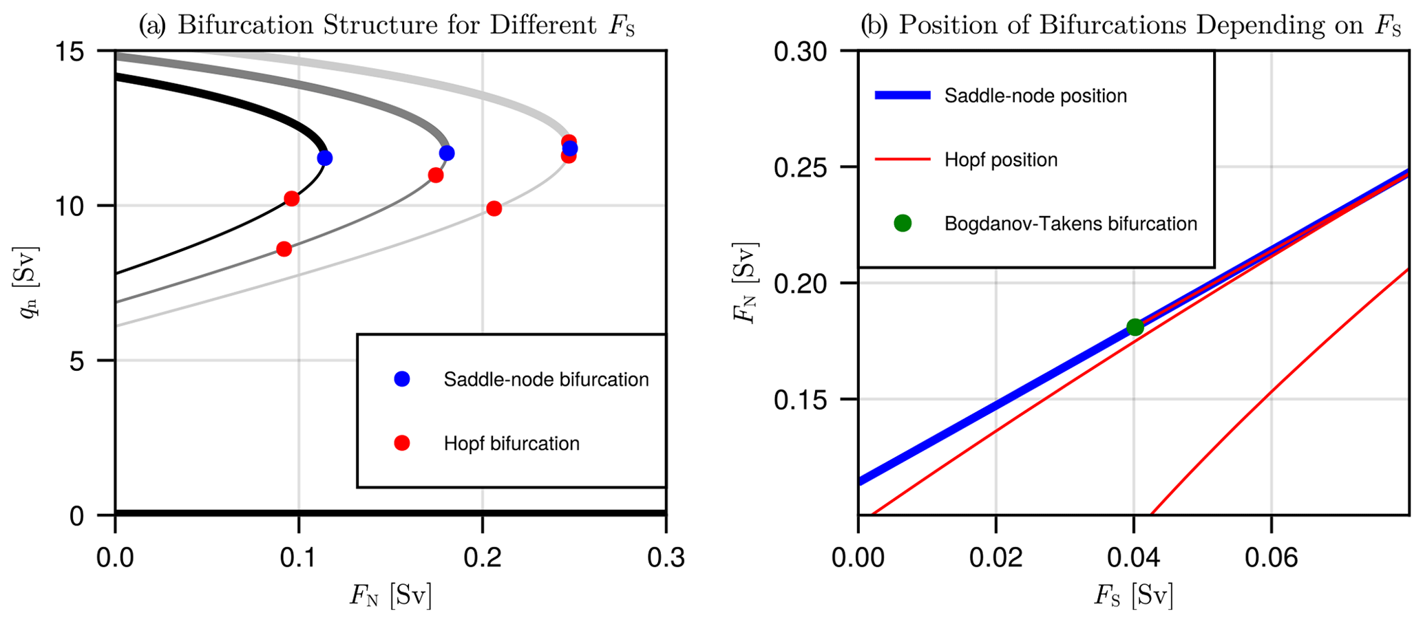
Figure 3(a) Bifurcation structure of the AMOC model in the (qn,FN) space. Thicker branches stand for stable steady states, while thinner branches indicate unstable steady states, and bifurcations are denoted by coloured points. The bifurcation structure has been computed for three different values of , and 0.08 (darker to lighter). (b) Displacement of bifurcations as FS varies. To the right of the Bogdanov–Takens bifurcation (green), a new Hopf bifurcation is created (in red; superposed to the saddle node bifurcation).
The value of FN at which the bistable region ends is approximately proportional to FS, with a proportionality coefficient δ approximately given by 1.68 (Fig. 3b). Noting that the bistable region ends at Sv in the case where FS=0.00 Sv, it is possible to identify meltwater flux trajectories that never lead the AMOC outside of its bistable region. That is, those satisfy
for all t∈ℝ. Given a fixed value of PN, these form a closed and compact region in the (Δt,PS) and (Δtmax,PS) parameter space for which the mathematical expression is given in Appendix B. Hence, fixing PN=1000 years as in the experiment represented in Fig. 2c–d, we can identify all parameter values for which no tipping point is ever overshot, hereafter called the no-overshoot region. In Fig. 4a–b, the limits of the no-overshoot region are drawn in red, and the boundary of the stabilization region found in Fig. 2 is drawn in dark blue. We find that these regions do not coincide, meaning that the AMOC stability cannot be predicted based on its bifurcation structure. In particular, we find that a collapse of the AMOC can happen inside the no-overshoot region (for parameter configurations within the red contour but outside of the dark blue contour). In this case, the AMOC reaches an OFF state without ever leaving its bistable region. Also, we find that an AMOC tipping avoidance (i.e. a stabilization) can occur even in some cases where the tipping point is overshot (for parameter configurations within the dark blue contour but outside of the red contour), a phenomena known as safe overshoot (Ritchie et al., 2021). Those are rate-induced effects, resulting in rate-induced tipping (Ashwin et al., 2012) or tipping avoidance (Ritchie et al., 2023), respectively.
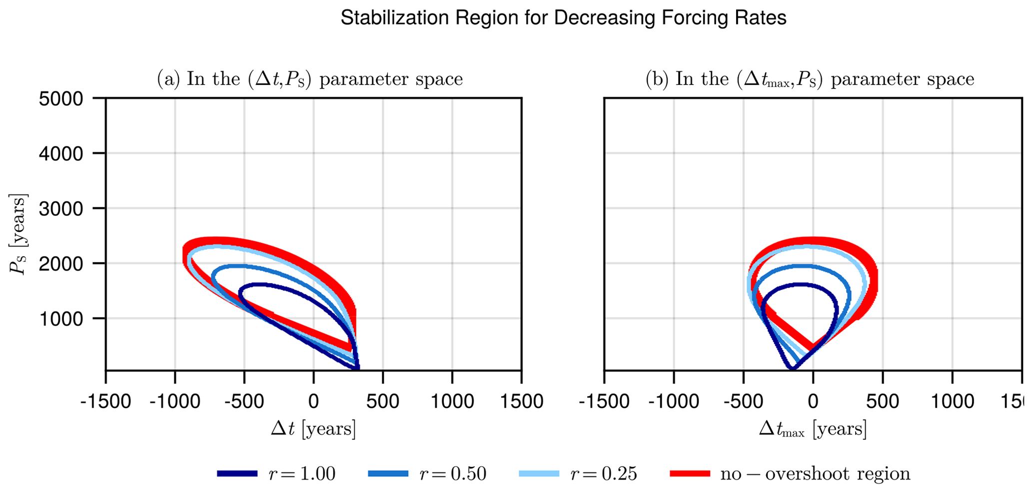
Figure 4Boundary of the no-overshoot region (in red) and the stabilization region computed for different values of the rate parameter r (nuances of blue), drawn in panel (a) in the (Δt,PS) parameter space and panel (b) in the (Δtmax,PS) parameter space. The darker blue contour (r=1) is the same as the one presented in Fig. 2c–d, while lighter blue contours correspond to lower values of r=0.50 and 0.25.
Rate-induced effects are less pronounced as the rate at which the forcing varies is decreased. This can be tested via artificially expanding the forcing timescale, using FN,S(rt) rather than FN,S(t) in the experiments. This has the effect of multiplying durations and delays by the inverse of the rate parameter r. In other words, the rate of variation in the forcing decreases as r decreases. For values of r lower than one, we stray away from reality as bigger volumes of meltwater are inserted in the Atlantic Ocean, but the bifurcation structure of the AMOC model under constant forcing remains unchanged, as well as the shape of the no-overshoot region. In Fig. 4a–b, we represent the boundary of the stabilization region in the same experiment using r=0.50 and 0.25 (lighter tones of blue). As expected, we find that the no-overshoot region (delimited by the red curve) gradually becomes a better approximation of the stabilization region, translating into a suppression of rate-induced effects. This results in transitions that are more consistent with the bifurcation-induced tipping case. Finally, we explain the approximate symmetry of the stabilization region in the (Δtmax,PS) parameter space found in Fig. 2d. The no-overshoot region (bounded by the red curve in Fig. 4b) is perfectly symmetric around Δtmax=0, which can also be directly inferred from its mathematical expression (see Appendix B). Hence, in the limit where r reaches zero, Δtmax=0 is the optimal value to result in a stabilization. While it is clear that the symmetry is broken as the value of r increases to one, the stabilization region still preserves some degree of symmetry around some optimal, negative value of Δtmax. In other words, the (negative) optimal value of Δtmax depends on the rate of forcing.
The importance of rate-induced effects in this model can be explained by the fact that trajectories are relatively slowly attracted to the stable attractor. As an illustration, we note that the previously found critical value of the GIS tipping duration at PN=1284 years in Sect. 3 does not result in an overshoot of the tipping point. In this case, performing the same simulation with decreased r results in the AMOC never reaching the OFF state (as shown in Fig. 5a). This originates from the slow timescale induced by the dynamics of the pycnocline depth D. In fact, the decay time towards the stable equilibrium can be computed as the inverse of the least negative eigenvalue of the associated stable state which, as shown in Fig. 5b, is always above 190 years. This slow timescale can be connected to the pycnocline depth by computing the associated eigenvector, in which we find that the direction corresponding to the pycnocline depth D dominates the others by approximately a factor 100. This indicates that, for the values of PN considered, the separation between the forcing timescale and the decay timescale toward stable equilibria (driven by the dynamics of the pycnocline depth) is not large enough to prevent rate-induced effects.
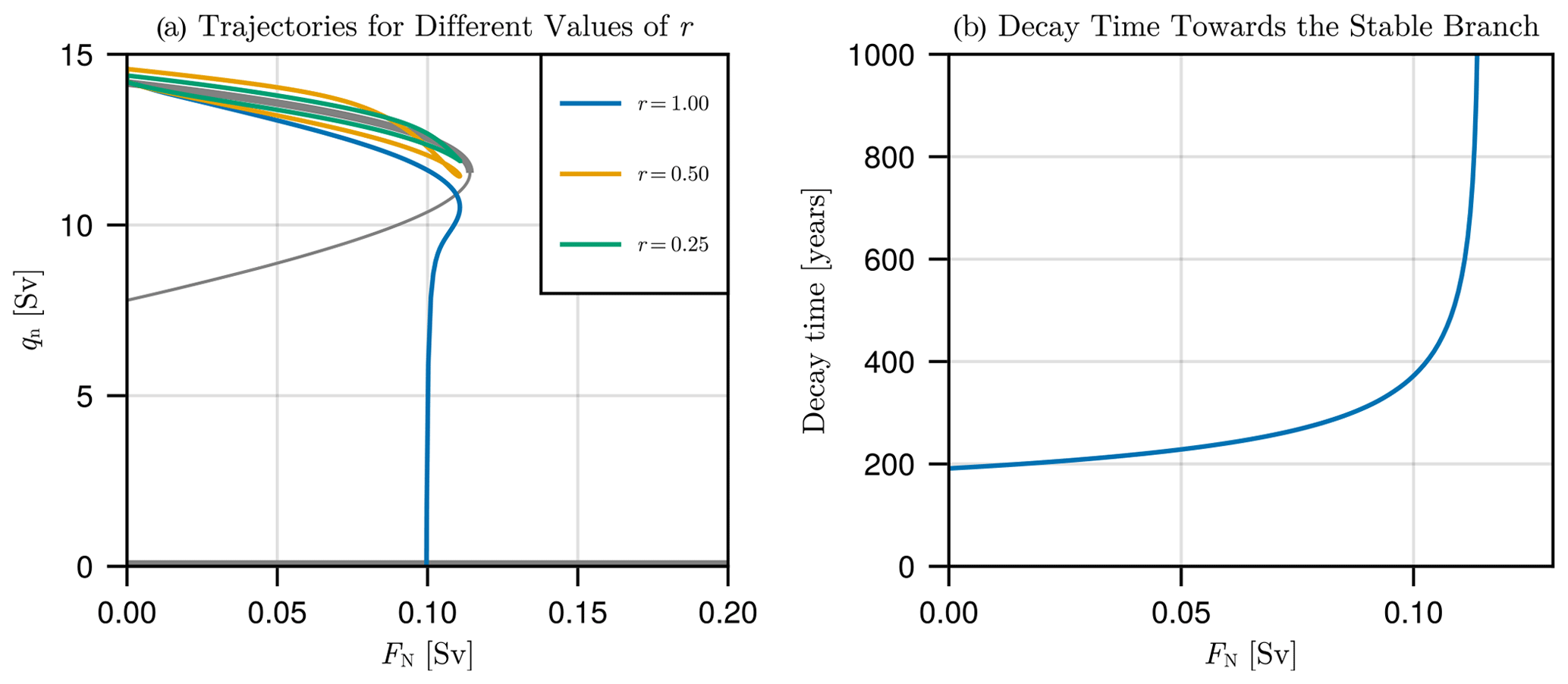
Figure 5(a) Trajectories in the experiment where only the GIS meltwater flux forces the AMOC via Eq. (1) using PN=1284 years and represented in the (qn,FN) space for different values of the rate parameter r=1.00, 0.50, and 0.25. Steady states for fixed FN are added in grey, where thicker lines stand for the stable states. (b) Variation in the decay time along the upper stable branch. The minimum is for FN=0.00 at about 190 years.
In this section, we evaluate the relevance of the stabilization effect of WAIS meltwater fluxes on the AMOC when natural variability is added to the surface freshwater flux. To do so, we redefine the asymmetric component of the surface freshwater flux Ea in the following way (Castellana et al., 2019; Jacques-Dumas et al., 2023):
Here, is a constant representing the mean value of the asymmetric component of the surface freshwater flux, ξ(t) is a white noise process with zero mean and unit variance, and fσ is the noise strength parameter. As found by Castellana et al. (2019), a non-zero value of fσ renders noise-induced tipping possible, where the AMOC can reach an OFF state solely due to the noise, independently of any meltwater forcing. From this point of view, both the cases in which the tipping point of the AMOC model can be overshot or not are relevant and will be considered. To choose the noise strength parameter fσ, we note that, at the value (which we choose analogously to the deterministic case), Castellana et al. (2019) showed that results in the AMOC reaching an OFF state within 100 years with a probability of at least one-third. In our case, as we are interested in millennial timescales, such noise strengths would lead the AMOC to collapse almost surely, regardless of the applied meltwater fluxes in any experiment. For a better signal-to-noise ratio, we choose to use a weaker noise by setting fσ=0.05. Finally, to be able to later compare transition probabilities in the same (Δt,PS) and (Δtmax,PS) parameter spaces as before, we must ensure that white noise takes effect at the same given time in every simulation. Hence, we will systematically start numerical integration at year −3500, corresponding to the minimal time at which the WAIS tipping is initiated. In the remainder of this section, transition probabilities are computed via Monte Carlo sampling, using 10 000 trajectories.
First, we focus on transition probabilities when only the GIS meltwater flux forces the AMOC via Eq. (1). This is performed for two distinct values of PN=1000 and 2000 years, where the former leads to an overshoot of the AMOC tipping point, while the latter does not. In Fig. 6, we show the time evolution of the cumulative transition probability pGIS(t), which stands for the probability that the AMOC transitions to an OFF state before time t. We observe that before the GIS collapse (t<0), this probability increases almost linearly in time, solely due to the noise. From the moment that the GIS collapse is initiated (t=0), the probability sharply increases as the value of FN(t) brings the trajectory closer (or past) the border of the bistable region. This happens in both the cases where overshoot of the AMOC tipping point occurs or not; although, in the case of PN=2000 years, the probability increases at a milder rate than for PN=1000 years.

Figure 6Time evolution of the cumulative probability of AMOC transition pGIS(t) for PN=1000 (blue) and 2000 (yellow) years, using fσ=0.05 in both cases. Vertical dotted lines represent the three different times considered in Fig. 7. Probabilities were computed via Monte Carlo sampling for 10 000 trajectories.
Second, using the same values of PN, we force the AMOC model with the full condition given by Eqs. (1)–(2) (or Eqs. 1–3). Integrating the system in time, this leads to a new cumulative probability of AMOC transition pGIS,WAIS(t), interpreted in the same manner as pGIS(t). To assess the magnitude of any stabilization effect originating from the WAIS meltwater flux, we use the following metric:
hereafter called relative probability change. It represents the percentage by which the cumulative transition probability varies with respect to the situation in which the GIS alone forces the AMOC. In other words, at any given time t, a negative value of δp(t) indicates a stabilization induced by the WAIS collapse.
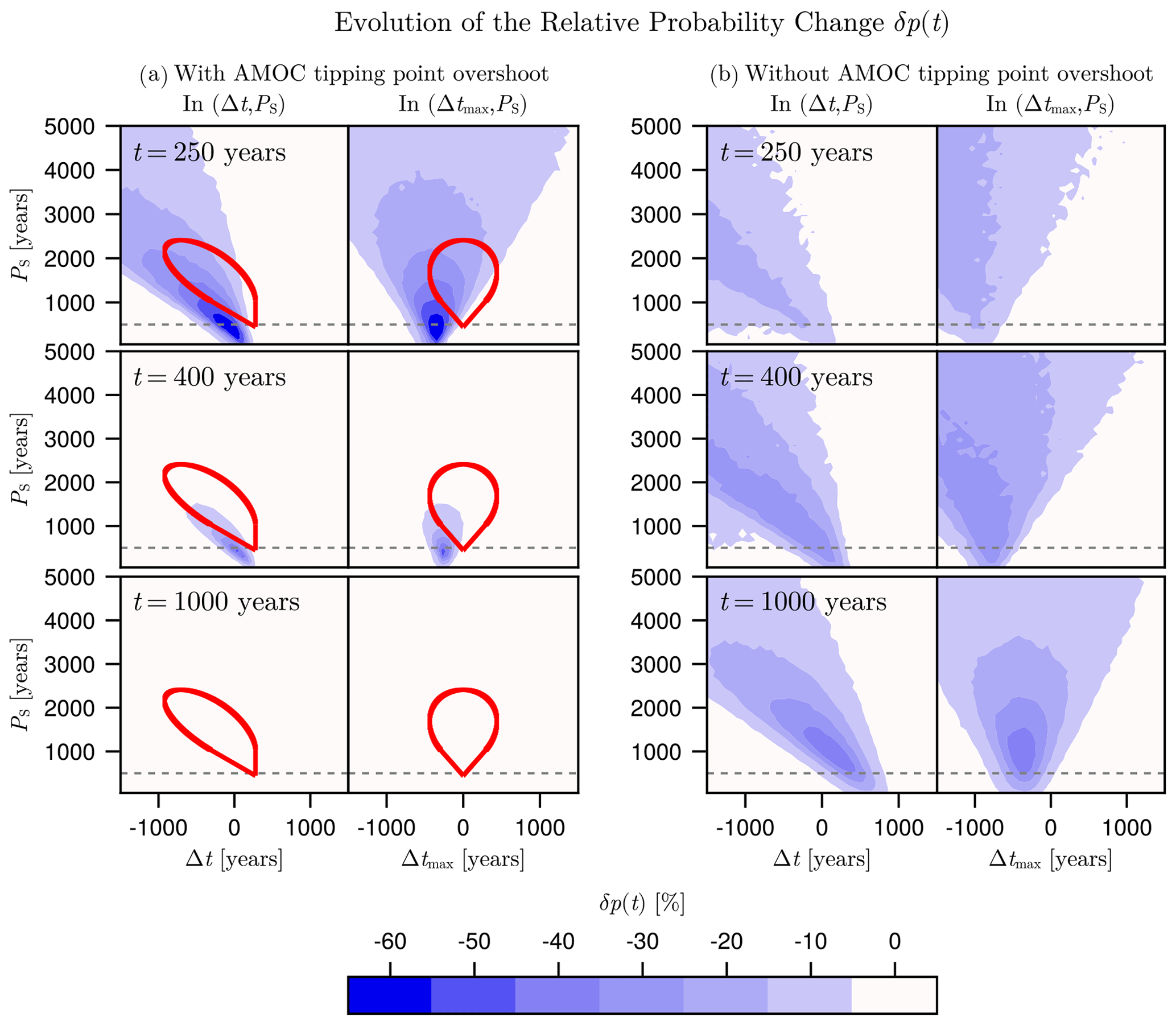
Figure 7Evolution of the relative probability change δp(t) (defined by Eq. 6) in stochastic experiments using fσ=0.05. We use (a) PN=1000 years, in which case the tipping point of the AMOC is overshot outside of the no-overshoot region (bounded by the red curve), and (b) PN=2000 years, in which case the tipping point of the AMOC is never overshot. For both panels (a) and (b), results are drawn in the (Δt,PS) parameter space (left column) and in the (Δtmax,PS) parameter space (right column) at three different times, namely , and 1000 years (top to bottom). The dashed grey line represents the minimal value of the WAIS tipping duration at PS=500 years, as proposed by Armstrong McKay et al. (2022). Each probability has been computed via Monte Carlo sampling, using 10 000 trajectories.
In Fig. 7a, PN=1000 years was used, such that the AMOC tipping point is to be overshot everywhere except in the no-overshoot region (bounded by the red curve). The relative probability change is represented in both the (Δt,PS) parameter space (left column) and the (Δtmax,PS) parameter spaces (right column) at three different times, namely at years 250, 400, and 1000 (top to bottom; also drawn as dotted vertical lines in Fig. 6). At year 250, δp reaches −63 %. While the overshoot of the AMOC tipping point has not occurred yet (and does not before year 280), it is interesting to note that the regions of the strongest probability decrease are consistent in shape with the no-overshoot region in both parameter spaces, although with a clear shift, which will be discussed at the end of this section. At year 400, only a small region of lower probability remains and gradually disappears as time increases, as can be seen at year 1000, where δp is uniformly close to zero. Results of the experiment using PN=2000 years, meaning that there is no region in the (Δt,PS) parameter space where the AMOC tipping point is ever overshot, are presented in Fig. 7b. In this case, δp at year 250 is already substantially negative in a wide region of the parameter space and even more so at year 400. Importantly, we see that the stabilization is still present and substantial on longer timescales, as seen at year 1000. It is also interesting to note that the region of the strongest probability decrease gradually becomes similar in shape to the previously found no-overshoot region as, here, no overshoot can occur. However, as t increases, the centre of this region clearly shifts toward higher values of Δtmax. This also happens in the case of PN=1000 years (Fig. 7a), although less clearly. In summary, we find that the relative probability change can be substantially negative in both the case when an AMOC overshoot can occur or not. This probability decrease occurs for realistic values of the WAIS tipping duration PS (i.e. above the dashed grey line in Fig. 7a–b). However, varying the forcing rate yields important quantitative differences in the magnitude of this stabilization effect and on its specific timescale.
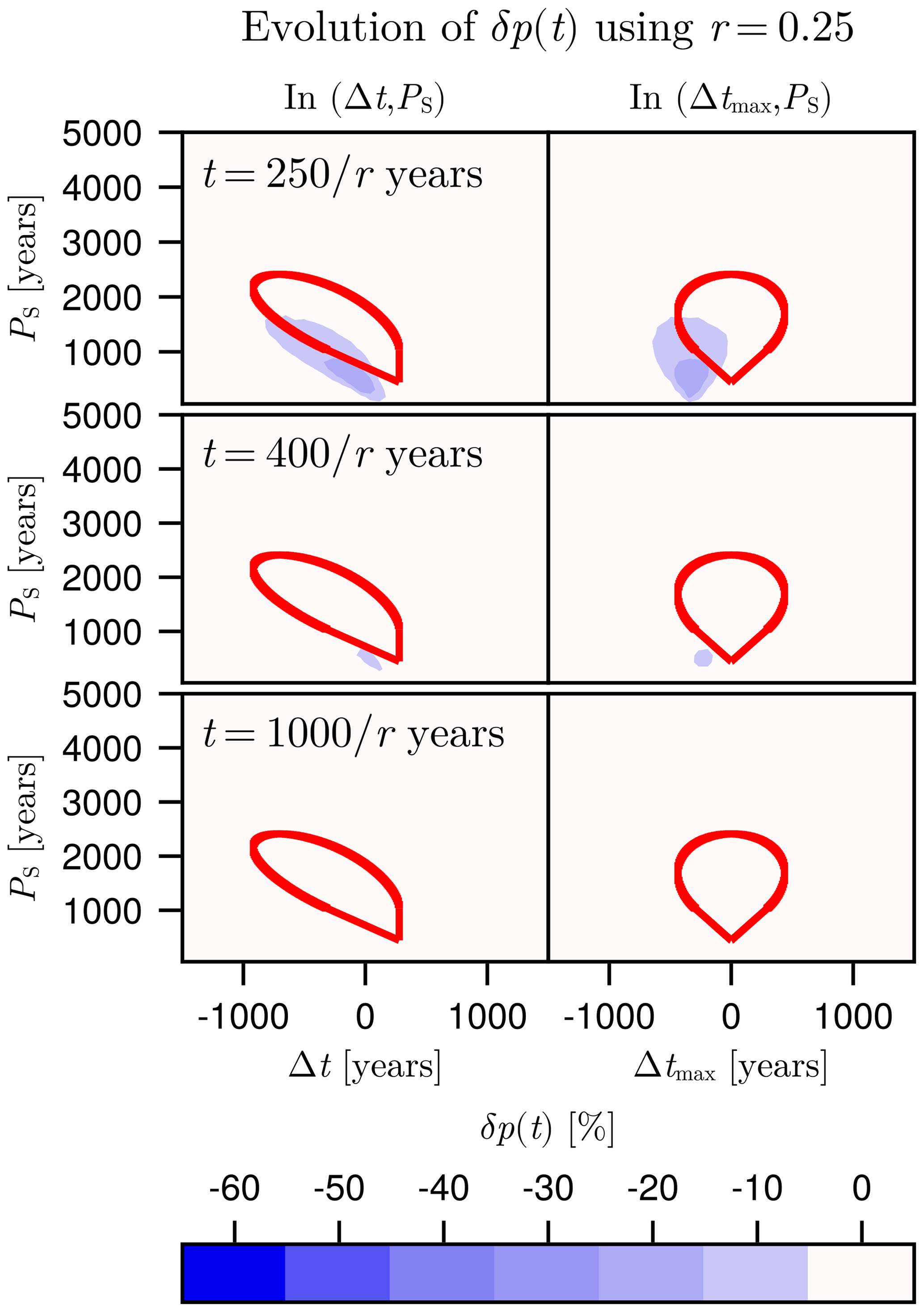
In Fig. 7a, we found that the regions of strongest probability change and the no-overshoot region are similar in shape but not in location. Analogous to the results of Sect. 4, it is tempting to also relate this shift to rate-induced effects. This can be verified by performing similar stochastic experiments for a lower value of the rate parameter r (used as in Sect. 4). In Fig. 8, we show the results obtained using PN=1000 years and r=0.25. Again, to present results in the same (Δt,PS) and (Δtmax,PS) parameter space, we ensure that the noise is added at the same time in all experiments by starting the integration at years. Hence, quantitative differences with respect to Fig. 7a can be related to the fact that white noise acts during a much longer time, while the region in which δp is most negative remains similar. Most importantly, we find that the no-overshoot region does not become a better approximation of the region of the strongest probability decrease at any time, despite the low value used for the rate parameter r. This implies that the shift between the no-overshoot region and the region in which δp is most negative cannot be explained (only) by rate-induced effects but clearly involves noise-induced effects.
In this study, the stability of the AMOC was explored in numerical simulations involving meltwater fluxes from both polar ice sheets. Although in a different experimental setup, the same qualitative results of Sinet et al. (2023) were verified, where the occurrence of an AMOC tipping depends on the timescale of both ice sheet collapses and the delay between those collapses. In a worst-case scenario where the GIS fully collapses in 1000 years (as suggested by Armstrong McKay et al., 2022), deterministic results of Sect. 3 indicated that a stabilizing influence of the WAIS collapse is strong enough to stabilize the AMOC. Notably, this stabilization can occur for a relatively fast WAIS collapse lasting up to 1600 years, corresponding to the lower projections of WAIS tipping durations (Armstrong McKay et al., 2022). Regarding the AMOC stabilization, the use of two different parameterizations of WAIS tipping trajectories informed us on the existence of some optimal scenario for the tipping of ice sheets, where the peak of WAIS meltwater flux occurs about 150 years before the peak of GIS meltwater flux.
In Sect. 4, a detailed investigation of the AMOC bifurcation structure allowed us to identify the no-overshoot region in the forcing parameter space, defining WAIS tipping scenarios for which the tipping point of the AMOC is never reached. This revealed that an AMOC collapse could be induced without leaving the bistable regime at any time, as well as the existence of safe-overshoot trajectories. Such rate-induced effects occur when ice sheets collapse on a timescale which is comparable to the recovery timescale of the AMOC, whose high value originates from the slow dynamics of the pycnocline depth. The existence of those rate-induced effects was confirmed by artificially slowing down the rate of variation in meltwater input, yielding results that became more consistent with bifurcation-induced critical transitions. This analysis allows us to find that the previously found optimal delay between the peaks of both meltwater fluxes is highly rate-dependent.
Under stochastic noise in the surface freshwater flux (Sect. 5), the stabilization effect of WAIS meltwater fluxes remains important. In contrast to the deterministic context (Sect. 3), a drastic decrease in the AMOC transition probability is now possible in the case of slower WAIS collapse of up to 5000 years, spanning about the lower half of the range of WAIS tipping durations suggested by Armstrong McKay et al. (2022). On the one hand, we investigated the worst-case scenario in which the GIS fully collapses in 1000 years, such that an overshoot of the AMOC tipping point can occur. In this case, we found that some WAIS trajectories result in a substantial decrease in the cumulative AMOC tipping probability (of up −63 %), although remaining important only on the centennial timescale. On the other hand, we considered cases implying a comparatively slower GIS tipping lasting 2000 years, such that the tipping point of the AMOC is never overshot. In this case, we found that a similar probability decrease can persist way longer in time, on the millennial timescale. Finally, we were able to demonstrate that, due to noise-induced effects, ice sheet tipping scenarios yielding the strongest stabilization cannot be accurately predicted by bifurcation analysis. Yet, similarities between the region of strongest stabilization and the no-overshoot region motivate further investigation via the tools of stochastic dynamics (e.g. as in Berglund and Gentz, 2006).
Clearly, the scope of our results is limited by the conceptual nature of the model used, as was the case in Sinet et al. (2023). On the one hand, ice sheet melting trajectories were purposefully chosen to be minimalist, and important processes were omitted. First, the cooling of the northern polar region induced by an AMOC weakening (Jackson et al., 2015; van Westen et al., 2024) was not included and may render the AMOC tipping less likely via inhibition of a GIS collapsing. Second, the warming of the Southern Hemisphere subsequent to an AMOC weakening (Jackson et al., 2015; Stouffer et al., 2006) was not considered and could result in a WAIS collapse on a faster timescale. This could imply a shift in the time delay between the peak of both ice sheet meltwater fluxes towards negative values, thus either pushing this delay closer to or further away from its optimal value for a stabilization event to occur. On the other hand, only part of the AMOC dynamics is represented in a box model. In a more detailed setup, our quantitative results regarding rate- and noise-induced effects would most likely be challenged and vary among different models. Indeed, comprehensive models display an important range of sensitivities to northern (Jackson et al., 2023) and southern (Swart et al., 2023) freshwater fluxes. Furthermore, the AMOC tipping point varies substantially in different Earth system Models of Intermediate Complexity (EMICs) (Rahmstorf et al., 2005) and was only recently found in a global climate model (van Westen and Dijkstra, 2023). A direct extension of this study would be to investigate how the results compare to those obtained in EMICs which, as in our case, can be obtained using only prescribed meltwater fluxes.
Nonetheless, the existence of such important rate- and noise-induced effects at the conceptual level informs us on the limits of an analysis focused solely on bifurcation-induced transitions. It suggests that maintaining meltwater fluxes under some critical value might not suffice for ensuring the AMOC stability. Yet, the significant stabilizing impact of a WAIS collapse on the AMOC stability, as found in Sinet et al. (2023), is consistently found in a different conceptual AMOC model and motivates further investigation. Finally, the decisive role of forcing rates encourages efforts to produce accurate predictions of ice sheet melting under future global warming.
The conceptual AMOC model represents the Atlantic Ocean as five distinct boxes (see Fig. 1) of constant temperature but time-varying salinity and includes a dynamical representation of the pycnocline depth. The time evolution of salinities Si for and the pycnocline depth D are given by differential equations identical to those used earlier (Cimatoribus et al., 2014; Castellana et al., 2019; Jacques-Dumas et al., 2023), except for the addition of time-dependent meltwater fluxes FN,S(t) defined by Eqs. (1)–(2) (or Eqs. 1–3), as follows:
where θ(x) stands for the Heaviside function. Those include wind-driven transports rs,n originating from sub-tropical gyres and the following volume transports:
where densities ρi for are given by
and volumes are given by
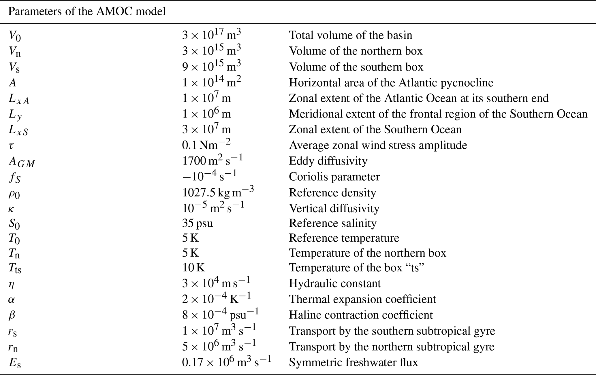
The different constants used in the model are provided in Table A1. Throughout the study, numerical time integration is performed using the Julia package DifferentialEquations.jl (Rackauckas and Nie, 2017). The Runge–Kutta algorithm of order 4 is used for integration of the deterministic model, while the SOSRI algorithm (best described in Rackauckas and Nie, 2020) is used for integration of the stochastic model. Finally, the Julia package BifurcationKit.jl (Veltz, 2020) is used for numerical continuation.
As justified in Sect. 4, meltwater forcing trajectories will never bring the AMOC model outside of its bistable region if the condition given by Eq. (4) is verified for all t∈ℝ. Given a set value of PN>0, such trajectories (if they exist) are found in the (Δt,PS) and (Δtmax,PS) parameter spaces by analysis, thus yielding the no-overshoot region. In what follows, computations are performed in the (Δtmax,PS) parameter space. We begin by noting that FN(t) overshoots the critical value FN,c if and only if
otherwise, the condition given by Eq. (4) is trivially verified in all cases. In the case where Eq. (B1) holds, the overshoot occurs during the interval , where
and
Now, by virtue of the positivity of FS(t), a necessary condition for the condition given by Eq. (4) to be satisfied is that FS(t) does not vanish for any t in . In other words, must be fully contained in , which is true if and only if
In this case, it remains only to ensure that the second-degree polynomial,
does not overshoot zero within the time interval . Again, by virtue of the positivity of FS(t), this is true if and only if one of the three following criteria holds:
-
is always positive or zero. This implies that G(t) is majored by zero within and is true if and only if
-
is always strictly negative, but G(t) does not overshoot zero for any value of t. It is true if and only if the discriminant of G(t) is negative or zero, translating into
-
is always strictly negative and G(t) overshoots zero but only in a finite region outside of . This is equivalent to requiring that the maximum of G(t) is found outside of , which is true if and only if
To summarize, given a set value of PN>0 for which FN(t) overshoots FN,c (meaning that the condition given by Eq. B1 holds), forcing trajectories verifying the condition given by Eq. (4) may exist. Those verify Eq. (B4), along with either criteria given by Eq. (B7), Eq. (B8), or Eq. (B9). We note that, as all those conditions are invariant under the transformation , the no-overshoot region yields an axial symmetry around Δtmax=0. Finally, this region can be described in the (Δt,PS) parameter space, simply by substituting in each condition.
The supplement related to this article is available online at: https://doi.org/10.5194/esd-15-859-2024-supplement.
SS carried out the analysis and drafted the paper. PA, ASvdH, and HAD advised on the study. All authors contributed to the submitted paper.
The contact author has declared that none of the authors has any competing interests.
Publisher’s note: Copernicus Publications remains neutral with regard to jurisdictional claims made in the text, published maps, institutional affiliations, or any other geographical representation in this paper. While Copernicus Publications makes every effort to include appropriate place names, the final responsibility lies with the authors.
This article is part of the special issue “Tipping points in the Anthropocene”. It is a result of the “Tipping Points: From Climate Crisis to Positive Transformation” international conference hosted by the Global Systems Institute (GSI) and University of Exeter (12–14 September 2022), as well as the associated creation of a Tipping Points Research Alliance by GSI and the Potsdam Institute for Climate Research, Exeter, Great Britain, 12–14 September 2022.
This project has received funding from the European Union's Horizon 2020 research and innovation programme under the Marie Skłodowska-Curie Actions (grant no. 956170; CriticalEarth). Anna S. von der Heydt acknowledges funding by the Dutch Research Council (NWO) through the NWO-Vici project “Interacting climate tipping elements: When does tipping cause tipping?” (project no. VI.C.202.081).
This paper was edited by Gabriele Messori and reviewed by two anonymous referees.
Alkhayuon, H., Ashwin, P., Jackson, L. C., Quinn, C., and Wood, R. A.: Basin bifurcations, oscillatory instability and rate-induced thresholds for Atlantic meridional overturning circulation in a global oceanic box model, Proc. Roy. Soc. A, 475, 20190051, https://doi.org/10.1098/rspa.2019.0051, 2019. a
Armstrong McKay, D. I., Staal, A., Abrams, J. F., Winkelmann, R., Sakschewski, B., Loriani, S., Fetzer, I., Cornell, S. E., Rockström, J., and Lenton, T. M.: Exceeding 1.5 °C global warming could trigger multiple climate tipping points, Science, 377, eabn7950, https://doi.org/10.1126/science.abn7950, 2022. a, b, c, d, e, f, g, h, i, j
Aschwanden, A., Fahnestock, M. A., Truffer, M., Brinkerhoff, D. J., Hock, R., Khroulev, C., Mottram, R., and Khan, S. A.: Contribution of the Greenland Ice Sheet to sea level over the next millennium, Sci. Adv., 5, eaav9396, https://doi.org/10.1126/sciadv.aav9396, 2019. a
Ashwin, P., Wieczorek, S., Vitolo, R., and Cox, P.: Tipping points in open systems: bifurcation, noise-induced and rate-dependent examples in the climate system, Philos. T. R. Soc. A, 370, 1166–1184, 2012. a, b
Bakker, P., Schmittner, A., Lenaerts, J. T. M., Abe-Ouchi, A., Bi, D., van den Broeke, M. R., Chan, W.-L., Hu, A., Beadling, R. L., Marsland, S. J., Mernild, S. H., Saenko, O. A., Swingedouw, D., Sullivan, A., and Yin, J.: Fate of the Atlantic Meridional Overturning Circulation: Strong decline under continued warming and Greenland melting, Geophys. Res. Lett., 43, 12252–12260, https://doi.org/10.1002/2016GL070457, 2016. a
Berglund, N. and Gentz, B.: Noise-Induced Phenomena in Slow-Fast Dynamical Systems: A Sample-Paths Approach, Probability and Its Applications, Springer London, ISBN 9781846281860, https://doi.org/10.1007/1-84628-186-5, 2006. a
Berk, J. v. d., Drijfhout, S. S., and Hazeleger, W.: Circulation adjustment in the Arctic and Atlantic in response to Greenland and Antarctic mass loss, Clim. Dynam., 57, 1689–1707, https://doi.org/10.1007/s00382-021-05755-3, 2021. a
Boers, N.: Observation-based early-warning signals for a collapse of the Atlantic Meridional Overturning Circulation, Nat. Clim. Change, 11, 680–688, https://doi.org/10.1038/s41558-021-01097-4, 2021. a
Boers, N. and Rypdal, M.: Critical slowing down suggests that the western Greenland Ice Sheet is close to a tipping point, P. Natl. Acad. Sci. USA, 118, e2024192118, https://doi.org/10.1073/pnas.2024192118, 2021. a
Caesar, L., Rahmstorf, S., Robinson, A., Feulner, G., and Saba, V.: Observed fingerprint of a weakening Atlantic Ocean overturning circulation, Nature, 556, 191–196, https://doi.org/10.1038/s41586-018-0006-5, 2018. a
Castellana, D. and Dijkstra, H. A.: Noise-induced transitions of the Atlantic Meridional Overturning Circulation in CMIP5 models, Sci. Rep., 10, 20040, https://doi.org/10.1038/s41598-020-76930-5, 2020. a
Castellana, D., Baars, S., Wubs, F. W., and Dijkstra, H. A.: Transition Probabilities of Noise-induced Transitions of the Atlantic Ocean Circulation, Sci. Rep., 9, 20284, https://doi.org/10.1038/s41598-019-56435-6, 2019. a, b, c, d, e
Cimatoribus, A. A., Drijfhout, S. S., and Dijkstra, H. A.: Meridional overturning circulation: stability and ocean feedbacks in a box model, Clim. Dynam., 42, 311–328, https://doi.org/10.1007/s00382-012-1576-9, 2014. a, b, c, d
Dekker, M. M., von der Heydt, A. S., and Dijkstra, H. A.: Cascading transitions in the climate system, Earth Syst. Dynam., 9, 1243–1260, https://doi.org/10.5194/esd-9-1243-2018, 2018. a
Ditlevsen, P. and Ditlevsen, S.: Warning of a forthcoming collapse of the Atlantic meridional overturning circulation, Nat. Commun., 14, 4254, https://doi.org/10.1038/s41467-023-39810-w, 2023. a
Ditlevsen, P. D. and Johnsen, S. J.: Tipping points: Early warning and wishful thinking, Geophys. Res. Lett., 37, L19703, https://doi.org/10.1029/2010GL044486, 2010. a
Ditlevsen, P. D., Andersen, K. K., and Svensson, A.: The DO-climate events are probably noise induced: statistical investigation of the claimed 1470 years cycle, Clim. Past, 3, 129–134, https://doi.org/10.5194/cp-3-129-2007, 2007. a
Favier, L., Jourdain, N. C., Jenkins, A., Merino, N., Durand, G., Gagliardini, O., Gillet-Chaulet, F., and Mathiot, P.: Assessment of sub-shelf melting parameterisations using the ocean–ice-sheet coupled model NEMO(v3.6)–Elmer/Ice(v8.3), Geosci. Model Dev., 12, 2255–2283, https://doi.org/10.5194/gmd-12-2255-2019, 2019. a
Frankignoul, C. and Hasselmann, K.: Stochastic climate models, Part II, Application to sea-surface temperature anomalies and thermocline variability, Tellus, 29, 289–305, https://doi.org/10.1111/j.2153-3490.1977.tb00740.x, 1977. a
Hasselmann, K.: Stochastic climate models Part I, Theory, Tellus, 28, 473–485, https://doi.org/10.1111/j.2153-3490.1976.tb00696.x, 1976. a
Jackson, L. C. and Wood, R. A.: Hysteresis and Resilience of the AMOC in an Eddy-Permitting GCM, Geophys. Res. Lett., 45, 8547–8556, https://doi.org/10.1029/2018GL078104, 2018. a, b
Jackson, L. C., Kahana, R., Graham, T., Ringer, M. A., Woollings, T., Mecking, J. V., and Wood, R. A.: Global and European climate impacts of a slowdown of the AMOC in a high resolution GCM, Clim. Dynam., 45, 3299–3316, https://doi.org/10.1007/s00382-015-2540-2, 2015. a, b, c, d
Jackson, L. C., Alastrué de Asenjo, E., Bellomo, K., Danabasoglu, G., Haak, H., Hu, A., Jungclaus, J., Lee, W., Meccia, V. L., Saenko, O., Shao, A., and Swingedouw, D.: Understanding AMOC stability: the North Atlantic Hosing Model Intercomparison Project, Geosci. Model Dev., 16, 1975–1995, https://doi.org/10.5194/gmd-16-1975-2023, 2023. a
Jacques-Dumas, V., van Westen, R. M., Bouchet, F., and Dijkstra, H. A.: Data-driven methods to estimate the committor function in conceptual ocean models, Nonlin. Processes Geophys., 30, 195–216, https://doi.org/10.5194/npg-30-195-2023, 2023. a, b
Joughin, I., Smith, B. E., and Medley, B.: Marine Ice Sheet Collapse Potentially Under Way for the Thwaites Glacier Basin, West Antarctica, Science, 344, 735–738, https://doi.org/10.1126/science.1249055, 2014. a
Klose, A. K., Wunderling, N., Winkelmann, R., and Donges, J. F.: What do we mean, “tipping cascade”?, Environ. Res. Lett., 16, 125011, https://doi.org/10.1088/1748-9326/ac3955, 2021. a
Klose, A. K., Donges, J. F., Feudel, U., and Winkelmann, R.: Rate-induced tipping cascades arising from interactions between the Greenland Ice Sheet and the Atlantic Meridional Overturning Circulation, Earth Syst. Dynam., 15, 635–652, https://doi.org/10.5194/esd-15-635-2024, 2024. a
Lenton, T. M., Held, H., Kriegler, E., Hall, J. W., Lucht, W., Rahmstorf, S., and Schellnhuber, H. J.: Tipping elements in the Earth's climate system, P. Natl. Acad. Sci. USA, 105, 1786–1793, https://doi.org/10.1073/pnas.0705414105, 2008. a
Li, Q., Marshall, J., Rye, C. D., Romanou, A., Rind, D., and Kelley, M.: Global Climate Impacts of Greenland and Antarctic Meltwater: A Comparative Study, J. Clim., 36, 3571–3590, https://doi.org/10.1175/JCLI-D-22-0433.1, 2023. a
Lohmann, J. and Ditlevsen, P. D.: Risk of tipping the overturning circulation due to increasing rates of ice melt, P. Natl. Acad. Sci. USA, 118, e2017989118, https://doi.org/10.1073/pnas.2017989118, 2021. a
Michel, S. L. L., Swingedouw, D., Ortega, P., Gastineau, G., Mignot, J., McCarthy, G., and Khodri, M.: Early warning signal for a tipping point suggested by a millennial Atlantic Multidecadal Variability reconstruction, Nat. Commun., 13, 5176, https://doi.org/10.1038/s41467-022-32704-3,2022. a
Morlighem, M., Williams, C. N., Rignot, E., An, L., Arndt, J. E., Bamber, J. L., Catania, G., Chauché, N., Dowdeswell, J. A., Dorschel, B., Fenty, I., Hogan, K., Howat, I., Hubbard, A., Jakobsson, M., Jordan, T. M., Kjeldsen, K. K., Millan, R., Mayer, L., Mouginot, J., Noël, B. P. Y., O'Cofaigh, C., Palmer, S., Rysgaard, S., Seroussi, H., Siegert, M. J., Slabon, P., Straneo, F., van den Broeke, M. R., Weinrebe, W., Wood, M., and Zinglersen, K. B.: BedMachine v3: Complete Bed Topography and Ocean Bathymetry Mapping of Greenland From Multibeam Echo Sounding Combined With Mass Conservation, Geophys. Res. Lett., 44, 11051–11061, https://doi.org/10.1002/2017GL074954, 2017. a
Morlighem, M., Rignot, E., Binder, T., Blankenship, D., Drews, R., Eagles, G., Eisen, O., Ferraccioli, F., Forsberg, R., Fretwell, P., Goel, V., Greenbaum, J. S., Gudmundsson, H., Guo, J., Helm, V., Hofstede, C., Howat, I., Humbert, A., Jokat, W., Karlsson, N. B., Lee, W. S., Matsuoka, K., Millan, R., Mouginot, J., Paden, J., Pattyn, F., Roberts, J., Rosier, S., Ruppel, A., Seroussi, H., Smith, E. C., Steinhage, D., Sun, B., Broeke, M. R. v. d., Ommen, T. D. v., Wessem, M. v., and Young, D. A.: Deep glacial troughs and stabilizing ridges unveiled beneath the margins of the Antarctic ice sheet, Nat. Geosci., 13, 132–137, https://doi.org/10.1038/s41561-019-0510-8, 2020. a
Rackauckas, C. and Nie, Q.: Differentialequations.jl–a performant and feature-rich ecosystem for solving differential equations in julia, J. Open Res. Softw., 5, 15, https://doi.org/10.5334/jors.151, 2017. a
Rackauckas, C. and Nie, Q.: Stability-Optimized High Order Methods and Stiffness Detection for Pathwise Stiff Stochastic Differential Equations, in: 2020 IEEE High Performance Extreme Computing Conference (HPEC), IEEE, 1–8, https://doi.org/10.1109/HPEC43674.2020.9286178, 2020. a
Rahmstorf, S., Crucifix, M., Ganopolski, A., Goosse, H., Kamenkovich, I., Knutti, R., Lohmann, G., Marsh, R., Mysak, L. A., Wang, Z., and Weaver, A. J.: Thermohaline circulation hysteresis: A model intercomparison, Geophys. Res. Lett., 32, L23605, https://doi.org/10.1029/2005GL023655, 2005. a
Ritchie, P. D. L., Clarke, J. J., Cox, P. M., and Huntingford, C.: Overshooting tipping point thresholds in a changing climate, Nature, 592, 517–523, https://doi.org/10.1038/s41586-021-03263-2,2021. a
Ritchie, P. D. L., Alkhayuon, H., Cox, P. M., and Wieczorek, S.: Rate-induced tipping in natural and human systems, Earth Syst. Dynam., 14, 669–683, https://doi.org/10.5194/esd-14-669-2023, 2023. a, b
Rosier, S. H. R., Reese, R., Donges, J. F., De Rydt, J., Gudmundsson, G. H., and Winkelmann, R.: The tipping points and early warning indicators for Pine Island Glacier, West Antarctica, The Cryosphere, 15, 1501–1516, https://doi.org/10.5194/tc-15-1501-2021, 2021. a
Shepherd, A., Ivins, E., Rignot, E., Smith, B., van den Broeke, M., Velicogna, I., Whitehouse, P., Briggs, K., Joughin, I., Krinner, G., Nowicki, S., Payne, T., Scambos, T., Schlegel, N., A, G., Agosta, C., Ahlstrøm, A., Babonis, G., Barletta, V., Blazquez, A., Bonin, J., Csatho, B., Cullather, R., Felikson, D., Fettweis, X., Forsberg, R., Gallee, H., Gardner, A., Gilbert, L., Groh, A., Gunter, B., Hanna, E., Harig, C., Helm, V., Horvath, A., Horwath, M., Khan, S., Kjeldsen, K. K., Konrad, H., Langen, P., Lecavalier, B., Loomis, B., Luthcke, S., McMillan, M., Melini, D., Mernild, S., Mohajerani, Y., Moore, P., Mouginot, J., Moyano, G., Muir, A., Nagler, T., Nield, G., Nilsson, J., Noel, B., Otosaka, I., Pattle, M. E., Peltier, W. R., Pie, N., Rietbroek, R., Rott, H., Sandberg-Sørensen, L., Sasgen, I., Save, H., Scheuchl, B., Schrama, E., Schröder, L., Seo, K.-W., Simonsen, S., Slater, T., Spada, G., Sutterley, T., Talpe, M., Tarasov, L., van de Berg, W. J., van der Wal, W., van Wessem, M., Vishwakarma, B. D., Wiese, D., Wouters, B., and The IMBIE team: Mass balance of the Antarctic Ice Sheet from 1992 to 2017, Nature, 558, 219–222, https://doi.org/10.1038/s41586-018-0179-y, 2018. a
Shepherd, A., Ivins, E., Rignot, E., Smith, B., van den Broeke, M., Velicogna, I., Whitehouse, P., Briggs, K., Joughin, I., Krinner, G., Nowicki, S., Payne, T., Scambos, T., Schlegel, N., A, G., Agosta, C., Ahlstrøm, A., Babonis, G., Barletta, V. R., Bjørk, A. A., Blazquez, A., Bonin, J., Colgan, W., Csatho, B., Cullather, R., Engdahl, M. E., Felikson, D., Fettweis, X., Forsberg, R., Hogg, A. E., Gallee, H., Gardner, A., Gilbert, L., Gourmelen, N., Groh, A., Gunter, B., Hanna, E., Harig, C., Helm, V., Horvath, A., Horwath, M., Khan, S., Kjeldsen, K. K., Konrad, H., Langen, P. L., Lecavalier, B., Loomis, B., Luthcke, S., McMillan, M., Melini, D., Mernild, S., Mohajerani, Y., Moore, P., Mottram, R., Mouginot, J., Moyano, G., Muir, A., Nagler, T., Nield, G., Nilsson, J., Noël, B., Otosaka, I., Pattle, M. E., Peltier, W. R., Pie, N., Rietbroek, R., Rott, H., Sandberg Sørensen, L., Sasgen, I., Save, H., Scheuchl, B., Schrama, E., Schröder, L., Seo, K.-W., Simonsen, S. B., Slater, T., Spada, G., Sutterley, T., Talpe, M., Tarasov, L., van de Berg, W. J., van der Wal, W., van Wessem, M., Vishwakarma, B. D., Wiese, D., Wilton, D., Wagner, T., Wouters, B., Wuite, J., and The IMBIE Team: Mass balance of the Greenland Ice Sheet from 1992 to 2018, Nature, 579, 233–239, https://doi.org/10.1038/s41586-019-1855-2, 2020. a
Sinet, S.: AMOC Stability Amid Tipping Ice Sheets: The Crucial Role of Rate and Noise, Zenodo [Software], https://doi.org/10.5281/zenodo.10090808, 2023. a
Sinet, S., von der Heydt, A. S., and Dijkstra, H. A.: AMOC Stabilization Under the Interaction With Tipping Polar Ice Sheets, Geophys. Res. Lett., 50, e2022GL100305, https://doi.org/10.1029/2022GL100305, 2023. a, b, c, d, e, f, g, h, i, j
Stouffer, R. J., Yin, J., Gregory, J. M., Dixon, K. W., Spelman, M. J., Hurlin, W., Weaver, A. J., Eby, M., Flato, G. M., Hasumi, H., Hu, A., Jungclaus, J. H., Kamenkovich, I. V., Levermann, A., Montoya, M., Murakami, S., Nawrath, S., Oka, A., Peltier, W. R., Robitaille, D. Y., Sokolov, A., Vettoretti, G., and Weber, S. L.: Investigating the Causes of the Response of the Thermohaline Circulation to Past and Future Climate Changes, J. Clim., 19, 1365–1387, https://doi.org/10.1175/JCLI3689.1,2006. a, b
Swart, N. C., Martin, T., Beadling, R., Chen, J.-J., Danek, C., England, M. H., Farneti, R., Griffies, S. M., Hattermann, T., Hauck, J., Haumann, F. A., Jüling, A., Li, Q., Marshall, J., Muilwijk, M., Pauling, A. G., Purich, A., Smith, I. J., and Thomas, M.: The Southern Ocean Freshwater Input from Antarctica (SOFIA) Initiative: scientific objectives and experimental design, Geosci. Model Dev., 16, 7289–7309, https://doi.org/10.5194/gmd-16-7289-2023, 2023. a
Swingedouw, D., Fichefet, T., Goosse, H., and Loutre, M. F.: Impact of transient freshwater releases in the Southern Ocean on the AMOC and climate, Clim. Dynam., 33, 365–381, https://doi.org/10.1007/s00382-008-0496-1, 2009. a
van Westen, R. M. and Dijkstra, H. A.: Asymmetry of AMOC Hysteresis in a State-Of-The-Art Global Climate Model, Geophys. Res. Lett., 50, e2023GL106088, https://doi.org/10.1029/2023GL106088, 2023. a
van Westen, R. M., Kliphuis, M., and Dijkstra, H. A.: Physics-based early warning signal shows that AMOC is on tipping course, Sci. Adv., 10, eadk1189, https://doi.org/10.1126/sciadv.adk1189, 2024. a, b
Veltz, R.: BifurcationKit.jl, https://github.com/rveltz/BifurcationKit.jl (last access: 8 July 2024), 2020. a, b
Wunderling, N., Donges, J. F., Kurths, J., and Winkelmann, R.: Interacting tipping elements increase risk of climate domino effects under global warming, Earth Syst. Dynam., 12, 601–619, https://doi.org/10.5194/esd-12-601-2021, 2021. a, b
Wunderling, N., von der Heydt, A. S., Aksenov, Y., Barker, S., Bastiaansen, R., Brovkin, V., Brunetti, M., Couplet, V., Kleinen, T., Lear, C. H., Lohmann, J., Roman-Cuesta, R. M., Sinet, S., Swingedouw, D., Winkelmann, R., Anand, P., Barichivich, J., Bathiany, S., Baudena, M., Bruun, J. T., Chiessi, C. M., Coxall, H. K., Docquier, D., Donges, J. F., Falkena, S. K. J., Klose, A. K., Obura, D., Rocha, J., Rynders, S., Steinert, N. J., and Willeit, M.: Climate tipping point interactions and cascades: a review, Earth Syst. Dynam., 15, 41–74, https://doi.org/10.5194/esd-15-41-2024, 2024. a, b
- Abstract
- Introduction
- AMOC model and parameterized ice sheet collapse
- Deterministic regime
- Bifurcation structure and rate-induced effects
- Weak noise regime
- Summary and discussion
- Appendix A: AMOC box model and numerical methods
- Appendix B: No-overshoot zone
- Code and data availability
- Author contributions
- Competing interests
- Disclaimer
- Special issue statement
- Acknowledgements
- Review statement
- References
- Supplement