Distribution-based pooling for combination and multi-model bias correction of climate simulations

For investigating, assessing, and anticipating climate change, tens of global climate models (GCMs) have been designed, each modelling the Earth system slightly differently. To extract a robust signal from the diverse simulations and outputs, models are typically gathered into multi-model ensembles (MMEs). Those are then summarized in various ways, including (possibly weighted) multi-model means, medians, or quantiles. In this work, we introduce a new probability aggregation method termed “alpha pooling” which builds an aggregated cumulative distribution function (CDF) designed to be closer to a reference CDF over the calibration (historical) period. The aggregated CDFs can then be used to perform bias adjustment of the raw climate simulations, hence performing a “multi-model bias correction”. In practice, each CDF is first transformed according to a non-linear transformation that depends on a parameter α. Then, a weight is assigned to each transformed CDF. This weight is an increasing function of the CDF closeness to the reference transformed CDF. Key to the α pooling is a parameter α that describes the type of transformation and hence the type of aggregation, generalizing both linear and log-linear pooling methods. We first establish that α pooling is a proper aggregation method by verifying some optimal properties. Then, focusing on climate model simulations of temperature and precipitation over western Europe, several experiments are run in order to assess the performance of α pooling against methods currently available, including multi-model means and weighted variants. A reanalysis-based evaluation as well as a perfect model experiment and a sensitivity analysis to the set of climate models are run. Our findings demonstrate the superiority of the proposed pooling method, indicating that α pooling presents a potent way to combine GCM CDFs. The results of this study also show that our unique concept of CDF pooling strategy for multi-model bias correction is a credible alternative to usual GCM-by-GCM bias correction methods by allowing handling and considering several climate models at once.

1 Introduction

Over the past century, the Earth's climate has been undergoing significant warming, with the rate of this change accelerating notably in the past 6 decades (IPCC, 2023; Wuebbles et al., 2017). Such warming is believed to be a catalyst not only for extreme events, but also for an alteration in societal and economic systems (Stott, 2016; Wuebbles et al., 2017). In this context, global climate models (GCMs) are seen as critical tools to simulate the future of our climate under different emissions scenarios and provide the scientific community and policy makers with essential climate information to guide adaptation to upcoming climatic changes (e.g. Arias et al., 2021; Eyring et al., 2016; IPCC, 2014).

In recent years, tens of GCMs have been designed, modelling the physical processes in the atmosphere, ocean, cryosphere, and land surface of the planet Earth differently, often by incorporating varied or uniquely modelled parameters (Eyring et al., 2016). However, the complexity of the processes represented means that these models are inevitably imperfect. They contain biases, meaning that, even over the historical period, they can fail to reproduce some statistics of the observed climate (e.g. François et al., 2020). To alleviate such errors, two distinct types of post-processing are typically applied to the models: bias correction and model combination. Bias correction methods aim at applying statistical corrections to climate model outputs, which can be as simple as a delta change (Xu, 1999) or a “simple scaling” of variance (e.g.  Eden et al., 2012; Schmidli et al., 2006) or as advanced as multivariate methods adjusting dependencies (e.g. François et al., 2020) such as based on multivariate rank resampling (Vrac, 2018; Vrac and Thao, 2020) or machine learning techniques (e.g. François et al., 2021). Model combination aims to extract a robust signal from the diversity of existing GCM outputs. Models are typically gathered into multi-model ensembles (MMEs), which are synthesized into multi-model means (MMMs). This approach is grounded in the belief that members of the MMEs are “truth-centred”. In other words, the various models act as independent samples from a distribution that gravitates around the truth, and as the ensemble expands, the MMM is expected to approach the truth (Ribes et al., 2017; Fragoso et al., 2018). The challenge of combining models lies not only in their inherent differences but also in the construction of the MME itself. While equal weighting of models is a common practice (e.g. Weigel et al., 2010), it does not account for possible redundancy of information between models. Indeed, climate models often share foundational assumptions, parameterizations, and codes, making their outputs redundant (Abramowitz et al., 2019; Knutti et al., 2017; Rougier et al., 2013). As a result, consensus among models does not necessarily result in reliable simulations. Advanced methods, such as Bayesian model averaging (Bhat et al., 2011; Kleiber et al., 2011; Olson et al., 2016) or weighted ensemble averaging (Strobach and Bel, 2020; Wanders and Wood, 2016), have been developed to refine model weights. However, Bukovsky et al. (2019) found that the weighting approach does not substantially change the multi-model mean (i.e. MMM) results.

Furthermore, the usual model combination approach is to apply a global weighting of the models, which can dilute the accuracy of regional predictions. For instance, a model that accurately represents European temperatures might be deemed subpar overall, thus not contributing significantly to the European temperature projection in the ensemble. This could result in a global weighting approach that inaccurately represents this region. To address this, some studies have adopted a regional focus, selecting an optimal set of models for specific regions (Ahmed et al., 2019; Brunner et al., 2020; Dembélé et al., 2020; Sanderson et al., 2017). Yet, such strategies are still suboptimal since they are only valid for a given study area, often of rectangular shape, and thus specific to the use case they have been developed for. Moreover, by construction, traditional model averaging techniques tend to homogenize the spatial patterns that are present in individual models, even though these patterns often stem from genuine physical processes. Approaches that consider per-grid-point model combinations have shown promise in enhancing performances in weather forecasting (Thorarinsdottir and Gneiting, 2010; Kleiber et al., 2011). Geostatistical methods, in particular, offer tools to characterize spatial structures and dependencies, providing a more nuanced approach to ensemble predictions (Gneiting and Katzfuss, 2014; Sain and Cressie, 2007). Recently, Thao et al. (2022) introduced a method that uses a graph cut technique stemming from computer vision (Kwatra et al., 2003) to combine climate models' outputs on a grid point basis. This approach aims to minimize biases and maintain local spatial dependencies, producing a cohesive “patchwork” of the most accurate models while preserving spatial consistency. However, one limit of the graph cut approach is that it only selects one single optimal model per grid point, whereas locally weighted averages of models might enable more subtle combinations that capitalize on the strengths of the ensemble of GCMs.

In addition, one limitation of all aforementioned model combination approaches is that they are all based on combining scalar quantities such as the decadal mean temperature produced by an ensemble of models. However, climate models' outputs are much richer than averages. They typically produce hourly or daily climate variables, from which entire probability distributions can be derived. It therefore makes intuitive sense to combine distributions to obtain an aggregated distribution that can borrow the most relevant aspects of all members of the MME. In statistics, the combination of distributions, or probability aggregation, has been studied for applications in decision science and information fusion. Comprehensive overviews of the different ways of aggregating probabilities and the hypotheses underlying each of them are provided in Allard et al. (2012) and Koliander et al. (2022), notably based on the foundational works of Bordley (1982).

In this study, we introduce an innovative probability aggregation method termed α pooling, which we apply to combine climate projections coming from several GCMs. It builds an aggregated cumulative distribution function (CDF) designed to be as close as possible to a reference CDF. During a calibration phase, an optimization procedure determines the parameters characterizing the transformation from a set of CDFs each representing a model to a reference CDF. This transformation includes weights that increase with the closeness to the reference CDF and a parameter α that characterizes how the transformation takes place. The optimization results in weights that are lower for models that are similar, i.e. that are redundant with each other. In that sense, α pooling combines models while addressing information redundancy. In addition, as α pooling provides an aggregated CDF close to a reference one, corresponding time series can be obtained, for example via quantile–quantile-based techniques (e.g. Déqué, 2007; Gudmundsson et al., 2012) or its variants (e.g. Vrac et al., 2012; Cannon et al., 2015), hence providing bias-corrected values of the combined model simulations. Therefore, α pooling not only combines model CDFs but also corrects biases between the CDF of each model and the reference CDF. So, we bring together, in an original way, “bias correction” and “model combination”, which are usually seen as different categories of methods employed by separate scientific communities. We stress that our proposed α-pooling method hinges on a unique concept that allows the simultaneous bias correction of multiple climate model simulations. This is accomplished through the innovative combination of model CDFs, which stands as an original concept in its own right.

Our application of the α-pooling method focuses on the simultaneous combination and bias correction (BC) of climate models over western Europe. Here, each member of the MME is perceived as an individual expert, whose cumulative distribution function (CDF) is used in the combination. We compare α pooling with other model combination and bias correction techniques, including multi-model mean (MMM), linear pooling, log-linear pooling, and CDF transform (CDF-transform, Vrac et al., 2012). Our analysis spans both short-term and extended projections of temperatures (T) and precipitation (PR), encompassed in three distinct experiments. In the first experiment, ERA5 serves as the reference, enabling performance evaluation against observational references. Subsequently, a perfect model experiment (PME) is employed, wherein each model is iteratively used as the reference. This PME approach offers insights into the stability of the alpha-pooling projections compared to other BC techniques, extending to the end of the century. A third experiment investigates the sensitivity of the aggregated CDFs to the choice of a specific subset of models to combine.

This paper is structured as follows. Section 2 describes the climate simulations and the reference used in this work. After some reminders on linear pooling and log-linear pooling, Sect. 3 presents the new α pooling. Section 4 describes the experiments carried out in this work and Sect. 5 describes the results obtained. In Sect. 6, we provide some conclusions and perspectives. Two appendices provide an approximate and faster alternative to the α-pooling method as well as optimal properties.

2 Climate simulations and reference

The reference data used in this study are daily temperature (hereafter T) and precipitation (PR) time series extracted from the ERA5 daily reanalysis (Hersbach et al., 2020) over the 1981–2020 period at a 0.25° horizontal spatial resolution. The western Europe domain, defined as $[\mathrm{10}\mathit{°}\text{W},\mathrm{30}\mathit{°}\text{E}]\times [\mathrm{30}\mathit{°}\text{N},\mathrm{70}\mathit{°}\text{N}]$, is considered.

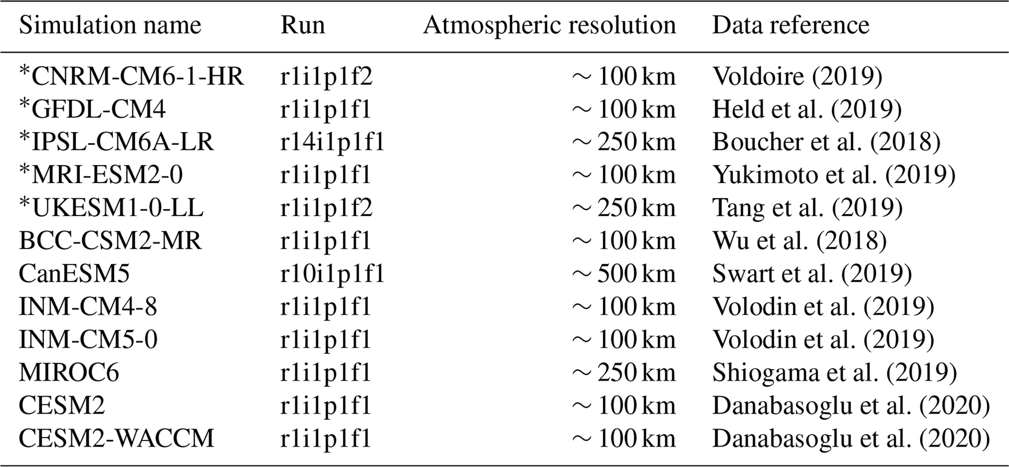
The same variables (T and PR) are also extracted for the period 1981–2100 from 12 global climate models (GCMs) contributing to the sixth exercise of the Coupled Model Intercomparison Project (CMIP6, Eyring et al., 2016). This selection was dictated by the availability of T and PR fields at a daily timescale at the time of analysis: we have only selected models whose data were fully available for the whole period of 1981–2100. The list of GCMs used is provided in Table 1.

Voldoire (2019)Held et al. (2019)Boucher et al. (2018)Yukimoto et al. (2019)Tang et al. (2019)Wu et al. (2018)Swart et al. (2019)Volodin et al. (2019)Volodin et al. (2019)Shiogama et al. (2019)Danabasoglu et al. (2020)Danabasoglu et al. (2020)

Table 1 List of CMIP6 simulations used in this study, along with their run, approximate horizontal atmospheric resolution, and references. The models preceded by a “*” are the five models used in the ERA5 experiment (Sects. 4.1 and 5.1) and the perfect model experiment (Sects. 4.2 and 5.2). All 12 models are used in the sensitivity experiment (Sects. 4.3 and 5.3). See text for details.

To ease the handling of the different simulated and reference datasets, all temperature and precipitation fields have been regridded to a common spatial resolution of 1°×1°. Moreover, for the sake of simplicity, in the following, we only consider winter defined as December–January–February (DJF) and summer data (June–July–August, JJA) separately to investigate and test our α-pooling approach. Then, for each grid point and each dataset, the univariate CDFs of temperature and precipitation are calculated. Here, empirical distributions are employed (i.e. step functions via the “ecdf” R function) in order not to fix the distribution family and thus let the data “speak for themselves”. Other parametric or nonparametric CDF modelling methods can be used if needed and appropriate.

3 Combining models via the CDF-pooling approach

The CDF of a random variable X is the function $F:\mathbb{R}\to [\mathrm{0},\mathrm{1}]$ defined as the probability that X is less than or equal to x, i.e. $F\left(x\right)=P(X\le x)$. Combining CDFs thus essentially amounts to combining, or aggregating, probabilities for all values x in a way that makes the aggregated function a CDF, i.e. a non-decreasing function with ${lim}_{x\to -\mathrm{\infty }}F\left(x\right)=\mathrm{0}$ and ${lim}_{x\to \mathrm{\infty }}F\left(x\right)=\mathrm{1}$.

Allard et al. (2012) offer a review of probability aggregation methods in geoscience, with application in spatial statistics. Aggregation or pooling methods can be characterized according to their mathematical properties. Let us denote $p_{\mathrm{1}},\mathrm{\dots },p_N$ as the probabilities to be pooled together and p_G as the resulting pooled probability. A pooling method verifying p_G=p when p_i=p for all $i=\mathrm{1},\mathrm{\dots },N$ is said to preserve unanimity. Furthermore, let us suppose that we are in the following case: at least one index i exists such that p_i=0 (p_i=1) with $\mathrm{0}<p_j<\mathrm{1}$ for j≠i. A pooling method which returns p_G=0 (p_G=1) in this case is said to enforce a certainty effect, a property also called the 0/1 forcing property. Notice that for a pooling method verifying this property, deadlock situations are possible when p_i=0 and p_j=1 for j≠i.

In the following, we will consider that there are N CDFs F_i(x), with $i=\mathrm{1},\mathrm{\dots },N$. Pooling methods must be applied simultaneously to all probabilities $P(X\le x)=F\left(x\right)$ and $P(X>x)=\mathrm{1}-F\left(x\right)$. The aggregated (or pooled) CDF must verify all properties of a proper CDF recalled above.

3.1 Pre-processing: standardizing data

CDFs from climate model simulations can be very different from each other and from ERA5 CDFs. It is thus necessary to perform a preliminary standardization (i.e. basic adjustment) before pooling them. Note that the same operation is performed in many IPCC figures (IPCC WGI, 2021) when working on anomalies (instead of raw simulated or reference data). This allows easier comparison (and combination) of the different datasets. In the present study, temperature and precipitation are standardized differently. For temperature, the simulated data are rescaled such that the mean and standard deviation correspond to those of the reference data:

$$\begin{array}{}\text{(1)}& T_{\text{rescaled}}={\displaystyle \frac{T-m_{\text{mod}}}{{\mathit{\sigma }}_{\text{mod}}}}\times {\mathit{\sigma }}_{\text{ref}}+m_{\text{ref}},\end{array}$$

where m_mod and σ_mod are the mean and standard deviation of the model data to rescale, and m_ref and σ_ref are those from ERA5. For precipitation, the data are rescaled to get the 90 % quantile similar to that of the reference precipitation:

$$\begin{array}{}\text{(2)}& {\text{PR}}_{\text{rescaled}}=\text{PR}\times {\text{Q90}}_{\text{ref}}/{\text{Q90}}_{\text{mod}},\end{array}$$

where Q90_ref and Q90_mod are respectively the 90 % quantiles from ERA5 and the model data to rescale. This choice of 90 % is a trade-off that enables having a robust quantile estimation and also a sufficient spread in the range of precipitation values (Vrac et al., 2016).

In the rest of this paper, all tested pooling methods are then applied to standardized data. As a preliminary step to our new α-pooling approach, we first briefly present the linear pooling and log-linear pooling with their main properties.

3.2 Linear pooling

The linear pooling, whose resulting pooled CDF is denoted as F_L, is simply a weighted average of all CDFs:

$$\begin{array}{}\text{(3)}& F_{\mathrm{L}}\left(x\right)=\sum _{i=\mathrm{1}}^N{w}_i{F}_i\left(x\right),\forall x\in \mathbb{R}.\end{array}$$

F_L is a proper CDF if and only if all w_i values are non-negative and ${\sum }_{i=\mathrm{1}}^N{w}_i=\mathrm{1}$. Note that with linear pooling, the probabilities are weighted for a given value x, which is quite different than averaging the quantiles for a given probability, as done in a usual weighted MMM (e.g. Markiewicz et al., 2020). Indeed, in our linear pooling (Eq. 3), the weighted average is performed on the CDFs (i.e. probabilities F_i(x)) and not on quantiles (values) of the variable. While there is not an inherent problem with linear pooling, like any linear approach, the method may lack flexibility and thus fail to capture the necessary non-linearity required to adjust to the data and their CDF. That is why non-linear methods (e.g. log-linear pooling) have been developed.

3.3 Log-linear pooling

The log-linear pooled CDF, denoted as F_LL, is found by considering that its logarithm is, up to a normalizing factor, a weighted average of the logarithm of the CDFs. Applying this to F(x) and 1−F(x) simultaneously, one gets

$$\begin{array}{c}{\displaystyle }\ln F_{\text{LL}}\left(x\right)=K+\sum _{i=\mathrm{1}}^N{w}_i\ln F_i\left(x\right)\mathrm{\text{and}}\\ {\displaystyle }\ln (\mathrm{1}-F_{\text{LL}}(x\left)\right)=K+\sum _{i=\mathrm{1}}^N{w}_i\ln (\mathrm{1}-F_i(x\left)\right),\end{array}$$

where $w_{\mathrm{1}},\mathrm{\dots },w_N$ is a set of N non-negative weights and K is the normalizing factor. After some algebra, one finally obtains

$$\begin{array}{}\text{(4)}& F_{\text{LL}}\left(x\right)={\displaystyle \frac{{\prod }_{i=\mathrm{1}}^N{F}_i(x{)}^{w_i}}{{\prod }_{i=\mathrm{1}}^N{F}_i(x{)}^{w_i}+{\prod }_{i=\mathrm{1}}^N(\mathrm{1}-F_i\left(x\right){)}^{w_i}}},\forall x\in \mathbb{R},\end{array}$$

which is a proper CDF for all non-negative weights w_i. The condition $S={\sum }_{i=\mathrm{1}}^N{w}_i=\mathrm{1}$ entails unanimity. In simulations, Allard et al. (2012) showed that log-linear pooling of probabilities consistently leads to the best validation scores among all other tested pooling methods. However, log-linear pooling verifies the 0/1 forcing property. This is not necessarily a desirable property since F_LL belongs to the interval (0,1) only for the restricted set of values x such that $\mathrm{0}<F_i\left(x\right)<\mathrm{1}$ for all $i=\mathrm{1},\mathrm{\dots },N$. Moreover, F_LL is undefined as soon as a pair i,j exists with i≠j such that F_i(x)=0 and F_j(x)=1.

3.4 α Pooling

In order to mitigate the problems faced with the log-linear pooling and the lack of flexibility of the linear pooling, we propose α pooling. Its theoretical expression is presented here. How the parameters are estimated from the models and the reference is shown in the next section. Our approach builds on the A_α-IT transformation proposed in Clarotto et al. (2022), which uses the less stringent power transformation instead of the log transformation used in the log-linear pooling approach. We first recall briefly that a D-part composition is a vector $(v_{\mathrm{1}},\mathrm{\dots },v_D{)}^t$ of D non-negative values such that ${\sum }_{i=\mathrm{1}}^D{v}_i=\mathit{\kappa }$, where κ is an arbitrary positive constant which can be set equal to 1 without loss of generality. In all generality, A_α-IT transforms a composition with D parts (constrained to belong to the simplex of dimension D−1) to a vector with D−1 unconstrained and well-defined coordinates, even when some parts are equal to 0 (Clarotto et al., 2022). For all x∈ℝ, the vector $\mathit{F}\left(x\right)=\left(F\right(x),\mathrm{1}-F(x){)}^t$ can be seen as a two-part composition. In this case, the A_α-IT transformation of F(x) results in a scalar:

$$\begin{array}{}\text{(5)}& z\left(x\right)=A_{\mathit{\alpha }\text{-IT}}\left(\mathit{F}\right(x\left)\right)={\mathit{\alpha }}^{-\mathrm{1}}{\mathit{H}}_{\mathrm{2}}\mathit{F}(x{)}^{\mathit{\alpha }},\end{array}$$

where H₂ is the (1,2) Helmert matrix $(\sqrt{\mathrm{2}},-\sqrt{\mathrm{2}})$ and where F(x)^α is the vector $\left(F\right(x{)}^{\mathit{\alpha }},(\mathrm{1}-F(x){)}^{\mathit{\alpha }}{)}^t$ with α>0. The α pooling postulates a linear aggregation of the scores z_i(x) with

$$\begin{array}{}\text{(6)}& {\displaystyle }\begin{array}{rl}{\displaystyle }{z}_G\left(x\right)& {\displaystyle }={\sum }_{i=\mathrm{1}}^N{w}_i{z}_i\left(x\right)\\ {\displaystyle }& {\displaystyle }={\displaystyle \frac{\sqrt{\mathrm{2}}}{\mathit{\alpha }}}{\sum }_{i=\mathrm{1}}^N{w}_i\left(F_i\right(x{)}^{\mathit{\alpha }}-(\mathrm{1}-F_i(x\left){)}^{\mathit{\alpha }}\right),\end{array}\end{array}$$

where, as above, $w_{\mathrm{1}},\mathrm{\dots },w_N$ is a set of N non-negative weights summing to 1, i.e. with ${\sum }_{i=\mathrm{1}}^N{w}_i=\mathrm{1}$. The α-pooling aggregated CDF F_G is thus the CDF such that $z_G\left(x\right)=\frac{\sqrt{\mathrm{2}}}{\mathit{\alpha }}\left(F_G\right(x{)}^{\mathit{\alpha }}-(\mathrm{1}-F_G(x\left){)}^{\mathit{\alpha }}\right)$. Hence, for each x, F_G(x) solves

$$\begin{array}{}\text{(7)}& {\displaystyle }\begin{array}{rl}{\displaystyle }{F}_G(x{)}^{\mathit{\alpha }}& {\displaystyle }-(\mathrm{1}-F_G(x){)}^{\mathit{\alpha }}=\mathit{\alpha }{z}_G(x)\\ {\displaystyle }& {\displaystyle }={\sum }_{i=\mathrm{1}}^N{w}_i\left(F_i\right(x{)}^{\mathit{\alpha }}-(\mathrm{1}-F_i(x\left){)}^{\mathit{\alpha }}\right).\end{array}\end{array}$$

Let us define the function

$$\begin{array}{}\text{(8)}& G\left(y\right)={\mathit{\alpha }}^{-\mathrm{1}}\left[y^{\mathit{\alpha }}-(\mathrm{1}-y{)}^{\mathit{\alpha }}\right],\end{array}$$

with $\mathrm{0}\le y\le \mathrm{1}$. G(y) is an increasing one-to-one function on [0,1], with $G\left(\mathrm{0}\right)=-{\mathit{\alpha }}^{-\mathrm{1}}$, $G(\mathrm{1}/\mathrm{2})=\mathrm{0}$ and $G\left(\mathrm{1}\right)={\mathit{\alpha }}^{-\mathrm{1}}$. One thus gets $F_G\left(x\right)=G^{-\mathrm{1}}\left(z_G\right(x\left)\right)$, where G⁻¹ is the inverse function of G, which exists and is unique. There is unfortunately no general closed-form solution to Eq. (7) for all values of α, but the aggregated probability can be found as

$$\begin{array}{}\text{(9)}& F_G\left(x\right)=G^{-\mathrm{1}}\left(z_G\right(x\left)\right)=\arg \underset{y\in [\mathrm{0},\mathrm{1}]}{min}{\left(G\left(y\right)-z_G\left(x\right)\right)}^{\mathrm{2}}\end{array}$$

using numerical optimization. It is straightforward to check that when α=1, the solution to Eq. (7) is the linear pooling. Likewise, using ${lim}_{\mathit{\alpha }\to \mathrm{0}}{F}_i(x{)}^{\mathit{\alpha }}=\mathrm{1}+\mathit{\alpha }\ln F_i(x)$, it is easy to check that the α pooling tends to the log-linear pooling as α→0. We can show the following.

Proposition 1. The function F_G(x) defined in Eqs. (7) and (9) is a proper CDF.

Proof. The derivative of z_G(x) with respect to x is $z_G(x{)}^{\prime }=\sqrt{\mathrm{2}}{\sum }_{i=\mathrm{1}}^N{w}_i{f}_i(x\left)\right(F_i(x{)}^{\mathit{\alpha }-\mathrm{1}}+(\mathrm{1}-F_i\left(x\right){)}^{\mathit{\alpha }-\mathrm{1}})\ge \mathrm{0}$. Hence, z_G(x) is a non decreasing function of x. Since the derivative of the function G(y) with respect to y is also positive, the function $F_G\left(x\right)=G^{-\mathrm{1}}\left(z_G\right(x\left)\right)$ is increasing because it is the composition of two increasing functions. In addition, using ${lim}_{x\to -\mathrm{\infty }}{F}_i\left(x\right)=\mathrm{0}$ and ${lim}_{x\to \mathrm{\infty }}{F}_i\left(x\right)=\mathrm{1}$ together with ${\sum }_{i=\mathrm{1}}^N{w}_i=\mathrm{1}$, it is easy to check that ${lim}_{x\to -\mathrm{\infty }}{F}_G\left(x\right)=\mathrm{0}$ and ${lim}_{x\to \mathrm{\infty }}{F}_i\left(x\right)=\mathrm{1}$. Hence, F_G is a proper CDF. □

The α pooling presented in Eq. (7) mitigates the principal inconvenience of the log-linear pooling, since it eliminates the 0/1 forcing property and it is well defined for all values of F_i(x). In addition it seamlessly accommodates the case F_i(x)=0 and F_j(x)=1 with i≠j.

Remark 1. The constraint on the sum of the weights can be relaxed. In this case, if $S={\sum }_{i=\mathrm{1}}^N{w}_i>\mathrm{1}$, F_G will still be a proper CDF because y is constrained to belong to the interval [0,1] in Eq. (9). But if S<1, the lower and upper limits of F_G will not be equal to 0 and 1, respectively, with ${lim}_{x\to -\mathrm{\infty }}{F}_G\left(x\right)=G^{-\mathrm{1}}(-S/\mathit{\alpha })=b>\mathrm{0}$ and ${lim}_{x\to \mathrm{\infty }}{F}_G\left(x\right)=G^{-\mathrm{1}}(S/\mathit{\alpha })=\mathrm{1}-b<\mathrm{1}$.

In Appendix A, we present a closed-form expression which is a very good approximate solution to Eq. (7) in most cases, i.e. except when S>1. Then in Appendix B, we present some optimal properties of the α pooling presented above related to the fact that α pooling derives from the general class of quasi-arithmetic pooling methods and corresponds to a proper scoring rule (Neyman and Roughgarden, 2023).

An illustration is provided in Fig. 1a for N=3 distributions F₁, F₂, and F₃ to be combined, respectively corresponding to a lognormal CDF, a Gaussian one, and a Student's t distribution. A uniform CDF is arbitrarily fixed as a reference. Despite the fact that they belong to very different families, the four CDFs are constructed here such that they have the same mean and variance; i.e. they respect the constraints of our real-case application (see Sect. 3.1). For this example, the estimated α parameter tends to 0 and w₁=0.06, w₂=0.79, and w₃=0. The higher value for w₂ than for w₁ or w₃ indicates that the reference uniform CDF is closer to F₂ (i.e. the Gaussian distribution) than to the others, which was expected considering the behaviour of F₁ and F₃ in the lower tail. Overall, given the difficulty of the illustration (very different CDFs), the α-pooling pooled CDF (shown by the dashed black line in Fig. 1a) is able to approximate the reference CDF reasonably well (blue line), despite some larger errors on the upper tail. Notice that it performs significantly better than the linear pooling (red and green lines). In addition, Fig. 1b displays the z scores (i.e. G as a function of x in Eq. 8) for the three CDFs to be combined, the reference one and the resulting α-pooling CDF.

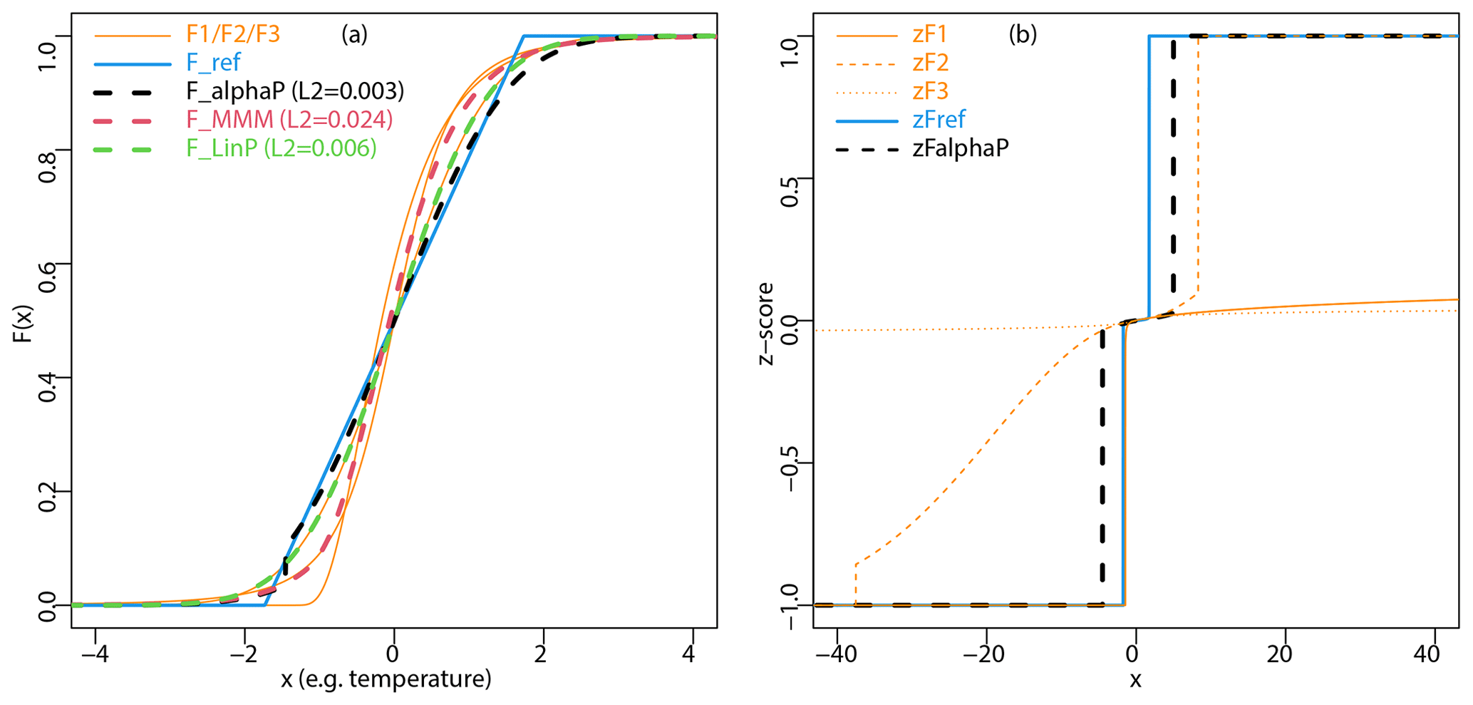
Figure 1 Illustration for N=3 distributions F₁, F₂, and F₃ to be combined, respectively corresponding to a lognormal CDF, a Gaussian one, and a Student's t distribution. A uniform CDF is arbitrarily fixed as a reference. Note that the four CDFs are constructed here with the same mean and variance to respect the constraints of our real-case application. Panel (a) displays the three CDFs to combine (orange lines), the reference CDF (blue line), and the resulting α-pooling CDF (dashed black line), MMM CDF (dashed red line), and linear pooling CDF (dashed green line). For each pooling method, the value of the L² norm between the resulting CDF and the reference one (i.e. the quadratic distance Q in Eq. 10) is also indicated. Note that the reference is not used to perform MMM. Panel (b) shows the z scores (i.e. function G in Eq. 8, where z=G(F(x)) with F(x) the CDF) for the three CDFs to be combined, the reference one, and the α-pooling CDF.

3.5 Estimating the parameters and computing the aggregated CDF

Given N CDFs F_i, $i=\mathrm{1},\mathrm{\dots },N$ and a reference CDF F₀, the parameters are estimated by minimizing the quadratic distance:

$$\begin{array}{}\text{(10)}& Q=\sum _{k=\mathrm{1}}^K(x_k-x_{k-\mathrm{1}})\left(F_{\mathrm{0}}\right(x_k)-F_G(x_k){)}^{\mathrm{2}},\end{array}$$

where F_G(x) is obtained by solving Eq. (7) and where $x_{\mathrm{0}},\mathrm{\dots },x_K$ is an increasing sequence discretizing the real line. The L-BFGS-B optimization algorithm (Byrd et al., 1995) is launched to minimize Eq. (10) and find the weights and the α parameter. This algorithm is a limited-memory extension of the BFGS quasi-Newton method and allows handling simple bound constraints on the variables. The parameter α and the weights must be positive, and the weights can be constrained to sum to 1 or not. In the following, the sum S of weights is let free, i.e. not necessarily equal to 1. Indeed, preliminary results indicated that this freedom gives more flexibility to the α pooling and thus better aggregated CDFs (not shown). When unconstrained, it was found that in most cases the optimal sum S was close to 1. There are two reasons for this: when S<1, the pooled CDF varies from b to 1−b (see Remark 1). As a consequence, b must be as close to 0 as possible and hence S as close to 1 as possible for the pooled CDF to be close to the reference; when S>1, the inverse of all values $z_G<-\mathrm{1}/\mathit{\alpha }$ (values $z_G>\mathrm{1}/\mathit{\alpha }$) leads to the same inverse equal to 0 (1). A value of S that is too high is therefore likely to lead to a lack of fit in the lower and upper tails. However, when S<1, as the aggregated CDF goes from b>0 to $\mathrm{1}-b<\mathrm{1}$, it is not a proper CDF per se. Hence, a “min–max” rescaling of the aggregated CDF F_G is performed such that the rescaled CDF F_resc is always in [0,1].

$$\begin{array}{}\text{(11)}& {\displaystyle }\begin{array}{rl}{\displaystyle }{F}_{\text{resc}}\left(x\right)& {\displaystyle }={\displaystyle \frac{F_G\left(x\right)-{min}_x\left(F_G\right(x\left)\right)}{{max}_x\left(F_G\right(x\left)\right)-{min}_x\left(F_G\right(x\left)\right)}}\\ {\displaystyle }& {\displaystyle }={\displaystyle \frac{F_G\left(x\right)-b}{(\mathrm{1}-b)-b}}={\displaystyle \frac{F_G\left(x\right)-b}{\mathrm{1}-\mathrm{2}b}}\end{array}\end{array}$$

In practice, this rescaling is only very slight as b is very often found to be extremely small, say less than 10⁻³.

The weights are easily interpretable since, as a rule, the higher the weight w_i, the closer F_i is to the reference F₀. The parameter α has a less immediate interpretation. As shown in Clarotto et al. (2022), the A_α-IT transform can be seen as a difference between the Box–Cox transformation of F(x) and that of (1−F(x)) (see also Appendix A). The parameter α can thus be interpreted as the power necessary to deform all CDFs (reference and models) in order to get an optimal linear pooling for these deformed CDFs, from log transform (α→0) to no transform (α=1), to quadratic transform (α=2).

3.6 Benchmarking α pooling: CDF multi-model mean (MMM) and linear pooling

As a benchmark for evaluating the α-pooling approach, two CDF pooling methods are also applied. The first one is the simplest and consists of defining a “mean” CDF based on the N CDFs to be combined. Let us consider, for example, N=2 GCMs with CDFs F₁ and F₂, say of temperature, for a given grid cell. For any temperature value x, the mean CDF F_MMM(x) corresponds to the average of F₁(x) and F₂(x). An example is given in Fig. 1a for the three distributions used to illustrate the α-pooling method. Here, F_MMM is shown as a dashed red line. Note that, for MMM, the reference CDF is not used at all, as the N CDFs are linearly averaged with weights all equal to $\mathrm{1}/N$, whatever the quality of the different model CDFs with respect to that of the reanalysis. Hence, it is not surprising that α pooling better approximates the reference CDF over the calibration period.

The second CDF pooling method applied for comparison is the linear pooling described in Eq. (3). Here, contrary to MMM, the reference CDF is used to infer the weight parameters. By comparing the linear and α-pooling methods, we can assess the potential added value brought by the alpha parameter.

The same illustration as previously used is also given in Fig. 1a for linear pooling, with the dashed green line. Based on this illustrative – but difficult – example, it is clear that the introduction of the α parameter allows us to get closer to the reference CDF, at least over the calibration period. This is clear from the value of the L² norm computed between the resulting CDF (i.e. α pooling, linear pooling, or MMM) and the reference: α pooling has the smallest L² (0.003), and linear pooling's L² is doubled (0.006), while it is almost 10-fold for MMM (0.024). However, one major objective of this study is also to evaluate how MMM, linear pooling, and α pooling behave in a projection period wherein climate changes occurs. When driven only by model CDFs over a projection (future) period, are the three pooling methods able to capture the changes in reference (temperature or precipitation) CDFs?

3.7 Bias corrections from CDF pooling results

The aggregated CDF can be used within a CDF-based bias correction method applied to GCMs and, hence, to obtain corrected simulations in a way that preserves the temporal rank dynamics. Indeed, once $\widehat{F}$ is estimated over a projection period, one can apply a quantile mapping technique (e.g. Gudmundsson et al., 2012, among many others) between $\widehat{F}$ and the CDF F_m of a given model m over the same period: for any value x simulated by model m, it consists of finding the value y such that $\widehat{F}\left(y\right)=F_m\left(x\right)$ which is equivalent to

$$\begin{array}{}\text{(12)}& y={\widehat{F}}^{-\mathrm{1}}\left(F_m\right(x\left)\right),\end{array}$$

where ${\widehat{F}}^{-\mathrm{1}}$ is the inverse CDF, allowing computing the quantile associated with a given probability. Therefore, by applying Eq. (12) successively to all simulations from model m, we can obtain bias corrections. Those have the same rank chronology as that of model m but their values follow distribution $\widehat{F}$. By applying this bias correction technique to the different models employed within the MMM, linear pooling, or α-pooling methods, the N bias-corrected time series have the exact same distribution (i.e. $\widehat{F}$) but their temporal dynamics are different, as stemming from the N models.

3.8 Model-by-model bias correction via CDF-t

To evaluate the pros and cons of the bias corrections brought by the proposed pooling approaches, a more traditional “model-by-model” bias correction method is also applied for comparison: the “cumulative distribution function – transform” (CDF-t) method (Michelangeli et al., 2009; Vrac et al., 2012). It consists of a quantile mapping technique (e.g. Panofsky and Brier, 1968; Haddad and Rosenfeld, 1997; Déqué, 2007; Gudmundsson et al., 2012) allowing accounting for changes in the distributional properties of the climate simulations from the reference to the projection period. The reference CDF F_Rp over the projection period is first estimated as a composition of F_Rc, F_Mc, and F_Mp, as well as the reference CDF over the calibration period, the model CDF over the calibration period, and the projection period:

$$\begin{array}{}\text{(13)}& {\widehat{F}}_{\text{Rp}}\left(x\right)=F_{\text{Rc}}\left(F_{\text{Mc}}^{-\mathrm{1}}\right(F_{\text{Mp}}\left(x\right)\left)\right),\end{array}$$

where $F_{\text{Mc}}^{-\mathrm{1}}$ is the inverse CDF of F_Mc. See Vrac et al. (2012) or François et al. (2020) for more details. Based on the estimated projection reference CDF, a quantile mapping is then fitted between ${\widehat{F}}_{\text{Rp}}$ and F_Mp to bias-correct the simulations from the model M. Hence, in the case of N climate models to adjust, N CDF-t bias corrections are defined and applied.

4 Design of experiments

In the following, three experiments are described to evaluate and compare α pooling, linear pooling, MMM, and CDF-t. For the sake of clarity and space, these experiments are carried out separately over two seasons only: winter (December, January, February – DJF) and summer (June, July, August – JJA). Only winter results are given in the following but summer results can be found in the Supplement.

4.1 ERA5 experiment

The first experiment considers ERA5 reanalysis as a reference. When considering linear and α-pooling methods, for each grid point and variable, we calibrate the approaches using N climate models with ERA5 data as a reference over the calibration period of 1981–2000. Then, we use the calibrated parameters (w_i and α) to combine the models CDFs over the projection period of 2001–2020. For CDF-t, the same calibration period (1981–2000) is used, and the corrections are made for each model independently for the projection period (2001–2020). For MMM, the CDFs of the climate models are directly averaged over 2001–2020. The results of each approach are then compared to the ERA5 data over 2001–2020.

In this experiment, only five GCMs are used. This is partly constrained by the α-pooling method that can have stability issues inferring the parameters when combining a large number of models. When a relatively high number of models (i.e. CDFs) are combined, such as 10, depending on the initialization values of the parameters in the inference algorithm, the “optimal” final parameters may vary. In essence, the optimized parameters are unstable in such a case. This is because many local minima attain undistinguishable L² distances. Indeed, while final parameters may differ between initializations, the minimized criterion values – specifically the quadratic distance in the CDF space outlined in Eq. (10) – remain relatively consistent, often converging to similar or nearly identical values. Although it has been tested with more than 10 models, the use of five GCMs appeared to be a good compromise in the sense that (i) it ensured not only stability in the quadratic criterion but also consistency in the final optimized parameters, (ii) it allows a reasonable computation time (e.g. no more than a few minutes of computations for each location and/or variable), and (iii) it employs a sufficient number of simulations to get robust results. These five GCMs (indicated with “*” in Table 1) were selected on the basis of a preliminary analysis showing that they approximately represent the spread of the future evolution of all 12 GCMs (not shown). Note that four models (IPSL-CM6A-LR, MRI-ESM2-0, UKESM1-0-LL, GFDL-CM4) out of the five selected ones are consistent with the choice made in the ISIMIP3 project (Lange and Büchner, 2021; Lange, 2021) for bias correction objectives.

The evaluations are performed in terms of biases of the obtained 2001–2020 temperature and precipitation with respect to ERA5. For each grid point, dataset, variable, and season (winter or summer), some statistics T are calculated. For temperature, statistics include the mean, standard deviation, and 99 % quantile (Q99). For precipitation, we consider the conditional mean given a wet state (Cm), probability of a dry day (P₁), and the 99 % quantile. A day with a PR value lower than 1 mm is considered dry (and thus > 1 mm wet).

Then, absolute biases are calculated as

$$\begin{array}{}\text{(14)}& B(m,T)=T\left(m\right)-T\left(\text{ERA5}\right)\end{array}$$

for temperature mean and Q99, while relative biases are calculated as

$$\begin{array}{}\text{(15)}& B(m,T)={\displaystyle \frac{T\left(m\right)-T\left(\text{ERA5}\right)}{T\left(\text{ERA5}\right)}}\end{array}$$

for temperature standard deviation and precipitation conditional mean, P₁, and Q99. m denotes the method (α pooling, linear pooling, MMM, or CDF-t) and T(X) the statistics calculated from dataset X (ERA5 or method results).

4.2 Perfect model experiment (PME)

As the ERA5 experiment evaluates the methods for a projection period (2001–2020) very close to the calibration one (1981–2000), it does not allow understanding their quality in a strong climate change context. To perform such an assessment, we propose a “perfect model experiment” (e.g. de Elía et al., 2002; Vrac et al., 2007, 2022; Krinner and Flanner, 2018; Robin and Vrac, 2021; Thao et al., 2022, among many others). The main idea is that one model, among N, is taken as the reference. For the four methods, the procedure is the following.

• α Pooling and linear pooling are calibrated to combine the other N−1 models over 1981–2000. The obtained parameters (i.e. w_i and α for α pooling or w_i only for linear pooling) are next used to combine the N−1 models over five different future 20-year periods: 2001–2020, 2021–2040, 2041–2060, 2061–2080, and 2081–2100.

• The same approach is followed for CDF-t: one model serves as a reference over 1981–2000 to calibrate CDF-t – here separately for each of the N−1 remaining models – which is then used to bias-correct each model simulation over the five future periods.

• As previously for the ERA5 experiment, MMM does not require any calibration. CDF averaging is directly applied to combine the N−1 models for each of the five periods.

Over each future period and each grid point, biases can then be evaluated with respect to the reference model. For temperature, it includes absolute biases (Eq. 14) of the mean, 1 % quantile, 99 % quantile, minimum, and maximum, as well as relative biases (Eq. 15) of standard deviation. For precipitation, relative biases are computed for the conditional mean a given wet state, probability of a dry (< 1 mm) day, standard deviation, conditional 99 % quantile a given wet state, unconditional 99 % quantile, and maximum.

Hence, no observational or reanalysis data are used as a reference in this experiment. Indeed, this PME is made under the “models are statistically indistinguishable from the truth” paradigm (e.g. Ribes et al., 2017), where “the truth and the models are supposed to be generated from the same underlying probability distribution” (Thao et al., 2022). Therefore, an evaluation framework based on this paradigm can consider any model as the reference. In practice in our PME, the same five models as in the ERA5 experiment (Sect. 4.1) are used and each model is used in turn as the reference. The four methods are thus tested on a diversity of possible references, encompassing cases where the truth can be either in the centre of the multi-model distribution or far in the tail.

4.3 Sensitivity of projected future CDFs to the choice of models

Finally, our third experiment aims to evaluate the uncertainty brought by the choice of the N models to combine and/or bias-correct. If this sensitivity is not very present over the calibration period – by construction, linear pooling, α pooling, and CDF-t are relatively close to the reference CDFs over this period – or over periods very close to the calibration, the results of the four methods applied to long-term future projections can be sensitive to the chosen N models. To evaluate this sensitivity, for each variable, linear pooling, α pooling, and CDF-t are calibrated with respect to ERA5 data over 1981–2000. Then, all methods are applied to 2081–2100 projections. However, in this experiment, linear pooling, α pooling, and MMM do not combine a unique set of five models (as in the ERA5 experiment). Instead, 100 different sets of N=5 models among the 12 presented in Table 1 are randomly drawn. The resulting 100 samples have been checked to contain each model in a uniform proportion (not shown). The linear pooling, α-pooling, and MMM methods are then applied 100 times, each with five models to combine, while CDF-t is applied to the 12 models separately. The 2081–2100 results obtained from each method and set of models do not allow any evaluation per se, as there is no reference over the future period. However, the use of multiple sets of models allows quantifying and comparing the statistical uncertainty brought by the choice of models for each method. In this experiment, for both temperature and precipitation, only six grid points are considered, corresponding to major capitals of the geographical domain: Paris (France), London (UK), Rome (Italy), Madrid (Spain), Berlin (Germany), and Stockholm (Sweden).

5 Results

5.1 ERA5 experiment results

Before looking at the results of the ERA5 experiment, it is interesting to visually understand how the α-pooling parameters are spatially distributed over the geographical domain. Hence, Fig. 2 displays maps of the winter (Fig. 2a and c) and summer (Fig. 2b and d) for the α parameter, temperature (Fig. 2a and b), and precipitation (Fig. 2c and d). First, note that the range of α is not the same for T and PR. While for temperature most of the values are lower than 1 (no unit), the range goes up to 2.5 for precipitation. Moreover, for both seasons, more pronounced spatial structures appear for T than for PR, with the latter α maps appearing more “pixelated”. This can be explained by the widely recognized spatial variability of precipitation, encompassing both occurrence and intensity, which is often challenging to accurately capture in climate models and thus reflected in the spatial diversity in the estimated alpha-pooling parameters. However, globally, even for PR, large regions share similar α values, indicating some spatial consistency of the parameters.

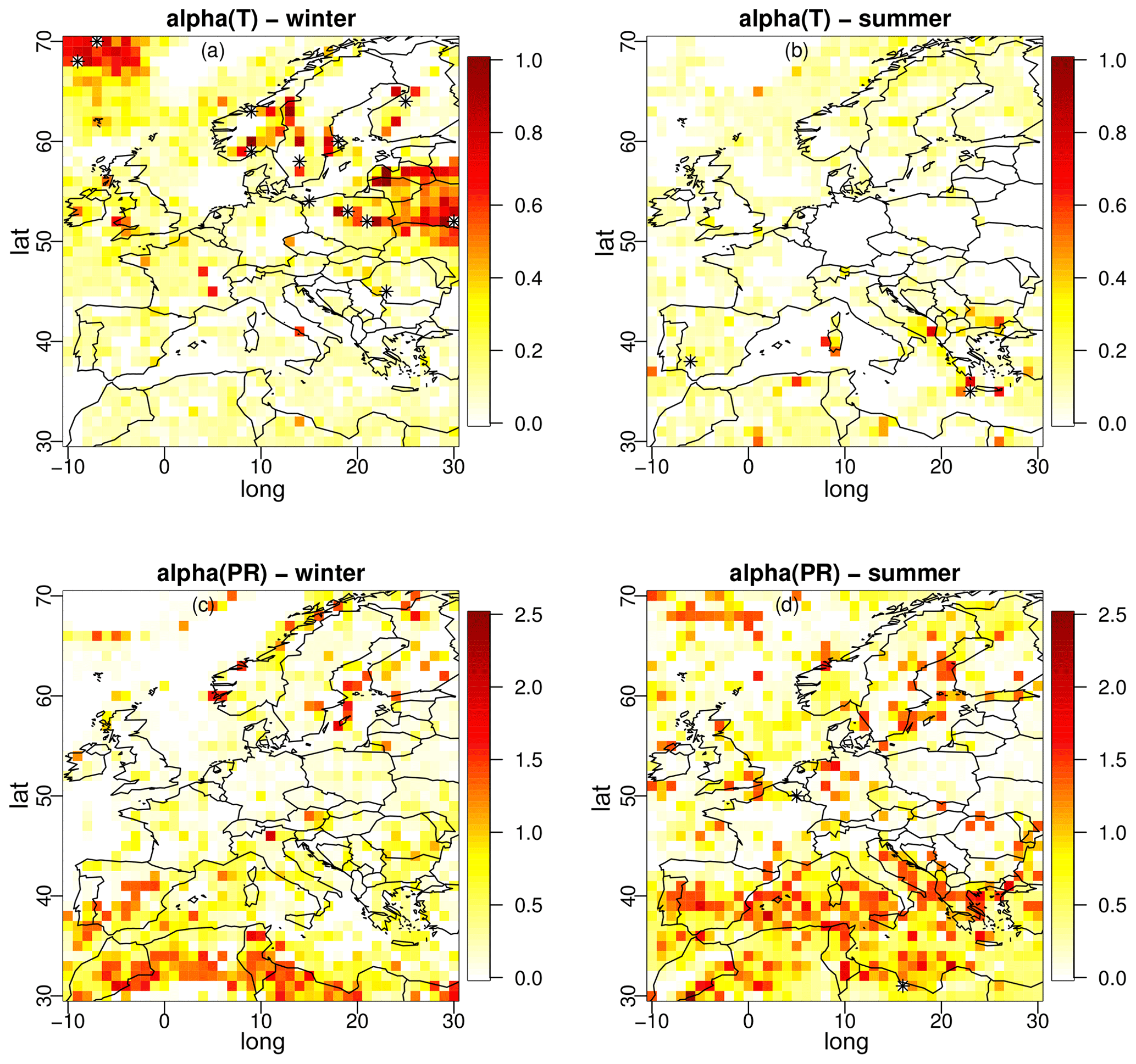
Figure 2 From α pooling, maps of the parameters α obtained within the ERA5 experiment for temperature (a, b) and precipitation (c, d) over winter (a, c) and summer (b, d) seasons.

Regarding the weight parameters of α pooling, winter maps are provided in Figs. 3 and 4 for temperature and precipitation, respectively. The results for summer are given in Figs. S1 and S2 in the Supplement. The spatial structures of the weights are clearly visible (for both T and PR) and even more pronounced than for the α maps. This strongly indicates that α pooling identifies large zones where some models have a larger influence on the combination and, thus, whose CDFs are closer to that of ERA5. Note, however, that for both variables, none of the models has the highest weights for all grid points of the domain. In other words, over this European region, each of the five models brings some valuable contribution, although there is contrast depending on the subregion. For example, with temperature, UKESM (Fig. 3e) shows the strongest contributions over the Mediterranean Sea, while MRI-ESM2 (Fig. 3d) displays the largest weights over the northeast part of the domain. Interestingly, the spatial distributions of the weights are not the same for T and PR. Thus, there is no clear link between the contribution of each variable, confirming that results from one variable cannot be generalized to another.

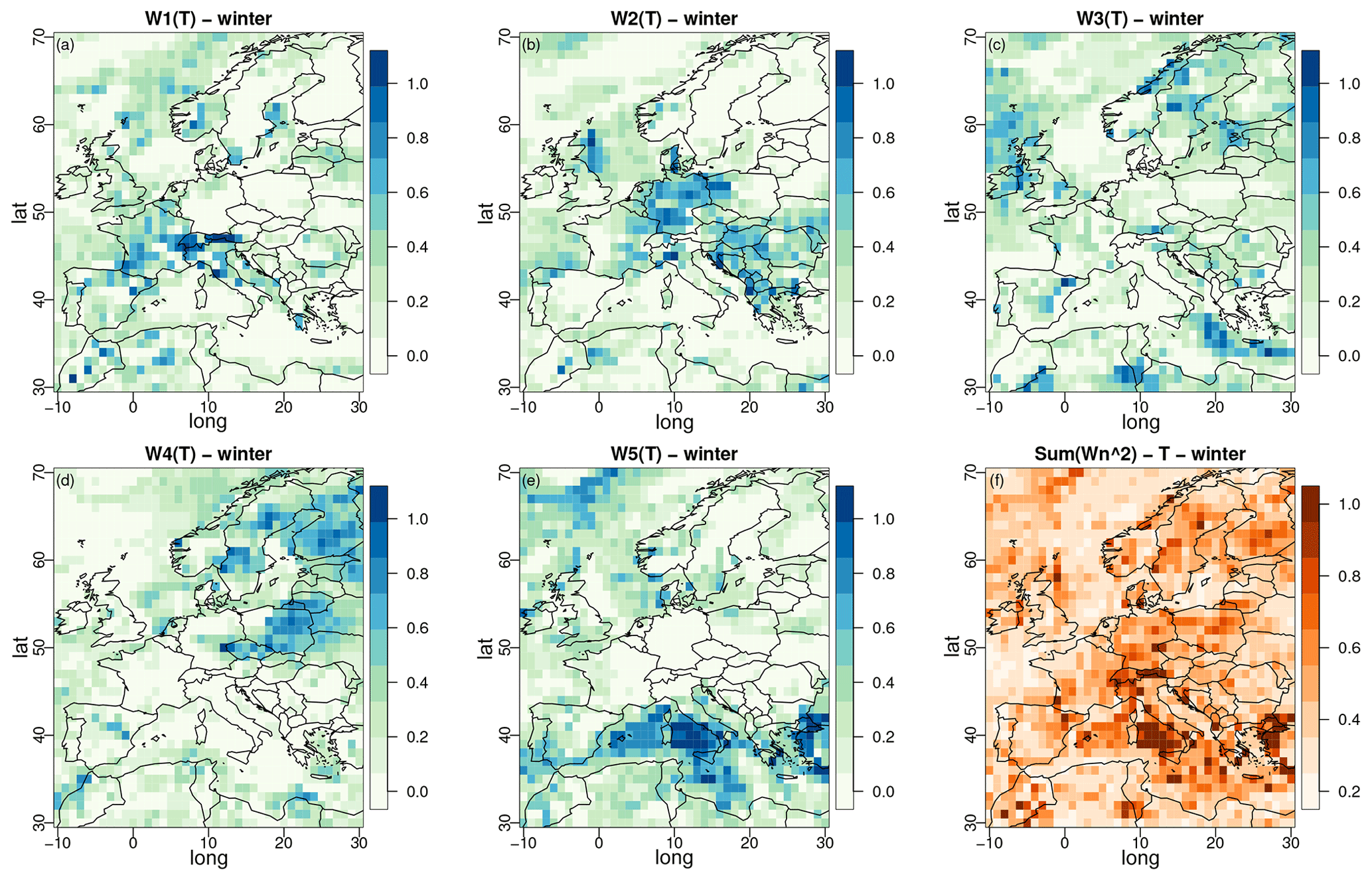
Figure 3 Maps of the weight parameters from α pooling for winter obtained with the ERA5 experiment for temperature over winter. Models 1 to 5 respectively correspond to CNRM-CM6-1-HR, GFDL-CM4, IPSL-CM6A-LR, MRI-ESM2-0, and UKESM1-0-LL. Panel (f) displays the concentration index, equal to sum of the squares of the five normalized weights. The results for summer are given in Fig. S1.

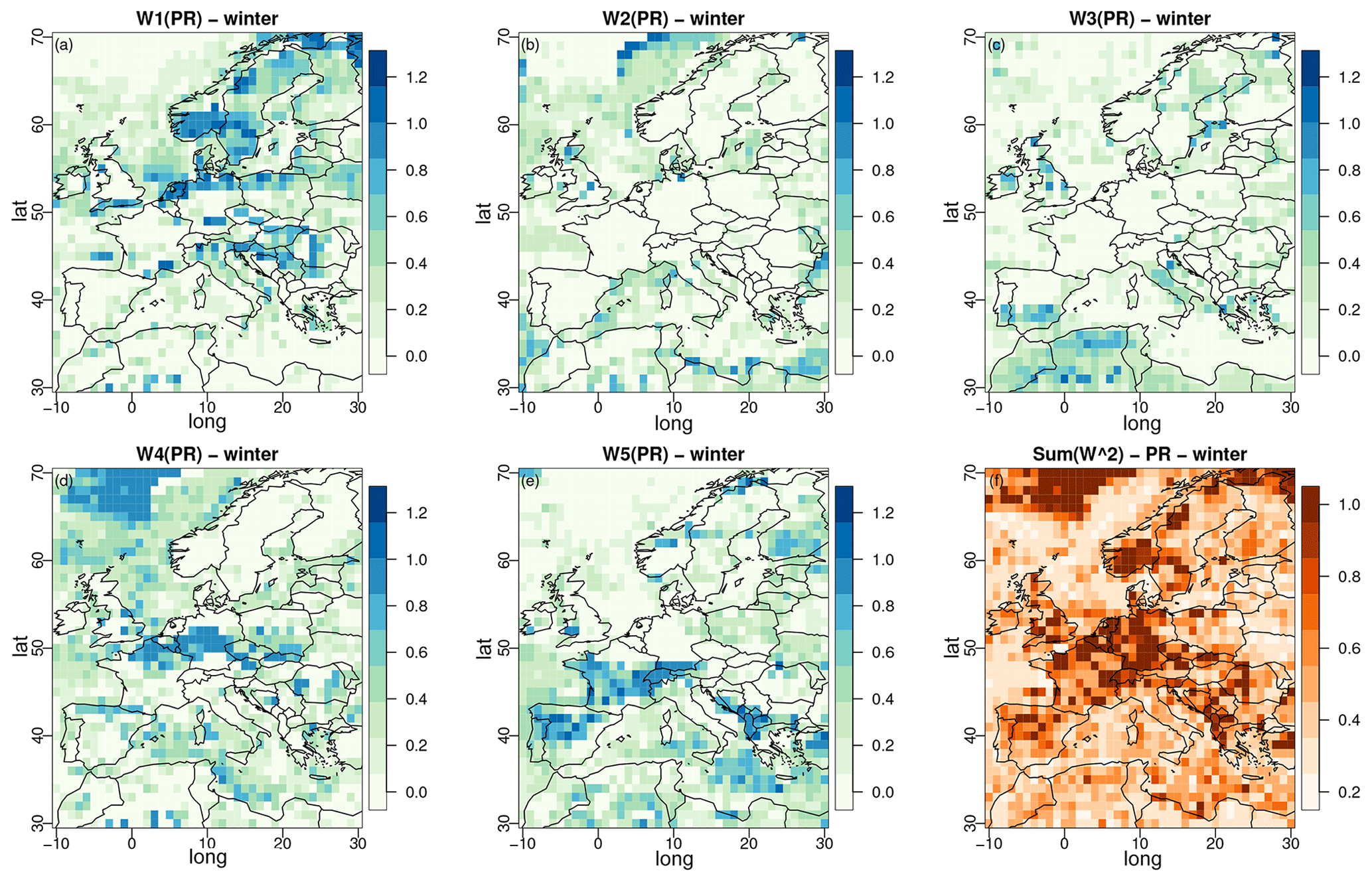
Figure 4 Same as Fig. 3 but for precipitation. The results for summer are given in Fig. S2.

A concentration index is displayed in panel (f) of Figs. 3 and 4, which is equal to the sum of the squares of the five normalized weights. It takes the value 1 when one single GCM takes all the weight and reaches a minimum of $\mathrm{1}/N=\mathrm{0.2}$ when the five normalized weights are equally distributed. The concentration index can only be applied to weights summing to 1. In our implementation of α pooling, the sum of weights is let free and, thus, not constrained to 1. Although this sum remains quite close to 1 (mostly between 0.95 and 1.05 for temperature and between 0.92 and 1.1 for precipitation, not shown), normalization is required, which is accomplished by dividing the weights by $S={\sum }_{i=\mathrm{1}}^N{w}_i$ before computing the concentration index. For temperature, Fig. 3f shows relatively well-distributed weights (most concentration indices between 0.2 and 0.7) despite two zones (close to Italy and close to Greece) strongly influenced by one single GCM (UKESM1, see Fig. 3e). For precipitation, more zones show a concentration index close to 1: for example, the northwestern part of the domain and northern France (MRI-ESM2, Fig. 4f), southern Norway and the northeastern part of the domain (CNRM-CM6, Fig. 4a), and the eastern Adriatic coast (UKESM1, Fig. 3e). Also note that the maps of weights obtained from linear pooling are given in Figs. S3 and S4 in the Supplement for temperature and Figs. S5 and S6 in the Supplement for precipitation. Interestingly, the spatial structures of the weights and concentration indices are very similar to those from α pooling. This confirms that the α parameter does not structurally modify the interpretation of the weights but brings additional flexibility.

The biases of the different methods with respect to 2001–2020 ERA5 are shown in terms of mean, standard deviation, and Q99 for winter temperature in Fig. 5 and in terms of conditional mean given a wet state, probability of a dry day (P₁), and Q99 for winter precipitation in Fig. 6. The equivalent figures for summer are provided in Figs. S7 and S8 in the Supplement for temperature and precipitation, respectively. In theses figures, the columns are associated with the different biases. The top row shows maps of biases for MMM: row 2 for α pooling, row 3 for CDF-t, and the fourth row for linear pooling. Note that, because CDF-t is applied separately for each GCM, the third row corresponds to the grid point median of the CDF-t biases. The fifth (bottom) row displays a more condensed view of the results via box plots of biases.

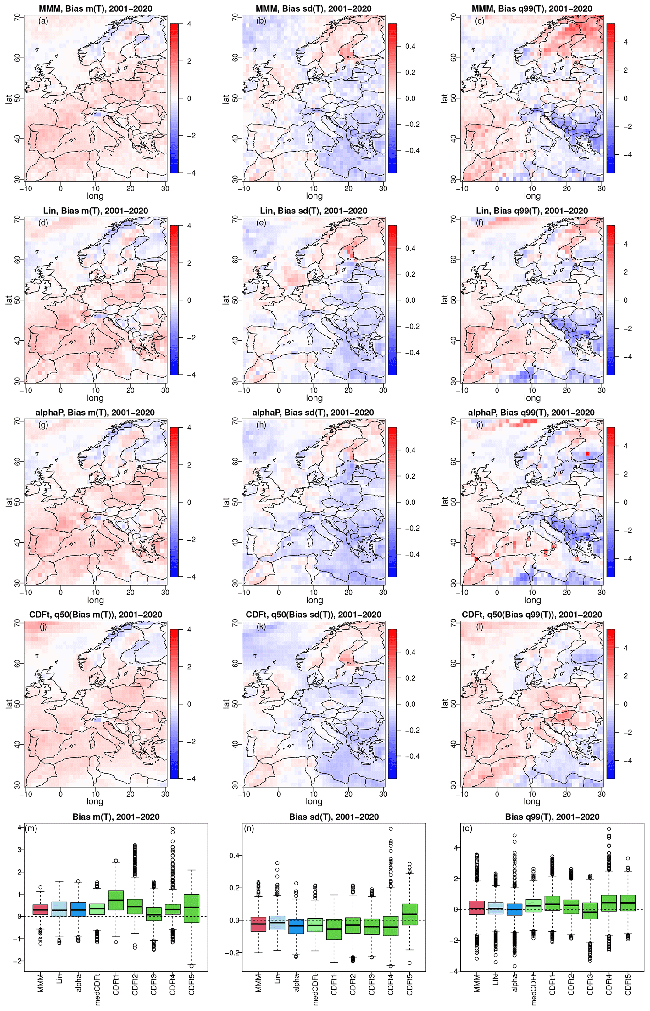
Figure 5 Biases in mean (left column: a, d, g, j, m), standard deviation (middle column: b, e, h, k, n), and 99 % quantile (right column: c, f, i, l, o) for winter temperature from MMM (a–c), α pooling (d–f), CDF-t (g–i), and linear pooling (j–l) under the 2001–2020 (projection) time period of the ERA5 experiment. Third row corresponds to the grid point median of the CDF-t biases. (m–o) Box plots of biases for MMM, linear pooling, α pooling, and the median CDF-t biases, as well as for each of the five CDF-t results. The results for summer temperature are given in Fig. S7.

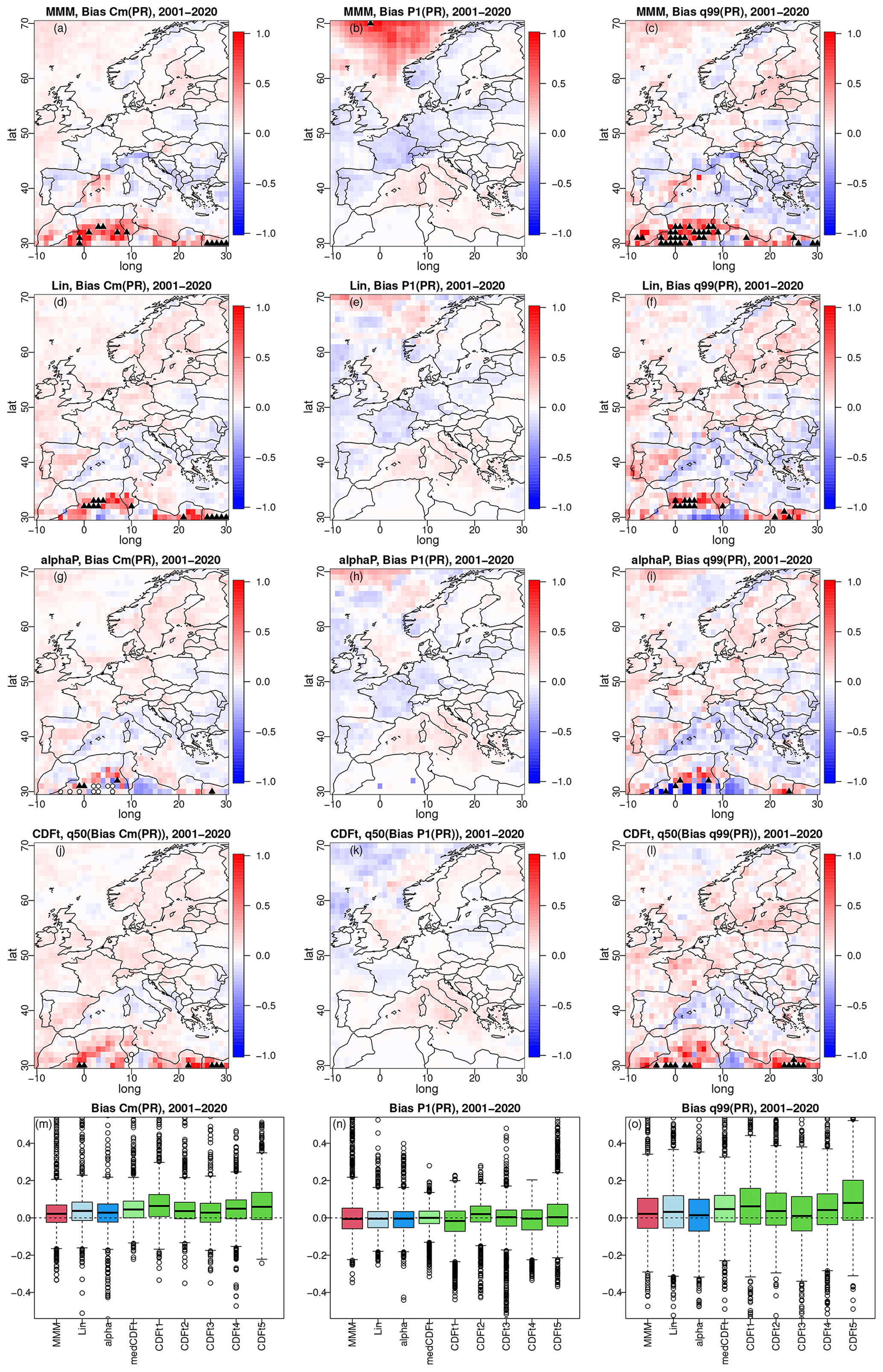
Figure 6 Same as Fig. 5 but for winter precipitation with biases in conditional mean given a wet state (left column: a, d, g, j, m), probability of a dry day (P₁, middle column: b, e, h, k, n), and 99 % quantile (right column: c, f, i, l, o). The results for summer are given in Fig. S8.

For temperature (Fig. 5), the differences between the maps of biases from the four methods are not very pronounced. This is especially true for the biases in mean temperature and standard deviation (SD). Some more differences appear for Q99. For instance, MMM (Fig. 5c) shows relatively high positive bias (∼ 4 °C) over the northeastern part of the domain (Sweden and Finland), while biases for α-pooling Q99 (Fig. 5f), CDF-t (median) (Fig. 5i), and linear pooling (Fig. 5l) do not present this structure. Also, the CDF-t median Q99 (Fig. 5i) has a positive (∼ 1–2 °C) bias pattern over the central domain (Germany, Italy, Poland, Hungary, Romania), while the three other methods show more nuanced and mixed structures. When looking at the more integrated box plot view (bottom row in Fig. 5), similar behaviour of α pooling, linear pooling, and MMM is visible for the three biases: the box plots are relatively equivalent from one method to another. However, even though this is also the case for the CDF-t median biases – at least for mean and SD and to some extent for Q99 – the individual CDF-t biases (i.e. GCM by GCM) show much larger variability, indicating that relying on a single GCM to perform the bias correction might lead to stronger errors within this ERA5 experiment.

For precipitation (Fig. 6), conclusions are somewhat similar, but some more differences between methods are now more visible. For example, in the Norwegian Sea, the relative biases of P₁ for MMM (Fig. 6b) have a large and strongly positive structure (∼ 1) that does not appear in the other methods. Another example is the mostly negative bias (∼ −1) in α-pooling Q99 (Fig. 6f) over the North African part of the domain, while MMM and (median) CDF-t show mostly highly positive biases and linear pooling more mixed patterns for this region. The box plot view for winter precipitation is similar to that for temperature: roughly equivalent box plots for the four methods, with more variability from the individual CDF-t results.

Note, however, that the ERA5 experiment results for summer (Figs. S7 and S8) show more differences between the four methods – especially in the box plots – slightly in favour of the linear pooling and α-pooling methods, which show box plots more centred around 0 for all biases and variables.

In the ERA5 experiment, the results are relatively similar for the four methods. This indicates that the added flexibility provided by α pooling may not be required over the 1981–2020 period of ERA5. This can nevertheless be different when considering other projection periods and reference datasets. Furthermore, the evaluation (2001–2020) and calibration (1981–2000) periods are quite close to each other, resulting in similar outcomes for both periods. These two results suggest that distinguishing between the different methods may be challenging in a climate that is relatively stable or undergoing minimal change. However, our primary objective is to assess and compare our various pooling strategies in the context of significant climate change. Given that climate changes (in temperature and precipitation) from 1980 to 2100 in the SSP8.5 CMIP6 simulations are significantly more pronounced than what can be seen in the whole ERA5 reanalysis dataset over western Europe, the perfect model experiment (PME) will effectively and more clearly fulfil this purpose.

5.2 PME results

PME is first applied here to winter temperature, and summer results are in the Supplement. For each period and method, the box plots of the different biases, computed at each grid point, are provided in Fig. 7 (PME summer temperatures are in Fig. S9 in the Supplement). As expected, for all biases, the more distant the period, the larger the box plots, indicating an increase in possible statistical errors for periods further in the future. For brevity, we now focus on the last period (i.e. p6, 2081–2100), which results in the most pronounced differences between methods. For mean T bias (Fig. 7a), all four approaches show similar performance, although CDF-t has a wider box plot. The bias of minimum temperature (Fig. 7e) is roughly equivalent for MMM and the linear or α-pooling approaches, while CDF-t presents, on average, a negative bias. However, α pooling appears slightly better than MMM and linear pooling for the temperature 1 % quantile (Q01, Fig. 7c), with CDF-t having a median bias (i.e. box plot centre) equivalent to α pooling but with larger variability. For maximum temperature (Fig. 7f), CDF-t shows a strongly positive bias, while its biases look reasonable – at least more comparable to the other methods – for standard deviation (Fig. 7b) and 99 % quantile (Q99, Fig. 7d). Globally, for temperature standard deviation (Fig. 7b), Q99 (Fig. 7d), and maximum value (Fig. 7f), α pooling is more robust than the other methods since it clearly provides smaller biases over the 2081–2100 period.

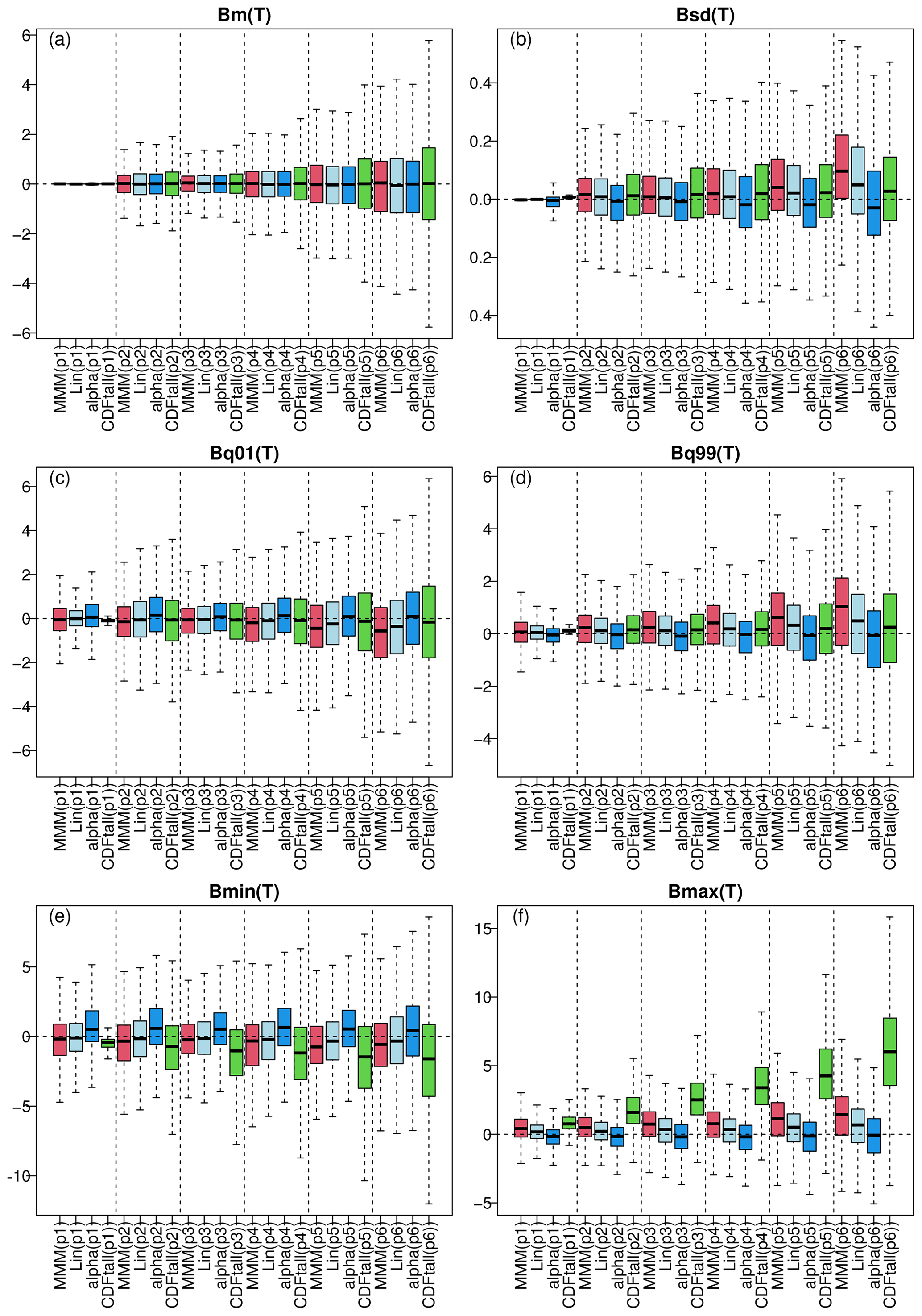
Figure 7 Results of the perfect model experiment for winter temperature: box plots of biases from the three methods (red: MMM, light blue: linear pooling, blue: α pooling, green: CDFt) for the six 20-year time periods (from p1 for 1981–2000 calibration to p6 for 2081–2100). The different panels display biases in (a) mean temperature, (b) standard deviation, (c) 1 % quantile, (d) 99 % quantile, and (e) minimum and (f) maximum temperature. Note that, for CDF-t, the box plots are drawn from the concatenation of all the individual CDF-t biases. Results for summer are provided in Fig. S9.

Figure 8 shows the PME results for winter precipitation (summer results are in Fig. S10 in the Supplement). As was the case for temperature, the more distant the period, the wider the box plots, although this is less pronounced here. Over 2081–2100, CDF-t results are often the most biased, except for the probability of a dry day (P₁, Fig. 8b) where it is as good as the other methods. As in Fig. 7f, the maximum values of precipitation from CDF-t (green box plot in Fig. 8f) show strong biases with a high variability. Regarding MMM, linear pooling, and α-pooling methods, they give roughly similar biases in terms of conditional mean precipitation given a wet state (Cm, Fig. 8a) and P−1 (Fig. 8b), but more differences are visible for all other types of bias in favour of α pooling. Indeed, for precipitation standard deviation(Fig. 8c), condition 99 % quantile (CQ99, Fig. 8d), unconditional 99 % quantile (Q99, Fig. 8e), and maximum value (Fig. 8f), the α-pooling biases (blue box plots) are always more centred around 0 and with a smaller variability than the linear pooling and MMM biases.

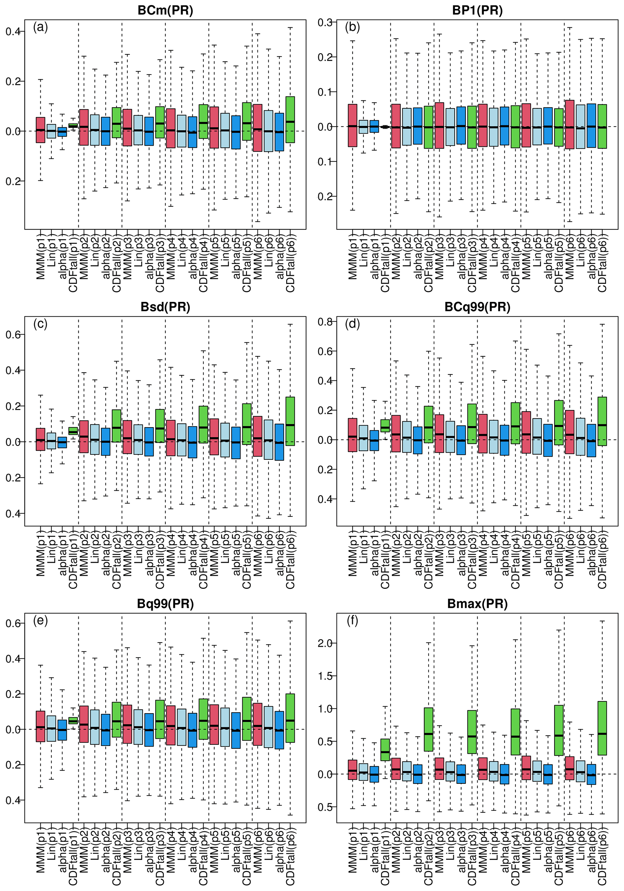
Figure 8 Results of the perfect model experiment for winter precipitation: same as Fig. 7 but for precipitation. The different panels display biases in (a) conditional mean precipitation given a wet state, (b) probability of a dry (< 1 mm) day, (c) standard deviation, (d) conditional 99 % quantile given wet conditions, (e) unconditional 99 % quantile, and (f) maximum precipitation. Results for summer are provided in Fig. S10.

The results from this PME allow us to conclude that the proposed α-pooling method is robust in a climate change context for both temperature and precipitation. In addition, it also indicates that a bias correction technique based on an MMM (i.e. averaging) or linear combination of the GCM CDFs can be useful and robust, although the best results are achieved by the α-pooling technique.

5.3 Sensitivity experiment results

The conclusions brought by the perfect model experiment are based on the pooling and bias correction of five climate models, somewhat arbitrarily selected. One can wonder about the uncertainty or sensitivity of the resulting projected (i.e. future) CDFs of T and PR if other climate models were selected. This is the reason why we perform the sensitivity experiment detailed in Sect. 4.3.

For each of the six selected cities over 2081–2100, Fig. 9 shows the 75 % confidence envelope of the 100 winter temperature CDFs obtained from MMM (red lines), α pooling (blue lines), and linear pooling (light blue lines), as well as the 75 % envelope from the 12 CDF-t results (green lines). Figure 10 show the 75 % confidence envelopes for winter precipitation CDFs. Summer CDF results are given in Figs. S11 and S12 in the Supplement.

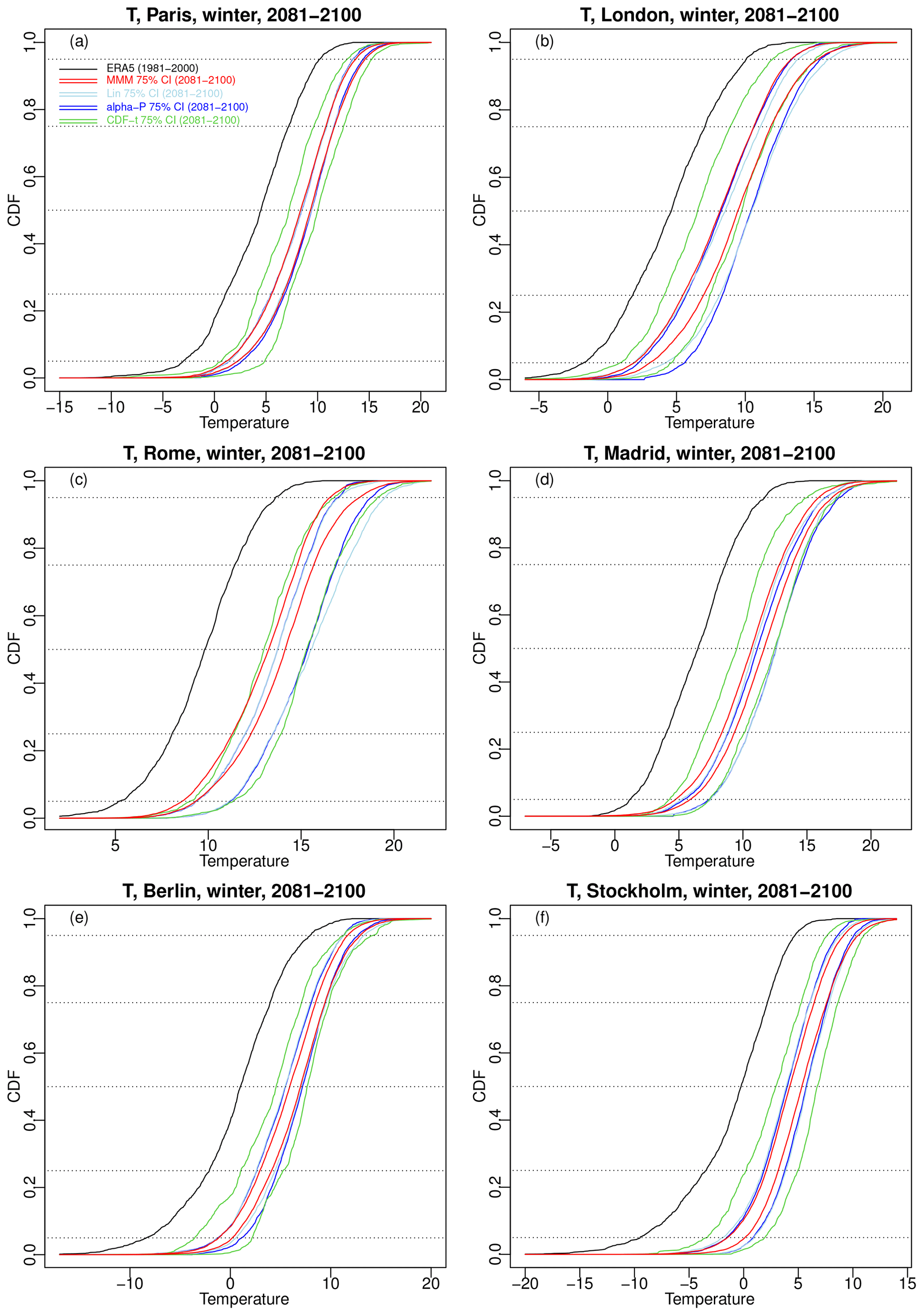
Figure 9 Results of the sensitivity experiment: for winter temperature over 2081–2100 and six major cities in western Europe, 75 % confidence intervals for α pooling (blue lines), linear pooling (light blue lines), MMM (red lines), and CDFt (green lines). The temperature ERA5 CDF (black line) over 1981–2000 is also displayed for visual evaluation of changes. Results for summer are provided in Fig. S11.

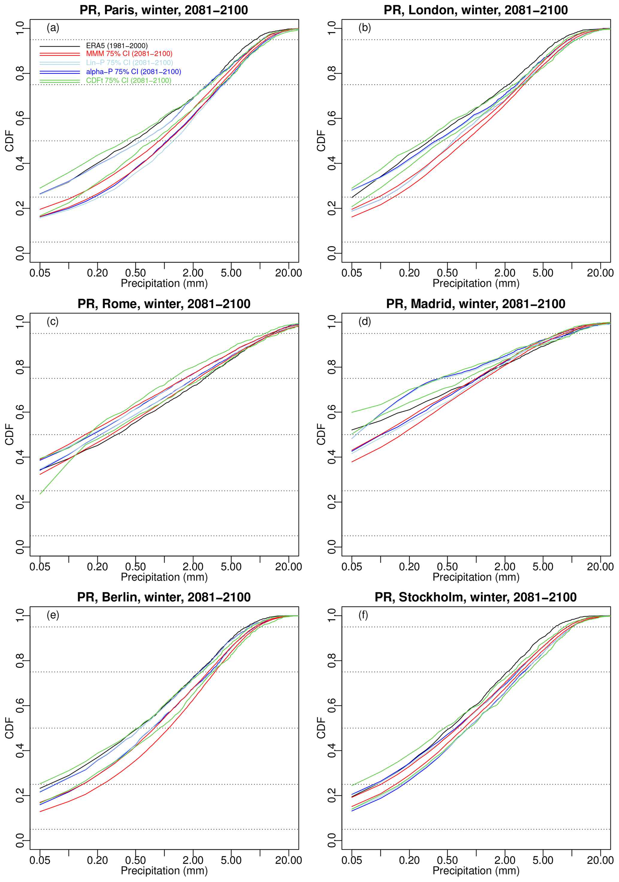
Figure 10 Results of the sensitivity experiment: same as Fig. 9 but for precipitation. Note that the x axis is displayed in log scale to ease evaluation. Results for summer are provided in Fig. S12.

All temperature corrections show a shift of the CDFs towards higher values for all six cities. All combination approaches (i.e. MMM, linear, and α pooling) have very similar 75 % envelopes for Paris (Fig. 9a) and are relatively close for Berlin (Fig. 9e) and Stockholm (Fig. 9f). The other cities present some more differences. The three combination-based methods show similar lower bounds for London but with a higher upper bound for the linear pooling and α-pooling techniques (depending on the quantiles). Rome and Madrid have an MMM envelope shifted towards lower temperature with respect to the other methods. CDF-t 75 % envelopes are generally larger and thus comprise most of the envelopes for any of the six cities. For precipitation (Fig. 10), as expected, the future projections – and thus their corrections – show varying trends depending on the cities. The combination-based methods give 75 % CDF envelopes showing more rain in Paris, London, Berlin, and, to some extent, Stockholm (Fig. 10a, b, e, and f), while they result in less rain in Rome (Fig. 10c). Madrid (Fig. 10d) appears to be the most uncertain for linear and α pooling – whose CDF envelope contains the ERA5 precipitation CDF – while MMM shows more frequent low to medium rain but less frequent heavy rain. For most cities, CDF-t envelopes tend to have lower bounds showing a potential negative shift of the precipitation CDFs with respect to ERA5.

In addition to the position of these envelopes, their size is also important. Hence, the widths of the 75 % CDF confidence envelopes for the six cities over 2081–2100 in winter are given in Fig. 11 for temperature and Fig. 12 for precipitation. For temperature, it is clear that CDF-t has, by far, the largest envelopes widths, while MMM generally has the smallest ones. It was somewhat expected that linear pooling and α pooling would have larger uncertainty than MMM. Indeed, the use of weights means that models with higher weights will have a stronger influence on the resulting CDFs and bias corrections. Thus, even if these models do not closely align with reality during the projection period, their influence can lead to combined projections that can significantly deviate from the simple average performed by MMM. However, there is no such a systematic conclusion for precipitation, showing much more variable rankings, depending on the cities and on the probability values.

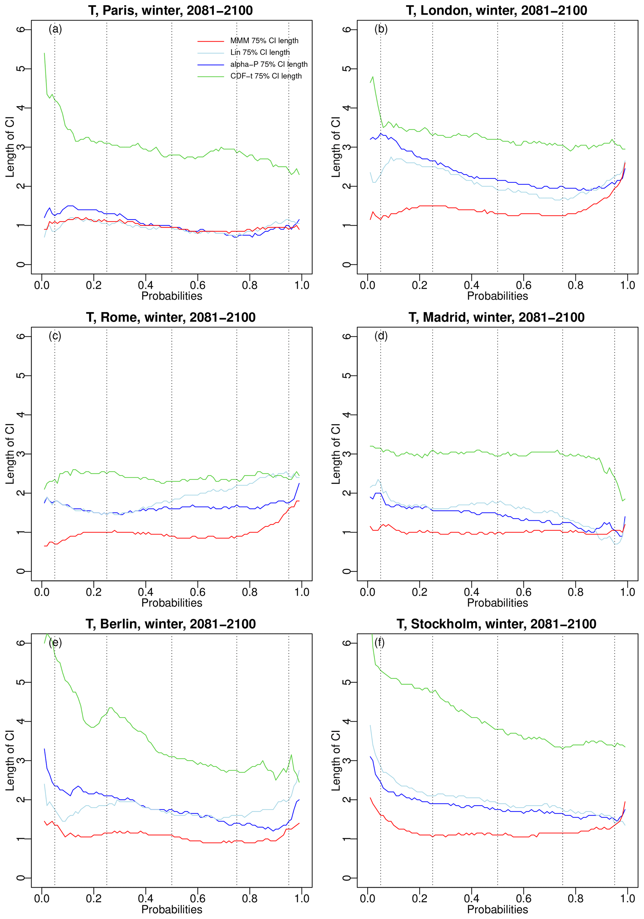
Figure 11 For winter temperature over 2081–2100 and six major cities in western Europe, width of the 75 % CDF confidence intervals for MMM (red line), linear pooling (light blue line), α pooling (blue line), and CDFt (green line). Results for summer are provided in Fig. S13 in the Supplement.

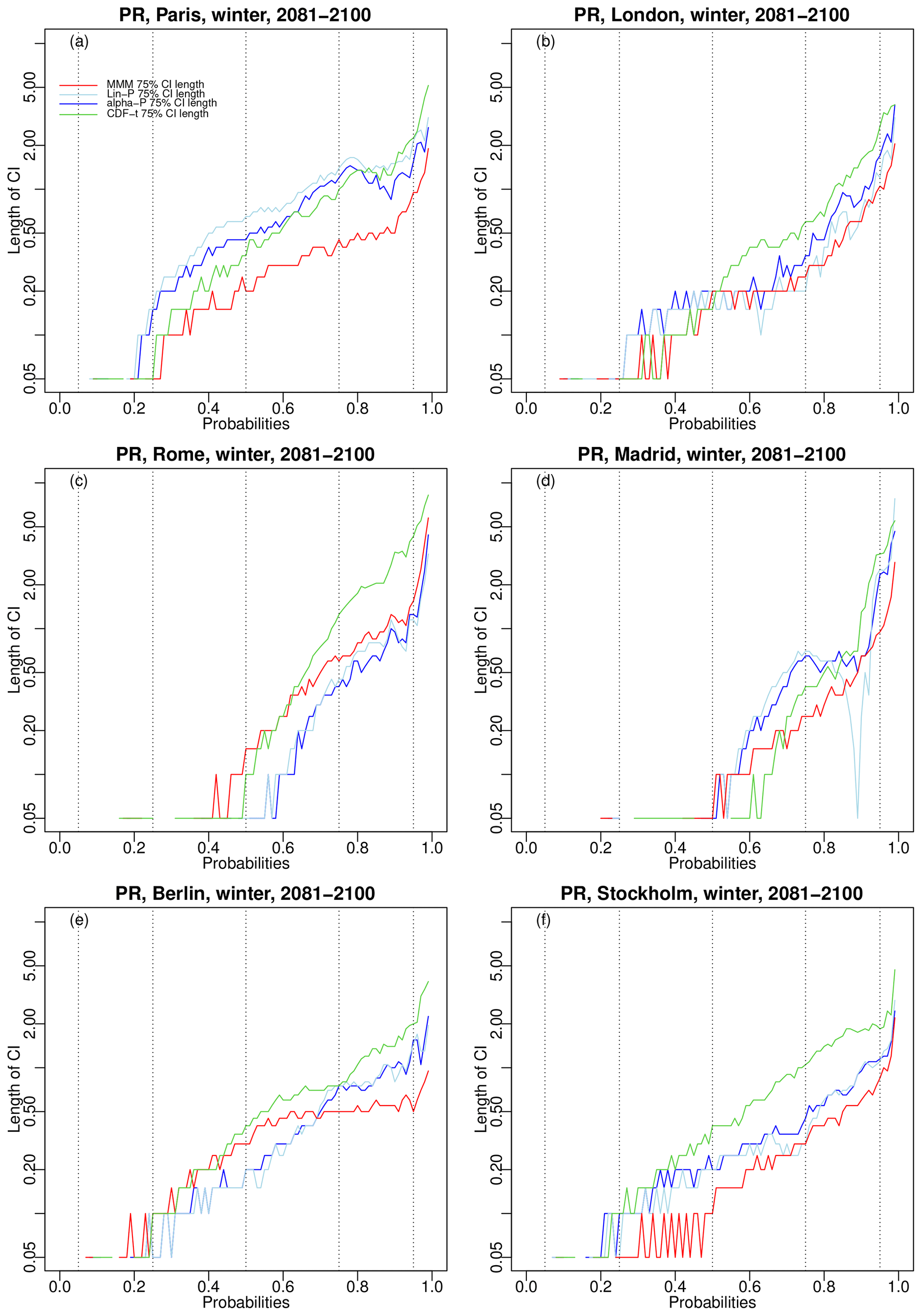
Figure 12 Same as Fig. 11 but for precipitation. Note that the y axis is displayed in log scale to ease evaluation. Results for summer are provided in Fig. S14 in the Supplement.

Globally, the combination-based bias correction methods (MMM, linear, and α pooling) show some robustness in their application to future projections, with uncertainties and sensitivities to the chosen models not being much different from those of the more usual CDF-t technique for precipitation and being even smaller for temperature.

6 Conclusions and perspectives

In this study, we propose a new approach to perform bias correction of climate simulations, taking advantage of combinations of climate models. Combinations are realized via mathematical pooling of cumulative distribution functions (CDFs) – characterizing the variable of interest as simulated by the climate models – to provide a new CDF designed to be more realistic, i.e. closer to a reference CDF over the calibration period. It is important to emphasize that the proposed approach differs from the averaging of quantiles for a given probability as in Markiewicz et al. (2020). It also differs from the usual probability density aggregation, also sometimes called probability fusion (Koliander et al., 2022). Indeed, in our approach, we aggregate cumulative probability distributions. Moreover, our aggregation is indirect in that we aggregate transformed scores instead of directly aggregating the probabilities. In the latter case, we would be restricted to weights summing to 1, whereas in our approach there is no such restriction.

Three pooling strategies have been tested: a CDF multi-model mean (MMM), a linear pooling, and a new approach named α pooling that allows more flexibility, as well as a more traditional bias correction method (CDF-t) applied separately model by model. These four methods have been compared with three different experiments relying on (i) an evaluation with respect to ERA5 reanalyses over a historical period, (ii) a perfect model experiment (PME) over future time periods, and (iii) a sensitivity analysis to the choice of the climate models to combine.

In a cross-validation framework over the historical period (experiment (i), Sect. 5.1), the four methods generally behave similarly, with most biases relatively well centred around 0 in both temperature and precipitation. However, the application of the “pure” bias correction method CDF-t to separate GCMs can generate more biases with more variability. This is because the change (in temperature or precipitation) simulated by a single climate model over the historical period may not correspond to the change present in the reanalyses. By combining CDFs coming from different GCMs, the pooling techniques also combine the evolution (i.e. changes) over time, resulting in bias-corrected projections that are more consistent with the reanalyses.

The results of the PME show a good robustness of the three pooling strategies, even for the MMM approach, with biases of most statistics (including extremes) around 0. Moreover, the biases in high quantiles, especially for maximum values, are much lower for pooling-based methods than for traditional BC methods represented here by CDF-t. Overall, a quasi-systematic ranking of the four methods is observed in this PME: while CDF-t can present some recurrent and pronounced biases – getting larger for further time periods – the MMM correction approach improves the results; the linear approach improves the results even more, and the best results are obtained with the α-pooling technique for both variables. This confirms the benefits of combining the information (here CDFs) from different models to perform bias correction, even in a strong climate change context. This is in agreement with results from Vrac et al. (2022), who showed, in a slightly different context, that accounting for the evolution of the mean temperature–precipitation correlation in an ensemble of climate models allows getting more robust estimates of future dependencies.

However, the CDFs resulting from our linear or α-pooling approaches might depend on the selected ensemble of model CDFs to combine. Hence, the choice of the models to combine remains key as it necessarily influences the results over the (future) projection periods. Note, nevertheless, that this is true for any combination strategy – i.e. not only our proposed pooling methods – or for any bias correction technique where the choice of the model simulation to correct will also necessarily affect the final results (e.g. time series, CDFs). We also note here that for the combination methods that include weights (i.e. linear and α pooling), the numerical optimization of the weights results in redundant CDFs receiving low weights. For instance, if two models result in the exact same CDF, the optimization will result in weights that will be shared between these identical CDFs and whose total would be the weight corresponding to this CDF not being duplicated. This is an important feature as it is known that some models are closely related and, thus, tend to provide similar forecasts.

The sensitivity analysis of the future (2081–2100) CDFs to the choice of the ensemble of models shows that the uncertainty in long-term projections was found to be globally comparable for the three pooling-based methods, although it is slightly higher for α pooling and slightly lower for MMM pooling. Indeed, as the α pooling and linear pooling associate non-uniform weights with the different CDFs, they pull the results towards the models with the highest weights, hence generating more variability depending on the selected ensemble of models to combine. Conversely, the MMM pooling corresponds to a linear pooling with weights forced to be uniform. Therefore, it provides smoother CDF results that are less sensitive to the choice of the ensemble. The opposite example is given by CDF-t that is applied model by model and thus shows a high sensitivity to the selected ensemble. While MMM pooling has the potential to lead to overly confident projections, our novel pooling method may offer a more realistic representation of scenario uncertainty. Nevertheless, it is crucial to acknowledge the potential for our α-pooling method to introduce unrealistic scenario uncertainty. This aspect warrants further investigation in future studies, especially for practical applications.

In terms of computation time, it is obvious that alpha pooling is more computationally demanding than linear or MMM pooling. This is in part due to the additional parameter α but mostly to the non-linearity induced by α pooling. However, for the combination of up to 10 climate models (i.e. CDFs), the computational time for each location and variable time series typically does not exceed a few minutes. Given the substantial computational demands associated with running individual climate models, the computational aspect of combining them is trivial by comparison. Moreover, considering that this post-processing of climate simulations does not need to be performed on a daily basis but rather once for all, we believe that this represents a reasonable computational cost, ensuring the method's practical applicability without compromise.

As a conclusion, the α-pooling model appears to be a promising approach for pooling model CDFs. More generally, the results of this study show that the CDF pooling strategy for “multi-model bias correction” is a credible alternative to usual GCM-by-GCM correction methods by allowing handling and considering several climate models at once.

This work can be extended in various ways. First, even though only temperature and precipitation were considered in this study, many other climate variables – such as wind and humidity – can be handled with this CDF pooling strategy. Also, the proposed pooling method can be directly applied to regional climate model simulations, instead of GCM simulations, in order to get more regional views of climate changes.

In addition, some more technical and statistical developments could be made to improve the CDF pooling approach. For example, the present linear pooling and α-pooling methods are based on the L² norm to estimate the parameters. Other distances could be used, more specifically distances between distribution functions, e.g. the Hellinger distance, the total variation distance (Clarotto et al., 2022), the Wasserstein distance (e.g., Santambrogio, 2015; Robin et al., 2019), or the Kullback–Leibler divergence (Kullback and Leibler, 1951). Such distribution-based distances could potentially improve the quality of the fit and then provide more robust pooled CDFs.

Moreover, even though spatial patterns are visible in the parameters, there is variability between nearby grid cells that complicates the interpretation of the parameters (see Figs. 3 and 4). Such variability can be reduced by constraining the approach to provide more continuous and smoother spatial structures, presumably at the cost of longer computations.

Also note that it would be interesting to account for rainfall specificities when applying a CDF pooling strategy to precipitation. Indeed, in this study, the pooling was applied to all daily precipitation values. In practice, a distinction between dry day frequencies and distributions of wet intensity could be made by having two separate poolings. Although the α-pooling results for precipitation in this article were quite satisfying, such a rainfall-specific design could provide additional improvements and should be tested in the future.

Other modelling extensions could be considered. One interesting aspect could be to focus on extreme events. For example, α pooling could be applied to conditional CDFs above a high threshold related to the tail of the whole distribution or applied to the CDF of block maxima. Distributions stemming from the extreme value theory – such as the generalized Pareto distribution (GPD) or the generalized extreme value distribution (GEV) – would then have to be used. Besides the practical results that such an application could bring, the statistical properties of the resulting pooled (extreme) CDFs would also be worth studying from a theoretical point of view.

Another interesting perspective, in terms of both practical and theoretical aspects, concerns the extension of the α pooling to the multivariate context. Indeed, so far, this pooling method has been developed and applied only in a univariate framework; i.e. different variables (temperature and precipitation) are handled, combined, and bias-corrected separately. An extension of α pooling allowing the combination of joint (i.e. multivariate) CDFs would allow improving the modelling of dependencies between the variables and, thus, providing more realistic inter-variable CDFs and bias-corrected projections. Such an extended α pooling should then be compared to other multivariate bias correction methods, such as those studied in François et al. (2020). It would then also allow investigating compound events (e.g. Zscheischler et al., 2018, 2020) and their potential future changes more robustly.

Finally, more generally, it is worth noting that combination and bias correction are not new questions or requirements. However, this is the first paper coupling methods from these two domains. This was made possible by our pooling strategy working on CDFs (and not on specific quantiles or statistical properties such as mean and max, as usually done), which is, in itself, an original contribution to the combination framework. This CDF pooling strategy and this hybrid combination–correction method deserve to be further explored, as do its potential applications beyond combination and bias correction.

Appendix A: An approximate solution to the α pooling

The well-known Box–Cox transformation $B\left(F\right)\left(x\right)=(\mathrm{1}-F(x{)}^{\mathit{\alpha }})/\mathit{\alpha }$, with α>0, is well defined for all values $F\left(x\right)\in [\mathrm{0},\mathrm{1}]$, with ${lim}_{\mathit{\alpha }\to \mathrm{0}}B\left(F\right)\left(x\right)=-\ln F\left(x\right)$ when F(x)>0 and ${lim}_{\mathit{\alpha }\to \mathrm{0}}B(\mathrm{1}-F)\left(x\right)=-\ln (\mathrm{1}-F(x\left)\right)$ when F(x)<1. Let us consider a pooling approach that consists of assuming that the Box–Cox transformation of the pooled CDF is, up to a normalizing factor K, the weighted average of the Box–Cox transformation, i.e.

$${\displaystyle }\begin{array}{rl}{\displaystyle }& {\displaystyle }B(K.F_B)\left(x\right)={\sum }_{i=\mathrm{1}}^N{w}_{i}B\left(F_i\right)\left(x\right)\mathrm{\text{and}}\\ {\displaystyle }& {\displaystyle }B(K.(\mathrm{1}-F_B\left)\right)\left(x\right)={\sum }_{i=\mathrm{1}}^N{w}_{i}B(\mathrm{1}-F_i)\left(x\right).\end{array}$$

After multiplying by α and rearranging, one gets

$${\displaystyle }\begin{array}{rl}{\displaystyle }& {\displaystyle }{K}^{\mathit{\alpha }}{F}_B(x{)}^{\mathit{\alpha }}=\mathrm{1}+{\sum }_{i=\mathrm{1}}^N{w}_i(F_i(x{)}^{\mathit{\alpha }}-\mathrm{1})\mathrm{\text{and}}\\ {\displaystyle }& {\displaystyle }{K}^{\mathit{\alpha }}(\mathrm{1}-F_B(x){)}^{\mathit{\alpha }}=\mathrm{1}+{\sum }_{i=\mathrm{1}}^N{w}_i(\mathrm{1}-F_i\left(x\right){)}^{\mathit{\alpha }}-\mathrm{1}).\end{array}$$

From the fact that $F_B\left(x\right)+\mathrm{1}-F_B\left(x\right)=\mathrm{1}$, one thus gets

$$\begin{array}{}\text{(A1)}& {\displaystyle }\begin{array}{rl}{\displaystyle }& {\displaystyle }{F}_B\left(x\right)=\\ {\displaystyle }& {\displaystyle \frac{[\mathrm{1}-S+{\sum }_{i=\mathrm{1}}^N{w}_i{F}_i(x{)}^{\mathit{\alpha }}{]}^{\mathrm{1}/\mathit{\alpha }}}{\left\{\begin{array}{c}[\mathrm{1}-S+{\sum }_{i=\mathrm{1}}^N{w}_i{F}_i(x{)}^{\mathit{\alpha }}{]}^{\mathrm{1}/\mathit{\alpha }}+\\ [\mathrm{1}-S+{\sum }_{i=\mathrm{1}}^N{w}_i(\mathrm{1}-F_i\left(x\right){)}^{\mathit{\alpha }}{]}^{\mathrm{1}/\mathit{\alpha }}\end{array}\right\}}},\forall x\in \mathbb{R},\end{array}\end{array}$$

with $S={\sum }_{i=\mathrm{1}}^N{w}_i$.

Let us now go back to the α-pooling approach described in Sect. 3.4. Inspired by Eq. (A1), let us plug into the α pooling in Eq. (7) a solution of the form $F_H(x{)}^{\mathit{\alpha }}=({\sum }_{i=\mathrm{1}}^N{w}_i{F}_i(x{)}^{\mathit{\alpha }}+A)/Z$ and $(\mathrm{1}-F_H(x){)}^{\mathit{\alpha }}=({\sum }_{i=\mathrm{1}}^N{w}_i(\mathrm{1}-F_i(x){)}^{\mathit{\alpha }}+A)/Z$, where Z is a normalizing factor. From $F_H\left(x\right)+\mathrm{1}-F_H\left(x\right)=\mathrm{1}$ we find that $Z^{\mathrm{1}/\mathit{\alpha }}=\left[{\sum }_{i=\mathrm{1}}^N{w}_i{F}_i\right(x{)}^{\mathit{\alpha }}+A{]}^{\mathrm{1}/\mathit{\alpha }}+\left[{\sum }_{i=\mathrm{1}}^N{w}_i\right(\mathrm{1}-F_i\left(x\right){)}^{\mathit{\alpha }}+A{]}^{\mathrm{1}/\mathit{\alpha }}$ and

$${\displaystyle }{F}_H\left(x\right)={\displaystyle \frac{\left[{\sum }_{i=\mathrm{1}}^N{w}_i{F}_i\right(x{)}^{\mathit{\alpha }}+A{]}^{\mathrm{1}/\mathit{\alpha }}}{\left\{\begin{array}{c}\left[{\sum }_{i=\mathrm{1}}^N{w}_i{F}_i\right(x{)}^{\mathit{\alpha }}+A{]}^{\mathrm{1}/\mathit{\alpha }}+\\ \left[{\sum }_{i=\mathrm{1}}^N{w}_i\right(\mathrm{1}-F_i\left(x\right){)}^{\mathit{\alpha }}+A{]}^{\mathrm{1}/\mathit{\alpha }}\end{array}\right\}}},$$

which is nothing but Eq. (A1) with $A=\mathrm{1}-S$. Hence F_H=F_B, and for the rest of this section, we will use the notation F_B for both constructions. F_B is well defined for all α>0 if S≤1. In this case, it can be shown that it is a non-decreasing function of x because its derivative with respect to x is non-negative. From

$$\begin{array}{}\text{(A2)}& {\displaystyle }\begin{array}{rl}{\displaystyle }& {\displaystyle }\underset{x\to -\mathrm{\infty }}{lim}{F}_B\left(x\right)={\displaystyle \frac{(\mathrm{1}-S{)}^{\mathrm{1}/\mathit{\alpha }}}{(\mathrm{1}-S{)}^{\mathrm{1}/\mathit{\alpha }}+\mathrm{1}}}\mathrm{\text{and}}\\ {\displaystyle }& {\displaystyle }\underset{x\to \mathrm{\infty }}{lim}{F}_B\left(x\right)={\displaystyle \frac{\mathrm{1}}{(\mathrm{1}-S{)}^{\mathrm{1}/\mathit{\alpha }}+\mathrm{1}}},\end{array}\end{array}$$

one finds that F_B in Eq. (A1) is a proper CDF if and only if the condition S=1 is verified. In this case, F_B has the simpler expression

$$\begin{array}{}\text{(A3)}& {\displaystyle }{F}_{B,\mathrm{1}}\left(x\right)={\displaystyle \frac{\left[{\sum }_{i=\mathrm{1}}^N{w}_i{F}_i\right(x{)}^{\mathit{\alpha }}{]}^{\mathrm{1}/\mathit{\alpha }}}{\left\{\begin{array}{c}\left[{\sum }_{i=\mathrm{1}}^N{w}_i{F}_i\right(x{)}^{\mathit{\alpha }}{]}^{\mathrm{1}/\mathit{\alpha }}+\\ \left[{\sum }_{i=\mathrm{1}}^N{w}_i\right(\mathrm{1}-F_i\left(x\right){)}^{\mathit{\alpha }}{]}^{\mathrm{1}/\mathit{\alpha }}\end{array}\right\}}}.\end{array}$$

When α=1, the pooling formula (Eq. A3) reduces to the linear pooling. As α→0, it is straightforward to check that it boils down to the log-linear pooling (Eq. 4). As was the case for the α pooling presented in Sect. 3.4, this pooling formula thus generalizes both the log-linear pooling and the linear pooling. It must be emphasized that replacing w_i by Kw_i with K>0 in Eq. (A3) leads to the same value F_B,1(x). Imposing ${\sum }_{i=\mathrm{1}}^N{w}_i=\mathrm{1}$ or not in Eq. (A3) thus has no consequences for F_B,1.

The existence of two different pooling approaches, namely F_G and F_B, calls for some comments.

• In numerous tests, it was consistently found that the CDF F_G obtained by the α pooling (Eq. 7) and the CDF F_B,1 computed directly using Eq. (A3) are almost indistinguishable when imposing S=1. In this case, the direct computation in Eq. (A3) is 5 to 10 times faster and should be preferred.

• However, as discussed in Sect. 3.4, F_G is a proper CDF even if S>1. There is thus an extra parameter available for the α-pooling approach, allowing for a better fit between the models and the reference. The cost is increased computation time.

• When using the direct approach in Eq. (A1), S≤1 leads to well-defined values F_B(x). It thus also offers an extra parameter for the pooling, but the CDF F_B varies between the limits in Eq. (A2) instead of [0,1]. Strictly speaking, F_B is thus not a proper CDF. In practice, however, it was very often found that the quantity $\left(\right(\mathrm{1}-S{)}^{\mathrm{1}/\mathit{\alpha }}+\mathrm{1}{)}^{-\mathrm{1}}$ was extremely small (say, less than 10⁻³) and the min–max rescaling shown in Eq. (11) can be performed to get a proper CDF.

• In Eq. (A1) S>1 must be avoided as it can lead to inconsistent results, such as non monotonic functions F_B.

Appendix B: Optimal properties of α pooling

We briefly report some optimal properties of the α pooling presented in Sect. 3.4. We refer to Neyman and Roughgarden (2023) for a complete presentation on proper scoring rules, quasi-arithmetic pooling, and min–max optimal properties. We first start with some generalities. For the sake of clarity, x is fixed and we write F for F(x). We further define the vector $\mathit{F}=(F,\mathrm{1}-F{)}^t$. In what follows, vectors will be written in bold letters.

The accuracy of a pooling method for a probability distribution is assessed using a metric, called a scoring rule, which assigns a value (sometimes called a reward) when a probability q is reported and outcome j happens according to a reference probability p. Among all possible scoring rules, we will restrict ourselves to proper scoring rules, i.e. a scoring rule that is maximized when the reported probability is q=p. Well-known examples of proper scoring rules are the Brier scoring rule (Brier et al., 1950) and the logarithmic scoring rule. As shown in Gneiting and Raftery (2007) and in Neyman and Roughgarden (2023, Theorem 3.1), proper scoring rules can be derived from a function G(p), referred to as the expected reward function. According to this theorem a scoring rule is proper if and only if

$$\begin{array}{}\text{(B1)}& s(\mathit{p};j)=G\left(\mathit{p}\right)+\langle \mathit{g}\left(\mathit{p}\right),{\mathit{\delta }}_j-\mathit{p}\rangle ,\end{array}$$

where g(p) is the gradient of G(p). Let $j=\mathrm{1},\mathrm{\dots },J$ be the possible outcomes with probabilities $\mathit{p}=\left(p\right(\mathrm{1}),\mathrm{\dots },p(J\left)\right)$. The Brier (also known as “quadratic”) scoring rule corresponds to $G_{\text{Brier}}\left(\mathit{p}\right)={\sum }_{j}p(j{)}^{\mathrm{2}}$ and the logarithmic scoring rule corresponds to $G_{\text{log}}\left(\mathit{p}\right)={\sum }_{j}p\left(j\right)\ln p\left(j\right)$. A necessary condition on G is that it is a convex function with respect to p. Neyman and Roughgarden (2023) call quasi-arithmetic pooling any pooling formula defined by

$$\begin{array}{}\text{(B2)}& {\displaystyle }\begin{array}{rl}{\displaystyle }\mathit{g}\left({\mathit{F}}_G\right)& {\displaystyle }={\sum }_{i=\mathrm{1}}^N{w}_i\mathit{g}\left({\mathit{F}}_i\right),\\ {\displaystyle }& {\displaystyle }{w}_i\ge \mathrm{0},i=\mathrm{1},\mathrm{\dots },N,{\sum }_{i=\mathrm{1}}^N{w}_i=\mathrm{1},\end{array}\end{array}$$

where g is the gradient of a proper scoring rule G. They show (in Theorem 4.1) the following max–min property for quasi-arithmetic pooling formula. Let us define the following utility function,

$$\begin{array}{}\text{(B3)}& u(\mathit{F};j):=s(\mathit{F};j)-\sum _{i=\mathrm{1}}^N{w}_{i}s({\mathit{F}}_i;j)\end{array}$$

which corresponds to the expected difference between the scoring rule applied to F and the scoring rule applied to model i, chosen randomly according to w. Then, the minimum ${min}_{F}u(\mathit{F};j)$ is maximized by setting F=F_G as given in Eq. (B2). In other words, the worst loss of scores (often interpreted as a reward) is maximized using quasi-arithmetic pooling.

In our case, for a given x, there are only two possible outcomes, $j\in \mathit{\{}\mathrm{0},\mathrm{1}\mathit{\}}$: being less than or equal to x, with probability p(0)=F, and being above s, with probability $p\left(\mathrm{1}\right)=\mathrm{1}-F$. We now consider the following convex function:

$$\begin{array}{}\text{(B4)}& G\left(\mathit{F}\right)=F^{\mathrm{1}+\mathit{\alpha }}+(\mathrm{1}-F{)}^{\mathrm{1}+\mathit{\alpha }},\end{array}$$

with the limit case ${lim}_{\mathit{\alpha }\to \mathrm{0}}G\left(\mathit{F}\right)=F\ln F+(\mathrm{1}-F)\ln (\mathrm{1}-F)$ corresponding to the logarithmic scoring rule. Notice that α=1 corresponds to the Brier scoring rule. The associated gradient is

$$\begin{array}{}\text{(B5)}& \mathit{g}\left(\mathit{F}\right)=(\mathrm{1}+\mathit{\alpha })(F^{\mathit{\alpha }},(\mathrm{1}-F{)}^{\mathit{\alpha }}{)}^t,\end{array}$$

with ${lim}_{\mathit{\alpha }\to \mathrm{0}}\mathit{g}\left(\mathit{F}\right)=(\mathrm{1}+\ln F,\mathrm{1}+\ln (\mathrm{1}-F){)}^t$. Since in Eq. (B4) the function G is convex, the scoring rule given by Eq. (B1) is proper and each component of the gradient is a continuous and injective function of F for all values α≥0. The scoring rule associated with G(F) in Eq. (B4) thus varies continuously from the logarithmic scoring rule to the Brier scoring rule as α varies from 0 to 1. Notice that α is also allowed to be larger than 1, but the scoring rule has no specific name in that case. The pooling formula defined by

$$\begin{array}{}\text{(B6)}& {\displaystyle }\begin{array}{rl}{\displaystyle }{\mathit{H}}_{\mathrm{2}}\mathit{g}\left({\mathit{F}}_G\right)& {\displaystyle }={\sum }_{i=\mathrm{1}}^N{w}_i{\mathit{H}}_{\mathrm{2}}\mathit{g}\left({\mathit{F}}_i\right),\\ {\displaystyle }& {\displaystyle }{w}_i\ge \mathrm{0},i=\mathrm{1},\mathrm{\dots },N,{\sum }_{i=\mathrm{1}}^N{w}_i=\mathrm{1},\end{array}\end{array}$$

where H₂ is the (1,2) Helmert matrix, corresponds exactly to the α pooling presented in Sect. 3.4, which thus inherits the optimal properties of quasi-arithmetic pooling.